$T$-optimal designs for discrimination between two polynomial models

Abstract

This paper is devoted to the explicit construction of optimal designs for discrimination between two polynomial regression models of degree $n-2$ and $n$. In a fundamental paper, Atkinson and Fedorov [Biometrika 62 (1975a) 57–70] proposed the $T$-optimality criterion for this purpose. Recently, Atkinson [MODA 9, Advances in Model-Oriented Design and Analysis (2010) 9–16] determined $T$-optimal designs for polynomials up to degree 6 numerically and based on these results he conjectured that the support points of the optimal design are cosines of the angles that divide half of the circle into equal parts if the coefficient of $x^{n-1}$ in the polynomial of larger degree vanishes. In the present paper we give a strong justification of the conjecture and determine all $T$-optimal designs explicitly for any degree $n\in\mathbb{N}$. In particular, we show that there exists a one-dimensional class of $T$-optimal designs. Moreover, we also present a generalization to the case when the ratio between the coefficients of $x^{n-1}$ and $x^{n}$ is smaller than a certain critical value. Because of the complexity of the optimization problem, $T$-optimal designs have only been determined numerically so far, and this paper provides the first explicit solution of the $T$-optimal design problem since its introduction by Atkinson and Fedorov [Biometrika 62 (1975a) 57–70]. Finally, for the remaining cases (where the ratio of coefficients is larger than the critical value), we propose a numerical procedure to calculate the $T$-optimal designs. The results are also illustrated in an example.

T1Supported in part by the Collaborative Research Center “Statistical modeling of nonlinear dynamic processes” (SFB 823, Teilprojekt C2) of the German Research Foundation (DFG).

, and

t2Supported in part by Russian Foundation of Basic Research (Project 09-01-00508).

1 Introduction

The problem of identifying an appropriate model in a class of competing regression models is of fundamental importance in regression analysis, and it occurs often in real experimental studies. It is widely accepted nowadays that good experimental designs can improve the performance of discrimination, and several authors have addressed the problem of constructing optimal designs for this purpose; see Hunter and Reiner (1965), Stigler (1971), Atkinson and Fedorov (1975a, 1975b), Hill (1978), Fedorov (1980), Denisov, Fedorov and Khabarov (1981), Studden (1982), Fedorov and Khabarov (1986), Spruill (1990), Dette (1994, 1995), Dette and Haller (1998), Song and Wong (1999), Uciński and Bogacka (2005), Wiens (2009, 2010) among many others. In a fundamental paper, Atkinson and Fedorov (1975a) introduced the $T$-optimality criterion for discriminating between two competing regression models. As an example, these authors constructed $T$-optimal designs for a constant and a quadratic model. Since its introduction, the problem of determining $T$-optimal designs has been considered by numerous authors; see Atkinson and Fedorov (1975b), Uciński and Bogacka (2005), Wiens (2009), Tommasi and López-Fidalgo (2010), among others. In order to demonstrate the benefits of the $T$-optimal design, we display, in Table 1, the simulated power of the $F$-test for the hypothesis $H_{0}\dvtx\theta_{2,2}=\theta_{2,3}=0$ in the cubic regression model $\eta(x,\theta)=\sum^{3}_{j=0}\theta_{2j}x^{j}$ on the interval $[-1,1]$ (with standard normal distributed errors), where observations are taken according to two designs. The first design is the commonly used equidistant design with $12$ observations at the four points, $-1,-1/3,1/3$ and $1$, respectively, while the second design is a $T$-optimal design, as considered in this paper, with $8$ observations at the two points, $-1,1$ and $16$ observations at the two points $-1/2,1/2$, respectively. We observe clear advantages (with respect to the power of the $F$-test) for the $T$-optimal design.

=270pt $\bolds{\theta_{2,3}}$ $\bolds{0}$ $\bolds{0.5}$ $\bolds{1.0}$ $\bolds{1.5}$ $\bolds{2.0}$ $T$-optimal $0.051$ $0.104$ $0.301$ $0.641$ $0.896$ Equidistant $0.053$ $0.092$ $0.218$ $0.438$ $0.638$

Table 1: Simulated power of the $F$-test in a cubic regression model $\sum^{3}_{j=0}\theta_{2j}x^{j}$ for the hypothesis of linear regression model for various values of $\theta_{2,3}$ and different designs $(\theta_{2,2}=0)$

Since its introduction $T$-optimal designs have found numerous applications including such important fields as chemistry of pharmacokinetics; see Atkinson, Bogacka and Bogacki (1998), Asprey and Macchietto (2000), Uciński and Bogacka (2005) or Foo and Duffull (2011) among others. The $T$-optimal design problem is essentially a minimax problem, and, except for very simple models, the corresponding optimal designs are not easy to find and have to be determined numerically. In a recent paper, Dette and Titoff (2009) discussed the $T$-optimal design problem from a general point of view and related it to a nonlinear problem in approximation theory. As an illustration, designs for discriminating between a linear model and a cubic model without quadratic term were presented, and it was shown that $T$-optimal designs are, in general, not unique.

Atkinson (2010) considered a similar problem of this type and studied the problem of discriminating between two competing polynomial regression models which differ in the degree by two. This author determined $T$-optimal designs for polynomials up to degree $6$ numerically where the coefficient of $x^{n-1}$ in the polynomial of larger degree (say $n$) vanishes. Based on these results he conjectured that the support points of the $T$-optimal design are cosines of angles dividing a half of circle into equal parts.

The present paper has two purposes. In particular, we prove the conjecture raised in Atkinson (2010) and derive explicit solutions of the $T$-optimal design problem for discriminating between polynomial regression models of degree $n-2$ and $n$ for any $n\in\mathbb{N}$. Moreover, we also determine the $T$-optimal designs analytically in the case when the ratio of the coefficients of the terms $x^{n-1}$ and $x^{n}$ is sufficiently small. The situation considered in Atkinson (2010) corresponds to the case where this ratio vanishes, and in this case we show that there exists a one-dimensional class of $T$-optimal designs. To the best of our knowledge these results provide the first explicit solution of the $T$-optimal design problem in a nontrivial situation. Our results provide further insight into the complicated structure of the $T$-optimal design problem. Finally, in the case where the coefficient exceeds the critical value, we suggest a procedure to determine the $T$-optimal design numerically.

2 The $T$-optimal design problem revisited

Consider the classical regression model

$$y=\eta(x)+\varepsilon,$$ (1)

where the explanatory variable $x$ varies in the design space $\cal X$, and observations at different locations, say $x$ and $x^{\prime}$, are assumed to be uncorrelated with the same variance. In (1) the quantity $\varepsilon$ denotes a random variable with mean $0$ and variance $\sigma^{2}$, and $\eta$ is a function, which is called regression function in the literature. We assume that the experimenter has two parametric models for this function in mind, that is,

$$\eta_{1}(x,\theta_{1})\quad\mbox{and}\quad\eta_{2}(x,\theta_{2}),$$ (2)

and the first goal of the experiment is to discriminate between these two models. In (2) the quantities $\theta_{1}$ and $\theta_{2}$ denote unknown parameters which vary in compact parameter spaces, say $\Theta_{1}\subset\mathbb{R}^{m_{1}}$ and $\Theta_{2}\subset\mathbb{R}^{m_{2}}$, and have to be estimated from the data. In order to find “good” designs for discriminating between the models $\eta_{1}$ and $\eta_{2}$, we consider approximate designs in the sense of Kiefer (1974), which are defined as probability measures on the design space $\mathcal{X}$ with finite support. The support points of an (approximate) design $\xi$ give the locations where observations are taken, while the weights give the corresponding relative proportions of total observations to be taken at these points. If the design $\xi$ has masses $\omega_{i}>0$ at the different points $x_{i}$ $(i=1,\ldots,k)$, and $N$ observations can be made by the experimenter, the quantities $\omega_{i}N$ are rounded to integers, say $n_{i}$, satisfying $\sum^{k}_{i=1}n_{i}=N$, and the experimenter takes $n_{i}$ observations at each location $x_{i}$ $(i=1,\ldots,k)$.

To determine a good design for discriminating between the models $\eta_{1}$ and $\eta_{2}$ [Atkinson and Fedorov (1975a)] proposed in a fundamental paper to fix one model, say $\eta_{1}$ (more precisely its corresponding parameter $\theta_{1}$), and to determine the design which maximizes the minimal deviation between the model $\eta_{1}$ and the class of models defined by $\eta_{2}$, that is,

$$\xi^{*}=\mathop{\arg\max}_{\xi}\int_{\chi}\bigl{(}\eta_{1}(x,\theta_{1})-\eta_{2}(x,\theta_{2}^{*})\bigr{)}^{2}\xi(dx),$$

where the parameter ${\theta}_{2}^{*}$ minimizes the expression

$${\theta}_{2}^{*}=\mathop{\arg\min}_{\theta_{2}\in\Theta_{2}}\int_{\chi}\bigl{(}\eta_{1}(x,\theta_{1})-\eta_{2}(x,\theta_{2})\bigr{)}^{2}\xi(dx).$$

Note that $\theta^{*}_{2}$ is not an estimate, but it corresponds to the best approximation of the “given” model $\eta_{1}(\cdot,\theta_{1})$ by models of the form $\{\eta_{2}(\cdot,\theta_{2})\mid\theta_{2}\in\Theta_{2}\}$ with respect to a weighted $L_{2}$-norm. Since its introduction the $T$-optimal design problem has found considerable interest in the literature, and we refer the interested reader to the work of Uciński and Bogacka (2005) or Dette and Titoff (2009), among others. In general, the determination of $T$-optimal designs is a very difficult problem, and explicit solutions are—to our best knowledge—not available except for very simple models with a few parameters. In this paper we present analytical results for $T$-optimal designs, if the interest is in the discrimination between two polynomial models which differ in the degree by two. To be precise, we consider the case where the regression functions $\eta_{1}(x,\theta_{1})$ and $\eta_{2}(x,\theta_{2})$ are given by

$$\quad\eta_{1}(x,\theta_{1})=\theta_{1,0}+\theta_{1,1}x+\cdots+\theta_{1,n-2}x^{n-2}+\theta_{1,n-1}x^{n-1}+\theta_{1,n}x^{n}$$ (3)

and

$$\eta_{2}(x,\theta_{2})=\theta_{2,0}+\theta_{2,1}x+\cdots+\theta_{2,n-2}x^{n-2},$$ (4)

respectively, and the design space is given by $\mathcal{X}=[-1,1]$. In model (3) the parameter $\theta_{1}$ is given by $\theta_{1}=(\theta_{1,0},\theta_{1,1},\ldots,\theta_{1,n-2},b\theta_{1,n},\theta_{1,n})^{T}$, where the ratio of the coefficients corresponding to the highest powers $b=\theta_{1,n-1}/\theta_{1,n}$ and the parameter $\theta_{1,n}$ specify the deviation from a polynomial of degree $n-2$.

In the following discussion, we define

$$\bar{\eta}(x,\alpha,b,\theta_{1,n}) = \eta_{1}(x,\theta_{1})-\eta_{2}(x,\theta_{2})$$

$$= \alpha_{0}+\alpha_{1}x+\cdots+\alpha_{n-2}x^{n-2}+\theta_{1,n}(bx^{n-1}+x^{n}),$$

where we use the notation $\alpha_{i}=\theta_{1,i}-\theta_{2,i}$ $(i=0,\ldots,n-2)$; then the problem of finding the $T$-optimal design for the models $\eta_{1}$ and $\eta_{2}$ can be reduced to

$$\xi^{*}=\mathop{\arg\max}_{\xi}\int_{\chi}\bigl{(}\alpha_{0}^{*}+\alpha_{1}^{*}x+\cdots+\alpha_{n-2}^{*}x^{n-2}+\theta_{1,n}(bx^{n-1}+x^{n})\bigr{)}^{2}\xi(dx),$$

where $\alpha^{*}=(\alpha_{1}^{*},\ldots,\alpha_{n-2}^{*})^{T}$ is a vector minimizing the expression

$$\alpha^{*}=\mathop{\arg\min}_{\alpha}\int_{\chi}(\bar{\eta}(x,\alpha,b,\theta_{1,n}))^{2}\xi(dx).$$

It is now easy to see that for a fixed value of $b=\theta_{1,n-1}/\theta_{1,n}$, the $T$-optimal design does not depend on the parameter $\theta_{1n}$. In the next section we give the complete solution of the $T$-optimal design problem if the absolute value of the parameter $b=\theta_{1,n-1}/\theta_{1,n}$ less or equal to some critical value.

3 $T$-optimal designs for small values of $|b|=|\theta_{1,n-1}/\theta_{1,n}|$

Throughout this section we assume that the parameter $b$ satisfies

$$|b|\,{=}\,|\theta_{1,n-1}/\theta_{1,n}|\,{\leq}\,n\biggl{(}1\,{-}\,\cos\biggl{(}\frac{\pi}{n}\biggr{)}\biggr{)}\bigg{/}\biggl{(}1\,{+}\,\cos\biggl{(}\frac{\pi}{n}\biggr{)}\biggr{)}\,{=}\,n\tan^{2}\biggl{(}\frac{\pi}{2n}\biggr{)};$$ (6)

then it is easy to see that all points

$$t_{i}^{*}(b)=-\biggl{(}1+\frac{|b|}{n}\biggr{)}\cos\biggl{(}\frac{i\pi}{n}\biggr{)}-\frac{|b|}{n},\qquad i=1,\ldots,n,$$ (7)

are located in the interval $[-1,1]$. Our first result gives an explicit solution of the $T$-optimal design problem in the case $b=\theta_{1,n-1}=0$ and—as a by-product—proves the conjecture raised in Atkinson (2010).

Theorem 3.1

A design $\xi$ is $T$-optimal for discriminating between models (3) and (4) with $\theta_{1n-1}=0$ on the interval $[-1,1]$ if and only if it can be represented in the form $\xi=(1-\alpha)\xi_{1}+\alpha\xi_{2}$, where $\alpha\in[0,1]$, the measures $\xi_{1}$ and $\xi_{2}$ are defined by

$$\qquad\xi_{1}=\pmatrix{t^{*}_{1}(0)&\cdots&t^{*}_{n}(0)\cr\omega^{*}_{1}&\cdots&\omega^{*}_{n}},\qquad\xi_{2}=\pmatrix{-t^{*}_{n}(0)&\cdots&-t^{*}_{1}(0)\cr\omega^{*}_{n}&\cdots&\omega^{*}_{1}}$$ (8)

and the weights and support points are given by

$$\qquad\omega^{*}_{i} = \frac{2}{n}\sin^{2}\biggl{(}\frac{i\pi}{2n}\biggr{)},\qquad\omega^{*}_{n-i}=\frac{2}{n}\cos^{2}\biggl{(}\frac{i\pi}{2n}\biggr{)},\qquad i=1,\ldots,\biggl{\lfloor}\frac{n}{2}\biggr{\rfloor},$$

$$\omega^{*}_{n} = \frac{1}{n}$$

and (7) for $b=0$, respectively.

It was proved by Dette and Titoff (2009) (see Theorem 2.1) that any $T$-optimal design on the interval $[-1,1]$ for discriminating between the polynomials $\sum^{n-2}_{j=0}\theta_{2,j}x^{j}$ and

$$\eta_{1}(x,\theta_{1})=\sum^{n-2}_{j=0}\theta_{1,j}x^{j}+\theta_{1n}x^{n}$$

(note that $\theta_{1n-1}=0$) is supported at the set of the extremal points

$$\mathcal{A}=\Bigl{\{}x\in[-1,1]\bigm{|}\psi^{*}(x)=\sup_{t\in[-1,1]}|\psi^{*}(t)|\Bigr{\}},$$

where $\psi^{*}(x)=\eta_{1}(x,\theta_{1})-\sum^{n-2}_{j=0}\bar{\theta}_{2j}x^{j}$ and

$$\qquad\bar{\theta}_{2}=(\bar{\theta}_{2,0},\ldots,\bar{\theta}_{2,n-2})^{T}=\mathop{\arg\min}_{\theta_{2}\in\mathbb{R}^{n-1}}\sup_{x\in[-1,1]}\Biggl{|}\eta_{1}(x,\theta_{1})-\sum^{n-2}_{j=0}\theta_{2,j}x^{j}\Biggr{|}$$ (10)

is the parameter corresponding to the best approximation of $\eta_{1}(x,\theta_{1})$ with respect to the sup-norm. By a standard result in approximation theory [see Achiezer (1956), Sections 35 and 43] it follows that the solution of the problem (10) is unique and given by $\psi^{*}(x)=\theta_{1,n}2^{-(n-1)}T_{n}(x)$, where $T_{n}(x)=\cos(n\arccos x)$ is the $n$th Chebyshev polynomial of the first kind. Note that $T_{n}(x)$ is an even or odd polynomial of degree $n$ with leading coefficient $2^{n-1}$ [see Szegő (1975)]. The corresponding extremal points are given by $x_{0}=t^{*}_{1}(0)=-1$, $x_{i}=t^{*}_{i}(0)=-\cos\frac{i\pi}{n}$, $i=1,\ldots,n-1$, $x_{n}=t^{*}_{n}(0)=1$.

Now it follows from Theorem 2.2 in Dette and Titoff (2009) that a design $\xi^{*}$ is $T$-optimal if and only if it satisfies the system of linear equations

$$\int_{\mathcal{A}}\psi^{*}(x)x^{k}\,d\xi^{*}(x)=0,\qquad k=0,\ldots,n-2.$$ (11)

[Note that in the case of linear models the necessary condition in Theorem 2.2 in Dette and Titoff (2009) is also sufficient.] Therefore for proving that $\xi^{*}_{1}=\xi_{1}$ is a $T$-optimal design, it is sufficient to verify the identities

$$\int\psi^{*}(x)\,d\xi^{*}_{1}(x)=\theta_{1,n}2^{-(n-1)}(-1)^{n}\sum^{n}_{i=1}(-1)^{i}x^{k}_{i}\omega^{*}_{i}=0$$ (12)

($k=0,1,\ldots,n-2$), which will be done in the Appendix. In a similar way we can check that the design $\xi_{2}^{*}$ in (8) is a $T$-optimal design. Note that

$$\operatorname{supp}(\xi^{*}_{1})\cup\operatorname{supp}(\xi^{*}_{2})=\biggl{\{}x_{i}=-\cos\biggl{(}\frac{\pi}{n}i\biggr{)}\Bigm{|}i=0,\ldots,n\biggr{\}}=\mathcal{A},$$

because $t^{*}_{n-i}(0)=-t^{*}_{i}(0)$. Moreover, (11) defines a system of linear equations of the form $F\omega=0$ for the vector $\omega=(\omega_{0},\ldots,\omega_{n})^{T}$ of the $T$-optimal design $\xi^{*}$, where the matrix $F$ is given by $F=((-1)^{i}x^{k}_{i})^{k=0,\ldots,n-2}_{i=0,\ldots,n}\in\mathbb{R}^{n-1\times n+1}$ and has rank $n-1$. Additionally, the components of the vector $\omega$ satisfy $\sum^{n}_{i=0}\omega_{i}=1$. Therefore the set of solutions has dimension $1$. Because the vectors of weights corresponding to the designs $\xi^{*}_{1}$ and $\xi^{*}_{2}$ are given by $\omega^{(1)}=(0,\omega^{*}_{1},\ldots,\omega^{*}_{n})^{T}$ and $\omega^{(2)}=(\omega^{*}_{n},\ldots,\omega^{*}_{1},0)^{T}$ and are therefore linearly independent (note that $\omega^{*}_{i}>0,i=1,\ldots,n$), any vector of weights corresponding to a $T$-optimal design must be a convex combination of $\omega^{(1)}$ and $\omega^{(2)}$. Consequently, any $T$-optimal design can be represented in the form $\xi=(1-\alpha)\xi^{*}_{1}+\alpha\xi^{*}_{2}$, which proves the assertion of Theorem 3.1.

Note that the $T$-optimal design is not unique in the case $b=0$. On the other hand, the $T$-optimal designs are unique, whenever $\theta_{1,n-1}\not=0$, and, if the ratio $|\theta_{1,n-1}/\theta_{1,n}|$ is not too large, the $T$-optimal designs can also be found explicitly as demonstrated in our following result.

Theorem 3.2

If the parameter $b=\theta_{1,n-1}/\theta_{1,n}$ satisfies (6), then there exists a unique $T$-optimal design on the interval $[-1,1]$ for discriminating between models (3) and (4). For positive $b$ this design has the form

$$\xi^{*}=\pmatrix{t^{*}_{1}(b)&\cdots&t^{*}_{n}(b)\cr\omega^{*}_{1}&\cdots&\omega^{*}_{n}},$$ (13)

where the points $t^{*}_{i}(b)$ and weights $w^{*}_{i}(b)$ are defined in (7) and (3.1), respectively [note that $t^{*}_{1}(b)\geq-1,t^{*}_{n}(b)=1$]. The $T$-optimal design for negative $b$ has the form

$$\xi^{*}=\pmatrix{-t^{*}_{n}(b)&\cdots&-t^{*}_{1}(b)\cr\omega^{*}_{n}&\cdots&\omega^{*}_{1}}$$

[note that $-t^{*}_{n}(b)=-1,-t^{*}_{1}(b)\leq 1$].

We consider the case $0<b\leq n(1-\cos(\frac{\pi}{n}))/(1+\cos(\frac{\pi}{n}))$ where direct calculations show that the points $t^{*}_{i}(b),i=1,\ldots,n$, are contained in the interval $[-1,1]$. Moreover, these points are the extremal points of the polynomial

$$c_{n}T_{n}\biggl{(}\frac{-x-{b/n}}{1+{b/n}}\biggr{)},\qquad c_{n}=(-1)^{n}\biggl{(}\frac{1}{2}\biggr{)}^{n-1}\biggl{(}1+\frac{b}{n}\biggr{)}^{n},$$ (14)

where $T_{n}$ is the Chebyshev polynomial of the first kind. For later purposes we note that the coefficient of $x^{n-1}$ in this polynomial is equal to

$$\sum_{i=1}^{n}\biggl{[}\biggl{(}1+\frac{b}{n}\biggr{)}u_{i}+\frac{b}{n}\biggr{]}=b,$$ (15)

where $u_{1},\ldots,u_{n}$ are the roots of the polynomial $T_{n}(x)$, that is, $u_{i}=\cos(\frac{2i-1}{2n}\pi)$ $(i=1,\ldots,n)$, $\sum_{i=1}^{n}u_{i}=0$. It can be shown by a standard argument in approximation theory [see Achiezer (1956), Sections 35 and 43] that $\theta_{1n}\psi^{*}(x)$ with

$$\psi^{*}(x)=c_{n}T_{n}\biggl{(}\frac{-x-{b/n}}{1+{b/n}}\biggr{)}$$

is the unique solution of the extremal problem

$$\min_{\theta_{2}\in\mathbb{R}^{n-1}}\sup_{x\in[-1,1]}\Biggl{|}\eta_{1}(x,\theta_{1})-\sum^{n-2}_{j=0}\theta_{2,j}x^{j}\Biggr{|},$$

where $\eta_{1}(x,\theta_{1})=\sum^{n}_{j=0}\theta_{1,j}x^{j}$. Therefore by Theorems 2.1 and 2.2 in Dette and Titoff (2009), a $T$-optimal design is supported at the $n$ extremal points $t_{1}^{*}(b),\ldots,t_{n}^{*}(b)$ [note that we use $b\leq n\tan^{2}(\frac{\pi}{2n})$ at this point, which implies $|t^{*}_{j}(b)|\leq 1;j=1,\ldots,n$] and the weights are determined by (11). Because the set of extremal points is given by $\mathcal{A}=\{t^{*}_{1}(b),\ldots,t^{*}_{n}(b)\}$, this system reduces to

$$\sum^{n}_{i=1}t^{*k}_{i}(b)(-1)^{i}\omega^{*}_{i}=0,\qquad k=0,1,\ldots,n-2,$$ (16)

and we will prove in the Appendix that the weights given in (3.1) define a solution of (16). Therefore the design $\xi^{*}$ specified in (13) is a $T$-optimal design for $0<b\leq n(1-\cos\pi/n)/(1+\cos\pi/n)$. Since the function $\psi^{*}(x)$ is unique, any $T$-optimal design is supported at the points $t_{1}^{*}(b),\ldots,t_{n}^{*}(b)$ [see Theorem 2.1 in Dette and Titoff (2009)]. By Theorem 2.2 in the same reference, it follows that the weights of any $T$-optimal design satisfy the system of linear equations (16) with $\omega^{*}_{i}=\omega_{i}$ and $\sum^{n}_{i=1}\omega_{i}=1$. Since $\psi^{*}(t^{*}_{i}(b))=(-1)^{i}$ $(i=1,\ldots,n)$ we can rewrite this system as

$$F\omega=e_{n},$$ (17)

where $\omega=(\omega_{1},\ldots,\omega_{n})^{T}$ is the vector of weights, the last row of the matrix $F$ is given by $(1,\ldots,1)$ and corresponds to the condition $\sum^{n}_{i=1}\omega_{i}=1$, $e_{n}=(0,\ldots,0,1)^{T}\in\mathbb{R}^{n}$ denotes the $n$th unit vector and the columns of the matrix $F$ are given by

$$a_{i}=(-1)^{i}(1,t^{*}_{i}(b),\ldots,(t^{*}_{i}(b))^{n-2},\psi^{*}(t^{*}_{i}(b)))^{T},\qquad i=1,2,\ldots,n.$$

The remaining assertion of Theorem 3.2 follows if we prove that $\det F\neq 0$, which implies that the solution of (17), and therefore the $T$-optimal design, is unique. For this purpose assume that the opposite holds. In this case the rows of the matrix $F$ would be linearly dependent, and there exists a vector $h=(h_{1},\ldots,h_{n-1},1)^{T}$ such that $a_{i}^{T}h=0,i=1,2,\ldots,n$. But the function $k(x)=(1,x,\ldots,x^{n-2},\psi^{*}(x))^{T}h$ is a polynomial of degree $n$ with coefficient of $x^{n-1}$ given by $b$. Since $a_{i}h=k(t^{*}_{i}(b))=0$ this polynomial has roots at the points $t_{i}^{*}(b)$, moreover

$$\sum_{i=1}^{n}t_{i}^{*}(b)=-b-\sum_{i=1}^{n}\biggl{(}1+\frac{b}{n}\biggr{)}\cos\biggl{(}\frac{i\pi}{n}\biggr{)}=-b+1+\frac{b}{n}.$$

However, by (15) the sum of the roots must equal $-b$ by Vieta’s formula. This contradiction proves that $\det F\neq 0$. Therefore the system of equations in (17) has a unique solution, which means that the $T$-optimal design is unique.

The case of negative $b$ is considered in a similar way, and the details are omitted for the sake of brevity.

The critical values $b_{n}^{*}=n\tan^{2}(\frac{\pi}{2n})$ for various values of $n\in\mathbb{N}$ are displayed in Table 2. Theorems 3.1 and 3.2 give an explicit solution of the

Table 2: The critical values $b^{*}_{n}=n\tan^{2}(\frac{\pi}{2n})$ for various values $n\in\mathbb{N}$

$\bolds{n}$	$\bolds{3}$	$\bolds{4}$	$\bolds{5}$	$\bolds{6}$	$\bolds{7}$	$\bolds{8}$	$\bolds{9}$	$\bolds{10}$
$b^{*}_{n}$	1	0.6864	0.5280	0.4306	0.3646	0.3168	0.2801	0.2509

$T$-optimal design problem for discriminating between a polynomial regression of degree $n-2$ and $n$, whenever $|b|=|\theta_{1,n-1}|/|\theta_{1,n}|\leq b_{n}$. In the opposite case the solution is not so transparent and will be discussed in the following section.

4 $T$-optimal designs for large values of $|b|$

In this section we consider the case $|b|\geq n\tan^{2}(\frac{\pi}{2n})$, for which the $T$-optimal design cannot be found explicitly. Therefore we present a numerical method to determine the optimal designs. The method was described by Dette, Melas and Pepelyshev (2004) in the context of determining optimal designs for estimating individual coefficients in a polynomial regression model [see also Melas (2006)], and for the sake of brevity, we only explain the basic principle. For this purpose we rewrite the function $\bar{\eta}$ in (2) as

$$\bar{\eta}(x,\alpha,\bar{b})=\alpha_{0}+\alpha_{1}x+\cdots+\alpha_{n-2}x^{n-2}+\theta_{1n-1}(x^{n-1}+\bar{b}x^{n}),$$ (18)

where $\bar{b}=1/b=\theta_{1n}/\theta_{1n-1}$. Note that for fixed $\bar{b}$, the $T$-optimal design is independent of the parameter $\theta_{1n-1}$ and that the choice

$$\bar{b}\in\biggl{[}-\frac{1}{n}\cot^{2}\biggl{(}\frac{\pi}{2n}\biggr{)},\frac{1}{n}\cot^{2}\biggl{(}\frac{\pi}{2n}\biggr{)}\biggr{]}$$

corresponds to the case $|b|\geq n\tan^{2}(\frac{\pi}{2n})$ considered in this section. In order to express the dependence on the parameter $\bar{b}$, we use the notation $t^{*}_{i}(\bar{b})$ for the support points and $\omega^{*}_{i}(\bar{b})$ for the weights of the $T$-optimal design in this section.

The main idea of the algorithm is a representation of the supportpoints $t_{i}^{*}(\bar{b})$ and corresponding weights $\omega_{i}^{*}(\bar{b})$ in terms of a Taylor series, where the coefficients can be determined explicitly as soon as the design is known for a particular point $\bar{b}$. The algorithm proceeds in several steps: [(1)]

Initialization: In the present situation the point $\bar{b}$ is given by $\bar{b}=0$, which corresponds to the situation of discriminating between a polynomial of degree $n-2$ and $n-1$. For this case it follows from Dette and Titoff (2009) that the $T$-optimal design coincides with the $D_{1}$-optimal design. This design has been determined explicitly by Studden (1980) and puts masses $\omega_{i}(0)=\frac{1}{n-1}$ at the points $t_{i}(0)=\cos(\frac{(i-1)\pi}{n-1})$ ($i=2,\ldots,n-1$) and masses $\omega_{1}(0)=\omega_{n}(0)=\frac{1}{2(n-1)}$ at the points $t_{1}(0)=-1$ and $t_{n}(0)=1$.

The dual problem: For the constructions of the Taylor expansion we now associate to each vector

$$\tau\in{\cal U} = \Biggl{\{}(t_{2},\ldots,t_{n-1},\omega_{1},\ldots,\omega_{n-1})^{T}\Bigm{|}-1<t_{2}<\cdots<t_{n-1}<1;$$

$$\hskip 176.0pt\omega_{i}>0,\sum^{n-1}_{j=1}\omega_{j}<1\Biggr{\}},$$

a design with $n$ support points defined by

$$\xi_{\tau}=\pmatrix{-1&t_{2}&\cdots&t_{n-1}&1\cr\omega_{1}&\omega_{2}&\cdots&\omega_{n-1}&\omega_{n}}.$$

As pointed out in the previous discussion, there exists a corresponding extremal problem defined by

$$\inf_{q\in\mathbb{R}^{n-1}}\sup_{x\in[-1,1]}|\bar{b}x^{n}+x^{n-1}-\bar{f}^{T}(x)q|$$ (19)

with a unique solution corresponding to the $T$-optimal design problem under consideration, where we use the notation $\bar{f}^{T}(x)=(1,x,\ldots,x^{n-2})$.

The necessary condition: For each vector $q$ in (19), define vectors $d_{q}=(q^{T},1,\bar{b})^{T},\Theta=(q,\tau)$ and a quadratic form

$$H(\Theta,\bar{b})=H(q,\tau,\bar{b})=d_{q}^{T}M(\xi_{\tau})d_{q},$$

where $M(\xi_{\tau})$ is the information matrix of the design $\xi_{\tau}$ for the regression model (18). It then follows by similar results as in Dette, Melas and Pepelyshev (2004) that the design $\xi_{\tau^{*}}$ is a $T$-optimal design for discriminating between the polynomials of degree $n$ and $n-2$, and the vector $q^{*}$ is a solution of an extremal problem (19) if the points $\Theta^{*}=(q^{*},\tau^{*})\in\mathbb{R}^{n-1}\times{\cal U}$ are the unique solution of the system

$$\frac{\partial}{\partial\Theta}H(\Theta,\bar{b})\bigg{|}_{\Theta=\Theta^{*}}=0,$$

such that the inequality $|d_{q^{*}}^{T}f(x)|^{2}\leq d_{q^{*}}^{T}M(\xi_{\tau^{*}})d_{q^{*}}$ holds for all $x\in[-1,1]$.

Taylor expansion of the optimal solution: The function

$$\Theta^{*}\dvtx\cases{I\longrightarrow\mathbb{R}^{3n-4},\cr\bar{b}\longrightarrow\Theta^{*}(\bar{b})=(\Theta_{1}^{*}(\bar{b}),\ldots,\Theta_{3n-4}^{*}(\bar{b}))=(q^{*}(\bar{b})^{T},\tau^{*}(\bar{b})^{T}),}$$

which maps the parameter $\bar{b}\in I=[-\frac{1}{n}\cot^{2}(\frac{\pi}{2n}),\frac{1}{n}\cot^{2}(\frac{\pi}{2n})]$ to the coordinates of the best approximation $q^{*}(\bar{b})$ and the support points $t^{*}_{i}(\bar{b})$ and weights $\omega^{*}(\bar{b})$ of the $T$-optimal design, is a real analytical function. The coefficients in the corresponding Taylor expansion,

$$\Theta^{*}(\bar{b})=\Theta^{*}(\bar{b}_{0})+\sum_{j=1}^{\infty}\Theta^{*}(j,\bar{b}_{0})(\bar{b}-\bar{b}_{0})^{j}$$

in a neighborhood of any point $\bar{b}_{0}\in I$, can be calculated by the recursive formulas

$$\Theta^{*}(s+1,\bar{b}_{0})=-\frac{1}{(s+1)!}J^{-1}(\bar{b}_{0})\biggl{(}\frac{d}{db}\biggr{)}^{s+1}g\bigl{(}\Theta^{*}_{(s)}(\bar{b}),\bar{b}\bigr{)}\bigg{|}_{\bar{b}=\bar{b}_{0}},$$ (20)

$$\eqntext{s=0,1,2,\ldots,}$$

where

$$\Theta^{*}_{(s)}(\bar{b}) = \Theta^{*}_{(s)}(\bar{b}_{0})+\sum_{j=1}^{s}\Theta^{*}(j,\bar{b}_{0})(\bar{b}-\bar{b}_{0})^{j},$$

$$g(\Theta,\bar{b}) = \frac{\partial}{\partial\Theta}H(\Theta,\bar{b}),$$

$$J(\bar{b}_{0}) = \biggl{(}\frac{\partial^{2}}{\partial\Theta_{i}\,\partial\Theta_{j}}H(\Theta,\bar{b})\biggr{)}\bigg{|}_{\Theta=\Theta^{*}(\bar{b}_{0})}.$$

We can use this procedure to calculate the $T$-optimal design for discriminating between polynomials of degree $n$ and $n-2$ in the cases which are not covered by Theorems 3.1 and 3.2. We illustrate the methodology in the following example.

Example 4.1.

Consider the $T$-optimal design problem for a model of degree $5$ and a cubic polynomial model. Note that for $n=5$, we have $n\tan^{2}(\frac{\pi}{2n})\simeq 0.528$. Therefore if $b\in[0,0.528]$, a $T$-optimal design is given by Theorem 3.1, that is,

$$\xi^{*}_{T} = \pmatrix{t_{1}(b)&t_{2}(b)&t_{3}(b)&t_{4}(b)&1\cr 0.038&0.138&0.262&0.362&\frac{1}{5}},$$

$$t^{*}_{i}(b) = -\biggl{(}1+\frac{b}{5}\biggr{)}\cos\biggl{(}\frac{i\pi}{5}\biggr{)}-\frac{b}{5},\qquad i=1,\ldots,5.$$

In order to construct the $T$-optimal design on the interval $[0.528,\infty]$, we introduce the notation $\bar{b}=1/b\in[0,1.894]$. With the results of the previous paragraph we obtain a Taylor expansion for the interior support points $t_{2}^{*}(\bar{b}),t_{3}^{*}(\bar{b}),t_{4}^{*}(\bar{b})$ and weights $\omega_{1}^{*}(\bar{b}),\omega_{2}^{*}(\bar{b}),\omega_{3}^{*}(\bar{b}),\omega_{4}^{*}(\bar{b})$ of the $T$-optimal design for discriminating between a cubic and a polynomial of degree $5$ where $\bar{b}=\theta_{1n}/\theta_{1n-1}$. By the results of Studden (1980), the vector of support points and weights corresponding to the center of the expansion at the point $\bar{b}_{0}=0$ is explicitly known; that is,

$$(t_{2}^{*}(0),t_{3}^{*}(0),t_{4}^{*}(0),\omega_{1}^{*}(0),\ldots,\omega_{4}^{*}(0))=\bigl{(}-\tfrac{1}{\sqrt{2}},0,\tfrac{1}{\sqrt{2}},\tfrac{1}{8},\tfrac{1}{4},\tfrac{1}{4},\tfrac{1}{4}\bigr{)}.$$

At the first step we use a Taylor expansion at the point $\bar{b}_{0}=0$ to determine the $T$-optimal design for $\bar{b}\in[0,0.4]$. When we have found the vector $\Theta^{*}(0.4)$ we construct a further Taylor expansion at the point $\bar{b}_{0}=0.4$,

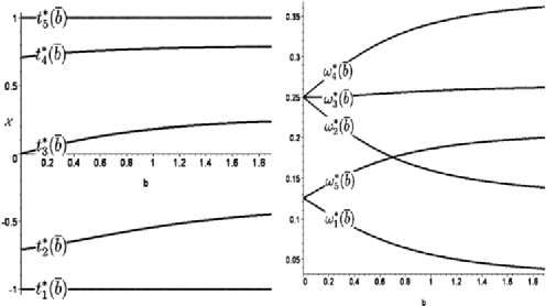
Figure 1: The support points (left panel) and weights (right panel) of the $T$-optimal design for discriminating between a polynomial of degree $3$ and $5$ for various values of $\bar{b}=1/b\in[0,1.894]$.

and this process is continued in order to determine the vector $\Theta^{*}(\bar{b})$ for any value $\bar{b}\in[0,1.894]$. The support points and weights are depicted in Figure 1 as a function of the parameter $\bar{b}=1/b=\theta_{1n}/\theta_{1n-1}$. Note that in all cases $b\neq 0$ the $T$-optimal design for discriminating between a polynomial of degree $5$ and $3$ is supported at $5$ points.

5 Concluding remarks and further discussion

In this paper we have determined $T$-optimal designs for discriminating between two rival polynomial regression models of degree $n-2$ and $n$. To the best of our knowledge these results provide the first analytic solution of a $T$-optimal discriminating design problem with an arbitrary number of parameters in the regression model.

It should be pointed out that the results depend on the ratio of the coefficients of the terms $x^{n-1}$ and $x^{n}$ in the polynomial of larger degree, which is a well-known feature of the $T$-optimality criterion. Therefore the designs derived here are local in the sense of Chernoff (1953). Usually locally optimal designs serve as a benchmark for commonly used designs, as demonstrated in the example in the Introduction. Moreover, locally optimal designs form the basis for more sophisticated design strategies, which require less knowledge about the model parameters such as Bayesian or standardized maximin optimality criteria [see Chaloner and Verdinelli (1995) or Dette (1997), among others]. This extension was already mentioned in the pioneering work of Atkinson and Fedorov (1975a, 1975b) and we conclude this paper with a brief discussion of a first explicit result on maximin $T$-optimal designs for the polynomial regression models.

To be precise, consider the situation where the ratio $b=\theta_{1,n-1}/\theta_{1,n}$ cannot be exactly specified, but prior knowledge suggests that $b\in I$ for some interval $I\subset\mathbb{R}$. Without loss of generality, assume $\theta_{1,n}=1$; then following Atkinson and Fedorov (1975a), a maximin optimal discriminating design maximizes the expression

$$\inf_{b\in I}\inf_{\theta_{2}\in\mathbb{R}^{n-1}}\int^{1}_{-1}\Biggl{(}x^{n}+bx^{n-1}+\sum^{n-2}_{j=0}\theta_{2,j}x^{j}\Biggr{)}^{2}\,d\xi(x).$$ (21)

The following result provides a solution of this optimal design problem for specific intervals $I\subset\mathbb{R}$.

Theorem 5.1

(a) If $I=\mathbb{R}$, the maximin $T$-optimal discriminating design is given by

$$\xi^{*}_{MM}=\pmatrix{t^{*}_{0}&t^{*}_{1}&\cdots&t^{*}_{n-1}&t^{*}_{n}\vspace*{2pt}\cr\dfrac{1}{2n}&\dfrac{1}{n}&\cdots&\dfrac{1}{n}&\dfrac{1}{2n}},$$ (22)

where the support points are defined by

$$t^{*}_{i}=\cos\biggl{(}\frac{n-i}{n}\pi\biggr{)},\qquad i=0,\ldots,n.$$

(b) Assume that $I=(-\infty,-b_{0}]$ or $I=[b_{0},\infty)$. If $b_{0}\geq 0$, then the maximin $T$-optimal discriminating design coincides with the $T$-optimal discriminating design determined in Sections 3 and 4 for the value $b=b_{0}$.

In particular, if $b_{0}=0$, then all designs specified in Theorem 3.1 are maximin $T$-optimal discriminating designs.

In order to prove part (a), note that for $I=\mathbb{R}$ criterion (21) reduces to

$$\sup_{\xi}\inf_{\theta\in\mathbb{R}^{n}}\int^{1}_{-1}\Biggl{(}x^{n}+\sum^{n-1}_{j=0}\theta_{2,n-1}x^{j}\Biggr{)}^{2}\,d\xi(x),$$

which corresponds to the $T$-optimal discriminating design problem for a polynomial of degree $n$ and $n-1$. By the results in Dette and Titoff (2009), the solution of this problem coincides with the $D_{1}$-optimal design, which is given by (22) [see Studden (1980)].

For a proof of part (b), observe that

$$\sup_{\xi}\inf_{b\in I}\sup_{\theta_{2}\in\mathbb{R}^{n-1}}\int^{1}_{-1}\Biggl{(}x^{n}+bx^{n-1}+\sum^{n-2}_{j=0}\theta_{2,j}x^{j}\Biggr{)}^{2}\,d\xi(x)$$

$$\qquad=\inf_{b\in I}\sup_{\xi}\sup_{\theta_{2}\in\mathbb{R}^{n-1}}\int^{1}_{-1}\Biggl{(}x^{n}+bx^{n-1}+\sum^{n-2}_{j=0}\theta_{2,j}x^{j}\Biggr{)}^{2}\,d\xi(x)=:\inf_{b\in I}R(b),$$

where the last equality defines the function $R$ in an obvious manner. We now consider the case $I=[b_{0},\infty)$ with $b_{0}\geq 0$ and show that the function $R$ is increasing on $\mathbb{R}^{+}$, which implies

$$\inf_{b\in I}R(b)=R(b_{0})$$ (23)

and proves the assertion for the case $I=[b_{0},\infty)$. Recall the definition of $b^{*}=n$ $\tan^{2}(\pi/2n)$ in (6); then the proof of Theorem 3.1 shows that for $\in(0,b^{*}]$

$$R(b)=\biggl{(}1+\frac{b}{n}\biggr{)}^{2n}\frac{1}{2^{2n-2}},$$

which is obviously increasing with respect to the argument $b$. If $R$ would be not increasing on the remaining region $\mathbb{R}^{+}\setminus(0,b^{*}]$, then there would exist real numbers $b_{2}>b_{1}>b^{*}$, such that $R(b_{1})=R(b_{2})$ with corresponding extremal polynomials

$$L_{i}(x)=x^{n}+b_{i}x^{n-1}+q^{T}_{i}\bar{f}(x),\qquad i=1,2,$$

where $\bar{f}(x)=(1,x,\ldots,x^{n-2})^{T}$ and

$$q_{i}=\mathop{\arg\min}_{q\in\mathbb{R}^{n-1}}\int^{1}_{-1}\bigl{(}x^{n}+b_{i}x^{n-1}+q^{T}\bar{f}(x)\bigr{)}^{2}\,d\xi(x).$$

This yields

$${\sup_{x\in[-1,1]}}|L_{1}(x)|={\sup_{x\in[-1,1]}}|L_{2}(x)|=\sqrt{R(b_{1})}=\sqrt{R(b_{2})}.$$

By the discussion in Section 4, the polynomials $L_{1},L_{2}$ can be chosen such that they coincide at the boundary points of the interval $[-1,1]$ (note that for $b>b^{*}$ the support of the optimal discriminating design always contains both boundary points $-1$ and $1$). Therefore a simple argument shows that there exist $n-2$ other points in the interior of the interval $(-1,1)$, where the polynomials must coincide. Consequently, $L_{1}(\tilde{t}_{j})=L_{2}(\tilde{t}_{j})$ for $n$ points $\tilde{t}_{1},\ldots,\tilde{t}_{n}\in[-1,1]$, which shows that the polynomials are identical. This yields $b_{1}=b_{2}$, and because of this contradiction the monotonicity of the function $R$ has been established, which proves (23) and part (b) in the case $I=[b_{0},\infty)$. The remaining case $I=(-\infty,-b_{0}]$ can be proved by similar arguments, and the details are omitted for the sake of brevity.

Theorem 5.1 provides the solution to maximin $T$-optimal discriminating design problems for specific intervals $I\subset\mathbb{R}$. In particular, it identifies the worst case as a boundary point of the interval under investigation using the monotonicity of the criterion with respect to $b$. This property, which appears in many minimax- or maximin optimal design problems, has been criticized by Dette (1997). This author recommends Bayesian or standardized maximin optimality criteria, which reflect the different sizes of the optimality criteria for different values of $b$ in a more reasonable way. The determination of $T$-optimal discriminating designs with respect to these criteria is substantially harder and a challenging problem for future research.

Appendix: Proof of identities (12) and (16)

Note that the identities in (12) and (16) can be written in the form

$$\sum^{n}_{i=1}t^{*k}_{i}(b)(-1)^{i}\omega^{*}_{i}=0,\qquad k=0,1,\ldots,n-2,$$ (1)

where $t^{*}_{i}(0)=\cos(\frac{i\pi}{n})=x_{i}$. We will prove that these equalities hold for any real number $b$. Since

$$\quad t^{*k}_{i}(b)=\sum^{k}_{j=0}a_{j}\cos\biggl{(}\frac{ji\pi}{n}\biggr{)},\qquad i=0,1,\ldots,n,k=0,1,\ldots,n-2,$$ (2)

for some coefficients $a_{j}=a_{j}(b)$ $(j=0,1,\ldots,k)$ the identities in (1) follow from

$$\sum^{n}_{i=1}(-1)^{i}\cos\biggl{(}\frac{ki\pi}{n}\biggr{)}\omega^{*}_{i}=0,\qquad k=0,1,\ldots,n-2.$$ (3)

In order to prove (3), consider first the case $k=0,n=2s$ for some $s$, where the left-hand side of (3) reduces to

$$\sum_{i=1}^{n}\omega_{i}^{*}(-1)^{i} = \frac{1}{n}\Biggl{[}\sum_{i=1}^{s-1}\biggl{[}\biggl{(}1-\cos\biggl{(}\frac{i\pi}{n}\biggr{)}\biggr{)}(-1)^{i}+\biggl{(}1+\cos\biggl{(}\frac{i\pi}{n}\biggr{)}\biggr{)}(-1)^{i}\biggr{]}$$

$$\hskip 195.6pt{}+(-1)^{s}+1\Biggr{]}$$

$$= \frac{1}{n}\Biggl{[}\sum_{i=1}^{s-1}2(-1)^{i}+(-1)^{s}+1\Biggr{]}=0,$$

which proves (3). If $k=0,n=2s+1$, we get

$$\sum_{i=1}^{n}\omega_{i}^{*}(-1)^{i} = \frac{1}{n}\Biggl{[}\sum_{i=1}^{s}\biggl{[}\biggl{(}1-\cos\biggl{(}\frac{i\pi}{n}\biggr{)}\biggr{)}(-1)^{i}-\biggl{(}1+\cos\biggl{(}\frac{i\pi}{n}\biggr{)}\biggr{)}(-1)^{i}\biggr{]}+(-1)\Biggr{]}$$

$$= \frac{1}{n}\Biggl{[}2\sum_{i=1}^{s}\cos\biggl{(}\frac{i\pi}{n}\biggr{)}(-1)^{i+1}-1\Biggr{]}$$

$$= \frac{1}{n}\biggl{[}1-\frac{\cos[{\pi(1+2(n+1)s)}/({2n})]}{\cos({\pi}/({2n}))}-1\biggr{]}$$

$$= -\frac{1}{n}\frac{\cos({(2s+1)\pi}/{2})}{\cos({\pi}/({2n}))}=0,$$

where the third identity follows by standard results for trigonometrical summation [see, e.g., Jolley (1961), formula (428)]. This proves (3) for the case $k=0,n=2s+1$. Now consider the case of even $n,n=2s$ for some odd $s$, $s=2l-1$ and $k$ of the form $k=2(2r-1)$. In this case the left-hand side of (3) reduces to

$$\frac{1}{n}\Biggl{[}\sum_{i=1}^{s-1}\biggl{[}\biggl{(}1-\cos\biggl{(}\frac{i\pi}{n}\biggr{)}\biggr{)}+\biggl{(}1+\cos\biggl{(}\frac{i\pi}{n}\biggr{)}\biggr{)}\biggr{]}(-1)^{i}\cos\biggl{(}\frac{ki\pi}{n}\biggr{)}$$

$$\hskip 143.0pt{}+(-1)^{s}\cos\biggl{(}\frac{k\pi}{2}\biggr{)}+\cos(k\pi)\Biggr{]}$$

$$\qquad=\frac{1}{n}\Biggl{[}2\sum_{i=1}^{s-1}(-1)^{i}\cos\biggl{(}\frac{ki\pi}{n}\biggr{)}+(-1)^{s}\cos\biggl{(}\frac{k\pi}{2}\biggr{)}+\cos(k\pi)\Biggr{]}$$

$$\qquad=\frac{1}{n}\biggl{\{}\biggl{(}\cos\biggl{(}\frac{k\pi}{4s}\biggr{)}\biggr{)}^{-1}\biggl{[}\cos\biggl{(}\frac{\pi k}{4s}-\pi\biggr{)}+\cos\biggl{(}\frac{\pi k}{4s}+\frac{\pi}{2}(k+2s-2)\biggr{)}\biggr{]}+2\biggr{\}}$$

$$\qquad=\frac{1}{n}\{(-1)+(-1)^{2s-1}+2\}=0,$$

where we have again used well-known results on trigonometric summation [see Jolley (1961), formula (428)]. Therefore we obtain equality (3) in the case $n=2s,s=2l-1$ and $k=2(2r-1)$. The other cases can be proved in a similar way, and the details are omitted for the sake of brevity.

References

- Achiezer (1956) {bbook}[auto:STB—2012/01/18—07:48:53] \bauthor\bsnmAchiezer, \bfnmN. I.\binitsN. I. (\byear1956). \btitleTheory of Approximation. \bpublisherUngar, \baddressNew York. \bptokimsref \endbibitem
- Asprey and Macchietto (2000) {barticle}[auto:STB—2012/01/18—07:48:53] \bauthor\bsnmAsprey, \bfnmS. P.\binitsS. P. and \bauthor\bsnmMacchietto, \bfnmS.\binitsS. (\byear2000). \btitleStatistical tools for optimal dynamic model building. \bjournalComputers and Chemical Engineering \bvolume24 \bpages1261–1267. \bptokimsref \endbibitem
- Atkinson (2010) {bmisc}[auto:STB—2012/01/18—07:48:53] \bauthor\bsnmAtkinson, \bfnmA. C.\binitsA. C. (\byear2010). \bhowpublishedThe non-uniqueness of some designs for discriminating between two polynomial models in one variablel. In mODa 9, Advances in Model-Oriented Design and Analysis (A. Giovagnoli, A. C. Atkinson, B. Torsney and C. May, eds.) 9–16. Physica, Heidelberg. \bptokimsref \endbibitem
- Atkinson, Bogacka and Bogacki (1998) {barticle}[auto:STB—2012/01/18—07:48:53] \bauthor\bsnmAtkinson, \bfnmA. C.\binitsA. C., \bauthor\bsnmBogacka, \bfnmB.\binitsB. and \bauthor\bsnmBogacki, \bfnmM. B.\binitsM. B. (\byear1998). \btitle- and -optimum designs for the kinetics of a reversible chemical reaction. \bjournalChemometrics and Intelligent Laboratory Systems \bvolume43 \bpages185–198. \bptokimsref \endbibitem
- Atkinson and Fedorov (1975a) {barticle}[mr] \bauthor\bsnmAtkinson, \bfnmA. C.\binitsA. C. and \bauthor\bsnmFedorov, \bfnmV. V.\binitsV. V. (\byear1975a). \btitleThe design of experiments for discriminating between two rival models. \bjournalBiometrika \bvolume62 \bpages57–70. \bidissn=0006-3444, mr=0370955 \bptokimsref \endbibitem
- Atkinson and Fedorov (1975b) {barticle}[mr] \bauthor\bsnmAtkinson, \bfnmA. C.\binitsA. C. and \bauthor\bsnmFedorov, \bfnmV. V.\binitsV. V. (\byear1975b). \btitleOptimal design: Experiments for discriminating between several models. \bjournalBiometrika \bvolume62 \bpages289–303. \bidissn=0006-3444, mr=0381163 \bptokimsref \endbibitem
- Chaloner and Verdinelli (1995) {barticle}[mr] \bauthor\bsnmChaloner, \bfnmKathryn\binitsK. and \bauthor\bsnmVerdinelli, \bfnmIsabella\binitsI. (\byear1995). \btitleBayesian experimental design: A review. \bjournalStatist. Sci. \bvolume10 \bpages273–304. \bidissn=0883-4237, mr=1390519 \bptokimsref \endbibitem
- Chernoff (1953) {barticle}[mr] \bauthor\bsnmChernoff, \bfnmHerman\binitsH. (\byear1953). \btitleLocally optimal designs for estimating parameters. \bjournalAnn. Math. Statist. \bvolume24 \bpages586–602. \bidissn=0003-4851, mr=0058932 \bptokimsref \endbibitem
- Denisov, Fedorov and Khabarov (1981) {bincollection}[auto:STB—2012/01/18—07:48:53] \bauthor\bsnmDenisov, \bfnmV. I.\binitsV. I., \bauthor\bsnmFedorov, \bfnmV. V.\binitsV. V. and \bauthor\bsnmKhabarov, \bfnmV. I.\binitsV. I. (\byear1981). \btitleTchebysheff approximation in problems of constructing asymptotic locally optimal designs for discriminating regression experiments. In \bbooktitleProblems in Cibernetics (Voprosy Kibernetiki in Russian), Linear and Non-Linear Parametrization in Optimal Design (\beditor\bfnmV.\binitsV. \bsnmFedorov and \beditor\bfnmV.\binitsV. \bsnmNalimov, eds.) \bpages3. \bpublisherAkademiya Nauk RSFSR, Nauchnyj Sovet po Kompleksnoj Probleme Kibernetika, \baddressMoskva. \bptokimsref \endbibitem
- Dette (1994) {barticle}[mr] \bauthor\bsnmDette, \bfnmHolger\binitsH. (\byear1994). \btitleDiscrimination designs for polynomial regression on compact intervals. \bjournalAnn. Statist. \bvolume22 \bpages890–903. \biddoi=10.1214/aos/1176325501, issn=0090-5364, mr=1292546 \bptokimsref \endbibitem
- Dette (1995) {barticle}[mr] \bauthor\bsnmDette, \bfnmHolger\binitsH. (\byear1995). \btitleOptimal designs for identifying the degree of a polynomial regression. \bjournalAnn. Statist. \bvolume23 \bpages1248–1266. \biddoi=10.1214/aos/1176324708, issn=0090-5364, mr=1353505 \bptokimsref \endbibitem
- Dette (1997) {barticle}[mr] \bauthor\bsnmDette, \bfnmHolger\binitsH. (\byear1997). \btitleDesigning experiments with respect to “standardized” optimality criteria. \bjournalJ. Roy. Statist. Soc. Ser. B \bvolume59 \bpages97–110. \bidissn=0035-9246, mr=1436556 \bptokimsref \endbibitem
- Dette and Haller (1998) {barticle}[mr] \bauthor\bsnmDette, \bfnmHolger\binitsH. and \bauthor\bsnmHaller, \bfnmGerd\binitsG. (\byear1998). \btitleOptimal designs for the identification of the order of a Fourier regression. \bjournalAnn. Statist. \bvolume26 \bpages1496–1521. \biddoi=10.1214/aos/1024691251, issn=0090-5364, mr=1647689 \bptokimsref \endbibitem
- Dette, Melas and Pepelyshev (2004) {barticle}[mr] \bauthor\bsnmDette, \bfnmHolger\binitsH., \bauthor\bsnmMelas, \bfnmViatcheslav B.\binitsV. B. and \bauthor\bsnmPepelyshev, \bfnmAndrey\binitsA. (\byear2004). \btitleOptimal designs for estimating individual coefficients in polynomial regression—a functional approach. \bjournalJ. Statist. Plann. Inference \bvolume118 \bpages201–219. \biddoi=10.1016/S0378-3758(02)00397-X, issn=0378-3758, mr=2015229 \bptokimsref \endbibitem
- Dette and Titoff (2009) {barticle}[mr] \bauthor\bsnmDette, \bfnmHolger\binitsH. and \bauthor\bsnmTitoff, \bfnmStefanie\binitsS. (\byear2009). \btitleOptimal discrimination designs. \bjournalAnn. Statist. \bvolume37 \bpages2056–2082. \biddoi=10.1214/08-AOS635, issn=0090-5364, mr=2533479 \bptokimsref \endbibitem
- Fedorov (1980) {bincollection}[mr] \bauthor\bsnmFedorov, \bfnmV.\binitsV. (\byear1980). \btitleDesign of model testing experiments. In \bbooktitleSymposia Mathematica, Vol. XXV (Conf., INDAM, Rome, 1979) \bpages171–180. \bpublisherAcademic Press, \baddressLondon. \bidmr=0618870 \bptnotecheck year\bptokimsref \endbibitem
- Fedorov and Khabarov (1986) {barticle}[mr] \bauthor\bsnmFedorov, \bfnmV.\binitsV. and \bauthor\bsnmKhabarov, \bfnmV.\binitsV. (\byear1986). \btitleDuality of optimal designs for model discrimination and parameter estimation. \bjournalBiometrika \bvolume73 \bpages183–190. \biddoi=10.1093/biomet/73.1.183, issn=0006-3444, mr=0836446 \bptokimsref \endbibitem
- Foo and Duffull (2011) {bmisc}[auto:STB—2012/01/18—07:48:53] \bauthor\bsnmFoo, \bfnmL. K.\binitsL. K. and \bauthor\bsnmDuffull, \bfnmS.\binitsS. (\byear2011). \bhowpublishedOptimal design of pharmacokinetic–pharmacodynamic studies. In Pharmacokinetics in Drug Development, Advances and Applications 3 (P. L. Bonate and D. R. Howard, eds.) 175–194. Springer, Berlin. \bptokimsref \endbibitem
- Hill (1978) {barticle}[auto:STB—2012/01/18—07:48:53] \bauthor\bsnmHill, \bfnmP. D.\binitsP. D. (\byear1978). \btitleA review of experimental design procedures for regression model discrimination. \bjournalTechnometrics \bvolume20 \bpages15–21. \bptokimsref \endbibitem
- Hunter and Reiner (1965) {barticle}[mr] \bauthor\bsnmHunter, \bfnmWilliam G.\binitsW. G. and \bauthor\bsnmReiner, \bfnmAlbey M.\binitsA. M. (\byear1965). \btitleDesigns for discriminating between two rival models. \bjournalTechnometrics \bvolume7 \bpages307–323. \bidissn=0040-1706, mr=0192615 \bptokimsref \endbibitem
- Jolley (1961) {bbook}[mr] \bauthor\bsnmJolley, \bfnmL. B. W.\binitsL. B. W. (\byear1961). \btitleSummation of Series, \bedition2nd revised ed. \bpublisherDover, \baddressNew York. \bidmr=0134458 \bptokimsref \endbibitem
- Kiefer (1974) {barticle}[mr] \bauthor\bsnmKiefer, \bfnmJ.\binitsJ. (\byear1974). \btitleGeneral equivalence theory for optimum designs (approximate theory). \bjournalAnn. Statist. \bvolume2 \bpages849–879. \bidissn=0090-5364, mr=0356386 \bptokimsref \endbibitem
- Melas (2006) {bbook}[mr] \bauthor\bsnmMelas, \bfnmViatcheslav B.\binitsV. B. (\byear2006). \btitleFunctional Approach to Optimal Experimental Design. \bseriesLecture Notes in Statistics \bvolume184. \bpublisherSpringer, \baddressNew York. \bidmr=2193670 \bptokimsref \endbibitem
- Song and Wong (1999) {barticle}[mr] \bauthor\bsnmSong, \bfnmDale\binitsD. and \bauthor\bsnmWong, \bfnmWeng Kee\binitsW. K. (\byear1999). \btitleOn the construction of -optimal designs. \bjournalStatist. Sinica \bvolume9 \bpages263–272. \bidissn=1017-0405, mr=1678893 \bptokimsref \endbibitem
- Spruill (1990) {barticle}[mr] \bauthor\bsnmSpruill, \bfnmM. C.\binitsM. C. (\byear1990). \btitleGood designs for testing the degree of a polynomial mean. \bjournalSankhyā Ser. B \bvolume52 \bpages67–74. \bidissn=0581-5738, mr=1178893 \bptokimsref \endbibitem
- Stigler (1971) {barticle}[auto:STB—2012/01/18—07:48:53] \bauthor\bsnmStigler, \bfnmS.\binitsS. (\byear1971). \btitleOptimal experimental design for polynomial regression. \bjournalJ. Amer. Statist. Assoc. \bvolume66 \bpages311–318. \bptokimsref \endbibitem
- Studden (1980) {barticle}[mr] \bauthor\bsnmStudden, \bfnmW. J.\binitsW. J. (\byear1980). \btitle-optimal designs for polynomial regression using continued fractions. \bjournalAnn. Statist. \bvolume8 \bpages1132–1141. \bidissn=0090-5364, mr=0585711 \bptokimsref \endbibitem
- Studden (1982) {barticle}[mr] \bauthor\bsnmStudden, \bfnmW. J.\binitsW. J. (\byear1982). \btitleSome robust-type -optimal designs in polynomial regression. \bjournalJ. Amer. Statist. Assoc. \bvolume77 \bpages916–921. \bidissn=0162-1459, mr=0686418 \bptokimsref \endbibitem
- Szegő (1975) {bbook}[mr] \bauthor\bsnmSzegő, \bfnmGábor\binitsG. (\byear1975). \btitleOrthogonal Polynomials, \bedition4th ed. \bseriesAmerican Mathematical Society, Colloquium Publications \bvolumeXXIII. \bpublisherAmer. Math. Soc., \baddressProvidence, RI. \bidmr=0372517 \bptokimsref \endbibitem
- Tommasi and López-Fidalgo (2010) {barticle}[mr] \bauthor\bsnmTommasi, \bfnmC.\binitsC. and \bauthor\bsnmLópez-Fidalgo, \bfnmJ.\binitsJ. (\byear2010). \btitleBayesian optimum designs for discriminating between models with any distribution. \bjournalComput. Statist. Data Anal. \bvolume54 \bpages143–150. \biddoi=10.1016/j.csda.2009.07.022, issn=0167-9473, mr=2558465 \bptokimsref \endbibitem
- Uciński and Bogacka (2005) {barticle}[mr] \bauthor\bsnmUciński, \bfnmDariusz\binitsD. and \bauthor\bsnmBogacka, \bfnmBarbara\binitsB. (\byear2005). \btitle-optimum designs for discrimination between two multiresponse dynamic models. \bjournalJ. R. Stat. Soc. Ser. B Stat. Methodol. \bvolume67 \bpages3–18. \biddoi=10.1111/j.1467-9868.2005.00485.x, issn=1369-7412, mr=2136636 \bptokimsref \endbibitem
- Wiens (2009) {barticle}[mr] \bauthor\bsnmWiens, \bfnmDouglas P.\binitsD. P. (\byear2009). \btitleRobust discrimination designs. \bjournalJ. R. Stat. Soc. Ser. B Stat. Methodol. \bvolume71 \bpages805–829. \biddoi=10.1111/j.1467-9868.2009.00711.x, issn=1369-7412, mr=2750096 \bptokimsref \endbibitem
- Wiens (2010) {barticle}[mr] \bauthor\bsnmWiens, \bfnmDouglas P.\binitsD. P. (\byear2010). \btitleRobustness of design for the testing of lack of fit and for estimation in binary response models. \bjournalComput. Statist. Data Anal. \bvolume54 \bpages3371–3378. \biddoi=10.1016/j.csda.2009.03.001, issn=0167-9473, mr=2727759 \bptokimsref \endbibitem