Spontaneously induced general relativity with holographic interior and general exterior

Abstract

We study the spontaneously induced general relativity (GR) from the scalar-tensor gravity. We demonstrate by numerical methods that a novel inner core can be connected to the Schwarzschild exterior with cosmological constants and any sectional curvature. Deriving an analytic core metric for a general exterior, we show that all the nontrivial features of the core, including the locally holographic entropy packing, are universal for the general exterior in static spacetimes. We also investigate whether the f(R) gravity can accommodate the nontrivial core.

1 Introduction

Recently, by studying the scalar-tensor gravity, Davidson and Gurwich [1] found an interesting metric, for which the exterior Schwarzschild solution of GR is spontaneously induced by a phase transition which occurs precisely at the would-have-been event horizon (see earlier discussion on the horizon phase transition [2]), and the interior core is characterized by some nontrivial features. For instance, the core has a vanishing spatial volume. This provides a simple but direct explanation of the well-known problem: why the BH entropy is not proportional to the volume of the system as usual. Note that the volume of normal BH can not be well-defined [3], partially because the r$\leftrightarrow$t signature flip, but in the current situation, it makes better since no such flip. Moreover, compared with the Schwarzschild BH, the Komar mass [4] within the core is well defined (non-singular and positive). Then the Smarr formula [5] can be extended to any inner sphere on which the area-entropy relation is extracted. It was argued that this provides a local realization of maximal entropy packing and a new way of Nature’s ultimate information storage. In Ref. [6], Davidson further designed a discrete holographic shell model to capture the holographic entropy packing inside BHs. It is interesting to see that even the logarithmic correction can be recovered.

The Davidson-Gurwich (DG) horizon phase transition has been also found in the case with the Reissner-Nordstrom (RN) exterior [7]. A natural problem is whether the phase transition can exist for a more general exterior. Respecting the celebrated holographic correspondence between the supergravity in Anti-de Sitter (AdS) space and conformal field theory (CFT) on the boundary [8], one would most like to ask whether the locally holographic entropy packing can be present inside Schwarzschild-AdS BHs. Moreover, one may also concern about the realization of the DG horizon phase transition in the asymptotically dS exterior, since the accelerated expansion of present universe could be derived by the positive cosmological constant and the earlier universe is well represented by dS-like exponentially inflationary phase.

In this paper, by choosing a special scalar potential, we will demonstrate the DG horizon phase transition with the Schwarzschild-dS/AdS exterior by numerical methods. With the mind that the AdS/CFT correspondence usually focuses on the CFT in the flat spacetime, we will consider the spacetime with any sectional curvature. Furthermore, we will derive a general form of the core metric by a new (semi-)analytic method and check the nontrivial features.

On the other hand, in Refs. [1, 7], it was suggested that the DG phase transition can also be found in a simple theory of $f(R)$ gravity with the square curvature correction. However, we will show that there is a subtle problem in the suggestion, that is, a precondition to the equivalence between the scalar-tensor gravity and $f(R)$ gravity is not satisfied directly for the core metric.

2 A special scalar-tensor gravity

Consider the scalar-tensor gravity without the kinetic term

$$S=\frac{1}{16\pi}\int\left[\phi R-V(\phi)\right]\sqrt{-g}~{}d^{4}x+S_{M}.$$ (1)

The gravitational field equations and the equation of motion for the scalar field can be derived by varying this action with respect to $g_{\mu\nu}$ and $\phi$:

$$\phi G_{ab}-\nabla_{a}\nabla_{b}\phi+g_{ab}\nabla^{c}\nabla_{c}\phi+\frac{1}{2}g_{ab}V(\phi)-8\pi T_{ab}=0,$$ (2)

$$R-\frac{dV}{d\phi}=0,$$ (3)

where $T_{ab}$ denotes the energy-momentum tensor of matter.

Refs. [1, 7] consider the 4-dimensional static spacetime with the spherical symmetry. In this paper, we will extend it to other topological cases, which is interesting especially in the asymptotically AdS space. We write the line element as

$$ds^{2}=-e^{\nu(r)}dt^{2}+e^{\lambda(r)}dr^{2}+r^{2}d\Omega^{2},$$ (4)

where $\Omega$ expresses the surface with the constant sectional curvature $k=0,\pm 1$.

To be consistent with the GR outside the core, the potential $V(\phi)$ has been chosen as [1, 7]

$$V(\phi)=\frac{3}{2a}\left(\phi-\frac{1}{G}\right)^{2},$$ (5)

where the value of $a$ can be made as small as necessary to be compatible with Solar System tests. But for spontaneously inducing the GR with the cosmological constant $\Lambda$, we will modify the potential to

$$V(\phi)=\frac{3}{2a}\left(\phi-\frac{1}{G}\right)^{2}+4\Lambda\left(\phi-\frac{1}{G}\right)+\frac{2\Lambda}{G}.$$ (6)

Note that the second term in the RHS of Eq. (6) is added so that Eq. (3) can be equivalent to the contracted Einstein equation $R-4\Lambda=0$ when $\phi\rightarrow 1/G$ outside the core.

3 Horizon phase transition: numerical method

To obtain the master equations that having a nontrivial solution, one needs to solve $\nu^{\prime\prime}$ (the prime denotes the derivative with respect to $r$) from Eq. (3)

$$\nu^{\prime\prime}=\frac{1}{2r^{2}}\left[-4+4ke^{\lambda}-2e^{\lambda}r^{2}\frac{dV}{d\phi}+r\left(\lambda^{\prime}-\nu^{\prime}\right)(4+\nu^{\prime})\right],$$ (7)

and use it to cancel $\nu^{\prime\prime}$ in the field equation (2). Then the independent components of field equations can be reorganized as

$$\phi^{\prime\prime}-\frac{1}{2}\left(\nu^{\prime}+\lambda^{\prime}\right)\phi^{\prime}-\frac{1}{r}\left(\nu^{\prime}+\lambda^{\prime}\right)\phi=0,$$ (8)

$$\phi^{\prime\prime}+\frac{1}{2}\left(\nu^{\prime}-\lambda^{\prime}\right)\left(\phi^{\prime}-\frac{2}{r}\phi\right)-\frac{2}{r^{2}}\left(1-ke^{\lambda}\right)\phi-\frac{2}{3}e^{\lambda}\left(\phi\frac{dV}{d\phi}-\frac{1}{2}V\right)=0,$$ (9)

$$\phi^{\prime\prime}+\left[\frac{1}{2}\left(\nu^{\prime}-\lambda^{\prime}\right)+\frac{2}{r}\right]\phi^{\prime}-\frac{1}{3}e^{\lambda}\left(\phi\frac{dV}{d\phi}-2V\right)=0.$$ (10)

These three equations with the potential (6) are the master equations that we will solve. Here we have set $T_{b}^{a}=0$ for our aim.

Let us determine the boundary conditions of master equations. Consider the perturbation around a general exterior

$$\phi(r)=1+s\phi_{1}(r),\;\lambda(r)=-\log[g(r)+sL_{1}(r)],\;\nu(r)=\log[h(r)+sN_{1}(r)],$$

where $g$ and $h$ denote the metric components of general GR exterior, and the constant $s$ serves as a small expansion parameter. Substituting these perturbative solutions into Eq. (10), one can find a decoupled linear differential equation at leading order

$$\phi_{1}^{\prime\prime}+\frac{1}{2}\left(\frac{4}{r}+\frac{g^{\prime}}{g}+\frac{h^{\prime}}{h}\right)\phi_{1}^{\prime}-\frac{1}{g}(\frac{1}{a}-\frac{4}{3}\Lambda)\phi_{1}=0.$$

Now we specify the exterior as

$$g=h=k-\frac{2M}{r}\pm\frac{r^{2}}{L^{2}},$$

where we have set $G=1$ and $\Lambda=\mp 3/L^{2}$ for convenience. Note that the above/below branch refer to Schwarzschild-AdS/dS spacetimes. At large $r$, we get rid of the diverging term to stay with the converging tail

$$\phi_{1}\simeq r^{-\frac{3}{2}-\frac{5}{2}\sqrt{1\pm\frac{4L^{2}}{25a}}}.$$ (11)

Obviously, the small parameter $a$ should be positive/negative for negative/positive $\Lambda$. With the aid of $\phi_{1}$, one can obtain $L_{1}$ and $N_{1}$ from the remained master equations (8) and (9):

$$L_{1}\simeq\pm\frac{5}{2L^{2}}\left(1+\sqrt{1\pm\frac{4L^{2}}{25a}}\right)r^{\frac{1}{2}\left(1-5\sqrt{1\pm\frac{4L^{2}}{25a}}\right)},$$ (12)

$$N_{1}\simeq-\frac{5r}{2}\left(k-\frac{2M}{r}\right)\left(1+\sqrt{1\pm\frac{4L^{2}}{25a}}\right)r^{-\frac{5}{2}\left(1+\sqrt{1\pm\frac{4L^{2}}{25a}}\right)},$$ (13)

One should be careful that the term$\sim 2M/r$ in Eq. (13) is necessary for the case with $k=0$.

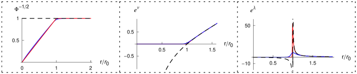
Figure 1: The configuration $e^{\lambda}$, $e^{\nu}$ and $\phi$ with $\Lambda<0$ and $k=1$. The parameter in scalar potential and the AdS radius are fixed as $a=0.1$ and $L=2$. The blue and red lines refer to the expansion parameters $s=0.1$ and $0.01$. The dashed lines depict the usual BH solutions with $s=0$.

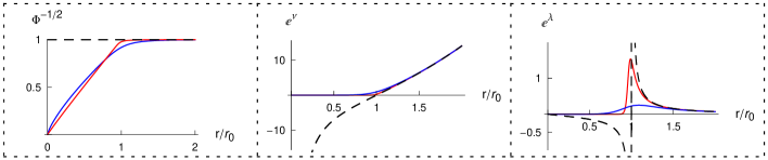
Figure 2: The configuration $e^{\lambda}$, $e^{\nu}$ and $\phi$ with $\Lambda<0$ and $k=0$. The parameters are set as $a=0.05$ and $L=1$. The blue and red lines refer to the expansion parameters $s=0.1$ and $0.01$. The dashed lines depict the usual BH solutions with $s=0$.

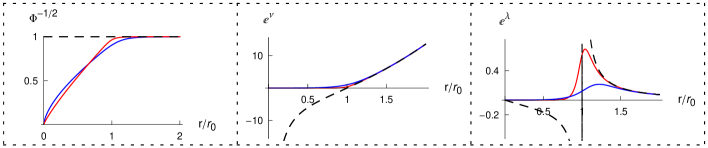
Figure 3: The configuration $e^{\lambda}$, $e^{\nu}$ and $\phi$ with $\Lambda<0$ and $k=-1$. The parameters are set as $a=0.01$ and $L=0.5$. The blue and red lines refer to the expansion parameters $s=0.1$ and $0.01$. The dashed lines depict the usual BH solutions with $s=0$.

Hereto, we can perform a full numerical integration. For convention, the horizon radius has been normalized to unity. Using Eqs. (11), (12) and (13) at some large enough distance as the boundary conditions, we produce Figs. 1, 2 and 3 for the configuration of $e^{\lambda}$, $e^{\nu}$ and $\phi$ with negative $\Lambda$ and different $k$, as well as Fig. 4 for the case of positive $\Lambda$. One can find that the exterior of topological-Schwarzschild-AdS BHs and Schwarzschild-dS is recovered at the $s\rightarrow 0$ limit, and the inner core differs conceptually from the interior of usual BHs with $s=0$ (see the dashed lines). We like to stress three characteristic features of the overall configuration: 1) $e^{\lambda}$ and $e^{\nu}$ are drastically suppressed inside the core; 2) there is no signature flip at the would-have-been horizon; and 3) three functions $e^{\lambda}$, $e^{\nu}$ and $\phi$ at the $s\rightarrow 0$ limit are all changed abruptly very near the would-have-been horizon, which manifests the horizon phase transition.

Moreover, one should be noted that the would-have-been horizon that connects the Schwarzschild-dS exterior is located at the cosmological horizon, instead of the event horizon in the cases of RN and Schwarzschild-AdS exterior. From Fig. (4), one can conclude that the total spacetime is dynamical since $t$ denotes the spacelike coordinate and $r$ is timelike.

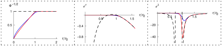
Figure 4: The configuration $e^{\lambda}$, $e^{\nu}$ and $\phi$ with $\Lambda>0$. The parameter in scalar potential and the dS radius are set as $a=-0.1$ and $L=1.5$. The blue and red lines refer to the expansion parameters $s=10^{-3}$ and $10^{-4}$. The dashed lines depict the usual BH solutions with $s=0$.

4 Analytic inner core

It this section, we will solve the master equations by a new analytic method. One can find that it is consistent with the numerical results and it is convenient to be used to check the nontrivial features of core in the next section.

4.1 General core metric with undetermined constants

By numerical inspection, we have shown that $e^{\lambda}$ is negligible inside the would-have-been horizon (see the first feature that we have stressed in above section). This suggests us to simplify the master equations by imposing $e^{\lambda}\rightarrow 0$ inside the core. With this in mind, the master equations can be translated into

$$\phi^{\prime\prime}=\phi^{\prime}\left(-\frac{1}{r}+\frac{\phi^{\prime}}{\phi}\right),\;\lambda^{\prime}=\frac{2\left(\phi^{2}+r\phi\phi^{\prime}+r^{2}\phi^{\prime 2}\right)}{r\phi\left(2\phi+r\phi^{\prime}\right)},\;\nu^{\prime}=-\frac{2\left(\phi+2r\phi^{\prime}\right)}{r\left(2\phi+r\phi^{\prime}\right)}.$$

The analytic solution can be obtained as follows

$$\phi=\gamma\left(\frac{r}{r_{0}}\right)^{-2+\epsilon},\;e^{\lambda}=\beta\left(\frac{r}{r_{0}}\right)^{\frac{6}{\epsilon}-6+2\epsilon},\;e^{\nu}=\alpha\left(\frac{r}{r_{0}}\right)^{\frac{6}{\epsilon}-4},$$ (14)

where $\alpha$, $\beta$, $\gamma$ and $\epsilon$ are the constants of integration. The scalar $r_{0}$ can be interpreted as the radius of the core because the core metric (14) can be self-consistent with the condition $e^{\lambda}\rightarrow 0$ for all $r<r_{0}$, if one imposes $0<\epsilon<<1$. However, the scale $r_{0}$ is fictitious at this stage since it can be absorbed into the coefficients $\alpha$, $\beta$, $\gamma$. The arbitrariness will be removed while we match the core metric with the exterior solution.

The form of core metric (14) with $k=1$ has been obtained for the matter being vacuum [1] or electromagnetic field [7]. Here we have shown that the core metric can be derived with any $k$ and without invoking the concrete scalar potential. Moreover, we note that Eq. (14) also can be derived using the equation (7) and the field equations with general matter content, provided that the matter satisfies $e^{\lambda}T_{b}^{a}\rightarrow 0$ inside the core.

4.2 Matching the core with a general exterior

In Ref. [7], an analytic method was proposed to fix the integration constants. This method solves field equations near the region of phase transition then matches the result to the core and the RN exterior, respectively. However, it seems difficult to extend the analytic method to more general exterior. On the other hand, we note that there is a more simple analytic method to solve differential equations, which directly matches two approximate solutions near two boundaries. Recently, this analytic method was introduced to understand the holographic superconductor [9, 10, 11]. For the case of $d\leq 5$ dimensional spacetimes, the analytic method can explain the qualitative features of superconductors and gives fairly good agreement with numerical results. A natural idea is to use this method to connect the core with the general exterior. Before doing that, we would like to introduce a problem about the selection of the matching point. In Ref. [9], the matching point is selected as the intermediate value $z_{m}=1/2$ between the range ($0<z<1$), but in fact, it could be rather arbitrary without changing the qualitative features. For the case of $d>5$, it was found [10] that the matching point should be chosen in an appropriate range ($z_{md}<z_{m}<1$), otherwise the behavior of holographic superconductor can not be imitated qualitatively. In our understanding, this means that the behavior of the exact solution is not smooth enough to be simulated by the direct matching in the whole range. Hence, one can suspect that for some differential equations which have very sharp peaks, the appropriate range of matching points is very small, and even no appropriate matching point can be found. In the following, one can find that we are just encountering both cases. Fortunately, we still can obtain correct results by a reasonable assumption.

At first, let us consider the matching of core metric $e^{\nu}$ and the general GR solution $h$. For convention, we will change the variable $r$ to $z=r_{0}/r$, thus $z=1$ means the would-have-been horizon. The smooth matching usually requires two functions at two boundaries and their derivatives can be connected at one point:

$$\left.\alpha\left(\frac{1}{z}\right)^{\frac{6}{\epsilon}-4}\right|_{z_{m}}=h(z_{m}),\;\left.\partial_{z}\left[\alpha\left(\frac{1}{z}\right)^{\frac{6}{\epsilon}-4}\right]\right|_{z_{m}}=\left.\partial_{z}h(z)\right|_{z_{m}},$$ (15)

which can be solved as

$$h(z_{m})=\left.\frac{z\epsilon h^{\prime}}{-6+4\epsilon}\right|_{z_{m}},$$ (16)

$$\alpha=\left.\frac{\left(\frac{1}{z}\right)^{3-\frac{6}{\epsilon}}\epsilon h^{\prime}}{-6+4\epsilon}\right|_{z_{m}}.$$ (17)

From Eq. (16) and Eq. (17), one can find that $h(z)$ should satisfy $\left|h(z_{m})\right|\ll 1$, $h^{\prime}(z_{m})/h(z_{m})<0$, and $\alpha/h(z_{m})>0$, because $\epsilon$ should be a very small positive number to suppress $e^{\lambda}$ and $e^{\nu}$, and there is no signature flip at the would-have-been horizon (see the first and second features which we have stressed in above section). This further means that the matching point is restricted at a very small range of $z_{m}\lesssim 1$. Expanding Eq. (16) near the horizon, we have

$$z_{m}=\frac{6-5\epsilon}{6-4\epsilon}+\mathcal{O}(z_{m}-1)^{2}.$$ (18)

Substituting Eq. (18) into Eq. (17) and using $0<\epsilon<<1$, we obtain

$$\alpha=-\frac{h^{\prime}(1)}{6e}\epsilon+\mathcal{O}(\epsilon)^{2},$$ (19)

where $e$ is the base of the natural logarithm.

Next, we will consider the matching of core metric $e^{\lambda}$ and the general GR solution $1/g$. We require the core metric and exterior solution can be connected at certain point, which leads to

$$\left.\frac{1}{\beta}\left(\frac{1}{z}\right)^{6-\frac{6}{\epsilon}-2\epsilon}\right|_{z_{m}}=g(z_{m}).$$ (20)

Naively, one might also require their derivatives connecting, which means

$$\left.\partial_{z}\left[\frac{1}{\beta}\left(\frac{1}{z}\right)^{6-\frac{6}{\epsilon}-2\epsilon}\right]\right|_{z_{m}}=\left.\partial_{z}g(z)\right|_{z_{m}}.$$ (21)

Combing Eq. (20) and Eq. (21), one can obtain

$$g(z_{m})=\left.\frac{z\epsilon g^{\prime}}{6-6\epsilon+2\epsilon^{2}}\right|_{z_{m}},$$ (22)

$$\beta=\left.\frac{2\left(\frac{1}{z}\right)^{7-\frac{6}{\epsilon}-2\epsilon}(3-3\epsilon+\epsilon^{2})}{\epsilon g^{\prime}}\right|_{z_{m}}.$$ (23)

If carrying out the similar analysis below Eq. (17), one can find that $g^{\prime}(z_{m})/g(z_{m})$ should be positive and the matching point should be located at $z_{m}\lesssim 1$. However, this result is conflicted with all the numerical solutions that we have known. Analyzing the analytic core metric (14) and Schwarzschild exterior for instance, one can find that Eq. (20) can be easily satisfied but Eq. (21) can not hold outside the horizon. This phenomenon is more clear if one considers the direct matching between $\phi=\gamma\left(\frac{r}{r_{0}}\right)^{-2+\epsilon}$ and the GR exterior $\phi=1$, since the derivative of $\gamma\left(\frac{r}{r_{0}}\right)^{-2+\epsilon}$ can not be vanishing unless $\gamma=0$. For fixing two integration constants $\beta$ and $\epsilon$, we would like to give up the smooth matching but expect to replace Eq. (21) with another new condition. Here we propose that $e^{\lambda}$, $e^{\nu}$ and $\phi$ can be matched at the same position. This is a natural ansatz since it implies that we are considering the phase transition which happens at the same position (see the third feature that we have stressed in above section). Thus, expanding Eq. (20) near the horizon and using Eq. (18), we have

$$\beta=-\frac{6}{g^{\prime}(1)e}\frac{1}{\epsilon}+\mathcal{O}(\epsilon)^{0}.$$ (24)

Similarly, in terms of Eq. (18) and

$$\left.\gamma\left(\frac{1}{z}\right)^{-2+\epsilon}\right|_{z_{m}}=1,$$ (25)

we can fix the integration constant as $\gamma\simeq 1$.

Several remarks are in order. Firstly, we stress that Eq. (19), Eq. (24) and $\gamma\simeq 1$ can be viable to a general exterior. The information of general exterior manifests in $h^{\prime}(1)$ and $g^{\prime}(1)$. Thus, in the next section, we can study the features of the core connecting a general exterior, while not restricted in a concrete BH. Secondly, the explicit expressions of $\alpha$, $\beta$ and $\gamma$ demonstrate that $r_{0}$ is the horizon radius indeed. Thirdly, we can recover the results obtained in Refs. [1, 7] for the Schwarzschild or RN exterior, up to a factor of the number $e$. Interestingly, the number $e$ will not affect any properties of the core, as we will show in next section. Fourthly, in the above, we treat three functions ($h$, $g$ and $\phi$) as independent functions. In fact, with the mind that there are only four constants of integration $\alpha$, $\beta$, $\gamma$ and $\epsilon$, one can not impose three functions and their derivatives connecting at the same time in general. To obtain the desired nontrivial core, one can select four conditions as we have done, namely, Eqs. (16), (17), (20), and (25). Nevertheless, we still have treated these functions as independent ones, because it suggests a simple but robust analytic method, which could be applicable to the case where the undetermined functions of some differential equations have enough constants of integration and the exact solutions do not satisfy all the conditions of the direct smooth matching. The key point is to find the reasonable alternative conditions.

At last, we write the general form of the core metric for any exterior solution

$$ds^{2}=-\frac{\epsilon r_{0}h^{\prime}(r_{0})}{6e}\left(\frac{r}{r_{0}}\right)^{\frac{6}{\epsilon}-4}dt^{2}+\frac{6}{\epsilon r_{0}g^{\prime}(r_{0})e}\left(\frac{r}{r_{0}}\right)^{\frac{6}{\epsilon}-6+2\epsilon}dr^{2}+r^{2}d\Omega^{2},$$ (26)

where we have recovered $r_{0}$ explicitly for later convention.

5 The nontrivial core features

In this section, we will check whether the different exterior, namely, the factors $h^{\prime}(r_{0})$ and $g^{\prime}(r_{0})$, and the number $e$ that characterizes our analytic method, will affect the nontrivial features of the core given in [1, 7]. Before doing that, it should be noted that the approach to the nontrivial features requires a static spacetime. For instance, the Killing vector will be involved, which is not well defined in a dynamic spacetime. So we will take into account the core with a general static exterior, which excludes the case of Schwarzschild-dS exterior.

5.1 Vanishing spatial volume

Associated with any surface $\Omega$ of radius $r$, the spatial volume is

$$V(r)=\Omega\int_{0}^{r}\sqrt{g_{rr}}r^{2}dr\simeq\sqrt{\frac{6\epsilon}{r_{0}g^{\prime}(r_{0})e}}\left(\frac{r}{r_{0}}\right)^{\frac{3}{\epsilon}}\frac{\Omega}{3}r_{0}^{3},$$ (27)

where we have used $\Omega$ to express the unit area of the surface $\Omega$. In contrast to the corresponding finite surface area $A(r)=\Omega r^{2}$, it is obvious that the spatial volume tends to vanish at the $\epsilon\rightarrow+0$ limit.

5.2 Constant temperature

The surface gravity of any surface inside the core can be calculated as

$$\kappa=\frac{1}{2}e^{-\lambda}\sqrt{e^{\lambda+\nu}}\nu^{\prime}=-\frac{1}{6}\left(\frac{r}{r_{0}}\right)^{-\epsilon}(2\epsilon-3)\sqrt{g^{\prime}(r_{0})h^{\prime}(r_{0})}\simeq\frac{1}{2}\sqrt{g^{\prime}(r_{0})h^{\prime}(r_{0})}.$$ (28)

One can find that $\kappa$ tends to be a constant from $r=r_{0}$ to the origin at $r=0$. Moreover, this constant is exactly identified as $2\pi$ the Hawking temperature of usual BHs. This suggests that the core is under thermodynamic equilibrium. The nontrivial feature of the core temperature can also be seen from the Rindler structure of the core:

$$ds_{in}^{2}=-\kappa^{2}\eta^{2}dt^{2}+d\eta^{2}+\left(\frac{3\kappa\eta^{2}}{\epsilon r_{0}}\right)^{\frac{3}{\epsilon}}r_{0}^{2}d\Omega^{2},$$ (29)

where the proper length coordinate is

$$\eta(r)=\int\sqrt{\beta\left(\frac{r}{r_{0}}\right)^{\frac{6}{\epsilon}-6+2\epsilon}}dr=\frac{\left(\frac{r}{r_{0}}\right)^{-2+\frac{3}{\epsilon}+\epsilon}\sqrt{\frac{6r_{0}}{\epsilon eg^{\prime}(r_{0})}}}{\left(\frac{3}{\epsilon}-2+\epsilon\right)}.$$ (30)

Thus, Hawking’s imaginary time periodicity can be recovered from Eq. (29). But unlike in the original GR BH, the Euclidean origin corresponds now to the center of $r=0$ rather than to $r=r_{0}$. By calculating the curvature scalar at leading order, for instance,

$$R^{\mu\nu}R_{\mu\nu}\simeq\left(\frac{r}{r_{0}}\right)^{-\frac{12}{\epsilon}+8+4\epsilon}2e^{2}g^{\prime}(r_{0})^{2}+\frac{2k^{2}}{r^{4}},$$

one should be noted that the origin is always the singularity of the general metric. This problem was expected [1, 7] to be solved by involving a more complicated Lagrangian or quantum effects.

5.3 Positive-definite mass

Consider the Komar mass [4]

$$m_{K}=\frac{1}{4\pi}\int_{\Sigma}d\Sigma_{\mu}\xi_{\nu}R^{\mu\nu},$$ (31)

where $\xi$ is the Killing vector and $\Sigma$ is a spatial volume with the boundary $\Omega$. One can prove that for any surface $\Omega$, it satisfies a geometric relation

$$m_{K}(r)=\frac{1}{4\pi}\kappa(r)A(r),$$ (32)

which can be reduced to the Smarr formula for usual BHs [5]. The Komar mass is meaningless in the interior of usual BHs, where $\kappa(r)$ and $m_{K}(r)$ can be negative and even negative infinite [1, 7]. Interestingly, however, $m_{K}(r)$ of the core metric (26) is finite and positive-definite as desired for the gravitational mass.

5.4 Freezing light ray

One can see that the radial light rays obey the null geodesics

$$r(t)=r_{in}e^{\pm t\left/\tilde{t}\right.},\ \tilde{t}=\frac{6r_{0}}{\epsilon\sqrt{g^{\prime}(r_{0})h^{\prime}(r_{0})}}.$$ (33)

Thus, for an observer at asymptotic distance, a light ray sent from some $r_{in}<r_{0}$ is very difficult to move even a small distance. In other words, it indicates that each layer of the core acts as an event horizon which freezes the light ray if one looks from the outside. It hence seems reasonable to associate the entropy on any inner surface to describe the lack of the information behind it.

5.5 Holographic entropy packing

With the mind that the surface gravity is constant inside the core, Eq. (32) suggests that every concentric inner surface of invariant surface area $A(r)$ carries a geometric fraction $A(r)/A(r_{0})$ of the total Komar mass enclosed by the would-have-been outer horizon, which also hints the entropy packing inside the would-have-been horizon. Furthermore, since the surface gravity can be exactly identified as $2\pi$ the Hawking temperature of usual BHs, one can rewrite the Smarr formula (32) as

$$m_{K}(r)=2T(r_{0})\left(S(r_{0})\frac{r^{2}}{r_{0}^{2}}\right).$$ (34)

Note that there does not exist an analogous formula for the interior of ordinary BHs. Taking Eq. (34) as a significant thermodynamic equality, one could regard the expression in the parenthesis in Eq. (34) as the entropy stored within an arbitrary inner surface

$$S(r)=S(r_{0})\frac{r^{2}}{r_{0}^{2}}=\frac{A(r)}{4}.$$ (35)

Interestingly, this is just the universal holographic entropy bound, and what is remarkable is that the bound is locally saturated.

Hereto, none of the features of the core which we have checked are influenced by the factors of the general exterior. Moreover, all the features also have not been affected by the number $e$ appeared in the core metric (26), which supports the effectiveness of our analytic method.

6 About the $f(R)$ gravity

In general, the $f(R)$ theory can be equivalent to the Brans–Dicke theory with the vanishing Brans–Dicke parameter, if the condition

$$\phi=f_{R}=\frac{df(R)}{dR},\;V=Rf_{R}-f$$ (36)

is satisfied [12]. Therefore, in Refs. [1, 7], it was suggested that the DG horizon phase transition can also be found in a simple $f(R)$ gravity with the square curvature correction

$$f=R+\frac{a}{6}R^{2},$$ (37)

since Eq. (37) and Eq. (5) satisfy Eq. (36). Actually, the equation of motion of scalar field (3) can be expressed as

$$R=\frac{3}{a}(\phi-1),$$

which is equivalent to the condition

$$\phi=f_{R}=1+\frac{a}{3}R.$$ (38)

However, one should be careful that, according to the metric ansatz (4), the field equations (2) (then the master equations) include three independent equations which are enough to determine three undetermined functions $\lambda$, $\nu$, and $\phi$. Thus, in general, the obtained solutions will not satisfy Eq. (38), which hence must be taken as an additional constraint. In the following, we will show both analytically and numerically that the solution with the DG horizon phase transition does not satisfy Eq. (38) indeed.

Using the analytic core metric (26) and $\phi\simeq\left(\frac{r}{r_{0}}\right)^{-2+\epsilon}$, one can calculate

$$f_{R}-\phi=1+\frac{a}{3}R-\phi=1+\frac{2ka}{3r^{2}}-\left(\frac{r}{r_{0}}\right)^{-2+\epsilon},$$ (39)

which obviously can not be vanishing in general. Fig. 5 gives the numerical check of Eq. (38). One can find that $f_{R}-\phi$ is not vanishing in general inside the core. In particular, it increases rapidly when the parameter $s$ declines.

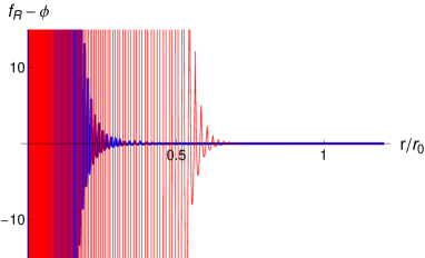
Figure 5: Check of the condition $f_{R}=\phi$ for the core with Schwarzschild exterior. The parameter $a=0.01$. The blue and red lines refer to $s=0.1$ and $0.01$.

Thus, it seems difficult to argue that the DG horizon phase transition can be found in the $f(R)$ gravity only because of the usual equivalence between the scalar-tensor gravity and $f(R)$ gravity.

7 Summary

In this paper, we have studied the scalar-tensor gravity without the kinetic term. Choosing a special scalar potential, we have shown by numerical methods that there is the DG horizon phase transition, which connects the topological-Schwarzschild-AdS or Schwarzschild-dS exterior with the inner core that differs conceptually from the interior of usual BHs. We also find an analytic expression of the core connecting a general exterior. We have checked that the static analytic core has the nontrivial features, including the vanishing spatial volume, constant temperature, positive-definitive Komar mass, the freezing light ray, and the locally holographic entropy packing. All these features are not changed by the factor of the general exterior. Our results suggest that the spontaneously induced GR with holographic interior could be viable for very general GR exterior in static spacetimes.

Comparing the solutions with and without the cosmological constants, one can find that the solution with Schwarzschild-dS exterior is very different with the one with Schwarzschild or RN exterior, that is, the would-have-been horizon that connects the Schwarzschild-dS exterior is located at the cosmological horizon, instead of the event horizon. On the other hand, this result is consistent with the solution with RN exterior, since the would-have-been horizons are both the outer horizons. The positive cosmological constant does not give the solution any qualitative difference. We expect that the holographic core with asymptotically AdS exterior might lead to some interesting results in the AdS/CFT correspondence.

At last, we have pointed out that the DG horizon phase transition might not happen in the $f(R)$ gravity.

Acknowledgement: This work was supported by NSFC (No. 10905037).

References

- [1] A. Davidson and I. Gurwich, Phys. Rev. Lett. 106 (2011) 151301.
- [2] A. Davidson and I. Gurwich, Int. J. Mod. Phys. D 19 (2010) 2345.
- [3] B. DiNunno and R. A. Matzner, Gen. Rel. Grav. 42 (2010) 63.
- [4] A. Komar, Phys. Rev. 129 (1963) 1873.
- [5] L. Smarr, Phys. Rev. Lett. 30 (1973) 71.
- [6] A. Davidson, arXiv:1108.2650.
- [7] A. Davidson and B. Yellin, Phys. Rev. D 84 (2011) 124003.
- [8] J. M. Maldacena, Adv. Theor. Math. Phys. 2 (1998) 231.
- [9] R. Gregory, S. Kanno, and J. Soda, JHEP 10 (2009) 010.
- [10] Q. Y. Pan, et al., Phys. Rev. D 81 (2010) 106007.
- [11] X. H. Ge, B. Wang, S. F. Wu, and G. H. Yang, JHEP 08 (2010) 108.
- [12] See a recent review: A. D. Felice and S. Tsujikawa, Living Rev. Rel. 13 (2010) 3.