CfA Plasma Talks

Notes from a series of 13 one hour (or more) lectures on Plasma Physics given to Ramesh Narayan’ research group at the Harvard-Smithsonian Center for Astrophysics, between January and July 2012.

Lectures 1 to 5 cover various key Plasma Physics themes. Lectures 6 to 12 mainly go over the Review Paper on “Multidimensional electron beam-plasma instabilities in the relativistic regime” [Physics of Plasmas 17, 120501 (2010)]. Lectures 13 talks about the so-called Biermann battery and its ability to generate magnetic fields from scratch.

1 Introduction

When is a gas ionized?

• Ionization can come from the plasma itself, if hot enough. With $X$ = Ne/Nneutral, Saha equation gives,

  $$\frac{X^{2}}{1-X}=\frac{1}{nh^{2}}(2\pi m_{e}k_{B}T)^{3/2}e^{-I/k_{B}T},$$ (1)

  where $I$ is the Ionization energy. Comes from statistical physics inside atom + Maxwell distribution outside. $X\rightarrow 0$ for $k_{B}T<\ll I$, and $X\rightarrow 1$ for $k_{B}T\gg I$.

  

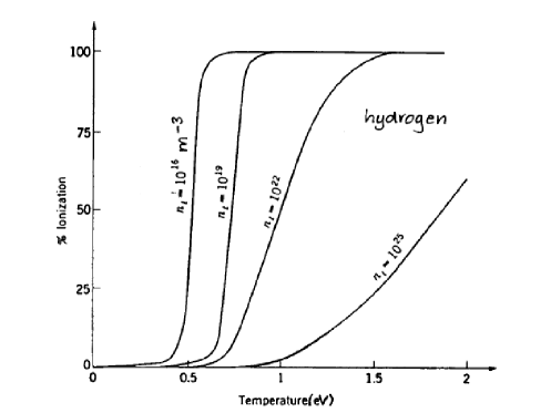
  Figure 1: Degree for Ionization for Hydrogen, with, I = 13.6 eV.

• Ionization can come from external medium (Ionosphere ? T = say 1000 K).

• Ionization can come from the proximity of atoms ? Share electrons : metal.

Classification

Say temperature $T$, density $N$.

Typical distance between two electrons: $N^{-1/3}$.

Typical Coulomb energy: $e^{2}/N^{-1/3}$.

Typical kinetic energy in classical regime: $k_{B}T$.

More kinetic energy than Coulomb: $k_{B}T>e^{2}/N^{-1/3}$. Big frontier.

Classical relativistic: $k_{B}T>mc^{2}$.

Then come quantum effects. When $T>$ Fermi temperature $T_{F}$, with $k_{B}T_{F}=\hbar^{2}(3\pi^{2}N)^{2/3}/2m_{e}$.

Thus, for $T<T_{F}$, energy increases with density, not temperature.

$k_{B}T_{F}<mc^{2}$, $k_{B}$ scales like $N^{2/3}$.

$k_{B}T_{F}>mc^{2}$, $k_{B}$ scales like $N^{1/3}$ (White Dwarfs to Neutron Stars?).

Important quantities

Time it takes to neutralize charge in-balance: Plasma frequency

$$\omega_{p}^{2}=\frac{4\pi Ne^{2}}{m_{e}}=9000\sqrt{N~{}[\mathrm{cm}^{-3}]}.$$ (2)

That’s why some waves bounce against the ionosphere.

Distance over which charge in-balance can exist: Debye length

$$\lambda_{D}=\frac{V_{th}}{\omega_{p}}=\sqrt{\frac{k_{B}T}{4\pi Ne}}=7.43~{}10^{2}\sqrt{T~{}[\mathrm{K}]/N~{}[\mathrm{cm}^{-3}]}~{}[\mathrm{cm}].$$ (3)

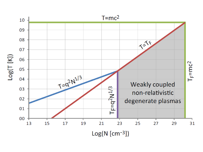
Figure 2: Classification of plasmas.

2 Kinetic theory

Vlasov and Boltzmann equations

Say only electrons + fixed positive background. Most basic description level. $G(\mathbf{r},\mathbf{p},t)d^{3}\mathbf{r}d^{3}\mathbf{p}$ = number of particles in $d^{3}\mathbf{r}d^{3}\mathbf{p}$ around $(\mathbf{r},\mathbf{p})$ at time $t$. How does it evolve?

Say a particle has momentum $\mathbf{p}$ at position $\mathbf{r}$, at time $t$. Say a force $\mathbf{F}$ acts on it. At time $t+dt$, it will have momentum $\mathbf{p}+\mathbf{F}dt$, and position $\mathbf{r}+\mathbf{p}/\gamma m~{}dt$ (non-quantum treatment).
Therefore, ALL particles in $d^{3}\mathbf{r}d^{3}\mathbf{p}$ around $(\mathbf{r},\mathbf{p})$ at time $t$ MUST be in $d^{3}\mathbf{r}d^{3}\mathbf{p}$ around $(r+\mathbf{p}/\gamma m~{}dt,\mathbf{p}+\mathbf{F}dt)$ at time $t+dt$. That means,

$$G\left(\mathbf{r}+\frac{\mathbf{p}}{\gamma m}dt,\mathbf{p}+\mathbf{F}dt,t+dt\right)=G(\mathbf{r},\mathbf{p},t)$$ (1)

The “hyper” volume element $d^{3}\mathbf{r}d^{3}\mathbf{p}$ does not change (Jacobian = 1 here). Just Taylor expand the left-hand-side to get the Vlasov Equation,

$$G(\mathbf{r},\mathbf{p},t)+\frac{\partial G}{\partial\mathbf{r}}\cdot\frac{\mathbf{p}}{\gamma m}dt+\frac{\partial G}{\partial\mathbf{p}}\cdot\mathbf{F}dt+\frac{\partial G}{\partial t}dt = G(\mathbf{r},\mathbf{p},t),$$

$$\Rightarrow\frac{\partial G}{\partial\mathbf{r}}\cdot\frac{\mathbf{p}}{\gamma m}+\frac{\partial G}{\partial\mathbf{p}}\cdot\mathbf{F}+\frac{\partial G}{\partial t} = 0.$$ (2)

Now, this result is NOT always right. Why?
We have assumed the force $\mathbf{F}$ does not change over $dt$. But $\mathbf{F}$ is an averaged force, in the same way the function $G$ is averaged (IGM = $10^{-6}$ part/cm^-3. If not averaged, $d^{3}\mathbf{r}$ must be gigantic, not infinitesimal). What if something “un-smooth” happened during $dt$ ?

Close collisions are local, quasi-instantaneous processes, sending some particles OUT of $d^{3}\mathbf{p}$ around $\mathbf{p}$, and some other particles INSIDE $d^{3}\mathbf{p}$ around $\mathbf{p}$, during $dt$. (Think about billiard ball collisions: local and instantaneous). We’ll then have,

$$G(\mathbf{r},\mathbf{p},t) + \frac{\partial G}{\partial\mathbf{r}}\cdot\frac{\mathbf{p}}{\gamma m}dt+\frac{\partial G}{\partial\mathbf{p}}\cdot\mathbf{F}dt+\frac{\partial G}{\partial t}dt$$ (3)

$$= G(\mathbf{r},\mathbf{p},t)+[\mathrm{Collisions}(\mathbf{r},t),~{}\mathbf{q}\rightarrow\mathbf{p},\forall\mathbf{q}]-[\mathrm{Collisions}(\mathbf{r},t),~{}\mathbf{p}\rightarrow\mathbf{q},\forall\mathbf{q}],$$

giving the Boltzmann Equation,

$$\frac{\partial G}{\partial\mathbf{r}}\cdot\frac{\mathbf{p}}{\gamma m}+\frac{\partial G}{\partial\mathbf{p}}\cdot\mathbf{F}+\frac{\partial G}{\partial t}=\int_{\mathbf{q}}[\mathrm{Collisions}(\mathbf{r},t),~{}\mathbf{q}\rightarrow\mathbf{p}]-[\mathrm{Collisions}(\mathbf{r},t),~{}\mathbf{p}\rightarrow\mathbf{q}].$$ (4)

The right-hand-side, referred to as the “collision term”, is analitically untractable. Yet, that’s the one driving the relaxation to a Maxwellian distribution $G_{M}\propto e^{-v^{2}}$. For practical purposes, alternative forms have been worked-out (Fokker-Planck/Landau, Balescu, Krook $\nu(G_{M}-G)$…).

Vlasov or Boltzmann ?

In a plasma, particles are influenced by,

• Close collisions, changing $\mathbf{p}$ rapidly and appreciably (say $\theta>\pi/2$). Accounted for by the collision term in the kinetic equation.

• “Distant” collisions, which amount to the influence of the overall plasma ($\rho,\mathbf{J}\rightarrow\mathbf{E},\mathbf{B}$). Accounted for by the Force term in the kinetic equation.

Define a “close” collision by closest approach $<R_{L}$, such as $e^{2}/R_{L}=E_{K}$ where $E_{K}$ is the typical Kinetic energy ($k_{B}T$ or $k_{B}T_{F}$). Frequency for such collisions is roughly $\nu\sim nR_{L}^{2}v_{K}$, with $mv_{K}^{2}=E_{K}$. Time scale for “distant” collisions if $\sim\omega_{p}^{-1}$. Vlasov’s equation, with collision term = 0, is valid for $\nu\ll\omega_{p}$, i.e.,

$$n\left(\frac{e^{2}}{E_{K}}\right)^{2}\sqrt{\frac{E_{K}}{m}}\ll\sqrt{\frac{4\pi ne^{2}}{m}}\Leftrightarrow e^{2}n^{1/3}\ll E_{K},$$ (5)

which just defines weakly coupled plasmas, where there is more kinetic energy than Coulomb potential energy, whether degenerate or not.

The Vlasov-Maxwell system

For weakly coupled plasmas, the first equation needed is therefore Vlasov’s with F = Lorentz,

$$\frac{\partial G}{\partial t}+\frac{\mathbf{p}}{\gamma m}\cdot\frac{\partial G}{\partial\mathbf{r}}+q\left[\mathbf{E}(\mathbf{r},t)+\frac{\mathbf{v}}{c}\times\mathbf{B}(\mathbf{r},t)\right]\cdot\frac{\partial G}{\partial\mathbf{p}}=0.$$ (6)

System is closed with Maxwell’s equations, where charge and current densities are given by,

$$\rho(\mathbf{r},t) = \int G(\mathbf{r},\mathbf{p},t)d^{3}\mathbf{p},$$

$$\mathbf{J}(\mathbf{r},t) = \int qG(\mathbf{r},\mathbf{p},t)\mathbf{v}d^{3}\mathbf{p}.$$ (7)

Eqs. (6,The Vlasov-Maxwell system), together with Maxwell’s, form the Vlasov-Maxwell closed system of equations. In 1D along axis $x$, we just have for $G(x,p,t)$ and $E(x,t)$,

$$\frac{\partial G}{\partial t}+\frac{p}{\gamma m}\frac{\partial G}{\partial x}+qE\frac{\partial G}{\partial p}=0,~{}~{}~{}~{}~{}\frac{\partial E}{\partial x}=4\pi q\int G(x,p,t)dp,$$ (8)

with $q=-e$ for electrons. Landau damping comes from these 2, originally with $\gamma=1$.

3 From Kinetic to Fluid to MHD Equations

From Kinetic to Fluid

Fluid equations can be deduced from the moments of the kinetic equation. The fluid macroscopic density $n$, velocity $\mathbf{v}$ and pressure tensor $\mathbf{P}$ are defined through,

$$n(\mathbf{r},t) = \int F(\mathbf{r},\mathbf{u},t)d^{3}\mathbf{u},~{}~{}~{}~{}\mathbf{P}(\mathbf{r},t)=\int m(\mathbf{u}-\mathbf{v})\otimes(\mathbf{u}-\mathbf{v})F(\mathbf{r},\mathbf{u},t)d^{3}\mathbf{u},$$

$$n(\mathbf{r},t)\mathbf{v}(\mathbf{r},t) = \int\mathbf{u}F(\mathbf{r},\mathbf{u},t)d^{3}\mathbf{u},~{}~{}$$ (1)

where $\otimes$ is “dyadic” product $\mathbf{u}\otimes\mathbf{v}=(u_{i}v_{j})$. If our plasma is cold, which kinetically means $F(\mathbf{r},\mathbf{u},t)=\delta[\mathbf{u}-\mathbf{v}(\mathbf{r},t)]G(\mathbf{r},t)$, the density $n(\mathbf{r},t)$ and the velocity $\mathbf{v}(\mathbf{r},t)$ are what we would expect. Interestingly enough, the pressure tensor vanishes. Microsopic velocity spread translates to macroscopic pressure. Consider now the non-relativistic Vlasov kinetic equation,

$$\frac{\partial F}{\partial t}+\mathbf{v}\cdot\frac{\partial F}{\partial\mathbf{r}}+\frac{\mathbf{E}+\mathbf{v}\times\mathbf{B}/c}{m}\cdot\frac{\partial F}{\partial\mathbf{v}}=0.$$ (2)

The moments of the equation give,

$$\int[\mathrm{Vlasov}]~{}~{}d^{3}\mathbf{p} \Rightarrow \frac{\partial n}{\partial t}+\frac{\partial}{\partial\mathbf{r}}\cdot(n\mathbf{v})=0,$$

$$\int m\mathbf{u}~{}[\mathrm{Vlasov}]~{}~{}d^{3}\mathbf{p} \Rightarrow mn\left(\frac{\partial\mathbf{v}}{\partial t}+\mathbf{v}\cdot\frac{\partial\mathbf{v}}{\partial\mathbf{r}}\right)=qn\left(\mathbf{E}+\frac{\mathbf{v}}{c}\times\mathbf{B}\right)-\frac{\partial}{\partial\mathbf{r}}\cdot\mathbf{P}.$$ (3)

For isotropic pressure with $\mathbf{P}=p\mathbf{I}$, the last term is just the usual gradient $\partial p/\partial\mathbf{r}=\nabla p$.
The “convective derivative” term $(\partial_{t}+\mathbf{v}\cdot\nabla)$ simply follows a fluid element.

At this stage, you can close the system introducing a relation between $n(\mathbf{r},t)$ and $p(\mathbf{r},t)$, that is, an equation of state. Like for the first moment and the pressure, the Vlasov moment $\int u^{n}(~{})d^{3}u$ always yields a macroscopic quantity $\propto\int u^{n+1}(~{})d^{3}u$ from the $\mathbf{v}\cdot\partial F/\partial\mathbf{r}$ term.
Still regarding the micro/macro duality: a non-zero collision term in the Vlasov equation is needed to recover viscosity or friction on the macro level.

From Fluid to MHD

We have initially one distribution function $F_{i}(\mathbf{r},\mathbf{u},t)$ per species. The procedure above shows we eventually have one set of fluid equations per species. Assume we just have protons and electrons of densities $n_{p}(\mathbf{r},t)$ and $n_{e}(\mathbf{r},t)$. If we want to describe fast phenomenon where electrons could be decoupled from protons (faster than $\omega_{p}^{-1}$, or smaller than $\lambda_{D}$), we need to keep two sets of equations. The so-called Braginskii Equations might be the most elaborate version of this option.

What if we’re interested in slow $\tau\ll\omega_{p}^{-1}$, and large scale $\gg\lambda_{D}$, effects? Electrons are expected to closely follow protons. The plasma is a electron/proton “soup”. Electroneutrality on these scales gives $n_{p}(\mathbf{r},t)\sim n_{e}(\mathbf{r},t)$. In the same way we defined the fluid quantities (From Kinetic to Fluid) and found they obey Eqs. (From Kinetic to Fluid), we define the MHD variables,

$$\rho(\mathbf{r},t) = m_{p}n_{p}(\mathbf{r},t)+m_{e}n_{e}(\mathbf{r},t),~{}~{}~{}~{}~{}~{}\mathbf{V}(\mathbf{r},t)=\frac{m_{e}\mathbf{v_{e}}+m_{p}\mathbf{v_{p}}}{m_{e}+m_{p}}$$

$$\mathbf{J}(\mathbf{r},t) = qn_{p}(\mathbf{r},t)\mathbf{v}_{p}(\mathbf{r},t)-qn_{e}(\mathbf{r},t)\mathbf{v}_{e}(\mathbf{r},t).$$ (4)

Combining the fluid equations for electrons and protons yields,

$$\frac{\partial\rho}{\partial t}+\frac{\partial(\rho\mathbf{V})}{\partial\mathbf{r}} = 0,$$ (5)

$$\rho\left(\frac{\partial\mathbf{V}}{\partial t}+\mathbf{V}\cdot\frac{\partial\mathbf{V}}{\partial\mathbf{r}}\right) = \frac{\mathbf{J}}{c}\times\mathbf{B}-\nabla(\overbrace{p_{i}+p_{e}}^{P})+\rho\mathbf{g},$$ (6)

where $\rho\mathbf{E}$ is neglected with respect to the Lorentz force, as $n_{e}\sim n_{p}\Rightarrow\mathbf{E}\sim 0$. Also, a gravity term $\rho\mathbf{g}$ is added here. Its fluid counterpart in Eq. (From Kinetic to Fluid) would obviously be $nm\mathbf{g}$. The system is closed through,

$$\frac{\partial\mathbf{B}}{\partial t}=-c\nabla\times\mathbf{E},~{}~{}~{}~{}~{}\nabla\times\mathbf{B}=\frac{4\pi}{c}\mathbf{J}+\cancel{\frac{1}{c}\frac{\partial\mathbf{E}}{\partial t}}.$$ (7)

Inserting $\mathbf{J}=c\nabla\times\mathbf{B}/4\pi$ into Eq. (6) gives the usual magnetic pressure and tension terms. The last equation used to close the system is Ohm’s law, which simplest version reads

$$\mathbf{J}=\sigma\left(\mathbf{E}+\frac{\mathbf{V}}{c}\times\mathbf{B}\right),$$ (8)

where $\sigma$ is the medium conductivity. This equation is just $\mathbf{J}=\sigma\mathbf{E}$ in the fluid-frame at velocity $\mathbf{V}$, transformed in the Lab. frame. Ideal MHD sets $\sigma=\infty$, so that $\mathbf{E}=-\mathbf{V}\times\mathbf{B}/c$. Two concluding remarks:

• Yes, we sometime consider $\mathbf{E}=0$, like in Eqs. (6) and (7-right), and sometime $\mathbf{E}\neq 0$ like in Ohm’s law or (7-left). Kulsrud explains well how this proves reasonable.

• We’ve cheated a little bit. We use the collisionless Vlasov’s equation, and then talk about EOS or Ohm’s law, which imply collisions. It’s just far simpler to forget about collisions at the kinetic/micro level, derive the fluid equations, and then get collisions back into the game, kind of empirically, at the fluid/macro level.

4 Linear Landau damping - The Maths

Just a piece of a vast problem: Energy exchange between waves and particles in a plasma. Simply put, in terms of the energy transfer direction:

• Waves $\rightarrow$ Particles: Particle acceleration, wave damping.

• Particles $\rightarrow$ Waves: Wave instability.

The original paper is Ref. [1]. Landau damping is one of the most studied/debated problem in plasma physics. Nice Maths and Physical derivation.

Calculation overview

Since the calculation is quite subtle and long, it may be useful to get a general overview from the very beginning. Here are the steps we will follow:

1. Derivation of the dispersion equation $\epsilon(k,\omega)=0$ from the 1D Vlasov-Poisson system.

2. Landau contour, the continuity requirement and the Laplace transform.

3. Resolution for small damping and any distribution function.

4. Maxwellian distribution.

Dispersion Equation

Start from 1D non-relativistic equations for $F(x,v=p/m,t)$ and field $E(x,t)$,

$$0 = \frac{\partial F}{\partial t}+v\frac{\partial F}{\partial x}-e\frac{E}{m}\frac{\partial F}{\partial v},$$ (1)

$$\frac{\partial E}{\partial x} = 4\pi e\left[n_{0}-\int F(x,v,t)dv\right],$$ (2)

where $n_{0}=\int F_{0}dv$ is the equilibrium density. Assume $F=F_{0}+F_{1}$, with $\mid F_{1}\mid\ll\mid F_{0}\mid$, $F_{0}$ being an equilibrium solution. Same for $E$. The equilibrium electric field $E_{0}=0$. Linearizing Eqs. (1,2), assuming $F_{1},E_{1}\propto\exp(ikx-i\omega t)$, gives

$$0 = -i\omega F_{1}+ikvF_{1}-e\frac{E_{1}}{m}\frac{\partial F_{0}}{\partial v},$$ (3)

$$ikE_{1} = -4\pi e\int F_{1}(x,v,t)dv.$$ (4)

Extract $F_{1}$ from the first equation, and plug it into the second,

$$\epsilon(k,\omega) = 0,~{}~{}~{}\mathrm{with},$$

$$\epsilon(k,\omega) = 1-\frac{\omega_{p}^{2}}{k^{2}}\int\frac{f_{0}^{\prime}}{v-\omega/k}dv,$$ (5)

where $\omega_{p}^{2}=4\pi n_{0}e^{2}/m$, $f_{0}=F_{0}/n_{0}$ and $f_{0}^{\prime}=\partial f_{0}/\partial v$. This dispersion relation was first obtained by Vlasov in 1925 [2]. It shows $\omega$ should be imaginary. Otherwise, we have a problem, unless $f_{0}^{\prime}(\omega/k)=0$. The dielectric function $\epsilon(k,\omega)$ has therefore a real and an imaginary part, which for all kind of systems, is related to dissipation.

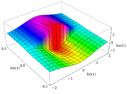
Figure 3: Imaginary part of $G=\int e^{-u^{2}}du/u-x$, for $x\in\mathbb{C}$. The real axis is a discontinuity.

We could just consider $\omega$ imaginary and take this quadrature as it is, integrating along the real axis. But there’s a problem. The resulting function of $\omega$ is discontinuous, precisely when crossing the real axis. As an illustration, Fig. 3 displays the imaginary part of $G=\int e^{-u^{2}}du/u-x$, for $x\in\mathbb{C}$. The discontinuity is obvious around $\mathrm{Im}(x)=0$. One part of the plan has to be physically meaningful, and the other not. But which one? We could try both options, and check that damping comes only when choosing the upper one. But what if we didn’t know in the first place that a Maxwellian is stable? We shall see that a Laplace analysis of the problem can fully answer the question, and will indeed tell us that the “physical” half-plane is the upper one.

Admitting for now the upper-plane is the physical one, what do we do with the lower one? The answer is that we have to “analytically continuate” the function we have on the upper-plane, to the lower one. This means finding a function on the lower plane which makes a continuous, “analytical” junction, with what we have on the upper one. In this respect, a uniqueness theorem from complex analysis helps: if somehow we find an expression in the lower plane matching what we have in the upper one, then this is the only one. The Landau contour is going to do all of that for us: providing a contour of integration equivalent to an integration over the real axis for $\mathrm{Im}(\omega)>0$, and an analytical continuation of the later in the lower plane $\mathrm{Im}(\omega)<0$.

Landau contour, the continuity requirement and the Laplace transform

Let’s first give the solution found by Landau, namely the famous “Landau contour”. Figure 4 shows this integration contour has 3 very distinctive features:

1. The Landau contour is not closed by the “usual” semi-circle in the lower or upper half-plane.

2. The pole $\omega/k=(\omega_{r}+i\delta)/k$ must always lie on the same side of the Landau contour.

3. So, which side? The Landau contour goes below the pole.

These contour prescriptions are called the “Landau prescriptions”, and the corresponding contour, the “Landau contour”. We thus rewrite from now on Eq. (5) as

$$\epsilon(k,\omega)=1-\frac{\omega_{p}^{2}}{k^{2}}\int_{L}\frac{f_{0}^{\prime}}{v-\omega/k}dv,$$ (6)

where $\int_{L}$ means integration along the Landau contour. Let’s now find out about these 3 features.

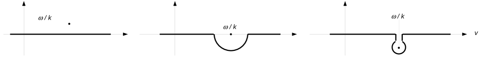
Figure 4: The Landau integration contour. It is not closed. It lies always on the same side of the pole. It lies below the pole.

The contour is not closed

The contour just goes from $v=-\infty$ to $+\infty$, and is not closed in the upper or lower half-plane, as “usual”, because we have no guarantee $f_{0}^{\prime}(v)$ behaves correctly there, so as to cancel the integration on the semi-circle at infinite radius. Indeed, considering a Maxwellian with $f_{0}^{\prime}\propto e^{-v^{2}}$ and setting $v=R_{v}e^{i\theta_{v}}$ to parameterize the integration on a circle of radius $R_{v}$, we find $f_{0}^{\prime}\propto e^{-R_{v}^{2}\cos 2\theta_{v}}$ which can hardly be considered a vanishing quantity at $R_{v}\rightarrow\infty$ for any $\theta_{v}\in[0,\pi]$ (or $[0,-\pi]$, if you close in the lower half-plane).

Always on the same side

Assume $\omega=\omega_{r}+i\delta$, with $\delta>0$. As long as $\delta$ remains positive in Eq. (5), the calculation does not pose any conceptual problem as the pole is not on the real axis, and continuity is guaranteed.

Now, what if $\delta$ approaches 0, and the pole $\omega/k$ even gets to cross the real axis? We would like $\epsilon(k,\omega)$ to be a continuous function of $\omega$. Assume first we leave the integration contour unchanged (the real axis for $v$), and compare the quadrature for $\omega=\omega_{r}+i\delta$ and $\omega=\omega_{r}-i\delta$. The influence of the pole is mostly felt where the denominator is minimum at $v\sim\omega_{r}/k$, so let’s locally get $f_{0}^{\prime}$ out of the integral and compare,

$$I_{1}=\int\frac{dv}{v-(\omega_{r}+i\delta)/k}~{}~{}~{}~{}\mathrm{and}~{}~{}~{}~{}I_{2}=\int\frac{dv}{v-(\omega_{r}-i\delta)/k}.$$ (7)

The difference $I_{1}-I_{2}$ is,

$$I_{1}-I_{2}=2i\int\frac{\delta/k}{(v-\omega_{r}/k)^{2}+(\delta/k)^{2}}dv.$$ (8)

The continuity of $\epsilon(k,\omega)$ demands the expression above vanishes when $\delta\rightarrow 0^{+}$. The problem is that it does not. Instead, the quadrature tends to $\pi$ (see function $G_{2}$ in Appendix A), so that we indeed have a jump of amplitude $2i\pi$ when crossing the real axis.

The only way to avoid this is to deform the integration contour in such a way that it always lies on the same side of the pole $\omega/k$.

The contour goes below the pole

To understand why the contour goes below the pole and not above like in Fig. 6, we need to follow Landau in rethinking the problem in terms of the time evolution of a perturbation applied at $t=0$. The Fourier technique is not well suited for that because it entails an integration from $t=-\infty$ to $+\infty$. By design, it does not single out any special moment in between. By contrast, the Laplace transform involves times only from zero to $+\infty$. As shall be checked, the Laplace transform technique gives an unambiguous response about the location of the pole with respect to the integration contour.

Considering a function $h(t)$, its Laplace transform $\widehat{h}(\omega)$ and the inversion formula, read

$$\widehat{h}(\omega) = \int_{0}^{\infty}e^{i\omega t}h(t)dt,$$ (10)

$$h(t) = \int_{C_{L}}e^{-i\omega t}\widehat{h}(\omega)d\omega,$$ (11)

where the contour $C_{L}$ pictured on Fig. 5, passes above all the poles of $\widehat{h}(\omega)$ at height $\sigma>0$, and can be closed in the lower half-plane where $e^{-i\omega t}$ behaves conveniently as to cancel the integral at infinity there. Note that although the requirement $\sigma>0$ is emphasized in the book (p. 139), I still have to understand why being above all the poles is not enough. And as we shall see very soon, $\sigma>0$ is the key to the choice of the right part of the $\omega$ complex plane.

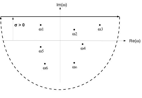
Figure 5: Laplace integration contour. Goes from $\omega=-\infty+i\sigma$ to $+\infty+i\sigma$ with $\sigma>0$, and is closed in the lower half-plane. By design, $\sigma>0$ and such that every single poles $\omega_{1},\ldots,\omega_{n}$ of the integrand lie inside the contour.

Let’s compute from the Maxwell-Vlasov Eqs. (1,2) the time evolution of the system considering,

$$F(x,v,t) = n_{0}f_{0}(v)+F_{1}(v,t)e^{ikx},$$ (12)

$$E(x,t) = E_{1}(t)e^{ikx},$$ (13)

assuming $F_{1},E_{1}$ are first order quantities, and $F_{1}(v,t=0)e^{ikx}$ is the perturbation initially applied. The linearized Vlasov equation reads,

$$\frac{\partial F_{1}(v,t)}{\partial t}+ikvF_{1}(v,t)-\frac{en_{0}}{m}E_{1}(t)f_{0}^{\prime}(v)=0.$$ (14)

If we multiply by $e^{i\omega t}$ and take the integral from $t=0$ to $+\infty$, an integration by part on the time derivative term gives,

$$\int_{0}^{\infty}e^{i\omega t}\frac{\partial F_{1}(v,t)}{\partial t}dt = \left[e^{i\omega t}F_{1}(v,t)\right]_{0}^{\infty}-i\omega\int_{0}^{\infty}e^{i\omega t}F_{1}(v,t)dt$$ (15)

$$= -F_{1}(v,0)-i\omega\widehat{F}_{1}(v,\omega),$$

where $\lim_{t\rightarrow\infty}e^{i\omega t}F_{1}(v,t)=0$ has been assumed. On the one hand, the very existence of the Laplace transform of $F_{1}(v,\omega)=\int F_{1}(v,t)e^{i\omega t}dt$ implies it. On the other hand, a important conclusion of the paper is that for large times, $F_{1}(v,t)\propto e^{ikvt}$ (see [1] p. 452, and Plasma Talk 5). This point is discussed neither in the book, nor in the original paper. Using Eqs. (15,14) then gives,

$$(ikv-i\omega)\widehat{F}_{1}(v,\omega)-\frac{en_{0}}{m}\widehat{E}_{1}(\omega)f_{0}^{\prime}(v)=F_{1}(v,0),$$ (16)

where $F_{1}(v,0)$ now acts like a “source term” at the right-hand-side. A few more manipulations exploiting Poisson’s equation (2) give,

$$\widehat{E}_{1}(\omega)=\frac{1}{\epsilon(k,\omega)}\frac{4\pi e}{k^{2}}\int_{-\infty}^{\infty}\frac{F_{1}(v,0)dv}{v-\omega/k},$$ (17)

where $\epsilon(k,\omega)$ is identical to Eq. (5). The time dependant electric field given by the inversion formula (11) is,

$$E_{1}(t)=\int_{C_{L}}e^{-i\omega t}\widehat{E}_{1}(\omega)d\omega=\int_{C_{L}}\frac{e^{-i\omega t}}{\epsilon(k,\omega)}\left[\frac{4\pi e}{k^{2}}\int_{-\infty}^{\infty}\frac{F_{1}(v,0)dv}{v-\omega/k}\right]d\omega.$$ (18)

In contradistinction with Eq. (5) where the contour issue is puzzling, the Laplace technique used here is clear: The $v$-integration in $\epsilon(k,\omega)$ does go along the real axis, and the $\omega$-integration is performed at fixed $\mathrm{Im}(\omega)=\sigma>0$. It means that in Eq. (18), which computes a physical quantity, the dielectric function $\epsilon(k,\omega)$ is calculated with $\omega$ above the real $v$-axis.

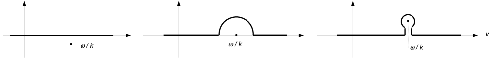
Figure 6: Forbidden option for the contour. Continuity is preserved, but the contour lies above the pole, in contradiction with the Laplace prescription.

That answers the question we had: the physically meaningful half-plane we were wondering about after Eq. (5) is the upper one. The kind of contour pictured on Fig. 6 is thus “forbidden”.

Incidentally, what are the poles of the integrand in Eq. (18)? For “normal”, smooth initial excitations $F_{1}(v,0)$, the term between brackets won’t have poles, so that our poles $\omega_{1},\ldots,\omega_{n}$ are eventually the zeros of $\epsilon(k,\omega)$. The $\omega$-integration of Eq. (18) on the closed contour $C_{L}$ will thus give, with $\omega_{j}=\omega_{r,j}+i\delta_{i}$,

$$E_{1}(t)=2i\pi\sum_{j=1}^{n}Res(j)\equiv\sum_{j=1}^{n}A_{j}\exp(-i\omega_{j}t)=\sum_{j=1}^{n}A_{j}\exp(-i\omega_{r,j}t)e^{\delta_{j}t},$$ (19)

which for large times will be governed by the largest $\delta_{j}$. Therefore, the Laplace transform approach cannot spare us the resolution of $\epsilon(k,\omega)=0$, as these zeros are the building blocks of the temporal response of the system.

Resolution for small damping

We suppose small damping, that is $|\delta|\ll|\omega_{r}|$, and Taylor expand Eq. (6),

$$\epsilon(k,\omega_{r}+i\delta) = \epsilon_{r}(k,\omega_{r})+i\delta\left.\frac{\partial\epsilon_{r}}{\partial\omega_{r}}\right|_{\delta=0}+i\left[\epsilon_{i}(k,\omega_{r})+i\delta\left.\frac{\partial\epsilon_{i}}{\partial\omega_{r}}\right|_{\delta=0}\right]$$ (20)

$$= \epsilon_{r}(k,\omega_{r})+i\epsilon_{i}(k,\omega_{r})+\delta\left[i\frac{\partial\epsilon_{r}}{\partial\omega_{r}}-\frac{\partial\epsilon_{i}}{\partial\omega_{r}}\right]_{\delta=0}$$

$$= \epsilon(k,\omega_{r})+i\delta\left.\frac{\partial\epsilon_{r}}{\partial\omega_{r}}\right|_{\delta=0}+o(\delta),$$

where the $o(\delta)$ (negligible with respect to $\delta$), comes from the fact that $\epsilon_{i}(\delta=0)=0$ (no damping, no dissipation, no imaginary dielectric function).

The first term $\epsilon(k,\omega_{r})$ is given by Eq. (6) setting $\omega=\omega_{r}$, or taking the limit of $\epsilon(k,\omega_{r}+i\delta)$ for $\delta\rightarrow 0^{+}$. The part of the integration along the real axis for $v\in[-\infty,\omega_{r}/k-\varepsilon]\cup[\omega_{r}/k+\varepsilon,+\infty]$ gives the so-called “Cauchy Principal Part”, denoted P here. The part corresponding to the semi-circle (see Fig. 4 middle) gives the semi-residue for $v=\omega_{r}/k$. An alternative way of deriving this result, considering the limit $\delta\rightarrow 0^{+}$, is reported in Appendix A. We thus get,

$$\epsilon(k,\omega_{r})=1-\frac{\omega_{p}^{2}}{k^{2}}\left[\mathbf{P}\int\frac{f_{0}^{\prime}}{v-\omega_{r}/k}dv+i\pi f_{0}^{\prime}(\omega_{r}/k)\right].$$ (21)

This result allows to compute $\partial\epsilon_{r}/\partial\omega_{r}$ in Eq. (20), which eventually gives,

$$\epsilon(k,\omega)=1-\frac{\omega_{p}^{2}}{k^{2}}\mathbf{P}\int\frac{f_{0}^{\prime}}{v-\omega_{r}/k}dv-i\frac{\omega_{p}^{2}}{k^{2}}\left[\pi f_{0}^{\prime}(\omega_{r}/k)+\delta\frac{\partial}{\partial\omega_{r}}\mathbf{P}\int\frac{f_{0}^{\prime}}{v-\omega_{r}/k}dv\right].$$ (22)

Equating the real part to zero yields,

$$\frac{\omega_{p}^{2}}{k^{2}}\mathbf{P}\int\frac{f_{0}^{\prime}}{v-\omega_{r}/k}dv=1,$$ (23)

which was the result obtained by Vlasov in the first place. Canceling the imaginary part gives directly the damping rate,

$$\delta=-\pi\frac{f_{0}^{\prime}(\omega_{r}/k)}{\frac{\partial}{\partial\omega_{r}}\mathbf{P}\int\frac{f_{0}^{\prime}}{v-\omega_{r}/k}dv}.$$ (24)

Eqs. (23, 24) formally solve the problem in terms of the distribution function. A first order evaluation of P$\sim k^{2}/\omega_{r}^{2}$ (see Eq. (27) below), gives

$$\omega_{r} = \omega_{p},~{}~{}~{}~{}\mathrm{and}~{}\mathrm{then}$$ (25)

$$\frac{\delta}{\omega_{p}} = \frac{\pi}{2}\frac{\omega_{p}^{2}}{k^{2}}f_{0}^{\prime}(\omega_{p}/k).$$

The rate $\delta$ has the sign of $f_{0}^{\prime}(\omega_{p}/k)$. That means that if $f_{0}$ decreases for $v=\omega_{p}/k$, the waves is damped because $\delta<0$. But if $f_{0}$ increases for $v=\omega_{p}/k$, we have $\delta>0$ and the wave can actually grow.

One could argue we started initially assuming $\delta$ positive, and find it can be negative here. It is not a problem for the following reason: Eq. (22) we found assuming $\delta>0$ is continuous at $\delta=0$. It must therefore be identical to the integration on the Landau contour on both sides of the real axis. We can therefore confidently solve it regardless of the sign of $\delta$. In other words, thanks to the Landau contour, we can compute the result as if $\delta$ was positive, and then don’t care about the sign.

Historically, Vlasov first ran into Eq. (5). He escaped the problem posed by the pole on the real axis by considering only the P of the quadrature. He did so apparently without much foundation, which Landau denounced without mercy in [1]. We understand from the analysis above that doing so, he missed the imaginary part which would have led to the “Vlasov damping”.

Maxwellian distribution

Let’s finally consider a 1D Maxwellian distribution,

$$f_{0}(v)=\frac{1}{\sqrt{2\pi k_{B}T/m}}e^{-mv^{2}/2k_{B}T}.$$ (26)

For phase velocities $\omega_{r}/k$ much larger than the thermal velocity $V_{th}=\sqrt{k_{B}T/m}$, we can expand the denominator in powers of $kv/\omega_{r}$, since that quantity is small where the numerator is relevant. We thus have,

$$\mathbf{P}\int\frac{f_{0}^{\prime}}{v-\omega_{r}/k}dv = -\frac{k}{\omega_{r}}\int f_{0}^{\prime}\left(1+\frac{kv}{\omega_{r}}+\frac{k^{2}v^{2}}{\omega_{r}^{2}}+\frac{k^{3}v^{3}}{\omega_{r}^{3}}+\cdots\right)dv$$ (27)

$$= \frac{k^{2}}{\omega_{r}^{2}}+3\frac{k_{B}T}{m}\frac{k^{4}}{\omega_{r}^{4}}+\cdots$$

For small $k$, namely $kV_{th}/\omega_{r}\sim kV_{th}/\omega_{p}\ll 1$, Eq. (23) now gives,

$$\omega_{r}^{2}=\omega_{p}^{2}(1+3k^{2}\lambda_{D}^{2}),~{}~{}~{}\mathrm{with}~{}~{}~{}\lambda_{D}=\frac{\sqrt{k_{B}T/m}}{\omega_{p}}.$$ (28)

We finally (phew!) use Eq. (24) to extract the damping rate. On the one hand, we compute the derivative of the P with respect to $\omega_{r}$ using Eq. (27), and then simply set $\omega_{r}=\omega_{p}$ in the result. On the other hand, we set $\omega_{r}=\omega_{p}$ in $f_{0}^{\prime}$ to find

$$\delta=-\omega_{p}\frac{\sqrt{\pi/8}}{k^{3}\lambda_{D}^{3}}\exp\left(-\frac{1}{2k^{2}\lambda_{D}^{2}}\right).$$ (29)

Fluid theory just gives the real part of the frequency, namely Eq. (28), so that Landau damping is a purely kinetic effect.

Appendix A

Let’s derive,

$$\int_{L}\frac{f_{0}^{\prime}}{v-\omega_{r}/k}dv=\mathbf{P}\int\frac{f_{0}^{\prime}}{v-\omega_{r}/k}dv+i\pi f_{0}^{\prime}(\omega_{r}/k),$$ (30)

used for Eq. (21), without using the residue theorem. For $\omega=\omega_{r}+i\delta$ with $\delta>0$, integration along the Landau contour is equivalent to an integration along the real axis. Let’s thus assume $\delta>0$ and compute,

$$I=\lim_{\delta\rightarrow 0^{+}}\int_{-\infty}^{\infty}\frac{f_{0}^{\prime}}{v-(\omega_{r}+i\delta)/k}dv.$$ (31)

We multiply the numerator and the denominator of the integrand by $(v-\omega_{r}/k)+i\delta/k$, which is the complex conjugate of the denominator. We get an expression with a purely real, non singular denominator, and clearly separated real and imaginary parts,

$$I=\lim_{\delta\rightarrow 0^{+}}\int_{-\infty}^{\infty}\underbrace{\frac{(v-\omega_{r}/k)^{2}}{(v-\omega_{r}/k)^{2}+(\delta/k)^{2}}}_{G_{1}}\frac{f_{0}^{\prime}}{(v-\omega_{r}/k)}dv+i\int_{-\infty}^{\infty}\underbrace{\frac{\delta/k}{(v-\omega_{r}/k)^{2}+(\delta/k)^{2}}}_{G_{2}}f_{0}^{\prime}dv.$$ (32)

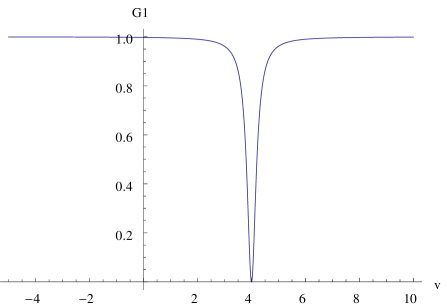
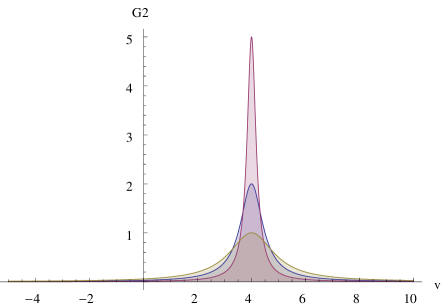
Figure 7: Functions $G_{1}$ and $G_{1}$ involved in Eq. (32). For small $\delta/k$, $G_{1}$ is almost 1 everywhere, except for $v=\omega_{r}/k$, where it is 0. $G_{2}$ peaks at $v=\omega_{r}/k$ and tends to 0 elsewhere, while its integral is always $\pi$, like a Dirac $\delta$ function. Parameters are $\omega_{r}/k=4$, $\delta/k=0.2$ for $G_{1}$, and $\delta/k=0.2,0.5,1$ for $G_{2}$.

Regarding the real part, the factor $G_{1}$ of the integrand is 0 for $v=\omega_{r}/k$, and $\sim 1$ for $\delta/k\ll|v-\omega_{r}/k|$. It tends to the P$\int f_{0}^{\prime}/(v-\omega_{r}/k)$ for small $\delta/k$ (see Fig. 7). The factor $G_{2}$ of the integrand of the imaginary part departs from 0 only for $v\sim\omega_{r}/k$. But its integral is always $\pi$. For small $\delta/k$, the quadrature thus tends to $\pi f_{0}^{\prime}(\omega_{r}/k)$, and we are back to (30).

This calculation is consistent with the Landau contour integration only for $\delta\rightarrow 0^{+}$. This is because in such case, the real axis along which we perform the integration (32) coincide with the Laundau contour. If we were to compute Eq. (32) for $\delta\rightarrow 0^{-}$, we would find the opposite imaginary part, just because in this case, the real axis no longer fits the Landau contour. The latter, instead, is deformed and keeps passing below the pole, precisely to avoid the discontinuity.

5 Landau damping - The Physics, Plasma Echo, and a (little) word about the non-linear problem

While the original paper [1] is purely mathematical, a clearer physical picture is provided in Landau’s book ([2], §30 p. 126). Suppose we switch on at $t=0$ a 1D electrostatic wave $\mathbf{E}=E_{0}\sin(kx-\omega t)\mathbf{x}$, traveling at $v_{\phi}=\omega/k$ along with a particle with velocity $v_{0}$ at $t=0$. For $v_{0}$ slightly larger than $v_{\phi}$, the particle is trapped in the wave potential, where it is going to oscillate. Doing so, it ends up with an average velocity close to the wave velocity $v_{\phi}$. It should thus loose energy, and the energy goes to the wave. Situation is reversed for particles initially slightly slower than the wave. They end up gaining energy from the wave.

If slower particles are more numerous than the faster ones, the wave looses more than it gains, which means it is damped. Let’s now “Fermi-calculate” this, not following Fermi but Jackson [3] and Spitzer [4] (who follows Jackson). Landau uses a slightly different approach, still implying a calculation with some small parameter eventually tending to zero. I chose Jackson precisely because there’s no such trick in his strategy. The reasoning is non-relativistic.

To start with, which particles can enter the game? If their velocity is too high relatively to the wave, they will flow from one potential crest to another, without much net energy exchange. The ones for which energy exchange is possible, are the ones which will be trapped by the potential. The wave potential height is,

$$\Delta\varphi=\frac{qE_{0}}{k}.$$ (1)

The maximum particle velocity $\Delta v$ in the wave-frame at $v_{\phi}$ must then satisfy,

$$\frac{1}{2}m(\Delta v)^{2}=\Delta\varphi~{}~{}\Rightarrow~{}~{}(\Delta v)^{2}=\frac{2qE_{0}}{mk}.$$ (2)

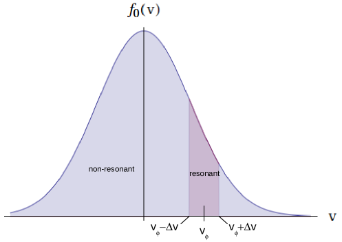
Figure 8: Division of the plasma between non-resonant and resonant (trapped) particles. Only resonant particles contribute to the calculation. After [5].

Thus, only particles with velocity $v\in[v_{\phi}-\Delta v,v_{\phi}+\Delta v]$ in the lab-frame can be caught by the wave. This is pictured on Fig. 8, taken from another great work on Landau damping by Dawson [5]. For a particle near the center of this interval, we take $\sin x\sim x$ for the field, and the equation of motion in the wave-frame reads

$$m\frac{d^{2}x}{dt^{2}}+qE_{0}kx=0~{}~{}\Rightarrow~{}~{}\frac{d^{2}x}{dt^{2}}+\omega_{osc}^{2}~{}x=0,~{}~{}\mathrm{where}~{}~{}\omega_{osc}^{2}=\frac{qE_{0}k}{m},$$ (3)

showing it oscillates in the wave potential with frequency $\omega_{osc}$.

Before it was trapped, the particle energy in the lab-frame was just $W_{1}=mv^{2}/2$. After the trapping, the energy is

$$W_{2}=\frac{1}{2}m\left(v_{\phi}^{2}+(v-v_{\phi})^{2}\right),$$ (4)

where $\frac{1}{2}mv_{\phi}^{2}$ is the end translational kinetic energy, and $\frac{1}{2}m(v-v_{\phi})^{2}$ can be viewed as an internal energy of oscillation. If there are $n_{0}f_{0}(v)dv$ particles with such velocities, with $\int f_{0}=1$, the energy shift is

$$dW=n_{0}f_{0}(v)dv(W_{2}-W_{1}),$$ (5)

which we integrate over all particles capable of such exchange,

$$\Delta W=\int_{v_{\phi}-\Delta v}^{v_{\phi}+\Delta v}n_{0}f_{0}(v)dv\frac{1}{2}m\left(v_{\phi}^{2}+(v-v_{\phi})^{2}-v^{2}\right).$$ (6)

Expanding $f_{0}(v)=f_{0}(v_{\phi})+(v-v_{\phi})f_{0}^{\prime}(v_{\phi})+\cdots$, the term corresponding to $f_{0}(v_{\phi})$ in Eq. (6) vanishes, and we find

$$\Delta W=-\frac{2}{3}mn_{0}v_{\phi}\Delta v^{3}f_{0}^{\prime}(v_{\phi}).$$ (7)

If, like on Fig. 8, particles slower than $v_{\phi}$ are more numerous than faster ones, $f_{0}^{\prime}(v_{\phi})<0$ and $\Delta W>0$, which means particles gain energy at the expense of the wave. The wave is damped. We now just have to write that this energy leaves the field E over a time scale $\omega_{osc}^{-1}$,

$$\frac{d(E_{0}^{2}/8\pi)}{dt}=-\omega_{osc}\Delta W=\omega_{osc}\frac{2}{3}mn_{0}v_{\phi}\Delta v^{3}f_{0}^{\prime}(v_{\phi}).$$ (8)

Plugging here the expressions for $\Delta v$ and $\omega_{osc}$ from Eqs. (2,3) we find,

$$\frac{d(E_{0}^{2}/8\pi)}{dt} = \frac{8\sqrt{2}}{3}\omega\frac{\omega_{p}^{2}}{k^{2}}f_{0}^{\prime}(v_{\phi})\left(\frac{E_{0}^{2}}{8\pi}\right),$$ (9)

$$\equiv 2\delta\left(\frac{E_{0}^{2}}{8\pi}\right).$$

As the field energy $\propto E_{0}^{2}$ is damped at $2\delta$, the field itself is damped at $\delta$. Setting finally $\omega=\omega_{p}$, we have

$$\frac{\delta}{\omega_{p}}=\frac{4\sqrt{2}}{3}\frac{\omega_{p}^{2}}{k^{2}}f_{0}^{\prime}(\omega_{p}/k),$$ (10)

identical to Eq. (25) of Plasma Talk 4, up to a numerical pre-factor close to 1 ($\pi/2=1.57$ and $4\sqrt{2}/3=1.88$). A discussion of the non-Galilean invariance of Eq. (10) is available in [3] (p. 180).

A word on Landau damping and gravitation

According to Ref. [6], Landau Damping of Gravitational Waves would not be possible. Much has been done with respect of Landau Damping of more mundane “gravity waves”. The stability and vibrations of a gas of stars, by Lynden-Bell, seems to be a quite influential paper [7]. The abstract concludes stating “Landau Damping occurs for wave-length smaller than the critical one [Jean’s]”.

Plasma Echo

Fascinating consequence of the fact that the density relaxes whereas the distribution function does not (many functions have the same integral). Original idea by Gould et al. [16].

Suppose we produce an initial electric field perturbation $\propto e^{-ik_{1}x}$ in the plasma. The Laplace analysis [1] of the distribution function temporal evolution (not the field, nor the density) shows it indefinitely oscillates with $F=f_{0}+f_{1}(v)\exp(ik_{1}vt-ik_{1}x)$. For large times, any velocity integral “phase”-vanishes,

$$\lim_{t\rightarrow\infty}\int f_{1}(v)e^{ik_{1}vt-ik_{1}x}dv=0,$$ (11)

which is how we recover zero field and density perturbations. The density perturbation and the field associated with $f_{1}$ die out, but $f_{1}$ doesn’t. This is how you reconcile the necessary reversibility of the Vlasov-Maxwell system, with the apparent irreversibility of Landau Damping. There only seems to be a macroscopic irreversibility, but the evolution in microscopically reversible.

Is it possible to detect this ever oscillating $f_{1}(v)$ at later times ? Yes. Assume we wait for a time $\tau$, and send another perturbation in the plasma $\propto e^{ik_{2}x}$. The second perturbation is going to modulate both $f_{0}$ and $f_{1}$ according to $e^{ik_{2}v(t-\tau)-ik_{2}x}$. Regarding $f_{1}$, we will recover something varying like

$$e^{ik_{1}vt-ik_{1}x}e^{ik_{2}x-ik_{2}v(t-\tau)}=e^{i(k_{2}-k_{1})x+ik_{2}v\tau-i(k_{2}-k_{1})vt}.$$ (12)

The key-point here is that contrary to Eq. (11), where $k_{1}t\neq 0$ implies the velocity integral vanishes at large times, together with the first order density and field, the coefficient of $v$ in the exponential above is exactly canceled at time,

$$t=\frac{k_{2}}{k_{2}-k_{1}}\tau.$$ (13)

At this time, the velocity integral will not vanish, and an electric field should reappear in the plasma. So you perturb a plasma. You wait until everything apparently calmed down. Then you send another perturbation, and at the time prescribed by Eq. (13), an electric field will suddenly pop-up “out of nowhere”, related to the perturbation you first sent. That is the “plasma echo”.

The idea was experimentally tested soon after the theory came, and the echo was found [17]. Mouhot & Villani put it this ways: “A plasma which is apparently back to equilibrium after an initial disturbance, will react to a second disturbance in a way that shows that it has not forgotten the first one” ([14], p. 40).

Regarding gravitational systems, Lynden-Bell wrote “A system whose density has achieved a steady state will have information about its birth still stored in the peculiar velocities of its stars” ([7], p. 295).

Nonlinear Landau damping

We found linear waves are damped. Landau Damping has been experimentally confirmed [8]. Here are a few landmarks for large amplitude waves (1D, non-relativistic):

• Isichenko 1997 [9]: Landau damping valid $\forall$ amplitude (Theory).

• Manfredi 1997 [10]: Some large amplitude waves do not decay until $t=\infty$ (Numerical).

• Lancellotti & Dorning 1998 [11]: Existence of “critical initial states” for which $\lim_{t\rightarrow\infty}E\neq 0$ (Theory).

• Caglioti & Maffei 1998 [12]: Mathematical proof of the existence of some damped solutions (Theory).

• Medvedev et al. 1998 [13]: Damping of waves of finite amplitude and arbitrary shape according to $e^{\delta t}$, with $\lim_{t\rightarrow\infty}\delta=0$ (Theory).

Mouhot & Villani 2010 [14, 15]: End of the controversy. Nonlinear Landau damping for general interactions, including Coulomb and Newton (therefore also including the case of galactic dynamics).

For any potential $V(\mathbf{r})$ such that $|V(\mathbf{k})|=O\left(|k|^{-2-\varepsilon}\right)$, with $\varepsilon>0$, and any linearly stable distribution function $f_{0}(x,v)$, large amplitude perturbations relax in such a way that all observables (density, field…),

$$\Psi(t)=\int f(t,x,v)\psi(x,v)dxdv,$$ (14)

relax exponentially with time. The distribution function itself does not relax to its value at $t=0$. For small perturbations, $f(t,x,v)$ converges to something that is close to $f_{0}(x,v)$. For larger perturbations, the distribution function converges to something that is far from $f_{0}$, or it does not converge at all. The large time behavior of a strongly disturbed solution is still an open mystery.

See [14] for the full report, and a great history of the problem, or [15] for a shorter version. Villani was awarded the 2010 Fields Medal for this.

6 Beam Plasma Instabilities - Introduction

Miscellaneous

From now on, and for a number of Lectures, I’ll just go through the Review Paper, “Multidimensional electron beam-plasma instabilities in the relativistic regime”, Physics of Plasmas, 17, 120501 (2010).

Counter-streaming flows, possibly relativistic. Lots of them. Basic system: counter-streaming electron beams with $n_{b0},n_{p0},\mathbf{v}_{b0},\mathbf{v}_{p0}$ over a background of fixed protons $n_{i}$. Main hypothesis:

• Collisionless, Vlasov-Maxwell plasmas (i.e. weakly coupled, see Plasma Talk 2),

• Homogenous, no boundaries (system size $\gg c/\omega_{p}$),

• Initially current and charge neutral, $n_{b0}v_{b0}=n_{p0}v_{p0}$ and $n_{b0}+n_{p0}=n_{i}$,

• No $\mathbf{B}_{0}$, to start with…

Motivations: simplest system + Fast Ignition Scenario for Inertial Fusion + Shock Acceleration physics (SNR’s, GRB’s). See Fig. 2 of Review Paper.

Particle-In-Cell Simulations: great tool for testing/guiding - See Fig. 3 of Review Paper.

A multidimensional unstable spectrum

• 1948: some perturbations with k $\parallel$ to the flow are unstable - Two-stream modes.

• 1959: some perturbations with k $\perp$ to the flow are unstable - Filamentation modes.
  Still 1959: collisionless plasma with $T_{x}>T_{y}$, unstable for $\mathbf{k}\parallel\mathbf{y}$. Weibel.
  Difference between them discussed in Sec. III. F of Review.

• 1960: some perturbations with k arbitrarily oriented are unstable - Oblique modes.

Bottom line here: Which one will Nature choose? The fastest. Need to tackle the problem globally.

First: look at flow aligned, then flow-perp and the oblique modes. Second: which one grows faster?

7 Two-stream Instability

Two-stream (flow-aligned) modes

Interesting starting with a cold fluid 1D model. Equivalent to Vlasov with $f_{0}(v)\propto\delta(v-v_{0}).$ Non-relativistic. General case shows it’s still relevant for the 3D case.
Linearize conservation and Euler equations. One set for each electron species, and I omit subscripts for clarity. Consider first orders quantities $n_{1p},n_{1b},E_{1}\propto e^{ikx-i\omega t}$. Conservation and Euler equations read,

$$\frac{\partial n}{\partial t}+\frac{\partial(nv)}{\partial x} = 0,$$ (1)

$$m\frac{\partial v}{\partial t}+mv\frac{\partial v}{\partial x} = qE.$$ (2)

Once linearized, they respectively give

$$n_{1}=n_{0}\frac{kv_{1}}{\omega-kv_{0}},$$ (3)

$$v_{1}=i\frac{qE_{1}/m}{\omega-kv_{0}},$$ (4)

so that,

$$n_{1}=\frac{qn_{0}}{m}\frac{ikE1}{(\omega-kv_{0})^{2}}.$$ (5)

Then, from Poisson’s equation

$$ikE_{1}=4\pi q(n_{1b}+n_{1p}),$$ (6)

we get,

$$1=\frac{\omega_{pb}^{2}}{(\omega-kv_{0b})^{2}}+\frac{\omega_{pp}^{2}}{(\omega-kv_{0p})^{2}},~{}~{}~{}\mathrm{with}~{}~{}~{}\omega_{p,bp}^{2}=\frac{4\pi q^{2}n_{0,bp}}{m}.$$ (7)

The frequency $\omega-kv$ is the Doppler shifted frequency. Can’t help but thinking it looks like an energy conservation equation. Without drifts, $v_{0,bp}=0$ and we just have

$$(\hbar\omega)^{2}=(\hbar\omega_{pb})^{2}+(\hbar\omega_{pp})^{2}.$$ (8)

Any ideas?

Until Eq. (5), species are disconnected from each other in the calculation. It is Poisson’s equation which puts them together, summing the contribution of each species. Assume an infinite amount of these, each beamlet going at velocity $v$, with density $n_{0}f_{0}(v)dv$, $\int f_{0}=1$. The extension of Eq. (7) reads,

$$1=\int\frac{4\pi q^{2}n_{0}f_{0}(v)dv}{m(\omega-kv)^{2}}=\frac{\omega_{p0}^{2}}{k^{2}}\int\frac{f_{0}(v)dv}{(v-\omega/k)^{2}},~{}~{}~{}~{}~{}~{}\omega_{p0}^{2}=\frac{4\pi q^{2}n_{0}}{m}.$$ (9)

identical with the one encountered in Plasma Talk 4, up to an integration by part.

So if we “Fermi understand” Eq. (7), we have everything.

Introducing the dimensionless variables,

$$x=\frac{\omega}{\omega_{pp}},~{}~{}Z=\frac{kv_{0b}}{\omega_{pp}},~{}~{}\alpha=\frac{n_{0b}}{n_{0p}},$$ (10)

Eq. (7) reads,

$$1=\frac{\alpha}{(x-Z)^{2}}+\frac{1}{(x+\alpha Z)^{2}}.$$ (11)

Diluted beam, $\alpha\ll 1$

There are techniques to solve Eq. (11) in this regime, always approximately, for all $Z$. I just show here how to find the mode growing the most.

The beam is just a perturbation to the plasma. The modes of the system should be close to the modes of the plasma alone. We thus look for solutions at $\omega\sim\omega_{pp}$, i.e. $x=1+\epsilon$. We also know that the fastest growing mode should efficiently exchange energy with the beam. It should thus have have $\omega/k\sim v_{0b}$. With $\omega\sim\omega_{p}$, that means $Z\sim 1$. Eq (11) now reads,

$$1=\frac{\alpha}{(1+\epsilon-Z)^{2}}+\frac{1}{(1+\epsilon+\alpha Z)^{2}}.$$ (12)

As we’ll checked, $\mid 1-Z\mid\ll\epsilon$ and $\alpha Z\sim\alpha\ll\epsilon$, which gives

$$1=\frac{\alpha}{\epsilon^{2}}+\frac{1}{(1+\epsilon)^{2}}~{}~{}~{}~{}\Rightarrow~{}~{}~{}~{}1=\frac{\alpha}{\epsilon^{2}}+1-2\epsilon~{}~{}~{}~{}\Rightarrow~{}~{}~{}~{}\epsilon^{3}=\frac{\alpha}{2}.$$ (13)

By setting $\epsilon=\rho e^{i\theta}$, we find

$$\rho=\left(\frac{\alpha}{2}\right)^{1/3},~{}~{}~{}~{}\theta=-\frac{2\pi}{3},~{}0,~{}\frac{2\pi}{3}.$$ (14)

With $e^{\pm i2\pi/3}=-1/2\pm i\sqrt{3}/2$, we obtain 3 modes

$$x=\frac{\omega}{\omega_{pp}} = 1-\frac{\alpha^{1/3}}{2^{4/3}}-i\frac{\sqrt{3}}{2^{4/3}}\alpha^{1/3},$$ (15)

$$= 1-\frac{\alpha^{1/3}}{2^{4/3}},$$ (16)

$$= 1-\frac{\alpha^{1/3}}{2^{4/3}}+i\frac{\sqrt{3}}{2^{4/3}}\alpha^{1/3},~{}~{}~{}~{}Unstable.$$ (17)

As evidenced on Fig. 9, the most unstable mode has $Z\sim 1$, that is $k/\omega_{pp}\sim v_{0b}$. An electron from the beam always sees the same electric field.

How to compute these results in a Fermi-like way?

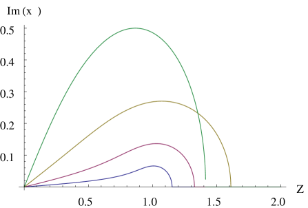
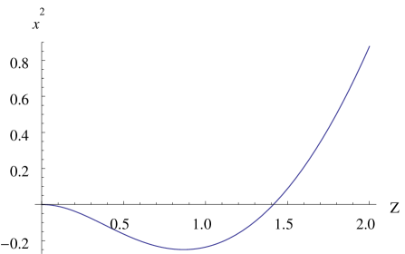
Figure 9: Left: Plot of Im$(x)$ in terms of $Z$ for $\alpha=10^{-3},10^{-2},10^{-1}$ and 1. Right: Plot of Eq. (19), $x^{2}=1+Z^{2}-\sqrt{1+4Z^{2}}$. The system is unstable, $x^{2}<0$, for $Z<\sqrt{2}$.

Symmetric beams, $\alpha=1$

Eq. (11) now reads,

$$1=\frac{1}{(x-Z)^{2}}+\frac{1}{(x+Z)^{2}},$$ (18)

which can be solved exactly for all $Z$, giving

$$x^{2}=1+Z^{2}\pm\sqrt{1+4Z^{2}}.$$ (19)

For $Z<\sqrt{2}$, the solution with a minus sign is unstable (see Fig. 9), with a most unstable wave-vector $Z_{m}$ and its frequency $x_{m}$ given by

$$Z_{m}=\frac{\sqrt{3}}{2},~{}~{}~{}~{}x_{m}=0+i\frac{1}{2}.$$ (20)

For the diluted beam regime, unstable modes are plasma Langmuir waves at $\omega\sim\omega_{p}$, traveling with the beam. Things are not so clear here. The beam is no longer a perturbation. The waves have Re$(\omega)=0$, and are the modes of the full counter-streaming system “beam+plasma”, each of equal density.

To wrap-up the most unstable mode characteristics in terms of $\alpha\in[0,1]$:

• Growth-rate: Im$(\omega/\omega_{pp})=\frac{\sqrt{3}}{2^{4/3}}\alpha^{1/3}\longrightarrow\frac{1}{2}$ (Note that $\frac{\sqrt{3}}{2^{4/3}}\sim 0.68>\frac{1}{2}$).

• Frequency: Re$(\omega/\omega_{pp})=1-\frac{\sqrt{3}}{2^{4/3}}\alpha^{1/3}\longrightarrow 0$.

• Most unstable wave-vector: $Z=1\longrightarrow\frac{\sqrt{3}}{2}$.

Relativistic effects

Maxwell’s and conservation equations are the same. Euler is now (subscripts omitted),

$$m\frac{\partial(\gamma v)}{\partial t}+mv\frac{\partial(\gamma v)}{\partial x}=qE.$$ (21)

It turns out that when linearizing “$\gamma v$” instead of “$v$”, one finds,

$$\gamma v=\gamma_{0}v_{0}+v_{1}\gamma_{0}^{3}+\cdots$$ (22)

As a result, Eq. (11) is replaced by,

$$1=\frac{\alpha}{(x-Z)^{2}\gamma_{b}^{3}}+\frac{1}{(x+\alpha Z)^{2}\gamma_{p}^{3}}.$$ (23)

Intuitively, where does these $1/\gamma^{3}$ come from ? If a particle oscillates along its main direction of motion, its mass gets a $\gamma^{3}$ relativistic boost. Changing $m$ to $m\gamma^{3}$ is Eq. (7) gives the result above.

Diluted beam, $\alpha\ll 1$

Here, $\gamma_{p}\sim 1$, so that we can recycle the non-relativistic results for diluted beam, formally replacing $\alpha\rightarrow\alpha/\gamma_{b}^{3}$, i.e. $n_{b}\rightarrow n_{b}/\gamma_{b}^{3}$. The unstable modes given by Eq. (17) now reads,

$$x=\frac{\omega}{\omega_{pp}}=1-\frac{1}{2^{4/3}}\frac{\alpha^{1/3}}{\gamma_{b}}+i\frac{\sqrt{3}}{2^{4/3}}\frac{\alpha^{1/3}}{\gamma_{b}}.$$ (24)

Symmetric beams, $\alpha=1$

With two symmetric beams, the Lorentz factors are the same $\gamma_{p}=\gamma_{b}\equiv\gamma$. Equation (23) now reads,

$$1=\frac{1}{(x-Z)^{2}\gamma^{3}}+\frac{1}{(x+Z)^{2}\gamma^{3}}.$$ (25)

Here again, we just replace $x\rightarrow x\gamma^{3/2}$ and $Z\rightarrow Z\gamma^{3/2}$, and we’re formally back to the non-relativistic case. Equation (20) then gives

$$Z_{m}=\frac{\sqrt{3}}{2\gamma^{3/2}},~{}~{}~{}~{}x_{m}=0+i\frac{1}{2\gamma^{3/2}}.$$ (26)

8 Filamentation Instability - Part 1

We still consider the same counter-streaming system, but look now at perturbations with $\mathbf{k}\perp$ to the flow. With respect to the Two-stream instability ($\mathbf{k}\parallel$ to the flow), the situation is reversed: The physics is simple, but the full maths are involved. Let’s start with the physics.

Physical picture

Suppose two particle currents of same radius $a$ and density $n$ but opposite velocities $u$, perfectly overlap (Fig. 10, left). The system is charge and current neutral, in equilibrium. We now set them apart by a distance $R$ (Fig. 10, right). The first current generates a B field at the level on the second one. The field is such that the Lorentz force F produced repels the other current even more. Unstable system. We can write,

$$F=dM\frac{d^{2}R}{dt^{2}},$$ (1)

where $dM$ is the mass of the volume element. The force reads,

$$F=dq\frac{u}{c}B,$$ (2)

where $dq$ is the charge of the volume element. With a density $n$, and particles of charge $q$ and rest mass $m$, the charge $dq$ and the mass $dM$ of the volume $dV$ read respectively,

$$dq=qndV,~{}~{}\mathrm{and}~{}~{}dM=\gamma mndV,$$ (3)

where $\gamma m$ is the relativistic mass boost for transverse motion. Equation (1) now reads,

$$qndV\frac{u}{c}B=\gamma mndV\frac{d^{2}R}{dt^{2}},~{}~{}~{}~{}\mathrm{i.e,}~{}~{}~{}~{}q\frac{u}{c}B=\gamma m\frac{d^{2}R}{dt^{2}}.$$ (4)

B is the field created by the current, so that

$$B=\frac{2I}{cR},~{}~{}\mathrm{where}~{}~{}I=nqu\pi a^{2}.$$ (5)

Replacing the current $I$ by its expression, we find

$$\frac{d^{2}\xi}{dt^{2}}=\frac{\delta^{2}}{\xi},~{}~{}\mathrm{with}~{}~{}\delta=\omega_{p}\frac{\beta}{\sqrt{2\gamma}},~{}~{}\mathrm{and}~{}~{}\xi=\frac{R}{a},~{}~{}\beta=\frac{u}{c},$$ (6)

with $\omega_{p}^{2}=4\pi nq^{2}/m$. Although this equation won’t give $\xi\propto e^{\delta t}$, it does tell the system does not relax to its initial state, on a time scale $\propto\delta^{-1}$, which fits exactly the result of the linear theory. Maybe an exponential grow would be obtained starting from opposite current partially overlapping.

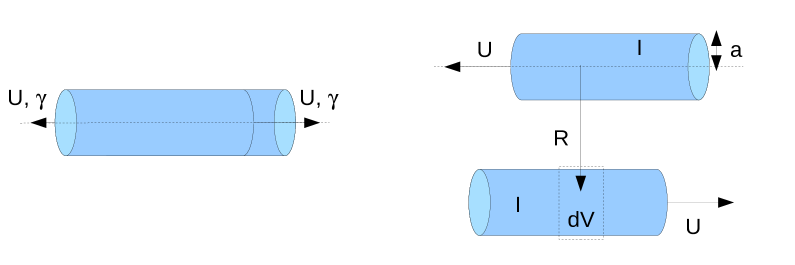
Figure 10: System unstable to the filamentation instability.

The Maths

The Dispersion Equation: Calculation Pattern

The dispersion equation for the filamentation instability is not easier to derive than the one for arbitrarily oriented $\mathbf{k}$’s. I will thus go over the general case $k_{\parallel}k_{\perp}\neq 0$, and then focus on $k_{\parallel}=0$. For the Two-stream instability, the flow of the calculation was:

Euler + Conservation eqs. (or Vlasov) for each species
$\downarrow$
First order densities $n_{1}$’s in terms of $\mathbf{E}_{1}$
$\downarrow$
Merge info for all species through Poisson’s equation
$\downarrow$
Dispersion Equation

We could use Poisson’s equation for modes with $k\parallel$ to the flow because we know they have $\mathbf{k}\parallel\mathbf{E}$. In plasma jargon, we say these modes are longitudinal, or electrostatic. For the, Poisson equation, which convert a vectorial into a scalar identity, doesn’t result in a loss of information, precisely because $\mathbf{k}\parallel\mathbf{E}$.

For filamentation modes, we don’t know about the respective orientation of $\mathbf{k}$ and $\mathbf{E}$. The divergence of the electric field would introduce the cosine of the $\widehat{\mathbf{k},\mathbf{E}}$ angle, which is unknown. Poisson’s $\nabla\cdot\mathbf{E}=4\pi\rho$ gives $k_{x}E_{x}+k_{y}E_{y}+k_{z}E_{z}=4\pi\rho$, which cannot be used as a dispersion equation because it yields only one equation for three components of the field. We need a 3D “merging species” equation which does not result in information loss. This is Maxwell-Ampère, which merges the currents instead of the charges.

The general pattern of the calculation is indeed quite similar:

Euler + Conservation eqs. (or Vlasov) for each species
$\downarrow$
First order currents $\mathbf{J}_{1}$’s in terms of $\mathbf{E}_{1}$
$\downarrow$
Merge info for all species through Maxwell-Ampère equations
$\downarrow$
Dispersion Equation

Let’s see this more in details, reasoning again from the fluid equations. Every equilibrium quantities are now slightly perturbed with terms $\propto\exp(i\mathbf{k}\cdot\mathbf{r}-i\omega t)$. The linearized conservation equations give for each species:

$$n_{1}=n_{0}\frac{\mathbf{k}\cdot\mathbf{v}_{1}}{\omega-\mathbf{k}\cdot\mathbf{v}_{0}}.$$ (7)

The linearized non-relativistic (so far) Euler equation give, still for each species:

$$\mathbf{v}_{1}=\frac{-iq/m}{\omega-\mathbf{k}\cdot\mathbf{v}_{0}}\left(\mathbf{E}_{1}+\frac{\mathbf{v}_{0}\times\mathbf{B}_{1}}{c}\right).$$ (8)

It is easy to eliminate $\mathbf{B}_{1}$ through Maxwell-Faraday equation,

$$\mathbf{B}_{1}=\frac{c}{\omega}\mathbf{k}\times\mathbf{E}_{1},$$ (9)

so that we see how Eqs. (7,8) eventually give $n_{1}$ and $\mathbf{v}_{1}$ in terms of $\mathbf{E}_{1}$ alone, for each species,

$$\mathbf{v}_{1} = \frac{-iq/m}{\omega-\mathbf{k}\cdot\mathbf{v}_{0}}\left(\mathbf{E}_{1}+\frac{\mathbf{v}_{0}\times(\mathbf{k}\times\mathbf{E}_{1})}{\omega}\right),$$

$$n_{1} = \frac{-iqn_{0}}{m}\frac{\mathbf{k}}{(\omega-\mathbf{k}\cdot\mathbf{v}_{0})^{2}}\cdot\left(\mathbf{E}_{1}+\frac{\mathbf{v}_{0}\times(\mathbf{k}\times\mathbf{E}_{1})}{\omega}\right).$$ (10)

We may now write Maxwell-Ampère equation, to merge the information from all the species into one single equation depending of $\mathbf{E}_{1}$ only,

$$i\mathbf{k}\times\mathbf{B}_{1}=\frac{-i\omega}{c}\mathbf{E}_{1}+\frac{4\pi}{c}\mathbf{J}_{1},$$ (11)

and eliminate $\mathbf{B}_{1}$ from Maxwell-Faraday Eq. (9) to obtain,

$$\frac{c^{2}}{\omega^{2}}\mathbf{k}\times(\mathbf{k}\times\mathbf{E}_{1})+\mathbf{E}_{1}+\frac{4i\pi}{\omega}\mathbf{J}_{1}=0.$$ (12)

The first order current is finally expressed through,

$$\mathbf{J}_{1}=\underbrace{n_{0,b}\mathbf{v}_{1,b}+n_{1,b}\mathbf{v}_{0,b}}_{\mathrm{Beam~{}part}}+\underbrace{n_{0,p}\mathbf{v}_{1,p}+n_{1,p}\mathbf{v}_{0,p}}_{\mathrm{Plasma~{}part}}.$$ (13)

Although the end result is not really “user friendly”, we can see how Eqs. (The Dispersion Equation: Calculation Pattern,12,13) eventually yield a tensorial equation of the form

$$\mathbf{T}\cdot\mathbf{E}_{1}=0.$$ (14)

When starting from the Vlasov equation, linearization gives the first order distribution function for each species,

$$f_{1}(\mathbf{k},\mathbf{v},\omega)=\frac{iq/m}{\omega-\mathbf{k}\cdot\mathbf{v}}\left(\mathbf{E}_{1}+\frac{\mathbf{v}\times\mathbf{B}_{1}}{c}\right)\cdot\frac{\partial f_{0}}{\partial\mathbf{v}}.$$ (15)

Here again, Maxwell-Faraday Eq. (9) together with $n_{1}=\int f_{1}dv$ and $\mathbf{v}_{1}=\int f_{1}\mathbf{v}dv$, allow to reach the dispersion equation.

9 Filamentation Instability - Part 2

Dispersion Equation Analysis

The tensorial equation $\mathbf{T}\cdot\mathbf{E}_{1}$ at the end of Plasma Talk 8 has the obvious solution $\mathbf{E}_{1}=0$. Now, the proper modes of our system are precisely the non-trivial solutions $\mathbf{T}\cdot\mathbf{E}_{1}=0$, with $\mathbf{E}_{1}\neq 0$.

That tells us two things:

• If $(\exists~{}\mathbf{E}_{1}\neq 0~{}/~{}\mathbf{T}\cdot\mathbf{E}_{1}=0)\Rightarrow\det\mathbf{T}=0$. That’s the dispersion equation, yielding $\omega$ in terms of $\mathbf{k}$.
  Assume we pick up one wave vector $\mathbf{k}$. The dispersion equation

  $$\det\mathbf{T}(\mathbf{k},\omega)=0,$$ (1)

  gives one or more $\omega$’s, $(\omega_{1,\mathbf{k}},\ldots,\omega_{N,\mathbf{k}})\in\mathbb{C}^{N}$. Each couple $(\mathbf{k},\omega_{j,\mathbf{k}})$ defines a proper mode of the system. Unstable modes have Im$(\omega)<0$.
  The fluid model usually gives a polynomial dispersion equation. Each new ingredient to the model (mobile ions, magnetic field,…), adds waves. Polynomial of degree larger than 10 are common.

• The proper modes of the system $\mathbf{E}_{1}(\mathbf{k},\omega)$ are in the Kernel of T, which is precisely the set of non-zero $\mathbf{E}_{1}$’s fulfilling $\mathbf{T}\cdot\mathbf{E}_{1}=0$.
  Assume again we picked up one wave vector $\mathbf{k}$. The dispersion equation gives a series of frequencies $(\omega_{1,\mathbf{k}},\ldots,\omega_{N,\mathbf{k}})$. We thus have $N$ tensors with vanishing determinants. Each of these $N$ tensors has a Kernel of dimension 1 or 2 (a Kernel of dimension 3 would imply T=0).

  $$\mathbf{T}(\mathbf{k},\omega_{1,\mathbf{k}})~{}~{} \Rightarrow ~{}~{}\left\{\mathbf{E}_{1,i}\left(\mathbf{k},\omega_{1,\mathbf{k}}\right)\right\}_{i=1~{}\mathrm{or}~{}2},$$

  $$\vdots$$

  $$\mathbf{T}(\mathbf{k},\omega_{N,\mathbf{k}})~{}~{} \Rightarrow ~{}~{}\left\{\mathbf{E}_{1,i}(\mathbf{k},\omega_{N,\mathbf{k}})\right\}_{i=1~{}\mathrm{or}~{}2},$$

  So, for one couple $(\mathbf{k},\omega_{\mathbf{k}})$, the formalism tells how is the $\mathbf{E}_{1}$ field. It lies either along a given direction, or in a plane. In particular, the formalism tells us about the $\widehat{\mathbf{k},\mathbf{E}}$ angle. We don’t have to assume waves are longitudinal ($\mathbf{k}\parallel\mathbf{E}$), or transverse ($\mathbf{k}\perp\mathbf{E}$). The formalism decides for us.

Figure 11: Axis conventions.

For a flow $\parallel\mathbf{z}$, and $\mathbf{k}=(k_{x},0,k_{z})$ as pictured on Fig. 11, the final form of the tensor T is given by,

$$\mathbf{T}=\left|\begin{array}[]{ccc}\eta^{2}\varepsilon_{xx}-k_{z}^{2}&0&\eta^{2}\varepsilon_{xz}+k_{z}k_{x}\\ 0&\eta^{2}\varepsilon_{yy}-k^{2}&0\\ \eta^{2}\varepsilon_{xz}+k_{x}k_{z}&0&\eta^{2}\varepsilon_{zz}-k_{x}^{2}\end{array}\right|,$$ (2)

where $\eta=\omega/c$ and $\varepsilon_{\alpha\beta}$ is given by Eq. (8) of the Review Paper.

Two-stream Check

Let’s check our assumption from Plasma Talk 7, that for $\mathbf{k}\parallel$ flow, i.e. $k_{x}=0$, there are longitudinal modes with $\mathbf{k}\parallel\mathbf{E}$. Setting $k_{x}=0$ in Eq. (2) gives,

$$\mathbf{T}(k_{z},k_{x}=0)=\left|\begin{array}[]{ccc}\eta^{2}\varepsilon_{xx}-k^{2}&0&\eta^{2}\varepsilon_{xz}\\ 0&\eta^{2}\varepsilon_{yy}-k^{2}&0\\ \eta^{2}\varepsilon_{xz}&0&\eta^{2}\varepsilon_{zz}\end{array}\right|.$$ (3)

For such wave vectors, the system is perfectly symmetric around the flow axis $z$. We thus have $\varepsilon_{xx}=\varepsilon_{yy}\equiv\varepsilon_{\perp}$, and $\varepsilon_{xz}=0$, so that

$$\mathbf{T}(k_{z},k_{x}=0)=\left|\begin{array}[]{ccc}\eta^{2}\varepsilon_{\perp}-k^{2}&0&0\\ 0&\eta^{2}\varepsilon_{\perp}-k^{2}&0\\ 0&0&\eta^{2}\varepsilon_{zz}\end{array}\right|.$$ (4)

The equation $\mathbf{T}\cdot\mathbf{E}_{1}=0$ defines two kinds of waves:

• Assume $(\mathbf{k},\omega)$ fulfills,

  $$\varepsilon_{\perp}=k^{2}c^{2}/\omega^{2},$$ (5)

  then, $\varepsilon_{zz}$ will in general not vanish for the same $(\mathbf{k},\omega)$. For these $(\mathbf{k},\omega)$, the tensor will thus have the form,

  $$\mathbf{T}=\left|\begin{array}[]{ccc}0&0&0\\ 0&0&0\\ 0&0&\eta^{2}\varepsilon_{zz}\neq 0\end{array}\right|,$$ (6)

  and waves with with $\mathbf{E}_{1}\in(x,y)$ satisfy $\mathbf{T}\cdot\mathbf{E}_{1}=0$. Since $\mathbf{k}=(0,0,k_{z})$, these are transverse modes, $\mathbf{k}\perp\mathbf{E}_{1}$. In general, they are stable.

• If we consider now $(\mathbf{k},\omega)$ fulfilling

  $$\varepsilon_{zz}=0,$$ (7)

  we find non-zero solutions of $\mathbf{T}\cdot\mathbf{E}_{1}=0$ are waves with $\mathbf{E}_{1}\in(z)$, as the tensor now takes the form,

  $$\mathbf{T}=\left|\begin{array}[]{ccc}\eta^{2}\varepsilon_{\perp}-k^{2}\neq 0&0&0\\ 0&\eta^{2}\varepsilon_{\perp}-k^{2}\neq 0&0\\ 0&0&0\end{array}\right|.$$ (8)

  Since $\mathbf{k}=(0,0,k_{z})$, these are longitudinal modes, $\mathbf{k}\parallel\mathbf{E}_{1}$, with dispersion equation,

  which indeed are our two-stream modes. It is thus checked that the modes we investigated in Plasma Talk 7 do exist.

The Filamentation Instability

About the Dispersion Equation

Let’s now consider $k_{z}=0$ in Eq. (2). We find,

$$\mathbf{T}=\left|\begin{array}[]{ccc}\eta^{2}\varepsilon_{xx}&0&\eta^{2}\varepsilon_{xz}\\ 0&\eta^{2}\varepsilon_{yy}-k^{2}&0\\ \eta^{2}\varepsilon_{xz}&0&\eta^{2}\varepsilon_{zz}-k^{2}\end{array}\right|,$$ (9)

where $\mathbf{T}\cdot\mathbf{E}_{1}=0$ again defines two kinds of modes:

• Modes with $\mathbf{E}_{1}\in(y)$, therefore transverse since $\mathbf{k}\parallel\mathbf{x}$, with dispersion equation,

  $$\varepsilon_{yy}=k^{2}c^{2}/\omega^{2}.$$ (10)

• The Filamentation modes (at last), with $\mathbf{E}_{1}\in(x,z)$ and dispersion equation,

  $$\varepsilon_{xx}(\varepsilon_{zz}-k^{2}c^{2}/\omega^{2})=\varepsilon_{xz}.$$ (11)

Of course, we would like to have $\varepsilon_{xz}=0$, which would ease our life and give a simpler, two branches dispersion equation,

$$\varepsilon_{xx} = 0,$$

$$\varepsilon_{zz} = k^{2}c^{2}/\omega^{2}.$$ (12)

Eq. (12) has been frequently used in the literature to study the Filamentation instability. It defines purely transverse waves with $\mathbf{E}_{1}\in(z)$, that is, $\parallel$ to the flow. The problem is that these papers never say they assume $\varepsilon_{xz}=0$. In general, they are wrong.

I wrote “in general”, because on rare occasions, they study settings for which truly, $\varepsilon_{xz}=0$. Which are they? Remember that even if we now focus on $\mathbf{k}=(k_{x},0,0)$, this tensor element still depends on the beam and plasma distribution functions. A detailed study shows $\varepsilon_{xz}$ strictly vanishes only if our counter streaming species are perfectly symmetric.

So, unless our density ratio is 1, and we have the same temperatures on the beam and the plasma, the same Lorentz factors, the same…  everything, the correct dispersion equation is Eq. (11), not (12).

Cold Analysis - Relativistic effects

What we’ve said is so far non-relativistic. Still in the fluid model, the main relativistic effect is displayed when linearizing the Euler equation. The relativistic Euler equation reads,

$$\frac{\partial\mathbf{p}}{\partial t}+(\mathbf{v}\cdot\nabla)\mathbf{p}=q\left(\mathbf{E}+\frac{\mathbf{v}\times\mathbf{B}}{c}\right),~{}~{}\mathbf{p}=\gamma m\mathbf{v}.$$ (13)

Its two linearized versions are,

$$im(\mathbf{k}\cdot\mathbf{v}_{0}-\omega)\mathbf{v}_{1} = q\left(\mathbf{E}_{1}+\frac{\mathbf{v}_{0}\times\mathbf{B}_{1}}{c}\right),~{}~{}~{}non-relativistic,$$

$$im(\mathbf{k}\cdot\mathbf{v}_{0}-\omega)\left(\gamma_{0}\mathbf{v}_{1}+\gamma_{0}^{3}\frac{\mathbf{v}_{1}\cdot\mathbf{v}_{0}}{c^{2}}\mathbf{v}_{0}\right) = q\left(\mathbf{E}_{1}+\frac{\mathbf{v}_{0}\times\mathbf{B}_{1}}{c}\right),~{}~{}~{}relativistic.$$ (14)

Everything is in the anisotropic linearization of $\gamma_{0}\mathbf{v}$ around $\mathbf{v}_{0}$. We see above that for a small motion along the flow, the relativistic mass increase goes like $\gamma_{0}^{3}$. But for small motion normal to the flow, $\mathbf{v}_{1}\cdot\mathbf{v}_{0}=0$ and the mass increase only goes with $\gamma$. This of course, adds a level of complexity to the general calculation, as Eq. (10) from Plasma Talk 8 for $\mathbf{v}_{1}$ is even more involved.

For the filamentation instability, we have $\mathbf{v}_{1}\cdot\mathbf{v}_{0}=0$, and we find we can just formally replace $m\rightarrow\gamma m$. Assuming a cold beam with density $n_{b}$, Lorentz factor $\gamma_{b}$, and cold plasma electrons with density $n_{p}$ and Lorentz factor $\gamma_{p}$, the tensor elements are,

$$\varepsilon_{xx} = 1-\frac{\alpha}{x^{2}\gamma_{b}}-\frac{1}{x^{2}\gamma_{p}},$$

$$\varepsilon_{yy} = 1-\frac{\alpha}{x^{2}\gamma_{b}}-\frac{1}{x^{2}\gamma_{p}},$$

$$\varepsilon_{zz} = 1-\frac{\alpha}{x^{2}\gamma_{b}}-\frac{\alpha Z^{2}}{x^{4}\gamma_{b}}-\frac{1}{x^{2}\gamma_{p}}-\frac{\alpha^{2}Z^{2}}{x^{4}\gamma_{p}},$$

$$\varepsilon_{xz} = \frac{\alpha Z}{x^{3}\gamma_{p}}\left(\frac{1}{\gamma_{p}}-\frac{1}{\gamma_{b}}\right),$$ (15)

with again,

$$x=\frac{\omega}{\omega_{pp}},~{}~{}~{}~{}Z=\frac{kv_{b}}{\omega_{pp}},~{}~{}~{}\alpha=\frac{n_{b}}{n_{p}}.$$ (16)

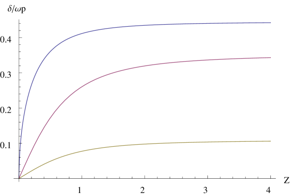
Figure 12: Filamentation instability growth-rate for density ratios $\alpha=1$, 0.5 and 0.1, from higher to lower curves respectively. The beam Lorentz factor is $\gamma_{b}=10$.

The numerical resolution of Eq. (11), when plugging the tensor elements above, yields the growth-rate curves pictured on Fig. 12. As evidenced, the growth-rate just saturates for large $Z$. A trick to recover the large $Z$ growth-rate, consists in extracting the coefficient $a_{n}$ of $Z^{n}$ in the polynomial dispersion equation, as $a_{n}=0$ is the asymptotic dispersion equation for $Z\rightarrow\infty$. Doing so, one finds a zero real frequency and

$$\lim_{Z\rightarrow\infty}\frac{\delta}{\omega_{pp}} = \frac{v_{b}}{c}\sqrt{\frac{\alpha}{\gamma_{b}}},~{}~{}~{}\alpha\ll 1,$$ (17)

$$= \frac{v_{b}}{c}\sqrt{\frac{2}{\gamma_{b}}},~{}~{}~{}\alpha=1,$$ (18)

where the agreement with Eq. (6) of Plasma Talk 8 can be checked. Note that for $\alpha=1$, the tensor elements (Cold Analysis - Relativistic effects) simplify substantially. Equation (12) for unstable modes is valid and reads,

$$x^{2}-\frac{2}{\gamma_{b}^{3}}-\frac{2Z_{x}^{2}}{x^{2}\gamma_{b}}=\frac{Z_{x}^{2}}{\beta^{2}},$$ (19)

which can be solved exactly.

We can follow the same line of reasoning for the “wrong” transverse dispersion equation (12), in order to check its inaccuracy. The exact result is for any $\alpha$,

$$\lim_{Z\rightarrow\infty}\frac{\delta_{T}}{\omega_{pp}}=\beta\sqrt{\frac{\alpha(\alpha\gamma_{b}+\gamma_{p})}{\gamma_{b}\gamma_{p}}} = \beta\sqrt{\frac{\alpha(\alpha\gamma_{b}+1)}{\gamma_{b}}},~{}~{}~{}\alpha\ll 1,$$ (20)

$$= \beta\sqrt{\frac{2}{\gamma_{b}}},~{}~{}~{}\alpha=1.$$ (21)

As expected, the result for the symmetric case $\alpha=1$ is the same. But for the diluted beam regime $\alpha\ll 1$, the “transverse” growth-rate $\delta_{T}$ differs from the exact one by,

$$\delta_{T}=\delta\sqrt{1+\alpha\gamma_{b}},$$ (22)

so that the transverse calculation overestimates the growth-rate by a factor which can be arbitrarily large.

10 Oblique Modes

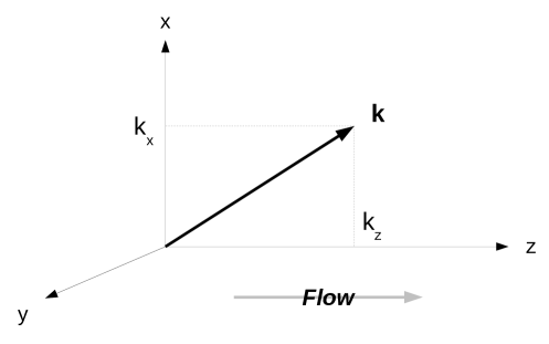
Figure 13: Axis conventions and setup.

The electrostatic approximation

We now come to these fast growing “oblique” modes in the relativistic regime. They are found for both $k_{\parallel}\neq 0$ and $k_{\perp}\neq 0$, thus their name.

Let’s remind the general dispersion equation for a set-up like to one pictured on Fig. 13. From Eqs. (1,2) of Plasma Talk 9, we have the dispersion equation

$$\det\mathbf{T}(\mathbf{k},\omega)=0,$$ (1)

with,

$$\mathbf{T}=\left|\begin{array}[]{ccc}\eta^{2}\varepsilon_{xx}-k_{z}^{2}&0&\eta^{2}\varepsilon_{xz}+k_{z}k_{x}\\ 0&\eta^{2}\varepsilon_{yy}-k^{2}&0\\ \eta^{2}\varepsilon_{xz}+k_{x}k_{z}&0&\eta^{2}\varepsilon_{zz}-k_{x}^{2}\end{array}\right|,$$ (2)

where $\eta=\omega/c$ and $\varepsilon_{\alpha\beta}$ is given by Eq. (8) of the Review Paper. We could just go on with this expression, plug some distribution functions for the beam and the plasma, and solve the dispersion equation. Doing so, we would realize something important for these oblique modes: unless we’re really close the $k_{\parallel}=0$, these modes have $\mathbf{k}\times\mathbf{E}\sim\mathbf{0}$. That had already been noticed long ago in the first papers on the topic, for the cold case. That’s been confirmed recently for the hot case with various distribution functions, but to my knowledge, it hasn’t been proved from the formalism.

It is then fruitful to assume $\mathbf{k}\times\mathbf{E}=\mathbf{0}$. Although this approximation breaks down for k near the normal direction, it has so far been found valid for the fastest growing oblique mode. The approximation is called the “electrostatic” or “longitudinal” approximation.

Poisson’s equation can still deliver a dispersion equation, but in a slighter intricate way because of relativistic effects (a derivation from Ampère’s equation, similar to the filamentation one, is exposed in the Appendix). We simply go through the calculations of Plasma Talk 8 & 9, assuming at each steps $\mathbf{k}\times\mathbf{E}_{1}=\mathbf{0}$, implying $\mathbf{B}_{1}=\mathbf{0}$ as well.

The relativistic linearized conservation and Euler equations give for each species,

$$n_{1} = n_{0}\frac{\mathbf{k}\cdot\mathbf{v}_{1}}{\omega-\mathbf{k}\cdot\mathbf{v}_{0}}$$

$$m\left(\gamma_{0}\mathbf{v}_{1}+\gamma_{0}^{3}\frac{\mathbf{v}_{1}\cdot\mathbf{v}_{0}}{c^{2}}\mathbf{v}_{0}\right) = q\left(\mathbf{E}_{1}+\cancel{\frac{\mathbf{v}_{0}\times\mathbf{B}_{1}}{c}}\right).$$ (3)

Solving these two equations gives for the perturbed density,

$$n_{1}=i\frac{k_{z}E_{1z}+\gamma^{2}k_{x}E_{1x}}{(\omega-\mathbf{k}\cdot\mathbf{v}_{0})^{2}}.$$ (4)

Inputs from each species are then merged through Poisson’s equation,

$$\mathbf{k}\cdot\mathbf{E}_{1}=\omega_{pb}^{2}\frac{k_{z}E_{1z}+\gamma_{b}^{2}k_{x}E_{1x}}{(\omega-\mathbf{k}\cdot\mathbf{v}_{0b})^{2}}+\omega_{pp}^{2}\frac{k_{z}E_{1z}+\gamma_{p}^{2}k_{x}E_{1x}}{(\omega-\mathbf{k}\cdot\mathbf{v}_{0p})^{2}},$$ (5)

which may be put under the form $\mathbf{W}\cdot\mathbf{E}_{1}=0$, where the vector $\mathbf{W}$ reads,

$$\mathbf{W}=\left(\begin{array}[]{c}k_{x}\\ 0\\ k_{z}\end{array}\right)-\frac{\omega_{pb}^{2}}{(\omega-\mathbf{k}\cdot\mathbf{v}_{0b})^{2}}\left(\begin{array}[]{c}\gamma_{b}^{2}k_{x}\\ 0\\ k_{z}\end{array}\right)-\frac{\omega_{pp}^{2}}{(\omega-\mathbf{k}\cdot\mathbf{v}_{0p})^{2}}\left(\begin{array}[]{c}\gamma_{p}^{2}k_{x}\\ 0\\ k_{z}\end{array}\right).$$ (6)

Now, $\mathbf{k}\parallel\mathbf{E}_{1}$ and $\mathbf{W}\cdot\mathbf{E}_{1}=0$, implies $\mathbf{W}\cdot\mathbf{k}=0$, which gives,

$$1-\frac{k_{z}^{2}+k_{x}^{2}\gamma_{b}^{2}}{k_{z}^{2}+k_{x}^{2}}\frac{\omega_{pb}^{2}/\gamma_{b}^{3}}{(\omega-k_{z}v_{b})^{2}}-\frac{k_{z}^{2}+k_{x}^{2}\gamma_{p}^{2}}{k_{z}^{2}+k_{x}^{2}}\frac{\omega_{pp}^{2}/\gamma_{p}^{3}}{(\omega-k_{z}v_{p})^{2}}=0.$$ (7)

Note that in this longitudinal approximation, there are no oblique effects for $\gamma_{b}=\gamma_{p}=1$. A generalization of the result to the kinetic level is not as obvious as in the 1D theory for the two-stream instability, precisely because we are not 1D. The kinetic equation reads,

$$0=1+\frac{4\pi q^{2}}{k^{2}}\int\frac{\mathbf{k}\cdot\partial f_{0}(\mathbf{p})/\partial\mathbf{p}}{\omega-\mathbf{k}\cdot\mathbf{v}}d^{3}p,~{}~{}~{}~{}\mathbf{p}\frac{m\mathbf{v}}{\sqrt{1-v^{2}/c^{2}}}.$$ (8)

It should not be very difficult to derive intuitively Eq. (8) from Eq. (7) summing the beamlets contributions, as we did for the 1D case. In terms of the usual dimensionless variables,

$$x=\frac{\omega}{\omega_{pp}},~{}~{}~{}~{}Z=\frac{kv_{b}}{\omega_{pp}},~{}~{}~{}\alpha=\frac{n_{b}}{n_{p}},$$ (9)

and using $v_{p}=-\alpha v_{b}$, Eq. (7) reads,

$$0=1-\underbrace{\frac{Z_{z}^{2}+\gamma_{b}^{2}Z_{x}^{2}}{Z_{z}^{2}+Z_{x}^{2}}\frac{\alpha/\gamma_{b}^{3}}{(x-Z_{z})^{2}}}_{beam}-\underbrace{\frac{Z_{z}^{2}+\gamma_{p}^{2}Z_{x}^{2}}{Z_{z}^{2}+Z_{x}^{2}}\frac{1/\gamma_{p}^{3}}{(x+Z_{z}\alpha)^{2}}}_{plasma}.$$ (10)

Diluted beam

For $\alpha\ll 1$, $\gamma_{p}\sim 1$ and Eq. (10) reads,

$$0=1-\frac{Z_{z}^{2}+\gamma_{b}^{2}Z_{x}^{2}}{Z_{z}^{2}+Z_{x}^{2}}\frac{\alpha/\gamma_{b}^{3}}{(x-Z_{z})^{2}}-\frac{1}{(x+Z_{z}\alpha)^{2}}.$$ (11)

This equation is very similar to the one we found for the diluted two-stream case (non-relativistic). We formally deal with a diluted beam of equivalent density ratio,

$$\alpha^{\prime}=\frac{\alpha}{\gamma_{b}^{3}}~{}\frac{Z_{z}^{2}+\gamma_{b}^{2}Z_{x}^{2}}{Z_{z}^{2}+Z_{x}^{2}}.$$ (12)

The maximum growth rate will be found for $Z_{z}\sim 1$, and the frequency of the unstable mode reads,

$$\Im(x) = \frac{\sqrt{3}}{2^{4/3}}\frac{\alpha^{1/3}}{\gamma_{b}}\left(\frac{1+\gamma_{b}^{2}Z_{x}^{2}}{1+Z_{x}^{2}}\right)^{1/3},$$ (13)

$$\Re(x) = 1-\frac{1}{2^{4/3}}\frac{\alpha^{1/3}}{\gamma_{b}}\left(\frac{1+\gamma_{b}^{2}Z_{x}^{2}}{1+Z_{x}^{2}}\right)^{1/3}.$$

The growth rate (13) displays THE oblique effect: For perp components of the wave vector such that $\gamma_{b}^{2}Z_{x}^{2}\gg 1$, we switch from a $\gamma_{b}^{-1}$ to a $\gamma_{b}^{-1/3}$ scaling.

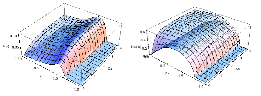
Figure 14: LEFT: Exact growth rate from dispersion equation (18) (transparent) vs. longitudinal for $\alpha=10^{-2}$ and $\gamma_{b}=3$. RIGHT: Same for $\alpha=1$ and $\gamma_{b}=1.1$.

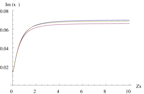
Figure 15: Comparison of the exact growth rate (top, blue curve), the longitudinal result (lower, purple curve) and Eq. (13) [middle, yellow curve] along the perp $Z_{x}$ direction at fixed $Z_{z}=1$. The density ratio is $\alpha=0.01$ and the beam Lorentz factor $\gamma_{b}=10$.

The validity of the longitudinal approximation is tested on Fig. 14 where it is compared to the exact solution. As expected, it breaks down for small $Z_{z}$ while the exact calculation renders the filamentation growth rate as well.

Fixing $Z_{z}=1$, we can compare the exact solution, the longitudinal result and Eq. (13) along the perp $Z_{x}$ direction. The result is displayed on Fig. 15.

Symmetric beams

For $\alpha=1$, $\gamma_{b}=\gamma_{p}\equiv\gamma$ and Eq. (10) reads,

$$0=1-\frac{1}{(x-Z_{z})^{2}\Gamma^{3}}-\frac{1}{(x+Z_{z})^{2}\Gamma^{3}},~{}~{}~{}~{}\Gamma=\gamma\left(\frac{Z_{z}^{2}+Z_{x}^{2}}{Z_{z}^{2}+\gamma^{2}Z_{x}^{2}}\right)^{1/3}.$$ (14)

With an equation formally equivalent to the one studied for the two-stream symmetric case in Plasma Talk 7. Although the equation above can be exactly solved for $x$, studying the fastest growing $Z_{z}$ for any given $Z_{x}$ is difficult because both are eventually inside $\Gamma$. Once the equation is solved, we can however look at the large $Z_{x}$ limit of the growth rate which reads,

$$\delta^{2}_{Z_{x}\rightarrow\infty}=\frac{1+Z_{z}^{2}\gamma_{b}-\sqrt{1+4Z_{z}^{2}\gamma_{b}}}{\gamma_{b}},$$ (15)

reaching the extremum,

$$\delta_{m,Z_{x}\rightarrow\infty}=\frac{1}{2\sqrt{\gamma_{b}}},~{}~{}~{}\mathrm{for}~{}~{}~{}~{}Z_{z,m}=\frac{\sqrt{3}}{2\sqrt{\gamma_{b}}}.$$ (16)

Exact dispersion equation

Without the longitudinal approximation, and for arbitrarily oriented $\mathbf{k}$’s, we are back to the determinant of the tensor (2) for the dispersion equation. It has two branches corresponding to the two factors of the determinant,

$$\varepsilon_{yy}=k^{2}c^{2}/\omega^{2} ~{}~{}~{}\mathbf{E}_{1}\in(y),$$ , (17)

$$(\eta^{2}\varepsilon_{xx}-k_{z}^{2})(\eta^{2}\varepsilon_{zz}-k_{x}^{2})=(\eta^{2}\varepsilon_{xz}-k_{x}k_{z})^{2} ~{}~{}~{}\mathbf{E}_{1}\in(x,z).$$ , (18)

The second branch therefore holds the two-stream, the oblique and the filamentation instabilities. As evidenced by the exact plot on Figs. 14, there is a continuous transition from two-stream to filamentation modes, probably linked to a common underlying physics. Any ideas ?

Cold hierarchy

We may finally establish the hierarchy of modes for the cold regime in the $(\alpha,\gamma_{b})$ phase space. The competing modes, with their variation from $\alpha\ll 1$ to 1, are

$$\mathrm{Two-stream},~{}~{}\Im(x) = \frac{\sqrt{3}}{2^{4/3}}\frac{\alpha^{1/3}}{\gamma_{b}}\rightarrow\frac{1}{2\gamma_{b}^{3/2}},$$

$$\mathrm{Oblique},~{}~{}\Im(x) = \frac{\sqrt{3}}{2^{4/3}}\left(\frac{\alpha}{\gamma_{b}}\right)^{1/3}\rightarrow\frac{\sqrt{3}}{2\gamma_{b}^{1/2}},$$

$$\mathrm{Filamentation},~{}~{}\Im(x) = \frac{v_{b}}{c}\sqrt{\frac{\alpha}{\gamma_{b}}}\rightarrow\frac{v_{b}}{c}\sqrt{\frac{2}{\gamma_{b}}}.$$ (19)

The Two-stream case is quickly settled: it is always slower than the oblique unless $\gamma_{b}=1$. In the cold regime, the two-stream instability never governs the unstable spectrum.

We are thus left comparing oblique and filamentation modes. For the diluted regime, the $\gamma_{b}$ scaling clearly favors the oblique. Situation is more involved near the symmetric regime. As evidenced on Fig. 14 RIGHT, the longitudinal approximation gives the good order of magnitude for the growth rate, but is not enough to render the “fine structure” of the problem.

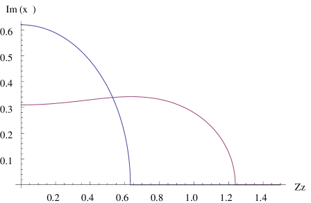
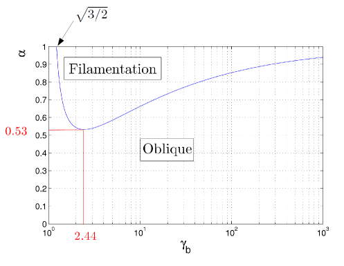
Figure 16: LEFT: Growth rate $Z_{x}\rightarrow\infty$ in terms of the parallel wave vector $Z_{z}$, for $\gamma_{b}=5$, and $\alpha=0.3$ and 1 (lower and upper curves respectively). The local oblique extremum vanishes when approaching the symmetric case. RIGHT: Dominant mode in terms of $(\gamma_{b},\alpha)$.

What is this “fine structure”? In the diluted beam regime, we clearly have a local extremum for oblique vectors corresponding to oblique modes. When approaching the symmetric regime, this may no longer be the case. To evidence this, we’ve plotted on Fig. 16 LEFT the growth rate at $Z_{x}\rightarrow\infty$ for different parameters. For $\alpha=0.3$, we clearly find an oblique extremum, which turns to be the dominant mode. But in the symmetric case $\alpha=1$, the local extremum disappears, giving rise to a monotonous behavior and a system governed by filamentation.

As a consequence, the oblique/filamentation frontier has to be determined numerically for large density ratios. The resulting hierarchy plot can be found on Fig. 16, RIGHT. The frontier position for $\alpha=1$ can be determined exactly from the dispersion equation at $Z_{x}\rightarrow\infty$. At $\alpha=1$, the equation can be solved, and the local oblique extremum vanishes when the second derivative of the growth rate at $Z_{z}=0$ vanishes. For $\alpha\neq 1$, this second derivative vanishes on the blue line. Note the frontier gets closer to $\alpha=1$ for large $\gamma_{b}$’s, with a convergence numerically found like $\gamma_{b}^{-0.395}$.

More detailed in the Review Paper, Section IV-A.

Appendix

We here derive the dispersion equation (7) from Maxwell-Ampère equation. The equation we used to merge information from each species, namely Eq. (12) from Plasma Talk 8 simplifies in the longitudinal approximation,

$$\cancel{\frac{c^{2}}{\omega^{2}}\mathbf{k}\times(\mathbf{k}\times\mathbf{E}_{1})}+\mathbf{E}_{1}+\frac{4i\pi}{\omega}\mathbf{J}_{1}=0.$$ (20)

From Eqs. (The electrostatic approximation,4), the first order current is expressed in terms of $\mathbf{E}_{1}$, leading again to a tensorial equation of the form,

$$\mathbf{T}\cdot\mathbf{E}_{1}=\mathbf{0}.$$ (21)

If we have but two counter-streaming species (beam + plasma), the tensor reads,

$$\mathbf{T}=\left(\begin{array}[]{ccc}\omega+\frac{\omega_{pb}^{2}}{\gamma_{b}(k_{z}v_{b}-\omega)}+\frac{\omega_{pp}^{2}}{\gamma_{p}(k_{z}v_{p}-\omega)}&0&0\\ 0&0&0\\ -k_{x}\left(\frac{v_{b}\omega_{pb}^{2}}{\gamma_{b}(k_{z}v_{b}-\omega)^{2}}+\frac{v_{p}\omega_{pp}^{2}}{\gamma_{p}(k_{z}v_{p}-\omega)^{2}}\right)&0&\omega\left(1-\frac{\omega_{pb}^{2}}{\gamma_{b}^{3}(k_{z}v_{b}-\omega)^{2}}-\frac{\omega_{pp}^{2}}{\gamma_{p}^{3}(k_{z}v_{p}-\omega)^{2}}\right)\end{array}\right).$$ (22)

The summing of elements from each species is here obvious again. Note that when $\mathbf{k}$ is aligned with the main axis, that is $k_{\perp}=0$ or $k_{\parallel}=0$, the respective orientation of $\mathbf{k}$ and $\mathbf{E}_{1}$ is easily determined, because $\mathbf{E}_{1}$ is also found along the very same main axis. Things are here different because the orientation of $\mathbf{k}$ is arbitrary while the “easy” axis of our tensor are still the main ones.

Assume we have $\mathbf{E}_{1}$ fulfilling Eq. (21) and $\mathbf{E}_{1}\parallel\mathbf{k}$. Because $\mathbf{T}$ is a linear operator, that implies $\mathbf{T}\cdot\mathbf{k}$ is also the null vector:

$$\mathbf{T}\cdot\mathbf{k}=\mathbf{0}.$$ (23)

The scalar product $\mathbf{k}\cdot(\mathbf{T}\cdot\mathbf{k})$ must therefore also vanish,

$$\mathbf{k}\cdot(\mathbf{T}\cdot\mathbf{k})=0.$$ (24)

The advantage is that the left-hand-side of Eq. (24) is now a scalar, giving us the dispersion equation for longitudinal waves with arbitrarily oriented $\mathbf{k}$’s. That quantity can be calculated from (22), and gives the dispersion equation (7).

11 Temperature Effects

I will quickly go through the main temperature, i.e. energy spread effects, on our instabilities. Let’s first start finding out about the limits of the cold regime.

When are we no longer “cold”?

The instability process is a matter of wave-particle interaction. Assume a mode $\mathbf{k}$ is exchanging energy with a group of particles. If during one growth period, all particles remain in phase with the wave, the interaction is virtually cold. The wave grows as if there was no thermal spread at all. Writing that after one growth period, the velocity spread along k produces a spatial spread smaller than the wavelength, we find the condition for the validity of the cold model,

$$\Delta v_{\mathbf{k}}~{}\delta^{-1}\ll k^{-1},$$ (1)

where $\delta$ is the growth rate. Note worthily, the condition is not homogenous throughout the $\mathbf{k}$ space. The spread $\Delta v_{\mathbf{k}}$ and the growth rate both depend on $\mathbf{k}$. A given system may be virtually cold for the two-stream instability, and hot for the filamentation.

The same physical picture allows to understand the main effect of temperature. Thermal spread reduces the growth rates, precisely because if condition (1) is not fulfilled, the wave can exchange energy only with a fraction of the particles involved in the cold regime.

See Section III.C of the Review.

Two-stream modes

Assume a 1D beam/plasma system with a velocity distribution such as the one pictured on Fig. 17 LEFT, and define the temperature parameter,

$$\rho=\frac{V_{t}}{V}.$$ (2)

For $\rho=0$, we have two counter-streaming symmetric beams. But it is obvious that if $\rho=1$, the two distributions make contact, and we end up with a total distribution equivalent to an homogenous stable plasma at rest, with velocity spread equal to $\pm 2V$.

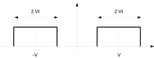
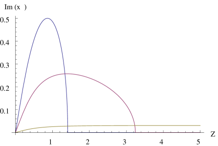
Figure 17: LEFT: Simple toy model for the stabilization of the 1D two-stream instability. RIGHT: Growth rate in terms of $Z=kV/\omega_{p}$ for $\rho=0$, 0.9 and 0.999 from higher to lower curves respectively. The system is stable for $\rho>1$.

Indeed, the dispersion equation is easily computed, and reads in terms of the usual dimensionless parameters,

$$1-\frac{1}{(x+Z)^{2}-(\rho Z)^{2}}-\frac{1}{(x-Z)^{2}-(\rho Z)^{2}}=0.$$ (3)

A plot of the growth rate is pictured on Fig. 17 RIGHT, evidencing the progressive stabilization of the system for $\rho$ approaching unity.

The same pattern holds for more realistic distribution functions. The so-called “Penrose Criterion” states that distribution functions are unstable if they have more than one local extremum. Bottom line: for hot enough beam and/or plasma, two-stream can be stabilized, relativistic or not.

Something interesting: It is tempting to relate the former criterion to the formula for Landau Damping giving a growth rate $\propto f^{\prime}_{0}(\omega/k)$. Nevertheless, we find here unstable waves with a distribution function which derivative is almost always zero! In addition, when the system is unstable for $\rho<1$, the real part of the unstable modes is found at $\omega=0$, so that $f^{\prime}_{0}(\omega/k)=0$ in our case, while there are no particles at $v=0$. This is not an artifact of our distribution functions, because $\omega=0$ also with two counter-streaming symmetric Maxwellian species.

I have never seen this kind of issues discussed, except in one single paper. There are things left to understand…

Filamentation modes

Let’s extend our toy model consisting in distributions flat up to a certain velocity (“waterbag”). Consider the 3 distribution functions pictured on Fig. 18. The shaded areas are uniformly filled with particles in velocity space.

• A is a counter-streaming system. Unstable to both two-stream and filamentation instabilities.

• In B, we just extend the parallel spread until the distributions come in contact. According to the previous paragraph, the result is two-stream stable. But the result is also anisotropic. Weibel found it is unstable to perturbations with $\mathbf{k}$ normal to the highest thermal spread: that’s filamentation here. B is therefore two-stream stable and filamentation unstable.

• C is built from B, equating the spread in every directions. The result is stable.

We thus find we can “play” with temperature parameters in order to stabilize some parts of the spectrum, or all of it. The bottom line here is that filamentation can be stabilized.

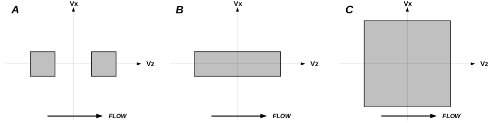
Figure 18: Distribution functions with different stability properties.

Note that in Fig. 18, we carefully tailor the spreads of every species to cancel the instability. What if we just play with the beam, that is, the component around $v_{z}>0$ on Fig. 18-A? The end result depends on the distribution:

• For waterbag distributions, filamentation is stabilized beyond a certain amount of beam transverse spread. That can be understood as follows: Assume a current filament of radius $1/k$ and density $n_{b}$. The current is $I\sim qn_{b}k^{-2}v_{b}$. It creates at the surface of the filament a field $B=2I/ck^{-1}$. A charge at the surface is therefore pulled in by the Lorentz force

  $$F_{B}=q\frac{v_{b}B}{c}=\left(\frac{v_{b}}{c}\right)^{2}q^{2}n_{b}k^{-1}.$$ (4)

  If there is no temperature, nothing prevents the filament from further pinching, which is why the instability extends up to $k=\infty$ in the cold regime. But if we’re hot, kinetic pressure opposes the pinching: A little piece of filament near the surface, with volume $dV$ and surface $dS$, is pulled in by $F_{B}n_{b}dV$, and pushed out by $n_{b}k_{B}TdS$. Pinching is prevented if,

  $$n_{b}k_{B}TdS>F_{B}n_{b}dV~{}~{}\Rightarrow~{}~{}k>q\frac{v_{b}}{c}\sqrt{\frac{n_{b}}{k_{B}T}}~{}\equiv~{}k_{m\perp}\propto\frac{\sqrt{n_{b}}}{v_{tb}},$$ (5)

  which is the scaling found from the theory with waterbag distributions (we have used $dV\sim k^{-1}dS$, and $v_{tb}$ is the thermal beam spread.).

• For relativistic Maxwellians, it has been proved that filamentation never vanishes completely. If $T_{b}$ is the beam temperature, the maximum filamentation growth-rate scales like $T_{b}^{-3/2}$. In addition, this result still holds for any plasma temperature.

Oblique modes - general thermal “rules”

Two-stream modes are unstable up to a finite $k_{m\parallel}$, and filamentation up to yet another finite $k_{m\perp}$. How do we close the unstable domain? Two different answers according to the distribution. With waterbag, we close from, and to infinity. See Fig. 10a of the Review. With a Maxwellian, these large $k$ oblique modes are stabilized, and we close “normally”, as pictured for example on Fig. 14 of the Review.

Oblique modes’ temperature sensitivity is intermediate between two-stream and filamentation. As evidenced in Plasma Talk 10, they tend to be interesting only in the relativistic regime, due to the $\gamma_{b}$ scaling which favors them. Two thermal “rules” are useful to grasp the influence of the beam spread over the full spectrum:

• Parallel spread hardly matters. Why? Because in the relativistic regime, it takes a huge parallel energy spread to get a reasonable parallel velocity spread. All velocities are squeezed against $c$. See Fig. 13 of the Review.

• Two-stream does not care about the transverse spread, because particles differing only by their transverse velocity will equally stay tuned with a plane wave at $\mathbf{k}\parallel flow$. For the same reason, filamentation do care.
  As a result, modes are all the more affected by beam temperature than they are oblique.

We could rank, from best to worst, the 3 kinds of modes in terms of the way they “resist” the various effects:

Relativistic:

Oblique $\rightarrow$ Filamentation $\rightarrow$ two-stream.

Density ratio:

Filamentation $\rightarrow$ Oblique/two-stream.

Beam temperature:

Two-stream $\rightarrow$ Oblique $\rightarrow$ Filamentation.

All this ends up with the mode hierarchy pictured on Fig. 20 of the Review Paper.

The phase velocity diagram - Fig. 17 of the Review

A great tool to understand the physics. Plot, on the very same graph, the distribution functions and the phase velocities of the unstable modes. On can straightforwardly check which species are in resonance with which kind of modes.

12 Non-Linear Regime

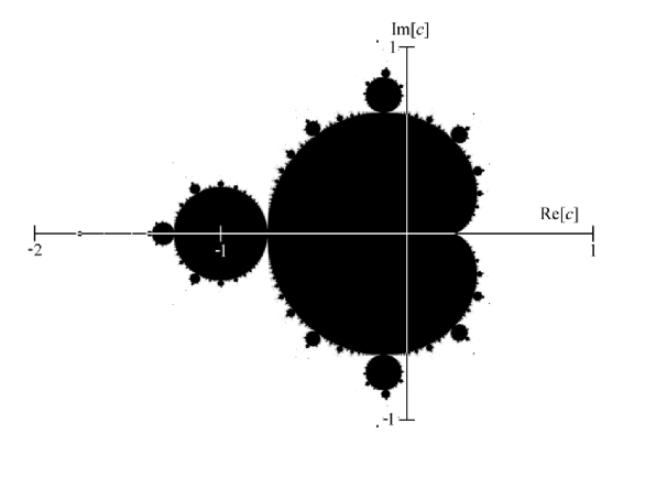
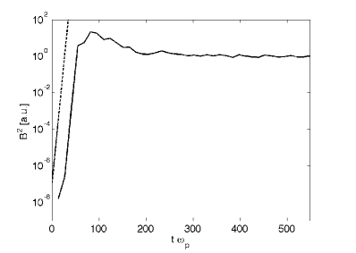
Figure 19: Left: The “Mandelbrot set”, defined by Eqs. (The phase velocity diagram - Fig. 17 of the Review,2). Right: Typical field growth extracted from a PIC simulation. Growth roughly stops when the linear exponential growth stops. The line shows the expected growth from theory.

Non-linear problems may be complicated with just 1 or 2 degrees of freedom. Think about this 2D example: take the very simple sequence

$$z_{n+1} = z_{n}^{2}+c,$$

$$z_{0} = c,~{}~{}c\in\mathbb{C},$$ (1)

and just define the set

$$M=\left\{c\in\mathbb{C}~{}/~{}\lim_{n\rightarrow\infty}\mid z_{n}\mid\neq\infty\right\}.$$ (2)

You have the famous, and incredibly complicated, fractal and everything, “Mandelbrot set” pictured on Fig. 19. People were stunned when they realized something as trivial as Eq. (The phase velocity diagram - Fig. 17 of the Review) could generate such amount of complexity.

A plasma has $\infty$ number of degrees of freedom. Yet, to my knowledge, something as beautiful as Fig. 19 is still lacking in plasma physics. Maybe because it’s too complicated…

At any rate, there’s no hope of analytically finding out about the long term evolution of our beam plasma systems in the general case. Remember it took a Fields Medal to prove non-linear Landau damping. Even for the cold case, things are not easy.

I’ll go through some results on the saturation of the various instabilities, always assuming the fastest growing mode is the only one excited, and that everything is cold at $t=0$. The former is quite reasonable, as the most unstable mode grows exponentially faster than the rest. Relativistic effects help as they drive a sharper unstable spectrum, where growth rates vary rapidly from one mode to another. The later is a limitation.

The idea is to find out when the linear theory should break down, and to claim that growth stops at that point. Granted, exponential growth should stop there. But other kind of growth could keep on. Yet the observed field growth in PIC simulations is always like to one pictured on Fig. 19. Why?

See Section V of the Review Paper, and references therein.

Two-stream and oblique instabilities

Two-stream, non-relativistic

We assume a diluted beam. There, two-stream is resonant with the beam. Say the wave $Ee^{ikx-i\omega t}$ is growing, traveling along with the beam electrons. Electrons will start oscillating in the field at the “bouncing” frequency,

$$\omega_{b}^{2}=\frac{qEk}{m}.$$ (3)

The linear assumption that all electrons have $v=v_{b}$ during one growth period $\delta^{-1}$ breaks down when,

$$\omega_{b}=\delta~{}~{}\Rightarrow~{}~{}E_{s}=\frac{\delta^{2}}{\omega_{p}}\frac{mv_{b}}{q},$$ (4)

giving the value of the field at saturation (I’ve set here $k\sim\omega_{p}/v_{b}$). A great by-product of $E_{s}$ is the beam energy loss $\Delta W_{b}$. Since the field energy can only come from the beam energy, we can write,

$$\frac{\Delta W_{b}}{\frac{1}{2}n_{b}mv_{b}^{2}} = \frac{E_{s}^{2}/8\pi}{\frac{1}{2}n_{b}mv_{b}^{2}}$$

$$= \frac{n_{p}}{n_{b}}\left(\frac{\delta}{\omega_{p}}\right)^{4}\sim\left(\frac{n_{b}}{n_{p}}\right)^{1/3},$$

where I just replaced the growth-rate by its cold value $\frac{\sqrt{3}}{2^{4/3}}(n_{b}/n_{p})^{1/3}\omega_{p}$. We could even write the energy lost is shared between the plasma and the field. In such case, $\Delta W_{b}/W_{b}$ is half the result (Two-stream, non-relativistic).

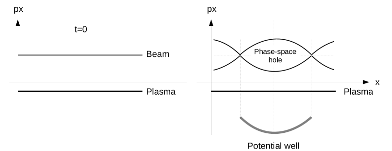
Figure 20: Phase-space hole.

As the field grows and traps the beam electrons, they start oscillating in the wave potential. PIC people love to plot density graphs in the $(x,v_{x})$ phase-space (say $x$ is our dimension) such as the one pictured on Fig. 20. At $t=0$, the beam and the plasma are just two lines. In the instability phase, the plasma does not move a lot, but the beam particles start oscillating in the wave, creating “holes” in the phase-space.

Two-stream, Relativistic

A naive reasoning gives the right answer. As the oscillatory trapping motion is along the flow, we replace $m\rightarrow\gamma_{b}^{3}m$ in the bouncing frequency (3). This gives the field at saturation,

$$E_{s}=\frac{\delta^{2}}{\omega_{p}}\frac{\gamma_{b}^{3}mv_{b}}{q}.$$ (6)

The relative energy loss is then computed as in Eq. (Two-stream, non-relativistic), replacing the growth-rate by its relativistic value. It reads,

$$\frac{\Delta W_{b}}{n_{b}\gamma_{b}mc^{2}}\sim\gamma_{b}\beta^{2}\left(\frac{n_{b}}{2n_{p}}\right)^{1/3}.$$ (7)

Of course, this quantity has to remain small since linear regime means unperturbed trajectories, that is, $\Delta W_{b}\ll W_{b}$. The energy loss eventually relies on the parameter $S$ with

$$S=\gamma_{b}\beta^{2}\left(\frac{n_{b}}{2n_{p}}\right)^{1/3}.$$ (8)

If you do the “clean” calculation going to the wave frame, like in the footnote, you need the beam dynamic in that frame to be non-relativistic in order to compute easily a bouncing frequency. Doing so requires $S\ll 1$, as explained in the Review. For arbitrary $S$’s, one has

$$\frac{\Delta W_{b}}{W_{b}}\sim\frac{S}{(S+1)^{5/2}},$$ (9)

yielding a maximum energy loss in the linear phase

$$\frac{\Delta W_{b}}{W_{b}}_{max}=\frac{6}{25}\sqrt{\frac{3}{5}}\sim 0.18~{}~{}~{}\mathrm{for}~{}~{}~{}S=\frac{2}{3}.$$ (10)

Oblique instability

Poorly known. What is known is that Eq. (9) roughly works until $S\sim 0.45$. For larger $S$’s, $\Delta W_{b}/W_{b}$ seems quite insensitive to $S$, and remains around $0.18$ given by Eq. (10).

Filamentation instability

There are 3 different ways to evaluate the field at saturation!

1. Cyclotron frequency = growth rate. Filamentation instability grows magnetic field. Such field B affects particles on a time scale given by the cyclotron frequency,

   $$\omega_{c}=\frac{qB_{1}}{\gamma_{b}mc}.$$ (11)

   Writing again that the linear regime keeps on until $\omega_{c}=\delta$, we get,

   $$B_{s1}=\frac{\gamma_{b}mc}{q}\delta.$$ (12)

   If one tries to compute the relative energy loss $\frac{B_{s1}^{2}}{8\pi}/n_{b}\gamma_{b}mc^{2}$, the cold result gives a factor of order $\beta^{2}$, without any more scaling in $\gamma_{b}$, and almost none in $\alpha=n_{b}/n_{p}$ (see Table 1). The conclusion is that estimating the energy loss requires a finer calculation than this one, and that the result is quite stable in terms of these variables.

2. Bouncing frequency = growth rate. Historically, the field at saturation has rather been evaluated this way. With $\mathbf{v}_{0b}=(0,0,v_{b})$ and $\mathbf{k}=(k_{x},0,0)$, the growing magnetic field reads $\mathbf{B}_{1}=(0,B_{1}\sin k_{x}x,0)$. At first order, Newton’s law projected on the $x$ axis gives,

   $$\gamma_{b}m\frac{d^{2}x}{dt^{2}}=qB_{1}\frac{v_{b}}{c}\sin k_{x}x.$$ (13)

   Particles at $x\sim 0$ oscillate at,

   $$\omega_{b}^{2}=\frac{qB_{1}v_{b}k_{x}}{\gamma_{b}mc}.$$ (14)

   Note that we assumed there’s only a B field here. We know that unless the system is strictly symmetric, it’s wrong. Here again, we can claim exponential growth keeps on while the motion is almost unperturbed, that is until

   $$\frac{qB_{1}v_{b}k_{x}}{\gamma_{b}mc}=\delta^{2}~{}~{}\Rightarrow~{}~{}B_{s2}=\frac{\gamma_{b}mc}{q}\frac{\delta^{2}}{v_{b}k_{x}}.$$ (15)

   Comparing Eqs. (15,12) gives,

   $$B_{s2}=B_{s1}\frac{\delta}{v_{b}k_{x}},$$ (16)

   so that both estimates give the same result only with $k_{x}=\delta/v_{b}$. For example, with the symmetric cold case where $\delta=\omega_{p}\beta\sqrt{2/\gamma_{b}}$, that implies

   $$k_{x}=\frac{\omega_{p}}{c}\sqrt{\frac{2}{\gamma_{b}}}.$$ (17)

   For non-relativistic setting, the $k_{x}$ is the typical expected one. For $\gamma_{b}$, very recent cold PIC’s [1] found indeed that it is the fastest growing $k_{\perp}$. Why exactly, as the cold growth sate juste saturates at large $k_{\perp}$’s?

3. Larmor radius = characteristic $1/k_{\perp}$. Equating the Larmor radius of an electron in a field B to the characteristic $k_{c}$ of the insta gives,

   $$B_{s3}=\frac{\gamma_{b}mc}{q}v_{0}k_{c}=B_{s1}\frac{v_{0}k_{c}}{\delta}.$$ (18)

The 3 results are summarized in Table 1, considering the cold symmetric case, and taking $k=\omega_{p}/c$ for the typical $k_{\perp}$. Taking $k_{\perp}\propto\gamma_{b}^{-1/2}$, the 3 criteria give the same scaling for $\alpha=1$ [1].

Criteria	$B_{s}$	$B_{s},$ $mc\omega_{p}/q$ units	$\Delta W_{b}/W_{b}$
Cyclotron frequency = growth-rate	$\frac{\gamma_{b}mc}{q}\delta$	$\beta[\alpha(\alpha+1)\gamma_{b}]^{1/2}$	$\beta^{2}(\alpha+1)/2$
Bouncing frequency = growth-rate	$\frac{\gamma_{b}mc}{q}\frac{\delta^{2}}{v_{b}k_{x}}$	$\beta\alpha(\alpha+1)$	$\beta^{2}\alpha(\alpha+1)^{2}/2\gamma_{b}$
Larmor radius = characteristic $k_{c}^{-1}$	$\frac{\gamma_{b}mc}{q}v_{0}k_{c}$	$\beta\gamma_{b}$	$\beta^{2}\gamma_{b}/2\alpha$

Table 1: Summary of the 3 ways to evaluate the field at saturation $B_{s}$ for the filamentation instability, considering $k_{\perp}=\omega_{p}/c$. Results for the cold case. Taking $k_{\perp}\propto\gamma_{b}^{-1/2}$, the 3 criteria give the same scaling for $\alpha=1$ [1].

Fate of the filaments

Opposite filaments repel, but like filaments attract. In our 3D world, filaments turn around each other, and like filaments merge. The merging process has been modeled, and successfully simulated with PICs.

More realistic settings, successive instabilities

We’ve been so far interested in the short term evolution of the system, that is, the end of the linear phase. What’s next? I’ll just comment Fig. 40 of the Review Paper. The initial setup was:

Beam: Maxwellian, $n_{b}=n_{p}/10$, $\gamma_{b}=3$, $T_{b}=50$ keV.

Plasma: Maxwellian, $T_{p}=5$ keV.

• $0<\omega_{p}t<80$: System initially governed by oblique modes. E field grows at $0.07\omega_{p}$. Heating “kills” de oblique.

• $80<\omega_{p}t<160$: System switches to a two-stream regime. E field grows at $0.016\omega_{p}$. Heating “kills” two-stream.

• $200<\omega_{p}t<600$: Remaining drift feeds filamentation. B field grows at $0.005\omega_{p}$.

By the end of the simulation $\omega_{p}t\sim 600$, the beam had lost about 30% of its energy, entirely transferred to plasma electrons. Open questions:

• Is filamentation the necessary end state of every initial setup?

• Does the drift eventually ends (in the frame of the fixed ion background)? That is, is the drift energy eventually converted at 100% into heat? Sounds reasonable. Is that sure?

Indeed, the interesting question might be how long does it take?

13 Ohm’s law and the Biermann battery

The original 1950 paper is Ref. [1], “Über den Ursprung der Magnetfelder auf Sternen und im interstellaren Raum”, published in Zeitschrift Naturforschung Teil A. Cited more than 200 times, and probably read by no one but the happy few who 1) read German and 2) could access it.

$\blacksquare$ The MHD equations are formed from the fluid equations for electrons and ions (dropping subindices),

$$\frac{\partial n}{\partial t}+\frac{\partial}{\partial\mathbf{r}}\cdot(n\mathbf{v}) = 0,$$

$$mn\left(\frac{\partial\mathbf{v}}{\partial t}+\mathbf{v}\cdot\frac{\partial\mathbf{v}}{\partial\mathbf{r}}\right) = qn\left(\mathbf{E}+\frac{\mathbf{v}}{c}\times\mathbf{B}\right)-\nabla p+nm\mathbf{g}.$$ (1)

The MHD variables are defined from $n_{e,i}(\mathbf{r},t),\mathbf{v}_{e,i}(\mathbf{r},t)$ as,

$$\rho(\mathbf{r},t) = m_{i}n_{i}+m_{e}n_{e},$$

$$\mathbf{J}(\mathbf{r},t) = qn_{i}\mathbf{v}_{i}-qn_{e}\mathbf{v}_{e},$$

$$\mathbf{V}(\mathbf{r},t) = \frac{1}{\rho(\mathbf{r},t)}(n_{e}m_{e}\mathbf{v}_{e}+m_{i}n_{i}\mathbf{v}_{i}).$$

Merging the fluid Euler equations for both species gives,

$$\rho\left(\frac{\partial\mathbf{V}}{\partial t}+\mathbf{V}\cdot\frac{\partial\mathbf{V}}{\partial\mathbf{r}}\right)=\frac{\mathbf{J}}{c}\times\mathbf{B}-\nabla(\overbrace{p_{i}+p_{e}}^{P})+\rho\mathbf{g}.$$ (2)

Ohm’s law is the equation giving the current $\mathbf{J}$. Where does it come from? What we did in Plasma Talk 3 was to follow the basic, “business as usual” procedure: sit in the frame of the fluid locally at $\mathbf{V}$. There, the electric field is $\mathbf{E}^{\prime}$. Ohm’s law gives the current in the lab frame from $\mathbf{E}^{\prime}$, as $\mathbf{J}^{\prime}=\sigma\mathbf{E}^{\prime}$. Because $\mathbf{E}^{\prime}=\mathbf{E}+\mathbf{V}\times\mathbf{B}/c$, we get the famous (non-relativistic)

$$\mathbf{J}=\sigma\left(\mathbf{E}+\frac{\mathbf{V}}{c}\times\mathbf{B}\right).$$ (3)

What about $\mathbf{J}^{\prime}=\sigma\mathbf{E}^{\prime}$? It arises from the microscopic picture that under the action of an electric field, particles, mostly electrons, are accelerated in the direction of the field, while collisions with the ions act like a friction force. Writing something like $m\partial_{t}\mathbf{v}=q\mathbf{E}^{\prime}-\nu\mathbf{v}$ where $\nu$ is some collision frequency, and setting $\partial_{t}=0$, indeed yields $\mathbf{v}=\frac{q}{\nu}\mathbf{E}^{\prime}$ and then $\mathbf{J}^{\prime}=qn\frac{q}{\nu}\mathbf{E}^{\prime}$. Ideal MHD assumes $\nu=0$, giving

$$\mathbf{E}^{\prime}=\mathbf{E}+\frac{\mathbf{V}}{c}\times\mathbf{B}=\mathbf{0}.$$ (4)

$\blacksquare$ But we inadvertently assumed many things. For example, $\partial_{t}=0$ assumes $\mathbf{E}^{\prime}$ varies slowly enough with time. If variations are too fast, the stationary regime does not have enough time to set in, and some $\omega$ dependency appears. Also, we assumed particles are accelerated only by $\mathbf{E}^{\prime}$ between two collisions. What if $\mathbf{B}$ is strong enough to curve the trajectories in between? In this case, the resistivity in the direction normal to the field is higher ($\times 1.9$) than along the field ([2] p. 28, or [4] p. 43).

Since conductivity comes from the electrons, let’s write their full Euler equation,

$$m_{e}n_{e}\left(\frac{\partial\mathbf{v}_{e}}{\partial t}+\mathbf{v}_{e}\cdot\frac{\partial\mathbf{v}_{e}}{\partial\mathbf{r}}\right)=q_{e}n_{e}\left(\mathbf{E}+\frac{\mathbf{v}_{e}}{c}\times\mathbf{B}\right)-\nabla p_{e}-\nu(\mathbf{v}_{e}-\mathbf{v}_{i}).$$ (5)

Neglecting the left-hand-side for the small electrons inertia, and setting $\nu=0$ for ideal MHD yields,

$$\mathbf{E}+\frac{\mathbf{v}_{e}}{c}\times\mathbf{B}=\frac{\nabla p_{e}}{q_{e}n_{e}}.$$ (6)

According to Kulsrud [4] p. 405, the pressure term above is negligible when there is a $\mathbf{B}$ field. WHY? But for small $\mathbf{B}$’s, or even $\mathbf{B}=0$, you need to keep it. Inserting the electric field above in $\partial_{t}\mathbf{B}=-c\nabla\times\mathbf{E}$ and setting $\mathbf{v}_{e}\sim\mathbf{V}$ gives,

$$\frac{\partial\mathbf{B}}{\partial t}=\nabla\times(\mathbf{V}\times\mathbf{B})+c\frac{\nabla n_{e}\times\nabla p_{e}}{qn_{e}^{2}}.$$ (7)

The second term is our Biermann Battery. There’s no $\mathbf{B}$ in there, so that it can make it from nothing. Still, the microscopic derivation shows we need ionization, just to be able to create electronic currents moved by the electronic pressure.

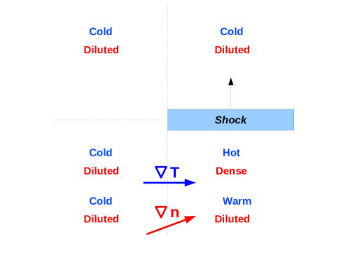
Figure 21: How a finite size shock can generate non-parallel density and temperature (hence pressure) gradients. From [4], p. 406.

$\blacksquare$ But, an equation of state usually gives $p_{e}(n_{e})$. The gradients for $p_{e}$ and $n_{e}$ are thus likely to be parallel, so that the cross product vanishes. How do we break this? Several possibilities,

1. Try a system in rotation around $z$, with $\Omega(z)$. The pressure gradient reads $\nabla P\propto\Omega^{2}(z)\rho(r,\theta)$. It has a $z$ component, while $\nabla\rho(r,\theta)$ has not. Those who’ve read the paper say Biermann considered this option.

2. Try the scheme of Figure 21. Suppose a finite size shock travels through a cold, diluted upstream. The downstream just behind the shock is dense and hot. Far downstream though, the plasma expands but remains warm, so that it is now warm and diluted. The figure shows well how this can generate non-parallel density and temperature (hence pressure) gradients. A non-spherical shock also does the job for similar reasons.

Everything is easily adapted to a system partially ionized. If $n_{n}$ is the density of the neutral, define $\chi=n_{e}/(n_{i}+n_{n})$. Eq. (7) can be adapted dividing the Battery term by $1+\chi$ ([4], p. 406). See [7].

Kulsrud proposed this mechanism to produce Cosmic Fields from scratch in 1997 [5]. Yet, he co-authored in 1992 another paper [6] advocating spontaneous plasmas fluctuations.

Also Khanna [8], showed that a rotating BH in a plasma will always generate toroidal and poloidal magnetic fields.

Ref. [9] studied the Biermann Battery effects in Cosmological MHD Simulations of Population III Star Formation. In its own terms, “We find that the Population III stellar cores formed including this effect are both qualitatively and quantitatively similar to those from hydrodynamics-only (non-MHD) cosmological simulations”. No dynamical effects.

The Biermann battery mechanism was successfully tested in the lab in 2012 [10].

References

[1] L.D. Landau, J. Phys. (U.S.S.R.)10, 25 (1946).
[2] A. Vlasov, J. Phys.9, 25 (1945).
[3] L.D. Landau and E.M. Lifshitz, Course of Theoretical Physics, Physical Kinetic.

References

[1] L.D. Landau, J. Phys. (U.S.S.R.)10, 25 (1946).
[2] L.D. Landau and E.M. Lifshitz, Course of Theoretical Physics, Physical Kinetic.
[3] J.D. Jackson, J. Nucl. Energy, Part C Plasma Phys.1, 171 (1960).
[4] L. Spitzer, Physics of Fully Ionized Gases.
[5] J. Dawson, Phys. Fluids4, 869 (1961).
[6] S. Gayer and C.F. Kennel, Phys. Rev. D19, 1070 (1979)
[17] J.H. Malmberg, C. Wharton, R.W. Gould, and T.M. O’Neil, Phys. Rev. Lett.20, 95 (1968).

References

[1] A. Bret et al., Submitted to Physics of Plasmas, (2012).

References

[1] L. Biermann, Über den Ursprung der Magnetfelder auf Sternen und im interstellaren Raum, Zeitschrift Naturforschung Teil A, 5, 65 (1950).
[2] L. Spitzer, Physics of Fully Ionized Gases.
[3] J.P. Goedbloed and S. Poedts, Principles of Magnetohydrodynamics: With Applications to Laboratory and Astrophysical Plasmas.
[4] R.M. Kulsrud, Plasma Physics for Astrophysics.
[5] R.M. Kulsrud et al., Protogalactic Origin for Cosmic Magnetic Fields, ApJ, 480, 481 (1997).
[6] T. Tajima et al., On the origin of cosmological magnetic fields, ApJ, 390, 309 (1992).
[7] L. Mestel and D.L. Moss, On the Biermann ’battery’ process in uniformly rotating, chemically inhomogeneous stars, MNRAS, 204, 557 (1983).
[8] R. Khanna, Generation of magnetic fields by a gravitomagnetic plasma battery, MNRAS, 295, L6 (1983).
[9] H. Xu et al., The Biermann Battery in Cosmological MHD Simulations of Population III Star Formation, ApJ, 688, L57 (2008).
[10] G. Gregori et al., Generation of scaled protogalactic seed magnetic
fields in laser-produced shock waves, Nature, 481, 480 (2012).