Nonadiabatic generation of coherent phonons

Abstract

The time-dependent density functional theory (TDDFT) is the leading computationally feasible theory to treat excitations by strong electromagnetic fields. Here the theory is applied to coherent optical phonon generation produced by intense laser pulses. We examine the process in the crystalline semimetal antimony (Sb), where nonadiabatic coupling is very important. This material is of particular interest because it exhibits strong phonon coupling and optical phonons of different symmetries can be observed. The TDDFT is able to account for a number of qualitative features of the observed coherent phonons, despite its unsatisfactory performance on reproducing the observed dielectric functions of Sb. A simple dielectric model for nonadiabatic coherent phonon generation is also examined and compared with the TDDFT calculations.

I Introduction

In this paper, we apply time-dependent density functional theory (TDDFT) to calculate coherent phonon generation in crystalline solids. There is fairly clear separation between adiabatic and nonadiabatic regimes for this process, depending on the the material and the frequency of the external electromagnetic field. We first summarize the physical aspects of the phonon generation.

Coherent optical phonons generated by high-intensity, ultrashort laser pulses can be easily observed by pump-probe experiments that are sensitive to the changes in the index of refraction of the probed material. In particular, the phases of the phonons can be extracted from the reflectivity change plotted against the delay time of the reflected probe pulse. These experiments have been done for many kinds of materials. The coupling to optical phonons is especially strong in the semimetals Bi and Sb, and our calculations here will be for crystalline Sb. An example of the kind of data that motivates this choice are shown in Fig. 1 is08 . The pump and the probe pulses are directed on the $[0{\bar{1}}12]$ surface of a Sb crystal at nearly normal incidence. The change in the reflectivity of the probe pulse is measured as a function of the delay between the pump and the probe. One sees an oscillatory pattern whose frequencies can be identified with the known optical phonons in the crystal. The crystal symmetry imposes some conditions between the polarization of the pump pulse and the probe pulse. That information has been used in the experiment to separate the contribution of the $E_{g}$ phonon from that of the $A_{1g}$ phonon. The signal label “isotropic” is due to the $A_{1g}$ phonon while the one labeled “anisotropic” is due to the $E_{g}$ phonon.

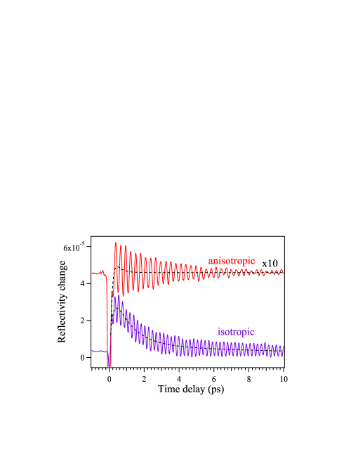
Figure 1: Observation of coherent phonons in crystalline Sb generated by high-intensity laser pulses of 1.55 eV photon energy, from (is08, , Fig. 2a)).

For a given phonon, the reflectivity change is often parameterized by the functional form

$${\Delta R\over R}=ge^{-\Gamma t}\cos(\omega_{ph}t+\phi),$$ (1)

where $g$ is the amplitude, $\omega_{ph}$ is the phonon angular frequency, $\Gamma$ is a damping constant, and $\phi$ is a phase angle. The phase angle $\phi$ provides a very sensitive measure of the mechanism for the phonon generation. If the mechanism is adiabatic, the phase angle should be close to $\pi/2$, as will be discussed below. Typically this is achieved in insulators when the laser photon energy is below the direct band gap. This is called the ”impulsively stimulated Raman scattering” (ISRS) mechanism ya85 , because the entire process can be described in terms of the Raman couplings for exciting a single phonon by a single photon. This process occurs for laser pulses whose duration is shorter than the vibrational frequency. In this mechanism, the coherent phonon coupling depends only on measurable dielectric properties of the medium. The equation of motion in the phonon coordinate is given by a simple formula of Merlinme97 ,

$$\frac{d^{2}q}{dt^{2}}+\omega_{ph}^{2}q=F(t)=\frac{1}{2}\frac{\partial\chi}{\partial q}|{\cal E}(t)|^{2}\,.$$ (2)

Here $q$ is the phonon coordinate, $\chi$ is a component of the dielectric susceptibility tensor, and $\cal E$ is a corresponding component of the electric field.

When real excitations of the medium are possible, another process called the displacive mechanism can contribute as well ze92 ; sc93 ; ku94 . This mechanism takes place in opaque materials like semimetals and in insulators when the laser frequency is above the direct band gap. In the displacive mechanism, the electronic excitations produce a long-term shift in the charge distribution, changing the equilibrium position of the phonon coordinates. Thus the pump pulse produces a state in which the phonon coordinates are displaced from their new equilibrium positions. If the life-time of the excited charges is sufficiently long, the oscillation of the phonons about the new equilibrium will be given by a cosine functional dependence on the time with respect to the pump pulse. Thus, the displacive mechanism has a phase differing by $\pi/2$ with respect to the ISRS mechanism.

At first sight it would seem that the ISRS and the displacive mechanisms are quite different physical processes. In an attempt to establish a unified description, Stevens, Kuhl, and Merlin (SKM) proposed a unified model of to describe both ISRS and displacive mechanisms in term of the dielectric properties of the medium st02 . Their approximate formula for the Fourier component of the force, $F(\Omega)$, is given by,

$$F(\Omega)=C\left[{d{\rm Re}(\varepsilon)\over d\omega}+\frac{2i{\rm Im}(\varepsilon)}{\Omega}\right]\int_{-\infty}^{+\infty}e^{i\Omega t}|E(t)|^{2}dt,$$ (3)

where $E(t)$ is the laser electric field, $\omega$ is the laser frequency, and $\varepsilon$ is the dielectric function. In Sect. IV below we will compare the formula with the results of the TDDFT dynamics to assess the reliability of the approximations made in deriving it.

The transition from adiabatic to nonadiabatic coupling has been observed in crystalline Siha03 ; ri07 ; ka09 as a rather rapid change of phonon phase as the laser photon energy crosses the direct band gap. We have previously applied TDDFT to this system and found that it clearly reproduced this transition sh10 ; note1 . In this work we will use the same computational framework, but applied to a semimetal rather than a semiconductor having a very well defined band gap. However, due to the different crystal symmetry (A7 rather than cubic) the codes had to be significantly modified to treat Sb. In the next section we briefly summarize the computational aspects, in particular the extensions needed for the present application.

II Time-dependent density functional theory

We have found that the Lagrangian formulation of the dynamics problem is very helpful not only from a formal point of view but also to construct the computational equations of motion satisfying the necessary conservation laws. The Lagrangian we used in our earlier study sh10 ; diamond contains the following elements:
1) a fully microscopic treatment for the electron dynamics using a Kohn-Sham (KS) energy functional to evolve the time-dependent electron orbitals;
2) a classical treatment of the time-dependent electric field in the crystalline unit cell;
3) a classical treatment of the dynamics of ionic centers, often called “Ehrenfest dynamics”.

We write the Lagrangian as a sum of three terms, the Kohn-Sham, electromagnetic, and ionic parts.

$$L=L_{KS}+L_{em}+L_{ion}.$$ (4)

The Kohn-Sham term is given the following integral over the unit cell $\Omega$,

$$L_{KS}=\sum_{i}\int_{\Omega}d\vec{r}\left\{\psi_{i}^{*}i\frac{\partial}{\partial t}\psi_{i}-\frac{1}{2m}\left|\left(-i\vec{\nabla}+\frac{e}{c}\vec{A}\right)\psi_{i}\right|^{2}\right\}-\int_{\Omega}d\vec{r}\left\{\left(en_{ion}-en_{e}\right)\phi-E_{xc}[n_{e}]\right\}.$$ (5)

The variables here are the electron orbitals $\psi_{i}({\vec{r}},t)$, the electric field potentials, $\phi({\vec{r}},t)$ and $\vec{A}(t)$, and the ionic coordinates $\vec{R}_{\alpha}(t)$. The vector potential ${\vec{A}}(t)$ is a function of time without spatial dependence and describes spatially-uniform electric field, while a scalar potential $\phi({\vec{r}},t)$ is periodic in the unit cell. The separation of the electric field into these two components is crucial to our computational scheme biry ; ot08 . It enables us to apply Bloch theorem for electron orbitals $\psi_{i}$ at each time. The ionic density $n_{ion}$ is described with the ionic coordinates $R_{\alpha}$ and the electron density $n_{e}$ with the Kohn-Sham orbitals.

We employ the same exchange-correlation energy functional $E_{xc}[n]$ for dynamical calculation as that is used for the ground state calculation. This is the well-known “adiabatic approximation” in time-dependent density functional theory. Of course, the electron dynamics in an external field can be highly non-adiabatic.

The electromagnetic Lagrangian is taken as

$$L_{em}=\frac{1}{8\pi}\int_{\Omega}d\vec{r}\left|\vec{\nabla}\phi\right|^{2}+\frac{\Omega}{8\pi c^{2}}\left(\frac{d\vec{A}}{dt}\right)^{2}.$$ (6)

This form is sufficient to treat the coupling in the medium at length scales small compared to the photon wave length. For the full electrodynamics including the transmission and reflection of photons from the crystal surface, the Lagrangian must also include magnetic fields. This has been carried out in another context, namely the deposition of energy by strong laser pulsesya12 .

We separate the vector potential $\vec{A}(t)$ into external field contribution $\vec{A}_{ext}(t)$ and induced polarization $\vec{A}_{ind}(t)$. Whether to include the induced polarization or not in $\vec{A}(t)$ depends on the macroscopic geometry of the sample and the polarization direction of the electric field. In the present calculation, we employ the longitudinal geometry in which the induced field is included in $\vec{A}(t)$.

Finally, the dynamics in the ion coordinates $\vec{R}_{\alpha}$ is governed by the classical Lagrangian,

$$L_{ion}=\frac{1}{2}\sum_{\alpha}M_{\alpha}\left(\frac{d\vec{R}_{\alpha}}{dt}\right)^{2}+\frac{1}{c}\sum_{\alpha}Z_{\alpha}e\frac{d\vec{R}_{\alpha}}{dt}\vec{A}.$$ (7)

At a formal level, we were able to prove that the TDDFT dynamics reduces to the ISRS formula Eq. (2) in the limit where the laser pulse does not deposit energy into the electronic degrees of freedom. In this adiabatic regime, the relevant dielectric properties can be calculated in perturbation theory based on static density functional theory (DFT), as was done in an early calculation of Raman scattering in Si crystals ba86 . In our full TDDFT calculation in Ref. sh10 , we found that the theory could describe both the adiabatic ISRS and the displacive mechanisms of excitations, thus providing a comprehensive framework for treating coherent laser-lattice interactions.

III Application to Antimony

III.1 Numerical implementation

The solver for the time-dependent Kohn-Sham (KS) equation is a key element for practical computations. Our implementation of the KS solver uses a 3-dimensional real-space grid to represent the orbital wave functions ya96 . This is straightforward for molecules and other finite systems as well as extended materials with cubic crystalline symmetry such as Si. However, Sb has only a rhombic crystal symmetry, and the grid must be modified accordingly. Fortunately, crystals such as the rhombic have a 3-fold symmetry axis, allowing the primitive hexagonal unit cell to be embedded in a supercell having the shape of a rectangular parallelepiped. The construction is shown in Fig. 2. The hexagonal face on the top of the cell is replaced by a rectangle of axes ratio $\sqrt{3}:1$. The Cartesian periodicity needed by the KS solver can then be achieved by changing the mesh spacings in each dimension so that the supercell is spanned by an integer number of mesh points in each direction.

In the case of Sb, the crystal structure is only slightly distorted from cubic, which helps one to construct the lattice as well as to understand the character of the optical phonons. The idealized undistorted lattice is constructed from a simple cubic lattice as shown in Fig. 2. This structure can also be viewed as two interpenetrating face-centered cubic lattices, distinguished in the figure by the red and blue colors of the atoms. The $c$-axis of the cell goes along the $[111]$ direction of the cubes. The length of the $c$-axis in the undistorted geometry is $\sqrt{6}$ larger than the short axis. The actual structure is now obtained by making two transformations. First, the $c$-axis is elongated by a factor of 1.065. Second, one of the cubes is displaced by a small amount (3.3%) along the $c$-axis with respect to the middle of the other cubic. This displacement of the two sublattices with respect to each other define the coordinates of the optical phonons. Displacements along the $c$-axis give rise to the $A_{1g}$ phonon. Displacements perpendicular to the $c$-axis give rise to the doubly-degenerate $E_{g}$ phonon. In a perfectly cubic system all three modes would be degenerate. The offset equilibrium position in the distorted lattice breaks the degeneracy between the frequencies of the $A_{1g}$ and $E_{g}$ phonons, 4.65 THz and 3.47 THz respectively.

For our representation of Sb, the supercell contains 12 atoms and has dimensions $(1,\sqrt{3},\sqrt{6}*1.065)a$ with $a=8.12$ au. We take a mesh of $14\times 30\times 48$ points giving mesh spacings of $(0.58,0.47,0.44)$ au. The solver is described in detail in previous publications. Here we just note that we use a time step of $\Delta t=0.04$ au, which is sufficiently small for the time evolution to be stable. Typically electron orbitals are evolved for 20,000 time steps.

At each time step, the KS wave functions are calculated for a grid of $16^{3}$ $k$-points in the Brillouin zone. The densities for each grid point are summed to obtain an updated KS operator for the next time step. It is convenient to parallelize the code by distributing the calculations for the $k$-points to different processors.

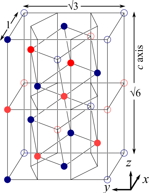
Figure 2: Idealized cubic unit cell illustrating the embedding of the orthorhombic unit cell onto the rectangular supercell. The orthorhombic cell is outlined by the hexagonal prism. Two simple cubes are shown with their $[111]$ axes along the $c$-axis of the supercell. The 12 atoms of the supercell are shown with filled circles. The red and blue atoms define interpenetrating face-centered lattices. The $c$-axis is slightly enlongated to obtain the actual rhombic lattice. In addition, there is a small shift of the red with respect to the blue sublattice along the $c$-axis.

The ionic motion is very small during the time of passage of the pump pulse, and we don’t attempt to solve Newton’s equations directly within the time-dependent evolution of the system. As in Ref. sh10 , the code only calculates the force on the ions. This is later decomposed a transient part and a constant part in the final state for the final analysis.

The energy functional in our calculations treats explicitly the 5 electrons in the $(5s)^{2}(5p)^{3}$ atomic orbitals. The interaction with the ionic cores is taken as the Troullier-Martins tr91 pseudopotential with the range of the nonlocality of 4.0 au. The electron-electron interaction is treated in the local density approximation using the standard parameterization pz81 .

III.2 Calculated electronic structure

The group V elements, As, Sb, and Bi, have a complicated band structure due their rhombohedral A7 crystalline symmetry. They are distinguished by a small but nonzero overlap between nominally valence and conduction bands. This gives the crystal the characteristics of a semimetal, namely a conductor with a very small carrier density. There are several DFT calculations of the electronic structure which reproduce this important featurego90 ; sh99 . For example, the calculation of Ref. go90 found a carrier density of $2.3\times 10^{-3}$ electrons per atom in Sb compared to the experimental value of $1.1\times 10^{-3}$. Our DFT calculation gives a similar density of electron states and a carrier density of $2.4\times 10^{-3}$ electrons per atom. In any case, details of the density of states within a few tenths of eV of the Fermi level should not be crucial to the dynamics at the much higher energy of the laser photon.

Beyond the static electronic structure, it is important to establish the accuracy of the linear response predictions if the dynamic electronic properties are the object of the calculations. There do not seem to be any DFT calculations of the dielectric properties in the literature, so we describe our results in some detail in the Appendix. Unfortunately, our predicted dielectric properties do not agree well with the evaluated measurements pa98 . However, the evaluated dielectric function is derived from the measured reflectivity function which seems to depend significantly on temperature. In fact our predicted reflectivity agrees fairly well with the data at 77K but not with room temperature data. Since that experimental finding seems not to be understood up to now, we cannot draw any strong conclusions about the origin of the disagreement with theory. In any case, our TDDFT results can be compared with the simple models to evaluate the reliability of the approximations made in the models.

III.3 Typical results

In this section, we show the results of the time-dependent calculations for typical conditions. As shown in Fig. 2, we set the $z$-axis in our calculation parallel to the $c$-axis. The form of the external electric field is chosen as

$$\vec{\cal E}_{ext}(t)=\hat{x}{\cal E}_{0}\sin(\pi t/T)\sin(\omega t),$$ (8)

where the polarization direction is chosen along the $x$-axis, ${\cal E}_{0}$ is the maximum value of the electric field, $\omega$ is the laser frequency, and $T$ is the pulse duration. Crystal symmetry permits this field to excite the $A_{1g}$ mode and the $x$ component of the $E_{g}$ mode.

As we mentioned in Sec. II, we include the induced polarization field in the vector potential $\vec{A}(t)$. For a sufficiently weak electric field, the external and the total (external + induced) electric fields are related to each other by the dielectric function,

$${\cal E}_{tot}(t)=\int^{t}\varepsilon^{-1}(t-t^{\prime}){\cal E}_{ext}(t^{\prime})dt^{\prime}.$$ (9)

The external and total fields for a typical run are shown in Fig. 3. Here the parameters for the external field are taken as $\hbar\omega=1.6$ eV, $T=16$ fs, and ${\cal E}_{0}$ corresponding to an intensity of $10^{13}$ W/cm².

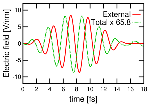
Figure 3: External and screened electric fields in the Sb crystal. See text for explanation.

We see that the total field is almost out of phase to the external field and about 66 times smaller in amplitude. The ratio and the phase between the two corresponds well to the calculated dielectric function at $\omega=1.6$ eV/${\hbar}$, shown in Fig. 9, even though the dielectric function is only strictly valid in the small amplitude regime.

The electron density in two planes through the unit cell are shown in Fig. 4. In panel (a), the atomic positions in the rectangular supercell are depicted with the actual distortion of the cubic lattice into rhombohedral. The electron densities are shown in panels (b)-(d) on planes indicated by green-solid and purple-dashed frames. The green-solid frame is the $xz$-plane through the middle of the unit cell. This plane includes the polarization direction of the electric field as well as the $c$-axis of the crystal. The purple-dashed frame is obtained by rotating the $xz$-plane by 120^∘ around the $c$-axis passing through the central atom.

The ground-state electron density, shown in (b), is the same in the two planes. Each atom has three bonds with nearest neighbors and one of the bonds lies within each plane. Among five valence electrons, three of them are associated with the bonds and two of them occupy lone-pair orbitals.

The particle-hole excitation changes the occupation probabilities in the final state, affecting the electron density distribution. This is shown in two panels, (c) and (d). The panel (c) shows the change of electron density from that in the ground state in the $zx$ plane of the green-solid frame in (a). The orange color indicates increase of the electron density from the grand state, while the blue color indicates decrease. The panel (d) shows the change of electron density in the plane of purple-dashed frame in (a).

There are two spatial regions where electron density changes most from that in the ground state. One is the excitation from lone-pair orbitals. This corresponds to the region just above and below the positions of atoms indicated as A in (c). This change is seen both in (c) and (d). The other is the excitation out of the bonding orbitals, causing a decrease of the density around the midpoint of the bonds. This removal of bonding electrons is seen clearly in (c) in the areas indicated as B in (c). The effect is much smaller in (d) because the electric field vector is not in the plane of the that bond. We also note that increase of electrons density is seen in the area C in (c), not in (d). These anisotropic changes of electron density certainly contribute to the force on the optical phonon modes, which we now discuss.

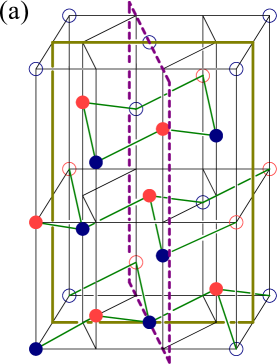
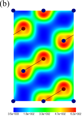
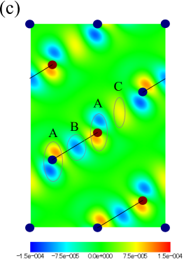
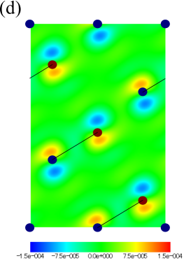
Figure 4: (a) Atomic positions in the rectangular unit cell. An $xz$-plane through the middle of the cell is framed in a solid green rectangle. The purple-dashed frame marks the plane obtained by rotating green-solid frame by 120^∘ around the $c$-axis. (b) The ground state electron density on the two planes. (c) Density change in the final state on the $xz$ plane (green-solid frame). (d) Density change on the rotated plane (purple-dashed frame).

The next two figures show the force on the phonon modes for the external field of Fig. 3. In Fig. 5, the external field is in the $x$ direction. The $E_{g}$ phonon excitation will then also be in the $x$ direction; the $A_{1g}$ phonon is always along the $z$ axis. The oscillatory part of the force may be associated with the ISRS excitation mechanism. The force reaches a constant plateau at the end of the pulse; its plateau value controls the strength of the displacive mechanism. Note that the $A_{1g}$ mode is much stronger than the $E_{g}$ mode. This agrees with the experimental measurements, which always see a larger effect for the $a_{1g}$ mode.

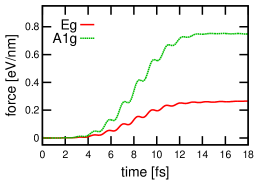
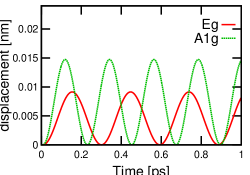
Figure 5: a) Force on phonon modes excited by the external field in the $x$-direction. b) corresponding displacement of phonon coordinates.

Fig. 6 shows the forces resulting from the same external field but oriented along the $z$ axis. The strength of the $A_{1g}$ force is about the same as in the other orientation, but now the $E_{g}$ force vanishes. This is consequence of the crystal symmetry.

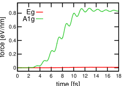
Figure 6: Force on phonon modes excited by the external field in the $z$-direction.

In panel b) of Fig. 5, we integrate the equation of motion for the phonon mode to find the displacement as a function of time. Since the force is constant in the final state, the displacement function will be close to the form $1-\cos(\omega_{ph}(t-t_{0}))$ where $t_{0}$ is near the maximum amplitude point of the driving field. Thus the phonon will have a displacive phase. In fact we find that the displacive mechanism dominates for all external field frequencies in the range of 1.0-3.0 eV/$\hbar$.

We now turn to the phase of the coherent phonon. The displacive mechanism dominates for both modes in the TDDFT calculation, as is clear from the force plateaus in Fig. 5 and 6. The experiments reported in Refs. ga96 ; is08 obtain a phase consistent with the displacive mechanism for the $A_{1g}$, in agreement with the TDDFT. However, they find a difference in phase for the $E_{g}$ mode, which is not explained by the theory. One possible origin of the phase differences could be differences in relaxation times of excited carriers responsible for two mode. Unfortunately, the electronic relaxation in the final state is beyond the scope of the TDDFT.

IV Comparison with the SKM model

In Ref. st02 , Stevens, Kuhl, and Merlin proposed a dielectric model for the force acting on phonon mode. Taking Fourier transform of Eq. (3), we may obtain the force as a function of time,

$$F(t)=C\left[\frac{d{\rm Re}(\varepsilon)}{d\omega}|E(t)|^{2}+2{\rm Im}(\varepsilon)\int^{t}_{-\infty}dt^{\prime}|E(t^{\prime})|^{2}\right].$$ (10)

This formula indicates that the real part of $\varepsilon$ is related to the impulsive force, $F(t)\sim|E(t)|^{2}$, corresponding to the ISRS mechanism, while the imaginary part of $\varepsilon$ gives a constant force at $t\rightarrow+\infty$ corresponding to the displacive mechanism. In this section, we will make a theory-to-theory comparison of this equation within the TDDFT dynamics. We compare the force at $t\rightarrow+\infty$ as a function of laser frequency with the imaginary part of the dielectric function, and examine the validity of the dielectric model.

Figure 7 show the plateau values of the force at $t\rightarrow+\infty$. In this figure, the intensity of the external electric field is taken to be the same. However, the electric field in Eq. (10) is the actual electric field in the medium. We take this into account by scaling our calculated force by $|\varepsilon(\omega)|^{2}$ to compare with the imaginary part of the dielectric function.

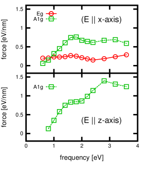
Figure 7: Forces in the final state as a function of the field frequency.

In Fig. 8, we show the forces multiplied with $|\varepsilon(\omega)|^{2}$. The top panel shows the results for the electric field in the $x$-direction. The force calculated in TDDFT is shown as green squares and red circles. The bottom panel shows the quantities for the electric field in the $z$-direction. The $E_{g}$ force vanishes by symmetry and is not shown. We find the forces as a function of frequency exhibit different behavior depending on phonon modes and polarization of electric field.

We test the SKM model by comparing the forces with the imaginary part of the dielectric function which is shown in the Appendix. In the top panel, the imaginary part of the dielectric function in $x$-direction, ${\rm Im}\varepsilon_{xx}$, normalized to reproduce the magnitude of the $E_{g}$ force (red circles) is shown. One sees that the model reproduces the frequency dependence of the $E_{g}$ force quite well. In the bottom panel, ${\rm Im}\varepsilon_{zz}$ normalized to reproduce the magnitude of the $A_{1g}$ force (green squares) is shown. The model again reproduces the trend of the $A_{1g}$ force quite well. In both cases, the model describes the variation in a force when the phonon coordinates are parallel to the electric field. However, for the $A_{1g}$ force in the top panel, the force along $z$-direction in the $x$ polarization direction, the frequency dependence does not resemble either ${\rm Im}\varepsilon_{xx}$ or ${\rm Im}\varepsilon_{zz}$.

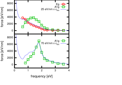
Figure 8: Comparison of forces calculated by the TDDFT compared to the SKM model. a) electric field in the $x$ direction; b) electric field in the $z$ direction.

V Conclusions and outlook

The TDDFT has given us a calculational framework to study the transition from adiabatic to nonadiabatic processes in extended systems. In previous work, we found that an important qualitative aspects of the transition, namely the phase of the coherently generated phonon, was correctly reproduced by the theory in crystalline silicon. In this work, we have applied the same methodology to a more challenging material, namely the semimetal antimony. The noncubic symmetry presents some computational problems that have been overcome. The optical phonons have a more rich spectroscopy than in the cubic systems, and there are symmetry-dictated dependencies that are reproduced by the theory. Unfortunately, the present theory is not accurate enough at the linear response level to give quantitative predictions for the coherent phonon generation. At a qualitative level, the theory predicts a nonadiabatic response over a wide range of frequencies. At the experimentally measured frequency, the $A_{1g}$ mode shows the nonadiabatic behavior but the observed phase of the $E_{g}$ mode is different.

This study points out the need for a more accurate theory of the electronic structure of Sb. It might be that the $sp$ space is too restrictive; there is a closed $d$ shell close to the Fermi energy that could be easily polarized. Also, the theory needs to be developed to treating the transmission and reflection of the electromagnetic pulses from the interfaces of the media, in order to describe the measurements quantitatively.

Appendix: Dielectric properties of Sb

It is important to check how well the TDDFT performs in the linear response region, if one wishes to extend the domain to nonlinear processes. To that end, we first calculate the dielectric properties using the TDDFT and following the real-time method proposed in Ref. biry . There are two independent components of the dielectric tensor in crystals of A7 symmetry, $\varepsilon_{xx}$ and $\varepsilon_{zz}$ in our coordinate system. They are shown in Fig. 9. In the low frequency limit, the real parts are dominated by the free carriers and go to negative infinity. At intermediate frequencies the real part is very anisotropic but becomes isotropic above 2 eV. The imaginary part is also very anisotropic in the energy range below 3 eV.

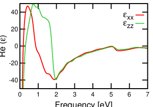
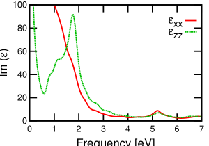
Figure 9: Calculated dielectric tensor $\varepsilon(\omega)$, real-part in the left and imaginary-part in the right panels. Red: $xx$ component; blue: $zz$ component.

The compilation pa98 of evaluated experimental dielectric functions has a table of $\varepsilon_{xx}$ for Sb, which we compare with in Fig. 10. In both theory and experiment, one sees large absorption strength at low frequencies tapering off smoothly as the frequency increases. However, the agreement is not good at a quantitatively level, unlike the situation in simple cubic materials. The theory is also disappointing for describing the real part of $\varepsilon_{xx}$.

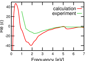
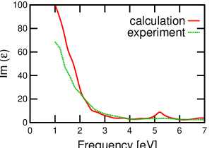
Figure 10: Calculated $\varepsilon_{xx}$ compared with evaluated data of Ref. pa98 . Real-part in the left and imaginary-part in the right panels, respectively.

In an attempt to get some insight into possible origins of the disagreement, we went back to the actual reflectivity data ca64 that were used to obtain the dielectric function. This data has an unexplained temperature dependence with a significantly higher reflectivity at 77 K. The theoretical reflectivity, $R$, is easily evaluated as

$$R=\left|{\varepsilon^{1/2}-1\over\varepsilon^{1/2}+1}\right|.$$ (11)

The comparison between experimental and theoretical $R$ is shown in Fig. 11. The theory clearly disagrees with the room-temperature data. However, it reproduces rather well the low temperature data up to about 5 eV photon energy. Whether this is a pure accident or suggests some missing physics we cannot say.

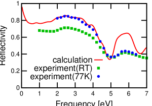
Figure 11: Calculated reflectivity of Sb compared with experiment ca64 . Line: theory; solid squares: room temperature data; solid circles: data at 77K.

References

- (1) K. Ishioka, M. Kitajima, and O. Misochko, J. Appl. Phys. 103, 123505 (2008).
- (2) Y.-X. Yan, E.B. Gamble, Jr., and K.A. Nelson, J. Chem. Phys. 83, 5391 A(1985B).
- (3) R. Merlin, Solid State Commun. 102, 207 (1997).
- (4) H.J. Zeiger, J. Vidal, T.K. Cheng, E.P. Ippen, G. Dresselhaus, and M.S. Dresselhaus, Phys. Rev. B45, 768 (1992).
- (5) R. Scholz, T. Pfeifer and H. Kurz, Phys. Rev. B47, 16229 (1993).
- (6) A.V. Kuznetsov and C.J. Stanton, Phys. Rev. Lett. 73, 3243 (1994).
- (7) T.E. Stevens, J. Kuhl and R. Merlin, Phys. Rev. B65, 144304 (2002).
- (8) M. Hase, M. Kitajima, A. Constantinescu, and H. Petek, Nature 426, 51 (2003).
- (9) D.M. Riffe and A.J. Sabbah, Phys. Rev. B76, 085207 (2007).
- (10) K. Kato, A. Ishizawa, K. Oguri, K. Tateno, T. Tawara, H. Gotoh, M. Kitajima, H. Nakano, Japanese J. Appl. Phys. 48, 100205 (2009).
- (11) Y. Shinohara, K. Yabana, Y. Kawashita, J.-I. Iwata, T. Otobe, and G.F. Bertsch, Phys. Rev. B 82, 155110 (2010).
- (12) While the rapid change around the direct gap is reproduced by TDDFT, the energy of the direct gap is typically predicted too low in the underlying DFT theory.
- (13) Y. Shinohara, Y. Kawashita, J.-i. Iwata, K. Yabana, T. Otobe, and G.F..Bertsch, J. Phys. Cond. Matter 22, 384212 (2010)..
- (14) G.F. Bertsch, J.-I. Iwata, A. Rubio, and K. Yabana, Phys. Rev. B62, 7998 (2000).
- (15) T. Otobe, M. Yamagiwa, J.-I. Iwata, K. Yabana, T. Nakatsukasa, and G.F. Bertsch, Phys. Rev. B77, 165104 (2008).
- (16) K. Yabana, T. Sugiyama, Y. Shinohara, T. Otobe, and G.F. Bertsch, Phys. Rev. B 85, 045134 (2012).
- (17) S. Baroni and R. Resta, Phys. Rev. B33, 5969 (1986).
- (18) K. Yabana and G.F. Bertsch, Phys. Rev. B54, 4484 (1996).
- (19) N. Troullier and J.L. Martins, Phys. Rev. B 43, 1993 (1991).
- (20) J.P. Perdew and A. Zunger, Phys. Rev. B23, 5048 (1981).
- (21) X. Gonze, J.-P. Michenaud, and J.-P. Vigneron,, Phys. Rev. B 41, 11827 (1990).
- (22) A.B. Shick, J.B. Ketterson, D.L. Novikov, and A.J. Freeman, Phys. Rev. B60, 15484 (1999).
- (23) D. Lynch and W. Hunter, Handbook of Optical Constants of Solids III, ed. E. Palik, (Academic Press, New York, 1998), p. 277-278.
- (24) G.A. Garrett, T.F. Albrecht, J.F. Whitaker, and R. Merlin, Phys. Rev. Lett. 77, 3661 (1996).
- (25) M. Cardona and D.L. Greenaway, Phys. Rev. 133, A1685 (1964).