Quantum field theoretic approach to neutrino oscillations in matter

Abstract

We consider neutrino oscillations in non-uniform matter in a quantum field theoretic (QFT) approach, in which neutrino production, propagation and detection are considered as a single process. We find the conditions under which the oscillation probability can be sensibly defined and demonstrate how the properly normalized oscillation probability can be obtained in the QFT framework. We derive the evolution equation for the oscillation amplitude and discuss the conditions under which it reduces to the standard Schrödinger-like evolution equation. It is shown that, contrary to the common usage, the Schrödinger-like evolution equation is not applicable in certain cases, such as oscillations of neutrinos produced in decays of free pions provided that sterile neutrinos with $\Delta m^{2}\gtrsim 1$ eV² exist.

1 Introduction

In experiments with solar, atmospheric and supernova neutrinos, the neutrinos propagate significant distances in matter before reaching detectors; the same will also be true for the proposed very long baseline accelerator neutrino experiments. Matter can affect neutrino oscillations drastically, leading, in particular, to their resonance enhancement through the Mikheyev-Smirnov-Wolfenstein (MSW) effect Wolf ; MS or through the parametric enhancement mechanism param . It is thus extremely important to put the analyses of neutrino oscillations in matter on a solid theoretical basis.

The standard approach to neutrino oscillations in matter, pioneered by Wolfenstein Wolf , is as follows. Mass eigenstate neutrinos $\nu_{i}$, composing a given flavour neutrino state $\nu_{\alpha}$, are assumed to have the same momentum (and, due to their different mass, different energies). In the case of oscillations of relativistic neutrinos in vacuum, the evolution of the transition amplitude in the flavour basis is then described by the Schrödinger equation

$$i\frac{d}{dt}|\nu\rangle=H_{0}\,|\nu\rangle\,,\qquad~{}~{}H_{0}=U\!\left[p\cdot\!{\mathbbm{1}}+\frac{M_{d}^{2}}{2p}\right]\!U^{\dagger}\,.$$ (1)

Here $|\nu\rangle=(|\nu_{e}\rangle,\,|\nu_{\mu}\rangle,\,|\nu_{\tau},\rangle\,...)^{T}$ is the flavour-basis neutrino state vector (with dots standing for possible light sterile neutrino states), $p$ is the neutrino momentum, $M_{d}={\rm diag}(m_{1},\,m_{2},\,m_{3},\,...)$ is the neutrino mass matrix in the mass eigenstate basis, and $U$ is the leptonic mixing matrix which relates the flavour-eigenstate neutrino state vectors $|\nu_{\alpha}\rangle$ ($\alpha=e,\mu,\tau,\dots$) with the mass-eigenstate ones $|\nu_{i}\rangle$ ($i=1,2,3,...)$:

$$|\nu_{\alpha}\rangle=\sum_{i}U^{*}_{\alpha i}|\nu_{i}\rangle\,.$$ (2)

Since the first term in the square brackets in the expression for $H_{0}$ in (1) is proportional to the unit matrix, it leads to a common phase shift of all neutrino flavour states and therefore does not affect the oscillation probabilities. Thus, it can be omitted from $H_{0}$. The matter effects on neutrino oscillations can be incorporated by replacing the free Hamiltonian $H_{0}$ by the effective Hamiltonian of neutrino propagation in matter according to $H_{0}\to H=H_{0}+V$. Here $V$ is the matrix of matter-induced neutrino potentials due to coherent forward scattering of neutrinos on matter constituents; in the absence of background neutrinos it is diagonal in the flavour-eigenstate basis. Taking into account that for pointlike relativistic neutrinos the distance $x$ they propagate over the time $t$ satisfies $x\simeq t$ and that to leading order in small neutrino masses $p\simeq E$ where $E$ is the average neutrino energy, one arrives at the following equation describing neutrino flavour evolution in matter:

$$i\frac{d}{dx}|\nu\rangle=\left[U\frac{M_{d}^{2}}{2E}U^{\dagger}+V(x)\right]|\nu\rangle\,.$$ (3)

Equation (3) is employed in virtually all studies of neutrino oscillations in non-uniform matter. However, its derivation presented above was based on heuristic considerations and it certainly needs to be put on a more solid ground. Attempts at deriving eq. (3) within the relativistic quantum mechanics and quantum field theory (QFT) frameworks have been made in a number of papers. In Halprin evolution of Dirac neutrinos in matter was described by making use of a Dirac equation with matter-induced potential. It was demonstrated that the neutrino wave function satisfies eq. (3) provided that matter density varies little over the distances of order of the neutrino de Broglie wavelength. The Dirac equation was also employed in changzia , though only the case of matter of constant density was considered there. In ref. mannheim the Dirac equation was used to describe the evolution of Dirac and Majorana neutrinos in matter, but again only in the case of constant-density matter. Besides the already mentioned ref. Halprin , the Dirac equation has been employed for describing neutrino oscillations in non-uniform matter in refs. sawyer ; grimus , both in the Dirac sawyer ; grimus and Majorana grimus neutrino cases. In none of these papers, however, neutrino production and detection processes were included in the description of neutrino oscillations. The most advanced study of neutrino evolution in matter of varying density was carried out in cardchung in the QFT framework. In that paper the treatment included the neutrino production and detection processes, and it was also demonstrated how the correctly normalized oscillation probability can be obtained. The employed normalization procedure was rather cumbersome, though.

The main goal of refs. [4-9] was to derive the evolution equation (3) from relativistic quantum mechanics or QFT. However, the conditions under which this equation is valid were not fully studied in those papers. Furthermore, the question of how neutrino oscillations can be described in the situations when these conditions are not satisfied (and consequently eq. (3) cannot be used) was not addressed. In addition, no discussion of neutrino production and detection coherence and of their effect on neutrino oscillations in matter was given.

In the present paper we consider neutrino oscillations in non-uniform matter in the framework of QFT. In this approach neutrino production, propagation, and detection are treated as a single process, described by a Feynman diagram with the neutrino in the intermediate state (such as the one in fig. 1). We discuss the conditions under which the oscillation probability can be extracted from the rate of the overall neutrino production-propagation-detection process and demonstrate that this probability is automatically correctly normalized and satisfies the unitarity constraints. We also identify the conditions under which the amplitude of neutrino flavour transition can be found as a solution of eq. (3). One of our main results is that eq. (3) is not applicable when neutrino production and/or detection coherence is violated. We discuss the situations when this can happen and consider an alternative way of describing neutrino oscillations in those cases.

Our treatment of neutrino oscillations in non-uniform matter closely parallels the treatment of neutrino oscillations in vacuum performed in ref. AK , but differs from the latter in a number of important aspects. The differences are mostly related to the properties of the neutrino propagator in non-uniform matter, which deviate significantly from those of the vacuum neutrino propagator and do not allow using some techniques that were applied to the neutrino propagator in vacuum. To make it easier to follow our treatment, let us briefly outline our main steps.

• We consider the neutrino production, propagation and detection process described by the Feynman diagram of fig. 1. The external legs in this diagram correspond to the particles that accompany neutrino production and detection. These are either propagating particles or bound states, which are described by the suitable state vectors. The intermediate neutrino state is described by a propagator, which is found as a solution of the corresponding Dirac equation with matter-induced potential for neutrinos $V({\mathbf{x}})$.

• Since this potential depends on the coordinate ${\mathbf{x}}$, the system is not translationally invariant and the neutrino momentum is not conserved. As a result, the neutrino propagator in the momentum space depends on two momenta, ${\mathbf{p}}$ and ${\mathbf{p}}^{\prime}$, rather than one. The amplitude of the overall process can be written as the integral over these two momenta, with the production and detection amplitudes $\Phi_{P}({\mathbf{p}})$ and $\Phi_{D}({\mathbf{p}}^{\prime})$ multiplying the momentum-space neutrino propagator $\tilde{S}(E;{\mathbf{p^{\prime}}},{\mathbf{p}})$ in the integrand.

• For the intervals of momenta over which the propagator varies significantly, the neutrino production and detection amplitudes $\Phi_{P}({\mathbf{p}})$ and $\Phi_{D}({\mathbf{p}}^{\prime})$ change very little. This allows one to greatly simplify the expression for the amplitude of the process.

• We calculate the rate of the overall neutrino production-propagation-detection process and identify the conditions under which this rate factorizes into the neutrino production rate $d\Gamma_{\alpha}^{prod}/dE$, propagation (oscillation) probability $P_{\alpha\beta}$ and the detection cross section $\sigma_{\beta}$. When these conditions are satisfied, the oscillation probability can be extracted from the rate of the overall process by dividing the latter by $d\Gamma_{\alpha}^{prod}/dE$ and $\sigma_{\beta}$.

• We reconstruct the oscillation amplitude from the expression for $P_{\alpha\beta}$ and derive the equation that it obeys. We identify the conditions under which this equation coincides with eq. (3) and also discuss the situations when these conditions are violated and eq. (3) is not applicable.

The described above program is realized in sections 2-4 of the paper; in section 5 we summarize and discuss the obtained results. To make the paper self-contained, in Appendix A we briefly review the derivation of the neutrino propagator in non-uniform matter performed in cardchung , whereas in Appendix B we give a compendium of expressions for neutrino potentials in matter. Appendices C and D contain derivation of some results used in sections 2.2 and 4.

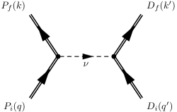
Figure 1: Feynman diagram describing neutrino production, propagation and detection as a single process.

2 The transition amplitude

2.1 General formalism

Consider the process of neutrino production, propagation and detection described by the Feynman diagram of fig. 1. We shall be assuming that the neutrino production process involves one initial state and one final state particle (besides the neutrino). Likewise, the detection process will also be assumed to involve only one particle besides the neutrino in the initial state and one particle in the final state. The generalization to the case of an arbitrary number of particles involved in the neutrino production and detection processes is straightforward and would just make the formalism more cumbersome without providing further physical insight.

Let us first discuss the state vectors of the particles accompanying neutrino production and detection (external particles). In quantum theory, one-particle states of particles of type $A$ can be written as

$$|A\rangle=\int\![dp]\,f_{A}({\mathbf{p}},{\mathbf{P}})\,|A,{\mathbf{p}}\rangle\,,$$ (4)

where $|A,{\mathbf{p}}\rangle$ is the one-particle momentum eigenstate corresponding to momentum ${\mathbf{p}}$ and energy $E_{A}({\mathbf{p}})$, and $f_{A}({\mathbf{p}},{\mathbf{P}})$ is the momentum distribution function with the mean momentum ${\mathbf{P}}$. In eq. (4) we use the shorthand notation

$$[dp]\equiv\frac{d^{3}p}{(2\pi)^{3}\sqrt{2E_{A}({\mathbf{p}})}}\,.$$ (5)

For particles with spin, the states $|A\rangle$ and $|A,{\mathbf{p}}\rangle$ depend also on a spin variable, which we suppress to simplify the notation.

Throughout this paper we will be using the normalization conventions of ref. PeskSchr and the notation $P_{L,R}=(1\mp\gamma_{5})/2$. We choose the Lorentz invariant normalization condition for the plane wave states $|A,{\mathbf{p}}\rangle$:

$$\langle A,{\mathbf{p}}^{\prime}|A,{\mathbf{p}}\rangle=2E_{A}({\mathbf{p}})\,(2\pi)^{3}\delta^{(3)}({\mathbf{p}}-{\mathbf{p^{\prime}}})\,.$$ (6)

The standard normalization of the states $\langle A|A\rangle=1$ then implies

$$\int\!\frac{d^{3}p}{(2\pi)^{3}}\,|f_{A}({\mathbf{p}})|^{2}=1\,.$$ (7)

The states describing the external particles in fig. 1 can be represented in the form (4). For the initial and final states at neutrino production we write

$$|P_{i}\rangle=\int\![dq]\,f_{Pi}({\mathbf{q}},{\mathbf{Q}})\,|P_{i},{\mathbf{q}}\rangle\,,\qquad|P_{f}\rangle=\int\![dk]\,f_{Pf}({\mathbf{k}},{\mathbf{K}})\,|P_{f},{\mathbf{k}}\rangle\,,$$ (8)

and similarly for the states participating in neutrino detection:

$$|D_{i}\rangle=\int\![dq^{\prime}]\,f_{Di}({\mathbf{q}}^{\prime},{\mathbf{Q}}^{\prime})\,|D_{i},{\mathbf{q}}^{\prime}\rangle\,,\qquad|D_{f}\rangle=\int\![dk^{\prime}]\,f_{Df}({\mathbf{k}}^{\prime},{\mathbf{K}}^{\prime})\,|D_{f},{\mathbf{k}}^{\prime}\rangle\,.$$ (9)

We assume these states to obey the normalization condition (7). Some (or all) of the mean momenta of the external particles ${\mathbf{Q}}$, ${\mathbf{K}}$, ${\mathbf{Q}}^{\prime}$ and ${\mathbf{K}}^{\prime}$ may vanish, i.e. the states in eqs. (8) and (9) can describe bound states at rest as well as wave packets.

The amplitude of the neutrino production - propagation - detection process is given by the matrix element

$$i{\cal A}_{\beta\alpha}=\langle P_{f}\,D_{f}|\hat{T}\exp\Big{[}-i\int\!d^{4}x\,{\cal H}_{I}(x)\Big{]}-\mathbbm{1}|P_{i}\,D_{i}\rangle\,,$$ (10)

where $\hat{T}$ is the time ordering operator and ${\cal H}_{I}(x)$ is the charged-current weak interaction Hamiltonian. From this equation it is easy to calculate the transition amplitude in the lowest nontrivial order in ${\cal H}_{I}$ using the standard QFT methods. The resulting expression corresponds to the Feynman diagram of fig. 1 and can be written as

$$i{\cal A}_{\beta\alpha} = \int\![dq]\,f_{Pi}({\mathbf{q}},{\mathbf{Q}})\int\![dk]\,f^{*}_{Pf}({\mathbf{k}},{\mathbf{K}})$$ (11)

$$\times\int\![dq^{\prime}]\,f_{Di}({\mathbf{q}}^{\prime},{\mathbf{Q}}^{\prime})\int\![dk^{\prime}]\,f^{*}_{Df}({\mathbf{k}}^{\prime},{\mathbf{K}}^{\prime})\,i{\cal A}^{p.w.}_{\beta\alpha}(q,k;q^{\prime},k^{\prime})\,.$$

Here the quantity ${\cal A}^{p.w.}_{\beta\alpha}(q,k;q^{\prime},k^{\prime})$ is the amplitude of the process with plane-wave external states:

$$i{\cal A}^{p.w.}_{\beta\alpha}(q,k;q^{\prime},k^{\prime})=\int d^{4}x_{1}\!\int d^{4}x_{2}\, \tilde{M}_{D}(q^{\prime},k^{\prime})\,e^{-i(q^{\prime}-k^{\prime})(x_{2}-x_{D})}$$

$$\times S_{\beta\alpha}(x_{2},x_{1})\tilde{M}_{P}(q,k)\,e^{-i(q-k)(x_{1}-x_{P})}\,.\qquad$$ (12)

In this equation $x_{1}$ and $x_{2}$ are the 4-coordinates of the neutrino production and detection points. The choice of the 4-coordinate dependent phase factors corresponds to the assumption that the peaks of the wave packets of particles involved in the production process are all located at ${\mathbf{x}}_{1}={\mathbf{x}}_{P}$ at the time $t_{1}=t_{P}$, whereas for the detection process the corresponding peaks are all situated at ${\mathbf{x}}_{2}={\mathbf{x}}_{D}$ at the time $t_{2}=t_{D}$ (this assumption can be relaxed, see section 6.2 of ref. AK ). The quantities $\tilde{M}_{P}(q,k)$ and $\tilde{M}_{D}(q^{\prime},k^{\prime})$ are the plane-wave amplitudes of the processes $P_{i}\to P_{f}+\nu_{\alpha}$ and $D_{i}+\nu_{\beta}\to D_{f}$, respectively, with the neutrino spinors excluded. They are related to the full plane-wave neutrino production and detection amplitudes $M_{P}(q,k)$ and $M_{D}(q^{\prime},k^{\prime})$ through

$$M_{P}(q,k)=\frac{\bar{u}_{L}(p)}{\sqrt{2p_{0}}}\tilde{M}_{P}(q,k)\,\qquad\mbox{and}\qquad M_{D}(q^{\prime},k^{\prime})=\tilde{M}_{D}(q^{\prime},k^{\prime})\frac{u_{L}(p^{\prime})}{\sqrt{2p_{0}^{\prime}}}\,.$$ (13)

Here $u_{L}(p)$ is the left-handed neutrino spinor, $p=q-k$, $p^{\prime}=q^{\prime}-k^{\prime}$, and $p_{0},\,p_{0}^{\prime}$ are the time components of the corresponding 4-momenta.

The quantity $S_{\beta\alpha}(x_{2},x_{1})$ in the second line of eq. (12) is the coordinate-space neutrino propagator in matter in the flavour basis. It is a matrix in both flavour space and spinor space, whereas the quantities $\tilde{M}_{P}(q,k)$ and $\tilde{M}_{D}(q^{\prime},k^{\prime})$ are Dirac spinors. To simplify the notation, we have suppressed the corresponding spinor indices.

The neutrino propagator in matter $S_{\beta\alpha}(x,x^{\prime})$ satisfies the Schwinger-Dyson equation

$$[i\gamma_{\mu}\partial^{\mu}-MP_{R}-M^{\dagger}P_{L}]S(x,x^{\prime})-\int d^{4}x^{\prime\prime}\,\Sigma(x,x^{\prime\prime})PS(x^{\prime\prime},x^{\prime})=\delta^{4}(x-x^{\prime})\!\cdot\!\mathbbm{1}\,,$$ (14)

where $M$ is the neutrino mass matrix in the flavour basis, $\Sigma(x,x^{\prime})$ is the matter-induced neutrino self-energy, $\mathbbm{1}$ is the unit matrix in the flavour space, and flavour indices are suppressed for simplicity. Eq. (14) (as well as eq. (16) below) applies to both Dirac and Majorana neutrino cases, provided that for Majorana neutrinos one uses the Feynman rules with propagators and vertices not containing explicitly the charge-conjugation matrix (see, e.g., gates ; denner ). The operator $P$ in (14) is defined as $P=P_{L}$ for Dirac neutrinos and $P=-\gamma_{5}$ for Majorana neutrinos. We will discuss the choice of the operator $P$ in the Majorana neutrino case in Appendix A.

For Dirac neutrinos, the mass matrix $M$ is a general $N_{f}\times N_{f}$ matrix where $N_{f}$ is the number of light neutrino species. Note that for $M\neq M^{\dagger}$ the presence of the term $MP_{R}+M^{\dagger}P_{L}$ rather than the usual mass term $M$ in (14) is required by the hermiticity of the Lagrangian. For Majorana neutrinos, $M=M^{T}$.

The matter-induced neutrino self-energy $\Sigma(x,x^{\prime})$ is due to neutrino interaction with the particles of the medium through the exchange of $W^{\pm}$ and $Z^{0}$ bosons. For low energies of neutrinos and background particles, one can expand the propagators of the $W^{\pm}$ and $Z^{0}$ bosons in the inverse powers of their squared mass; the leading (neutrino energy and momentum independent) terms in these expansions yield

$$\Sigma(x,x^{\prime})\simeq\Sigma_{0}(x)\delta^{4}(x-x^{\prime})\,,\quad\mbox{where}\qquad\Sigma_{0}(x)=\gamma_{\mu}V^{\mu}(x)\,,$$ (15)

and $V^{\mu}(x)$ can be considered as an effective neutrino potential. Next (finite-order) terms in the expansions in $1/m_{W}^{2}$ and $1/m_{Z}^{2}$ bring in some neutrino momentum dependence, which in the coordinate representation would result in the appearance of derivative terms in eq. (15); however, upon integration over $x^{\prime\prime}$ in eq. (14) these terms would still lead to local terms in the self-energy $\Sigma$. Thus, in the case when only a finite number of terms in the expansion of the propagators of the intermediate bosons in inverse powers of their squared mass is kept, neutrino interaction with matter can be described by a local effective potential $V(x)$. Eq. (14) can then be rewritten as

$$\big{[}\gamma_{\mu}(i\partial^{\mu}-V^{\mu}(x)P)\delta_{\beta\gamma}-M_{\beta\gamma}P_{R}-M^{\dagger}_{\beta\gamma}P_{L}\big{]}S_{\gamma\alpha}(x,x^{\prime})=\delta^{4}(x-x^{\prime})\delta_{\alpha\beta}\,,$$ (16)

where we have reinstated the flavour indices, whereas spinor indices are suppressed as before. For a non-relativistic medium of unpolarized particles, only the time component of $V^{\mu}(x)$ is essentially non-zero: $V_{\mu}(x)\simeq V(x)\delta_{\mu 0}$. The solution of eq. (16) for the neutrino propagator in the case of Dirac neutrinos was given in cardchung . It is reviewed in Appendix A, where also the Majorana neutrino case is considered.

Let us now discuss the spinor structure of the neutrino propagator and of the plane-wave production and detection amplitudes. The propagator can be represented as

$$S=\left(\begin{array}[]{cc}S_{LL}&S_{LR}\\ S_{RL}&S_{RR}\end{array}\right),$$ (17)

where $S_{LL}=P_{L}SP_{L}$, $S_{LR}=P_{L}SP_{R}$, etc., are $2\times 2$ block matrices, and we have now omitted the flavour indices. Since only left-handed neutrinos participate in weak interactions, we are interested only in the $LR$-component of the propagator: $-i\langle\hat{T}\nu_{L}(x)\bar{\nu}_{L}(x^{\prime})\rangle=P_{L}S(x,x^{\prime})P_{R}=S_{LR}(x,x^{\prime})$. It will be convenient for us to work in the chiral (i.e. Weyl) representation of the Dirac $\gamma$-matrices, in which $\gamma_{5}$ is diagonal. It can then be shown that for ultra-relativistic neutrinos with spin down along the 3rd spatial axis only the 22-component of the $2\times 2$ matrix $S_{LR}(x,x^{\prime})$ is non-zero cardchung . Likewise, from the Dirac equation it follows that the left-handed 2-component neutrino spinors in the momentum space are $u_{L}(p)=(0,\sqrt{2p_{0}})^{T}$ (see, e.g., PeskSchr , eq. (3.53)). From eq. (13) we then find

$$M_{P}(q,k)=\tilde{M}_{P2}(q,k)\,\qquad\mbox{and}\qquad M_{D}(q^{\prime},k^{\prime})=\tilde{M}_{D2}(q^{\prime},k^{\prime})\,,$$ (18)

where the index 2 stands for the second (lower) components of the left-handed spinors $\tilde{M}_{P}(q,k)$ and $\tilde{M}_{D}(q^{\prime},k^{\prime})$. On the other hand, we have

$$\tilde{M}_{D}S_{LR}\tilde{M}_{D}=\tilde{M}_{D2}(S_{LR})_{22}\tilde{M}_{P2}\,,$$ (19)

where we have taken into account that only the 22-component of $S_{LR}$ is different from zero. Denoting this component as $\hat{S}$, from (18) and (19) we find

$$\tilde{M}_{D}S_{LR}\tilde{M}_{D}=M_{D}\,\hat{S}\,M_{P}\,.$$ (20)

We can now rewrite eq. (12) as

$$i{\cal A}^{p.w.}_{\beta\gamma}(q,k;q^{\prime},k^{\prime})=\int d^{4}x_{1}\!\int d^{4}x_{2}\, M_{D}(q^{\prime},k^{\prime})\,e^{-i(q^{\prime}-k^{\prime})(x_{2}-x_{D})}$$

$$\times\hat{S}_{\beta\gamma}(x_{2},x_{1})M_{P}(q,k)\,e^{-i(q-k)(x_{1}-x_{P})}\,.\qquad$$ (21)

where the integrand does not contain any quantities with spinor indices.

It will be convenient for us to express the coordinate-space neutrino propagator $\hat{S}_{\beta\alpha}(x_{2},x_{1})$ as a Fourier transform of the momentum-space one. We will be assuming that the matter-induced potential of neutrinos $V^{\mu}$ depends on the spatial coordinate ${\mathbf{x}}$ but is time-independent: $V^{\mu}=\hat{V}^{\mu}({\mathbf{x}})$. In this case the system under consideration possesses translation invariance in time but not in space; as a result, the coordinate-space propagator depends on the times $t_{1}$ and $t_{2}$ only through their difference, but on the spatial coordinates ${\mathbf{x}}_{1}$ and ${\mathbf{x}}_{2}$ separately: $\hat{S}(x_{2},x_{1})=\hat{S}(t_{2}-t_{1};{\mathbf{x}}_{2},{\mathbf{x}}_{1})$. This constitutes an important difference as compared to the case of neutrino propagation in vacuum, where the coordinate-space neutrino propagator depends only on $x_{2}-x_{1}=(t_{2}-t_{1};\,{\mathbf{x}}_{2}-{\mathbf{x}}_{1})$. The momentum-space neutrino propagator in non-uniform but static matter will therefore depend on one energy variable $p_{0}=p_{0}^{\prime}\equiv E$ and two momenta: $\tilde{S}=\tilde{S}(E;{\mathbf{p}}^{\prime},{\mathbf{p}})$. The coordinate-space neutrino propagator is related to the momentum-space one through the Fourier transformations with respect to the energy and both momenta:

$$\hat{S}_{\beta\alpha}(t_{2}-t_{1};{\mathbf{x}}_{2},{\mathbf{x}}_{1})=\int\frac{dE}{2\pi}\frac{d^{3}p}{(2\pi)^{3}}\frac{d^{3}p^{\prime}}{(2\pi)^{3}}\,\tilde{S}_{\beta\alpha}(E;{\mathbf{p}}^{\prime},{\mathbf{p}})\,e^{-iE(t_{2}-t_{1})}\,e^{i{\mathbf{p}}^{\prime}{\mathbf{x}}_{2}-i{\mathbf{p}}{\mathbf{x}}_{1}}\,.$$ (22)

Substituting this into eq. (12), going to the shifted integration variables $x_{1}^{\prime}=x_{1}-x_{P}$ and $x_{2}^{\prime}=x_{2}-x_{D}$ and then using the obtained result in eq. (11), we find

$${\cal A}_{\beta\alpha}=\int\frac{dE}{2\pi}\frac{d^{3}p}{(2\pi)^{3}}\frac{d^{3}p^{\prime}}{(2\pi)^{3}}\,\Phi_{D}(E,{\mathbf{p}}^{\prime})\,\tilde{S}_{\beta\alpha}(E;{\mathbf{p}}^{\prime},{\mathbf{p}})\,\Phi_{P}(E,{\mathbf{p}})\,e^{-iE(t_{D}-t_{P})}\,e^{i{\mathbf{p}}^{\prime}{\mathbf{x}}_{D}-i{\mathbf{p}}{\mathbf{x}}_{P}}\,.$$ (23)

Here the functions $\Phi_{P}(E,{\mathbf{p}})$ and $\Phi_{D}(E,{\mathbf{p}}^{\prime})$ are given by

$$\Phi_{P}(E,{\mathbf{p}})\,= \int d^{4}x_{1}^{\prime}e^{ipx_{1}^{\prime}}\int\![dq]\int\![dk]\,f_{Pi}({\mathbf{q}},{\mathbf{Q}})\,f^{*}_{Pf}({\mathbf{k}},{\mathbf{K}})\,e^{-i(q-k)x_{1}^{\prime}}M_{P}(q,k)\,,$$ (24)

$$\Phi_{D}(E,{\mathbf{p}}^{\prime})\,= \int d^{4}x_{2}^{\prime}e^{-ip^{\prime}x_{2}^{\prime}}\int\![dq^{\prime}]\int\![dk^{\prime}]\,f_{Di}({\mathbf{q}}^{\prime},{\mathbf{Q}}^{\prime})\,f_{Df}^{*}({\mathbf{k}}^{\prime},{\mathbf{K}}^{\prime})\,e^{-i(q^{\prime}-k^{\prime})x_{2}^{\prime}}M_{D}(q^{\prime},k^{\prime})\,,$$

where the 4-vectors $p$ and $p^{\prime}$ are defined as $p=(E,{\mathbf{p}})$, $p^{\prime}=(E,{\mathbf{p}}^{\prime})$.

The quantities $\Phi_{P}(E,{\mathbf{p}})$ and $\Phi_{D}(E,{\mathbf{p}}^{\prime})$ are the amplitudes of the neutrino production and detection processes in which the external particles are described by the state vectors (8) and (9), while the produced and detected neutrino states are described by plane waves of 4-momenta $p$ and $p^{\prime}$, respectively. They are thus the probability amplitudes that the emitted and detected neutrinos have the corresponding 4-momenta, i.e. are the amplitudes of the momentum distribution functions of these neutrinos. In the limit of plane-wave external particles, $\Phi_{P}(E,{\mathbf{p}})$ and $\Phi_{D}(E,{\mathbf{p}}^{\prime})$ are proportional to $\delta$-functions expressing the momentum conservation at neutrino production and detection. In the realistic case when the external particles are described by wave packets, the functions $\Phi_{P}(E,{\mathbf{p}})$ and $\Phi_{D}(E,{\mathbf{p}}^{\prime})$ represent approximate conservation of mean momenta in the neutrino production and detection processes and are characterized by peaks of finite widths, with peak momenta being, respectively, ${\mathbf{P}}\approx{\mathbf{Q}}-{\mathbf{K}}$ and ${\mathbf{P}}^{\prime}\approx{\mathbf{Q}}^{\prime}-{\mathbf{K}}^{\prime}$ AK . The width $\sigma_{pP}$ of the peak of the function $\Phi_{P}(E,{\mathbf{p}})$ depends on the momentum uncertainties of the particles taking part in neutrino production. It is dominated by the largest of these uncertainties: $\sigma_{pP}\sim\max\{\sigma_{Pi},\sigma_{Pf}\}$. Quite analogously, the width $\sigma_{pD}$ of the peak of the function $\Phi_{D}(E,{\mathbf{p}})$ satisfies $\sigma_{pD}\sim\max\{\sigma_{Di},\sigma_{Df}\}$.

By the Heisenberg uncertainty relations, the momentum uncertainties at neutrino production and detection are related to the spatial localizations of the neutrino production and detection processes, $\sigma_{xP}$ and $\sigma_{xD}$:

$$\sigma_{pP}\sim\frac{1}{\sigma_{xP}}\,,\qquad\sigma_{pD}\sim\frac{1}{\sigma_{xD}}\,.$$ (25)

2.2 Transition amplitude: a simplification

Let us now proceed with the calculation of the transition amplitude. In the case of neutrino oscillations in vacuum, there exists a closed-form expression for the neutrino propagator, which in the momentum space depends on just one 4-momentum $p$. For the coordinate-space propagator one can then use an asymptotic expression at large baselines $L$ given by the so-called Grimus-Stockinger theorem Grimus:1996av . This leads to a considerable simplification of the expression for the amplitude of the overall neutrino production-propagation-detection process AK . Unfortunately, for neutrino oscillations in matter with an arbitrary density profile no closed-form expression for the neutrino propagator exists, and the Grimus-Stockinger theorem cannot be utilized. One therefore has to find another way to proceed with the computation. We shall show now that the calculations can be greatly simplified by making use of the fact that the momentum dependence of different factors in the integrand in eq. (23) has different character.

Let us first note that the phase ${\mathbf{p}}^{\prime}{\mathbf{x}}_{D}-{\mathbf{p}}{\mathbf{x}}_{P}$ of the momentum-dependent complex phase factor in (23) can be written as $\frac{1}{2}({\mathbf{p}}^{\prime}-{\mathbf{p}})({\mathbf{x}}_{D}+{\mathbf{x}}_{P})+\frac{1}{2}({\mathbf{p}}^{\prime}+{\mathbf{p}})({\mathbf{x}}_{D}-{\mathbf{x}}_{P})$. The first term here can be eliminated by the proper choice of the origin of the coordinate frame. The second term implies that the exponential factor in the integrand of (23) varies significantly when the momenta ${\mathbf{p}},{\mathbf{p}}^{\prime}$ vary by $|\Delta{\mathbf{p}}|,|\Delta{\mathbf{p}}^{\prime}|\sim L^{-1}$, where $L=|{\mathbf{x}}_{D}-{\mathbf{x}}_{P}|$ is the baseline. Since $L$ is a macroscopic distance, the phase factor in the integrand of (23) is a fast oscillating function of the momenta ${\mathbf{p}}$ and ${\mathbf{p}}^{\prime}$. At the same time, the neutrino production and detection amplitudes $\Phi_{P}(E,{\mathbf{p}})$ and $\Phi_{D}(E,{\mathbf{p}}^{\prime})$ are slowly varying functions of the momenta. Indeed, they change significantly when the corresponding momenta vary by $|\Delta{\mathbf{p}}|\sim\sigma_{pP}\sim 1/\sigma_{xP}$ and $|\Delta{\mathbf{p}}^{\prime}|\sim\sigma_{pD}\sim 1/\sigma_{xD}$. Because the sizes of localization regions of the neutrino production and detection regions are by far much smaller than the oscillation baselines of interest, the amplitudes $\Phi_{P}(E,{\mathbf{p}})$ and $\Phi_{D}(E,{\mathbf{p}}^{\prime})$ change very little over the momentum intervals over which the phase factor varies significantly. Therefore, these amplitudes can be pulled out of the momentum integrals at the values of momenta ${\mathbf{p}}={\mathbf{p}}_{*}$ and ${\mathbf{p}}^{\prime}={\mathbf{p}}^{\prime}_{*}$, where ${\mathbf{p}}_{*}$ and ${\mathbf{p}}^{\prime}_{*}$ are the central momenta of the regions which give the main contributions to the integrals over ${\mathbf{p}}$ and ${\mathbf{p}}^{\prime}$, respectively. As a result, eq. (23) becomes

$${\cal A}_{\beta\alpha}=\int\frac{dE}{2\pi}\Phi_{D}(E,{\mathbf{p}}_{*}^{\prime})\,\Phi_{P}(E,{\mathbf{p}}_{*})\,e^{-iE(t_{D}-t_{P})}\int\frac{d^{3}p}{(2\pi)^{3}}\frac{d^{3}p^{\prime}}{(2\pi)^{3}}\,\tilde{S}_{\beta\alpha}(E;{\mathbf{p}}^{\prime},{\mathbf{p}})\,e^{i{\mathbf{p}}^{\prime}{\mathbf{x}}_{D}-i{\mathbf{p}}{\mathbf{x}}_{P}}\,.$$ (26)

The last integral here is nothing but the neutrino propagator in the mixed energy-coordinate representation:

$$\hat{S}_{\beta\alpha}(E;{\mathbf{x}}_{D},{\mathbf{x}}_{P})\equiv\int\,d\tau e^{iE\tau}\hat{S}_{\beta\alpha}(\tau;{\mathbf{x}}_{D},{\mathbf{x}}_{P})=\int\frac{d^{3}p}{(2\pi)^{3}}\frac{d^{3}p^{\prime}}{(2\pi)^{3}}\,\tilde{S}_{\beta\alpha}(E;{\mathbf{p}}^{\prime},{\mathbf{p}})\,e^{i{\mathbf{p}}^{\prime}{\mathbf{x}}_{D}-i{\mathbf{p}}{\mathbf{x}}_{P}}\,,$$ (27)

where the last equality follows from eq. (22). Thus, we finally obtain

$${\cal A}_{\beta\alpha}=\int\frac{dE}{2\pi}\Phi_{D}(E,{\mathbf{p}}_{*}^{\prime})\,\Phi_{P}(E,{\mathbf{p}}_{*})\,e^{-iE(t_{D}-t_{P})}\,\hat{S}_{\beta\alpha}(E;{\mathbf{x}}_{D},{\mathbf{x}}_{P})\,.$$ (28)

Let us now discuss the propagator $\hat{S}_{\beta\alpha}(E;{\mathbf{x}},{\mathbf{x}}^{\prime})$. It has been shown in cardchung (see also Appendix A) that this quantity can be represented as

$$\hat{S}_{\beta\alpha}(E;{\mathbf{x}},{\mathbf{x}}^{\prime})=-2E\frac{e^{i|E||{\mathbf{x}}-{\mathbf{x}}^{\prime}|}}{4\pi|{\mathbf{x}}-{\mathbf{x}}^{\prime}|}\hat{F}_{\beta\alpha}(E;{\mathbf{x}},{\mathbf{x}}^{\prime})\,,$$ (29)

where $E>0$ for neutrinos, $E<0$ for antineutrinos, and $F_{\beta\alpha}(E;{\mathbf{x}},{\mathbf{x}}^{\prime})$ satisfies the equation

$$i\frac{d}{dx}\hat{F}=\left[\frac{MM^{\dagger}}{2|E|}+V({\mathbf{x}})\right]\!\hat{F}\,,\qquad{\rm where}\qquad\frac{d}{dx}\equiv\hat{{\mathbf{r}}}\cdot\!\boldsymbol{\nabla}\,.$$ (30)

Here $\hat{{\mathbf{r}}}$ is the unit vector in the direction of the neutrino propagation: $\hat{{\mathbf{r}}}\equiv({\mathbf{x}}-{\mathbf{x}}^{\prime})/|{\mathbf{x}}-{\mathbf{x}}^{\prime}|$, and $\frac{d}{dx}$ as the directional derivative along ${\mathbf{\hat{r}}}$. The effective potential $V({\mathbf{x}})$ is related to the components of the neutrino potential in matter $V^{\mu}({\mathbf{x}})$ through

$$V\equiv V^{0}-\boldsymbol{v}_{\nu}\!\cdot\!{\mathbf{V}}\simeq V^{0}-V^{3}\,,$$ (31)

where $\boldsymbol{v}_{\nu}$ is the neutrino velocity vector and $V^{3}$ is the component of ${\mathbf{V}}$ in the direction of neutrino propagation. The potential for antineutrinos is obtained from that for neutrinos by flipping the sign of the latter (except in CP-symmetric or nearly CP-symmetric media, see Appendix B). Taking into account that $MM^{\dagger}=UM_{d}^{2}U^{\dagger}$ (which is valid in both the Dirac and Majorana neutrino cases), and that the neutrino potentials that enter in eqs. (30) and (3) are defined in the same way, we find that these equations coincide. Thus, the quantity $\hat{F}_{\beta\alpha}$ satisfies the same equation as the amplitude of $\nu_{\alpha}\to\nu_{\beta}$ oscillations in the standard approach to neutrino oscillations in matter. We summarize the expressions for the potential $V(x)$ for neutrino propagation in various media in Appendix B.

Let us now return to eq. (28). We have defined ${\mathbf{p}}_{*}$ and ${\mathbf{p}}_{*}^{\prime}$ as the momenta, small neighbourhoods of which give the main contributions to the integrals over ${\mathbf{p}}$ and ${\mathbf{p}}^{\prime}$ in (27). How can one find these momenta? In the case of vacuum neutrino oscillations, the Grimus-Stockinger theorem tells us that due to a fast oscillating phase factor in the integrand of the Fourier-integral representation of the coordinate-space neutrino propagator, the neutrino is forced to be on its mass shell. Hence, $\Phi_{P}(E,{\mathbf{p}})$ and $\Phi_{D}(E,{\mathbf{p}}^{\prime})$ should also be the production and detection amplitudes for on-shell neutrinos. This is a simple consequence of the fact that particles propagating macroscopic distances are essentially on their mass shells. One can therefore expect that for neutrino oscillations in non-uniform matter, in the case when neutrinos propagate macroscopic distances the production and detection amplitudes $\Phi_{P}(E,{\mathbf{p}})$ and $\Phi_{D}(E,{\mathbf{p}}^{\prime})$ should also be taken on the “in-matter mass shells” corresponding to the neutrino production and detection points, respectively. Here by the “in-matter mass shell” we mean that the neutrino energy and momentum at a fixed point with coordinate ${\mathbf{x}}$ should satisfy a dispersion relation that follows from the neutrino evolution equation (30) with the effective potential $V({\mathbf{x}})$. Thus, we expect that the momenta ${\mathbf{p}}_{*}$ and ${\mathbf{p}}_{*}^{\prime}$ should satisfy the in-matter dispersion relations with the potentials $V({\mathbf{x}}_{P})$ and $V({\mathbf{x}}_{D})$, respectively. A direct proof of this statement will be given in Appendix C.

Let us now show that the in-matter dispersion relations are well defined for neutrino production and detection. Indeed, the sizes of the localization regions of the neutrino production and detection processes, $\sigma_{xP}$ and $\sigma_{xD}$, are small in comparison with the typical distances over which the neutrino potential in matter $V({\mathbf{x}})$ varies significantly. Therefore, to a very good accuracy one can consider the production and detection processes as occurring at constant densities given by the matter densities at, respectively, neutrino production and detection points ${\mathbf{x}}_{P}$ and ${\mathbf{x}}_{D}$.

Note that the transverse components of the neutrino momentum are extremely small, $|{\mathbf{p}}_{\perp}|/p\sim{\rm max}\{\sigma_{xP},\sigma_{xD}\}/L\lesssim 10^{-13}$ (see footnote 7), and so they can be safely neglected. As shown in Appendix C, the longitudinal components of the characteristic momenta ${\mathbf{p}}_{*}$ and ${\mathbf{p}}_{*}^{\prime}$ satisfy eqs. (C18) and (C19). Since these are matrix equations, it is convenient to go to the basis where the matrix $H$ is diagonal. For this purpose, we introduce the neutrino mixing matrix in matter according to

$$|\nu_{\alpha}\rangle=\sum_{K}\tilde{U}_{\alpha K}^{*}({\mathbf{x}})|\nu_{K}({\mathbf{x}})\rangle\,,\vspace*{-2.0mm}$$ (32)

where $\tilde{U}_{\alpha K}({\mathbf{x}})$ is the unitary matrix that diagonalizes the matrix $H({\mathbf{x}})=MM^{\dagger}/2|E|+V({\mathbf{x}})$:

$$H({\mathbf{x}})=\tilde{U}({\mathbf{x}}){\cal H}({\mathbf{x}})\tilde{U}({\mathbf{x}})^{\dagger}\,,\qquad{\cal H}({\mathbf{x}})={\rm diag}\{{\cal H}_{1}({\mathbf{x}}),{\cal H}_{2}({\mathbf{x}}),\dots\}\,.$$ (33)

The states $|\nu_{K}({\mathbf{x}})\rangle$ are thus the local eigenstates of $H({\mathbf{x}})$, which are called local matter eigenstates. Eq. (32) relates the neutrino flavour eigenstate basis to the basis of the local matter eigenstates $|\nu_{K}({\mathbf{x}})\rangle$, just like eq. (2) relates it to the mass eigenstate basis. In the limit of vanishing matter density the mixing matrix in matter $\tilde{U}({\mathbf{x}})$ goes to the vacuum mixing matrix $U$ and the matter eigenstates go to the mass eigenstates. Note that eq. (32) merely describes a basis transformation in eq. (3); it does not necessarily define the matter-eigenstate content of the produced and detected neutrino flavour states. It only does so when the neutrino production and detection coherence conditions are satisfied. We will discuss this point in more detail in section 4.

We also introduce the neutrino propagator in the matter eigenstate basis $\hat{{\cal S}}_{K^{\prime}K}(E;{\mathbf{x}}^{\prime},{\mathbf{x}})$. According to eq. (32), it is related to the flavour-basis propagator $\hat{S}_{\beta\alpha}(E;{\mathbf{x}}^{\prime},{\mathbf{x}})$ through

$$\hat{S}_{\beta\alpha}(E;{\mathbf{x}}^{\prime},{\mathbf{x}})=\sum_{K,K^{\prime}}\tilde{U}_{\beta K^{\prime}}({\mathbf{x}}^{\prime})\tilde{U}_{\alpha K}^{*}({\mathbf{x}})\hat{{\cal S}}_{K^{\prime}K}(E;{\mathbf{x}}^{\prime},{\mathbf{x}})=[\tilde{U}({\mathbf{x}}^{\prime})\hat{{\cal S}}(E;{\mathbf{x}}^{\prime},{\mathbf{x}})\tilde{U}^{\dagger}({\mathbf{x}})]_{\beta\alpha}\,.\vspace*{-1mm}$$ (34)

From (29) it follows that there is a similar relation between $\hat{F}_{\beta\alpha}$ and the corresponding matter-eigenstate quantity $\hat{{\cal F}}_{K^{\prime}K}$:

$$\hat{F}_{\beta\alpha}(E;{\mathbf{x}}^{\prime},{\mathbf{x}})=\sum_{K,K^{\prime}}\tilde{U}_{\beta K^{\prime}}({\mathbf{x}}^{\prime})\tilde{U}_{\alpha K}^{*}({\mathbf{x}})\hat{{\cal F}}_{K^{\prime}K}(E;{\mathbf{x}}^{\prime},{\mathbf{x}})=[\tilde{U}({\mathbf{x}}^{\prime})\hat{{\cal F}}(E;{\mathbf{x}}^{\prime},{\mathbf{x}})\tilde{U}^{\dagger}({\mathbf{x}})]_{\beta\alpha}\,.\vspace*{-1mm}$$ (35)

Going in eqs. (C18) and (C19) to the matter-eigenstate basis allows one to immediately solve them with respect to the momenta ${\rm p}_{*}$ and ${\rm p}^{\prime}_{*}$, which are the longitudinal components of ${\mathbf{p}}_{*}$ and ${\mathbf{p}}^{\prime}_{*}$. The results are given in eqs. (C20) and (C21). Since the transverse components of ${\mathbf{p}}_{*}$ and ${\mathbf{p}}^{\prime}_{*}$ essentially vanish, we conclude that the in-matter neutrino dispersion relations fully define the momenta that give main contributions to the integrals over ${\mathbf{p}}$ and ${\mathbf{p}}^{\prime}$ in (27). Indeed, eqs. (C20)-(C22) imply ${\mathbf{p}}_{*}={\mathbf{p}}_{K}$ and ${\mathbf{p}}_{*}^{\prime}={\mathbf{p}}^{\prime}_{K^{\prime}}$, where ${\mathbf{p}}_{K}$ and ${\mathbf{p}}^{\prime}_{K^{\prime}}$ are the momenta of neutrino matter eigenstates at the production and detection points respectively. With this identification of ${\mathbf{p}}_{*}$ and ${\mathbf{p}}_{*}^{\prime}$, eq. (28) can be rewritten as

$${\cal A}_{\beta\alpha}=\sum_{K,K^{\prime}}\tilde{U}_{\beta K^{\prime}}({\mathbf{x}}_{D})\tilde{U}_{\alpha K}^{*}({\mathbf{x}}_{P})\int\frac{dE}{2\pi}\Phi_{D}(E,{\mathbf{p}}^{\prime}_{K^{\prime}})\,\Phi_{P}(E,{\mathbf{p}}_{K})\,e^{-iE(t_{D}-t_{P})}\hat{{\cal S}}_{K^{\prime}K}(E;{\mathbf{x}}_{D},{\mathbf{x}}_{P})\,.$$ (36)

This is the expression that we will be using in the following.

3 Total rate of the process and the oscillation probability

In the previous section we calculated the amplitude of the overall neutrino production, propagation and detection process. Our next goal is to calculate the probability of this process and then extract from it the oscillation probability.

Let us first recall how the oscillation probability is determined from experimental data. Assume that, in an experiment, neutrinos of flavour $\alpha$ are emitted by a source, with the neutrino production rate and energy spectrum being $\Gamma_{\alpha}^{\rm prod}$ and $d\Gamma_{\alpha}^{\rm prod}(E)/dE$. Let a detector sensitive to $\nu_{\beta}$ be situated at a distance $L$ from the source, and the detection cross section be $\sigma_{\beta}(E)$. The rate of the detection process is then

$$\Gamma^{\rm det}_{\alpha\beta}=\int dE\,j_{\beta}(E)\sigma_{\beta}(E)\,.$$ (37)

Here $j_{\beta}(E)$ is the flux of $\nu_{\beta}$ at the detector site, which is given by

$$j_{\beta}(E)=\frac{1}{4\pi L^{2}}\frac{d\Gamma_{\alpha}^{\rm prod}(E)}{dE}P_{\alpha\beta}(E,{\mathbf{x}}_{D},{\mathbf{x}}_{P})\,,$$ (38)

where $P_{\alpha\beta}(E,{\mathbf{x}}_{D},{\mathbf{x}}_{P})$ is the neutrino oscillation probability, and we assumed for simplicity that neutrino emission is isotropic. Substituting (38) into (37) yields the rate of the overall production-propagation-detection process:

$$\Gamma^{\rm tot}_{\alpha\beta}\,\equiv\int dE\,\frac{d\Gamma^{\rm tot}_{\alpha\beta}(E)}{dE}\,=\,\frac{1}{4\pi L^{2}}\int dE\,\frac{d\Gamma_{\alpha}^{\rm prod}(E)}{dE}\,P_{\alpha\beta}(E,{\mathbf{x}}_{D},{\mathbf{x}}_{P})\,\sigma_{\beta}(E)\,.$$ (39)

If the spectral density of the overall process rate $d\Gamma^{\rm tot}_{\alpha\beta}(E)/dE$ is experimentally measured, one can find the oscillation probability by dividing this spectral density by the production rate, detection cross section and the geometric factor $1/4\pi L^{2}$:

$$P_{\alpha\beta}(E,{\mathbf{x}}_{D},{\mathbf{x}}_{P})\,=\,\frac{d\Gamma^{\rm tot}_{\alpha\beta}(E)/dE}{\frac{1}{4\pi L^{2}}\,[d\Gamma_{\alpha}^{\rm prod}(E)/dE]\,\sigma_{\beta}(E)}\,.$$ (40)

Notice that an important ingredient of this argument is the assumption that, for a fixed neutrino energy, the overall rate of the process factorizes into the production rate, oscillation probability and detection cross section. If such a factorization turns out to be impossible, the very notion of the oscillation probability loses its sense, and one has to deal instead with the probability of the overall process.

Now, we shall calculate the rate of the overall process in our QFT-based approach and try to present it in a form similar to (39), which would allow us to find the oscillation probability. In doing so, we shall be closely following the treatment of the vacuum oscillations case in section 5.2 of ref. AK , to which we refer the reader for details.

Let us first calculate the spectral density of the production rate $d\Gamma_{\alpha}^{\rm prod}(E)/dE$ and the detection cross section $\sigma_{\beta}(E)$. To simplify the calculation, we will be assuming that the neutrino emission and absorption processes are isotropic (relaxing this assumption would complicate the analysis but would  not change the final result for the probability of neutrino oscillations). This means that we can average the production and detection amplitudes over the direction of the incoming particles $P_{i}$ and $D_{i}$, which amounts to averaging over the directions of ${\mathbf{L}}={\mathbf{x}}_{D}-{\mathbf{x}}_{P}$. One can therefore define $\Phi_{P}(E,{\rm p}_{K})=\int\frac{d\Omega_{{\mathbf{L}}}}{4\pi}\Phi_{P}(E,{\mathbf{p}}_{K})$, $\Phi_{D}(E,{\rm p}^{\prime}_{K^{\prime}})=\int\frac{d\Omega_{{\mathbf{L}}}}{4\pi}\Phi_{D}(E,{\mathbf{p}}^{\prime}_{K^{\prime}})$. Applying the standard QFT rules, one then finds for the neutrino production and detection probabilities

$$P^{\rm prod}_{\alpha}=\sum_{K}|\tilde{U}_{\alpha K}|^{2} \int\frac{d^{3}p_{K}}{(2\pi)^{3}}\,\big{|}\Phi_{P}(E,{\rm p}_{K})\big{|}^{2}=\sum_{K}|\tilde{U}_{\alpha K}|^{2}\frac{1}{2\pi^{2}}\int dE\,\big{|}\Phi_{P}(E,{\rm p}_{K})\big{|}^{2}E{\rm p}_{K}\,,$$ (41)

$$P_{\beta}^{\rm det}(E)=\sum_{K^{\prime}}|\tilde{U}_{\beta K^{\prime}}|^{2}|\Phi_{D}(E,{\rm p}^{\prime}_{K^{\prime}})|^{2}\frac{1}{V_{N}}\,,$$ (42)

where $V_{N}$ is the normalization volume, and ${\rm p}_{K}$, ${\rm p}^{\prime}_{K^{\prime}}$ are the energy-dependent momenta of neutrino matter eigenstates for $V({\mathbf{x}})=V({\mathbf{x}}_{P})$ and $V({\mathbf{x}})=V({\mathbf{x}}_{D})$, respectively, which are given by eqs. (C20) and (C21). In eqs. (41), (42) and in the following we use the shorthand notation

$$\tilde{U}_{\alpha K}\equiv\tilde{U}_{\alpha K}({\mathbf{x}}_{P})\,,\qquad\tilde{U}_{\beta K^{\prime}}\equiv\tilde{U}_{\beta K^{\prime}}({\mathbf{x}}_{D})\,,$$ (43)

i.e. $\alpha$ and $K,M,...$ will always refer to, respectively, the flavour index of the produced neutrino state and the indices of its matter-eigenstate components, whereas $\beta$ and $K^{\prime},M^{\prime},...$ will similarly refer to the flavour and mass-eigenstate components of the detected state.

From eqs. (41) and (42) one can find the spectral density of the produced neutrino flux and the detection cross section AK :

$$\frac{d\Gamma_{\alpha}^{\rm prod}(E)}{dE}=\frac{N_{P}}{T_{0}}\sum_{K}|\tilde{U}_{\alpha K}|^{2}\frac{1}{2\pi^{2}}\big{|}\Phi_{P}(E,{\rm p}_{K})\big{|}^{2}E{\rm p}_{K}\,,$$ (44)

$$\sigma_{\beta}(E)=\frac{N_{D}}{T_{0}}\sum_{K^{\prime}}|\tilde{U}_{\beta K^{\prime}}|^{2}|\Phi_{D}(E,{\rm p}^{\prime}_{K^{\prime}})|^{2}\frac{E}{{\rm p}^{\prime}_{K^{\prime}}}\,.$$ (45)

Here $N_{P}/T_{0}$ and $N_{D}/T_{0}$ are flux-dependent normalization constants AK , which will drop out of the final result for the oscillation probability.

Next, we need the rate of the overall neutrino production-propagation-detection process, which can be found by integrating the squared modulus of the amplitude of the process over the production and detection times $t_{P}$ and $t_{D}$. The time integrals can be reduced to the integrals over $(t_{P}+t_{D})/2$ and $T\equiv t_{D}-t_{P}$. The first integration is trivial, whereas the second one leads to

$$\Gamma_{\alpha\beta}^{\rm tot}=\frac{N_{P}N_{D}}{T_{0}^{2}}\,\int dT|{\cal A}_{\beta\alpha}(T,{\mathbf{x}}_{D},{\mathbf{x}}_{P})|^{2}\,.$$ (46)

Substituting here the expression for the amplitude ${\cal A}_{\beta\alpha}(T,{\mathbf{x}}_{D},{\mathbf{x}}_{P})$ from (36), we find

$$\Gamma_{\alpha\beta}^{\rm tot}=\frac{N_{P}N_{D}}{T_{0}^{2}}\frac{1}{(4\pi)^{2}L^{2}}\int\!\frac{dE}{2\pi}(2E)^{2}\!\!\sum_{K,K^{\prime},M,M^{\prime}}\!\!\tilde{U}_{\alpha K}^{*}\tilde{U}_{\beta K^{\prime}}\tilde{U}_{\alpha M}\tilde{U}_{\beta M^{\prime}}^{*}\Phi_{D}(E,{\rm p}^{\prime}_{K^{\prime}})\Phi_{P}(E,{\rm p}_{K})\,$$

$$\times\Phi^{*}_{D}(E,{\rm p}^{\prime}_{M^{\prime}})\Phi^{*}_{P}(E,{\rm p}_{M})\hat{\cal F}_{K^{\prime}K}(E;{\mathbf{x}}_{D},{\mathbf{x}}_{P})\hat{\cal F}^{*}_{M^{\prime}M}(E;{\mathbf{x}}_{D},{\mathbf{x}}_{P})\,.$$ (47)

The quantity $\hat{\cal F}_{K^{\prime}K}(E;{\mathbf{x}}_{D},{\mathbf{x}}_{P})$ introduced here is related to $\hat{\cal S}_{K^{\prime}K}(E;{\mathbf{x}}_{D},{\mathbf{x}}_{P})$ in the same way as $\hat{F}_{K^{\prime}K}(E;{\mathbf{x}}_{D},{\mathbf{x}}_{P})$ is related to $\hat{S}_{K^{\prime}K}(E;{\mathbf{x}}_{D},{\mathbf{x}}_{P})$ (see eq. (29)). The spectral density $d\Gamma_{\alpha\beta}^{\rm tot}(E)/dE$ is obtained from the right hand side of eq. (47) by removing the integration over $E$.

By comparing eq. (47) with eqs. (44) and (45) it can be seen that the factorization of the rate of the overall process into the production rate, propagation (oscillation) probability and detection cross section as in eq. (39) is only possible if the production and detection amplitudes $\Phi_{P}$, $\Phi_{D}$ can be pulled out of the sum in (47). This, in turn, is allowed only if the corresponding momenta of the matter eigenstates satisfy

$$|{\rm p}_{K}-{\rm p}_{M}|\ll\sigma_{pP}\,,$$ (48)

$$|{\rm p}^{\prime}_{K^{\prime}}-{\rm p}^{\prime}_{M^{\prime}}|\ll\sigma_{pD}\,.$$ (49)

Indeed, under these conditions the factors $\Phi_{P}(E,{\rm p}_{K})$ and $\Phi_{D}(E,{\rm p}^{\prime}_{K^{\prime}})$ are essentially independent of the indices $K$ and $K^{\prime}$; one can therefore replace them, respectively, by the quantities $\Phi_{P}(E,{\rm p})$ and $\Phi_{D}(E,{\rm p}^{\prime})$ calculated at the mean momenta ${\rm p}$ and ${\rm p}^{\prime}$ and pull them out of the sum. From eq. (47) we then find

$$\frac{d\Gamma_{\alpha\beta}^{\rm tot}(E)}{dE}=\frac{N_{P}N_{D}}{T_{0}^{2}} \frac{1}{(4\pi)^{2}L^{2}}|\Phi_{P}(E,{\rm p})|^{2}\,|\Phi_{D}(E,{\rm p}^{\prime})|^{2}$$

$$\times \sum_{K,K^{\prime},M,M^{\prime}}\!\!\tilde{U}_{\alpha K}^{*}\tilde{U}_{\beta K^{\prime}}\tilde{U}_{\alpha M}\tilde{U}_{\beta M^{\prime}}^{*}\hat{\cal F}_{K^{\prime}K}(E;{\mathbf{x}}_{D},{\mathbf{x}}_{P})\hat{\cal F}^{*}_{M^{\prime}M}(E;{\mathbf{x}}_{D},{\mathbf{x}}_{P})\,.$$ (50)

Likewise, under conditions (48) and (49) one can replace $\Phi_{P}$ and $\Phi_{D}$ as well as the factors ${\rm p}_{K}$ and $1/{\rm p}_{K^{\prime}}$ in eqs. (44) and (45) by the corresponding quantities taken at the average values of the relevant momenta. They can then be pulled out of the sums, which yields

$$\frac{d\Gamma_{\alpha}^{\rm prod}(E)}{dE}=\frac{N_{P}}{T_{0}}\frac{1}{2\pi^{2}}\big{|}\Phi_{P}(E,{\rm p})\big{|}^{2}E{\rm p}\,,$$ (51)

$$\sigma_{\beta}(E)=\frac{N_{D}}{T_{0}}|\Phi_{D}(E,{\rm p}^{\prime})|^{2}\frac{E}{{\rm p}^{\prime}}\,.$$ (52)

Here we have used unitarity of the leptonic mixing matrix in matter $\tilde{U}$. Substituting these expressions, together with $d\Gamma_{\alpha\beta}^{\rm tot}(E)/dE$ from eq. (50), into (40), we arrive at

$$P_{\alpha\beta}(E,{\mathbf{x}}_{D},{\mathbf{x}}_{P})=\displaystyle{\sum_{{K,K^{\prime},M,M^{\prime}}}}\tilde{U}_{\alpha K}^{*}\tilde{U}_{\beta K^{\prime}}\tilde{U}_{\alpha M}\tilde{U}_{\beta M^{\prime}}^{*} \hat{\cal F}_{K^{\prime}K}(E;{\mathbf{x}}_{D},{\mathbf{x}}_{P})\hat{\cal F}^{*}_{M^{\prime}M}(E;{\mathbf{x}}_{D},{\mathbf{x}}_{P})$$

$$=|\hat{F}_{\beta\alpha}(E;{\mathbf{x}}_{D},{\mathbf{x}}_{P})|^{2}\,,$$ (53)

where the flavour-basis function $\hat{F}_{\beta\alpha}(E;{\mathbf{x}}_{D},{\mathbf{x}}_{P})$ obeys eq. (30) with the boundary condition (A10). Here the factors $|\Phi_{P}(E,{\rm p})|^{2}|\Phi_{D}(E,{\rm p}^{\prime})|^{2}$ in the numerator and denominator have canceled out, leaving us with the oscillation probability that is independent of the neutrino production and detection processes. In deriving eq. (53) we have also canceled ${\rm p}$ and ${\rm p}^{\prime-1}$ in the product $(d\Gamma_{\alpha}^{\rm prod}(E)/dE)\times\sigma_{\beta}(E)$ in the denominator. This is justified because the mean neutrino momenta at production and detection coincide to a very good accuracy under the conditions $\Delta m^{2}/(2E)\ll E$, $|V|\ll|E|$, which we assume to be satisfied throughout this paper.

Thus, we have found that under conditions (48) and (49) the oscillation probability can be sensibly defined and can be extracted from the rate of the overall neutrino production-propagation-detection process. Since the matrix $\hat{F}$ is unitary, the resulting oscillation probability (53) obeys the unitarity conditions $\sum_{\beta}P_{\alpha\beta}(E,{\mathbf{x}}_{D},{\mathbf{x}}_{P})=\sum_{\alpha}P_{\alpha\beta}(E,{\mathbf{x}}_{D},{\mathbf{x}}_{P})=1$, i.e. is properly normalized. If conditions (48) and (49) are not fulfilled, the oscillation probability cannot be defined, and flavour transitions should instead be described by the rate of the overall neutrino production-propagation-detection process (47).

Eqs. (48) and (49) are actually the conditions of coherent neutrino production and detection: their fulfilment ensures that the production and detection processes cannot distinguish between different neutrino matter eigenstates, so that these eigenstates are produced and detected coherently. If these conditions are violated, i.e. if either $|{\rm p}_{K}-{\rm p}_{M}|\gtrsim\sigma_{pP}$ or $|{\rm p}^{\prime}_{K^{\prime}}-{\rm p}^{\prime}_{M^{\prime}}|\gtrsim\sigma_{pD}$, the differences of momenta of different matter eigenstates will exceed the momentum widths of the corresponding momentum distribution amplitudes, $\Phi_{P}$ or $\Phi_{D}$. In that case the overlap of the amplitudes corresponding to different matter eigenstates will be suppressed, leading to a quenching of the interference terms in expression (47) for the probability of the overall process. Note that the momentum uncertainties due to the localization of the neutrino production and detection processes, $\sigma_{pP}$ and $\sigma_{pD}$, are usually much smaller than the neutrino momentum itself; therefore, conditions in eqs. (48) and (49) are much stronger than the conditions $|{\rm p}_{K}-{\rm p}_{M}|\ll{\rm p}_{K},{\rm p}_{M}$, $|{\rm p}^{\prime}_{K^{\prime}}-{\rm p}^{\prime}_{M^{\prime}}|\ll{\rm p}^{\prime}_{K^{\prime}},{\rm p}^{\prime}_{M^{\prime}}$, which follow automatically from $\Delta m^{2}/(2E)\ll E$, $|V|\ll|E|$.

4 The amplitude of the overall process, the oscillation amplitude and their evolution equations

We have demonstrated in the previous section that in the case when neutrinos are ultra-relativistic, the matter-induced neutrino potential satisfies $|V({\mathbf{x}})|\ll|E|$, and in addition the conditions of coherent neutrino production and detection (48) and (49) are fulfilled, the oscillation probability can be sensibly defined and can be extracted from the rate of the overall neutrino production-propagation-detection process. The resulting expression for the oscillation probability in eq. (53) is simply given by the squared modulus of $\hat{F}_{\beta\alpha}$, which therefore can be interpreted as the oscillation amplitude. As we have already discussed, $\hat{F}_{\beta\alpha}$ satisfies the evolution equation (30) (which coincides with eq. (3)), supplemented by the boundary condition (A10). Thus, in the case when the coherence conditions for neutrino production and detection are satisfied, the standard approach to neutrino oscillations in matter based on the Schrödinger-like evolution equation (3) is justified.

Let us now discuss the amplitude of the overall neutrino production-propagation-detection process. Does it satisfy an evolution equation similar to (3)? Consider first the case of vacuum neutrino oscillations. The neutrino production and detection coherence conditions now read

$$|{\rm p}_{j}-{\rm p}_{k}|\simeq|\Delta m_{jk}^{2}/(2E)|\ll\sigma_{pP}\,,\sigma_{pD}\,.$$ (54)

Here $p_{j}=({E^{2}-m_{j}^{2}})^{1/2}\approx E-m_{j}^{2}/(2E)$ is the momentum of the $j$th neutrino mass eigenstate of energy $E$. If these conditions are satisfied, the oscillation amplitude can be defined, and it coincides with the standard amplitude of neutrino oscillations in vacuum:

$$[{\cal A}_{\rm vac}^{\rm osc}(E,x)]_{\beta\alpha}=\sum\nolimits_{j}{U}_{\alpha j}^{*}{U}_{\beta j}e^{-i\frac{\Delta m_{jk}^{2}}{2E}x}\,.$$ (55)

The amplitude (55) satisfies the Schrödinger-like equation

$$i\frac{d}{dx}{\cal A}^{\rm osc}_{\rm vac}(E,x)=\Big{[}U\frac{\Delta m^{2}}{2E}U^{{\dagger}}\Big{]}{\cal A}^{\rm osc}_{\rm vac}(E,x)\,$$ (56)

with the boundary condition $[A^{\rm osc}_{\rm vac}(E,0)]_{\beta\alpha}=\delta_{\beta\alpha}$.

Let us now examine the probability of the overall neutrino production-propagation-detection process in vacuum, without assuming anything about coherence of neutrino production and detection. This probability can be written as AK

$$\Gamma_{\alpha\beta}^{\rm tot}(x)=\frac{N_{P}N_{D}}{T_{0}^{2}}\int\frac{dE}{2\pi}(2E)^{2}|{\cal A}^{\rm tot}_{\rm vac}(E,x)_{\beta\alpha}|^{2}\,,$$ (57)

where the quantity

$${\cal A}^{\rm tot}_{\rm vac}(E,x)_{\beta\alpha}\equiv\sum_{j}U_{\alpha j}^{*}U_{\beta j}\Phi_{P}(E,{\rm p}_{j})\Phi_{D}(E,{\rm p}_{j})e^{i(p_{j}-p_{1})x}=\big{\{}U[\Phi_{P}\Phi_{D}e^{i\Delta p\cdot x}]U^{\dagger}\big{\}}_{\beta\alpha}\,$$ (58)

can be considered as the amplitude of the overall process. It is eqs. (57) and (58) that have to be used to describe neutrino flavour transitions in vacuum in the case when the coherence condition in eq. (54) are violated. From eq. (58) it is easy to find that the amplitude of the overall process in vacuum ${\cal A}^{\rm tot}_{\rm vac}(E,x)$ satisfies the same evolution equation as the oscillation amplitude. Indeed, differentiating (58) we obtain $i(d/dx){\cal A}^{\rm tot}_{\rm vac}=U[\Phi_{P}\Phi_{D}e^{i\Delta px}(-\Delta p)]U^{\dagger}=U(-\Delta p)U^{\dagger}U[\Phi_{P}\Phi_{D}e^{i\Delta px}]U^{\dagger}=U(-\Delta p)U^{\dagger}{\cal A}^{\rm tot}_{\rm vac}$, which coincides with (56). Crucial to this derivation was the point that all the factors in the square brackets are diagonal and therefore commute with each other.

Although ${\cal A}^{\rm osc}_{\rm vac}(E,x)$ and ${\cal A}^{\rm tot}_{\rm vac}(E,x)$ satisfy the same evolution equations, the boundary conditions that they obey are different. As was mentioned above, for the oscillation amplitude it is the standard condition $[A^{\rm osc}_{\rm vac}(E,0)]_{\beta\alpha}=\delta_{\beta\alpha}$; at the same time, for the overall amplitude the boundary condition is $[A_{\rm osc}^{\rm tot}(E,0)]_{\beta\alpha}=\{U\Phi_{P}\Phi_{D}U^{\dagger}\}_{\beta\alpha}$, as can be immediately seen from eq. (58). Obviously, the solution of one and the same eq. (56) with two different boundary conditions are different.

Now let us return to neutrino oscillations in matter. The rate of the overall process (47) can be cast in the same form as in eq. (57), but with the vacuum amplitude ${\cal A}^{\rm tot}_{\rm vac}(E,x)_{\beta\alpha}$ replaced by

$${\cal A}^{\rm tot}_{\beta\alpha}(E,{\mathbf{x}},{\mathbf{x}}_{0})\equiv\sum_{K,K^{\prime}}\tilde{U}_{\alpha K}^{*}({\mathbf{x}}_{0})\tilde{U}_{\beta K^{\prime}}({\mathbf{x}})\Phi_{P}(E,{\rm p}_{K})\Phi_{D}(E,{\rm p}^{\prime}_{K^{\prime}})\hat{\cal F}_{K^{\prime}K}(E;{\mathbf{x}},{\mathbf{x}}_{0})$$

$$=\big{\{}\tilde{U}({\mathbf{x}})\Phi_{D}\hat{\cal F}\Phi_{P}\tilde{U}^{\dagger}({\mathbf{x}}_{0})\big{\}}_{\beta\alpha}\,.$$ (59)

This expression has a simple physical interpretation: the factor $\tilde{U}^{\dagger}({\mathbf{x}}_{0})$ projects the initial flavour-eigenstate neutrino $\nu_{\alpha}$ onto the matter eigenstate basis, $\Phi_{P}(E,{\rm p}_{K})$ are the amplitudes of production at the point ${\mathbf{x}}_{0}$ of various matter eigenstates that compose $\nu_{\alpha}$, $\hat{\cal F}(E;{\mathbf{x}},{\mathbf{x}}_{0})$ describes the propagation of these matter eigenstates to the point ${\mathbf{x}}$ (including the transitions between them), $\Phi_{D}(E,{\rm p}^{\prime}_{K^{\prime}})$ are the detection amplitudes of neutrino matter eigenstates at the point ${\mathbf{x}}$, and finally $\tilde{U}({\mathbf{x}})$ projects the amplitude back from the matter eigenstate basis to the flavour basis.

Consider the case when both the coherence conditions (48) and (49) are violated, so that the amplitudes $\Phi_{P}$ and $\Phi_{D}$ cannot be pulled out of the sum in (59). Does the amplitude of the overall process ${\cal A}^{\rm tot}$ satisfy the same evolution equation as the quantity $\hat{F}$, as it is the case for neutrino oscillations in vacuum? By differentiating eq. (59) with respect to $x$, we immediately find that in general this is not the case. The reason for this is that, unlike in the case of vacuum oscillations, the matrix $\hat{\cal F}(E;{\mathbf{x}},{\mathbf{x}}_{0})$ is not diagonal. Actually, for neutrinos moving in non-uniform matter the neutrino propagator is not diagonal in any basis. This comes about because the effective Hamiltonian $H({\mathbf{x}})$ cannot be diagonalized by one and the same unitary transformation for all values of ${\mathbf{x}}$. The only exception is the special case of adiabatic neutrino evolution, when the propagator is diagonal in the matter eigenstate basis. In this case, by differentiating (59) with respect to $x$ one can make sure that the oscillation amplitude satisfies the standard evolution equation (3) (though with a non-standard boundary condition). The proof is very similar to the one in the case of vacuum neutrino oscillations and is given in Appendix D.

What happens in the situations when one of the coherence condition (48), (49) is satisfied, while the other is not? To answer this question, it will be convenient for us to rewrite eq. (59) in the form

$${\cal A}^{\rm tot}_{\beta\alpha}(E,{\mathbf{x}},{\mathbf{x}}_{0})=\big{\{}\tilde{U}({\mathbf{x}})\Phi_{D}\tilde{U}^{\dagger}({\mathbf{x}})\,\hat{F}(E;{\mathbf{x}},{\mathbf{x}}_{0})\,\tilde{U}({\mathbf{x}}_{0})\Phi_{P}\tilde{U}^{\dagger}({\mathbf{x}}_{0})\big{\}}_{\beta\alpha}\,,$$ (60)

where we have used eq. (35). This expression admits a simple interpretation similar to that of eq. (59) (see below).

Consider first the case when the detection coherence condition (49) is satisfied, but the production coherence condition (48) is violated. In this case one can replace the factors $\Phi_{D}(E,{\rm p}^{\prime}_{K^{\prime}})$ in eq. (60) by the one taken at the mean momentum ${\rm p}^{\prime}$, which yields

$${\cal A}^{\rm tot}_{\beta\alpha}(E,{\mathbf{x}},{\mathbf{x}}_{0})=\Phi_{D}(E,{\rm p}^{\prime})\big{\{}\hat{F}(E;{\mathbf{x}},{\mathbf{x}}_{0})\,\tilde{U}({\mathbf{x}}_{0})\Phi_{P}\tilde{U}^{\dagger}({\mathbf{x}}_{0})\big{\}}_{\beta\alpha}\,.$$ (61)

From the fact that only the first factor in the curly brackets here depends on ${\mathbf{x}}$, it immediately follows that in this case the amplitude ${\cal A}^{\rm tot}(E,{\mathbf{x}},{\mathbf{x}}_{0})$ satisfies the same equation as $\hat{F}(E;{\mathbf{x}},{\mathbf{x}}_{0})$ does, i.e. eq. (30). The boundary condition for the overall amplitude is, however, different: from eq. (61) we find

$${\cal A}^{\rm tot}_{\beta\alpha}(E,{\mathbf{x}},{\mathbf{x}}_{0})|_{{\mathbf{x}}\to{\mathbf{x}}_{0}}=\Phi_{D}(E,{\rm p}^{\prime})\big{\{}\tilde{U}({\mathbf{x}}_{0})\Phi_{P}\tilde{U}^{\dagger}({\mathbf{x}}_{0})\big{\}}_{\beta\alpha}\,.$$ (62)

Now let us consider the opposite case when the production coherence condition (48) is satisfied, but the detection coherence condition (49) is not. Then from (60) we find

$${\cal A}^{\rm tot}_{\beta\alpha}(E,{\mathbf{x}},{\mathbf{x}}_{0})=\Phi_{P}(E,{\rm p})\big{\{}\tilde{U}({\mathbf{x}})\Phi_{D}\tilde{U}^{\dagger}({\mathbf{x}})\,\hat{F}(E;{\mathbf{x}},{\mathbf{x}}_{0})\big{\}}_{\beta\alpha}\,.$$ (63)

This expression contains, in addition to $\hat{F}(E;{\mathbf{x}},{\mathbf{x}}_{0})$, two more ${\mathbf{x}}$-dependent factors, $\tilde{U}({\mathbf{x}})$ and $\tilde{U}({\mathbf{x}})^{\dagger}$; it can be readily seen that the amplitude ${\cal A}^{\rm tot}(E,{\mathbf{x}},{\mathbf{x}}_{0})$ does not satisfy the same equation as $\hat{F}(E;{\mathbf{x}},{\mathbf{x}}_{0})$ in this case.

Thus, we found some disparity between the production and detection processes: if neutrino detection is coherent but the production process is incoherent, the amplitude of the overall process obeys the standard evolution equation (3), while in the opposite situation it does not. The reason for this asymmetry is that we assume the neutrino production coordinate to be fixed and consider the evolution of the amplitude with the coordinate of the neutrino detection point. If the detection process is incoherent, the flavour-eigenstate detection amplitude $\tilde{U}({\mathbf{x}})\Phi_{D}\tilde{U}^{\dagger}({\mathbf{x}})$ is coordinate-dependent, and the ${\mathbf{x}}$-dependence of ${\cal A}^{\rm tot}(E,{\mathbf{x}},{\mathbf{x}}_{0})$ is different from that of $\hat{F}(E;{\mathbf{x}},{\mathbf{x}}_{0})$. Therefore the amplitude ${\cal A}^{\rm tot}(E,{\mathbf{x}},{\mathbf{x}}_{0})$ does not satisfy eq. (3).

How can one understand the above results in physical terms? Consider the matter eigenstate content of the initially produced neutrino state $\nu_{\alpha}$. The probability amplitude that the initial flavour state contains the matter eigenstate $\nu_{K}$ is given by $\Phi_{P}(E,{\rm p}_{K})\tilde{U}^{*}_{\alpha K}({\mathbf{x}}_{0})$. It differs from the naively expected factor $\tilde{U}^{*}_{\alpha K}({\mathbf{x}}_{0})$ that would follow from eq. (32) by the presence of the $K$-dependent amplitude of $\nu_{K}$ production $\Phi_{P}(E,{\rm p}_{K})$. In general, eq. (32) should actually be considered as the definition of the matter eigenstate basis rather than a relation giving the matter-eigenstate composition of the flavour neutrino state, which is process dependent. This comes about because eq. (32) describes the basis transformation in the evolution equation (3) which ignores the coherence issues. If the production coherence condition (48) is satisfied, all the amplitudes $\Phi_{P}(E,{\rm p}_{K})$ can to a very good accuracy be replaced by a common factor $\Phi_{P}(E,{\rm p})$. In this case the relative weights of different matter eigenstates in $\nu_{\alpha}$ are given by $|\tilde{U}_{\alpha K}({\mathbf{x}}_{0}|^{2}$, i.e.  eq. (32) does give the matter-eigenstate content of $\nu_{\alpha}$. If, on the contrary, condition (48) is strongly violated, different matter eigenstates will be produced incoherently. Indeed, the squared modulus of the overall amplitude contains terms proportional to $\Phi_{P}(E,{\rm p}_{K})\Phi_{P}^{*}(E,{\rm p}_{M})$; for $K\neq M$ these are the interference terms. If $|{\rm p}_{M}-{\rm p}_{K}|$ is large compared to the momentum width $\sigma_{pP}$ of the amplitude $\Phi_{P}$, the quantities $\Phi_{P}(E,{\rm p}_{K})$ and $\Phi_{P}^{*}(E,{\rm p}_{M})$ will have little overlap. In this case the interference terms are strongly suppressed, which means that $\nu_{K}$ and $\nu_{M}$ are emitted incoherently.

The initially produced neutrino state can then be evolved from ${\mathbf{x}}_{0}$ to ${\mathbf{x}}$ by $\hat{\cal F}(E;{\mathbf{x}},{\mathbf{x}}_{0})$, as in eq. (59). Alternatively, one can project the initial state onto the flavour basis and evolve it with $\hat{F}(E;{\mathbf{x}},{\mathbf{x}}_{0})$, as in eq. (60). The evolved neutrino state is then absorbed in the detection process. Each of the matter eigenstate components $\nu_{K^{\prime}}$ of the evolved state is detected with its own amplitude $\Phi_{D}(E,{\rm p}^{\prime}_{K^{\prime}})$, so that in general the matter-eigenstate composition of the detected state is not given by eq. (32). Therefore the amplitude of the overall production-propagation-detection process does not satisfy the standard evolution equation (3). However, if all $\Phi_{D}(E,{\rm p}^{\prime}_{K^{\prime}})$ are to a good accuracy equal to each other (which is the case when the detection coherence condition (49) is fulfilled), the detection efficiency is essentially the same for all matter eigenstates, so that the detected flavour state is indeed related to the matter eigenstates by eq. (32). In this case the standard evolution equation (3) applies. As follows from the above discussion, this holds irrespectively of whether or not the production coherence condition (48) is obeyed. The latter just determines the initial state of neutrino evolution.

In brief, if the matter-eigenstate composition of the evolving neutrino state is described by eq. (32), the amplitude of the overall process evolves according to eq. (3). Otherwise, eq. (3) does not apply, the only exception being the case of adiabatic neutrino evolution.

There is an important remark that has to be added to the above discussion. We have found that in the case when neutrino detection is coherent while its production is not the amplitude of the overall process still satisfies evolution equation (3). However, even in this case the standard approach to neutrino oscillations in non-uniform matter has to be modified. This follows from the fact that the amplitude of the overall process does not factorize into the production, oscillation and detection amplitudes in this case; only the detection amplitude can be factored out. In such a situation one has to deal with the probability of the overall process, described by eq. (47). Alternatively, one can employ eq. (57) with the vacuum amplitude ${\cal A}^{\rm tot}_{\rm vac}(E,x)_{\beta\alpha}$ replaced by ${\cal A}^{\rm tot}_{\beta\alpha}(E,x)$, where ${\cal A}^{\rm tot}_{\beta\alpha}(E,x)$ satisfies eq. (3) with the boundary condition (62).

5 Discussion and summary

In this paper we have considered neutrino oscillations in non-uniform matter in the framework of QFT. We treated neutrino production, propagation and detection as a single process, described by the Feynman diagram of fig. 1, with neutrino in the intermediate state described by a propagator. We found that under certain conditions (which are satisfied in most cases of practical interest) the oscillation probability can be sensibly defined.

We have demonstrated that when the conditions for the existence of the oscillation probability are fulfilled, this probability is given by eq. (53). The oscillation amplitude in this case coincides with the function $\hat{F}_{\beta\alpha}(E;{\mathbf{x}},{\mathbf{x}}_{0})$ that is simply related to the neutrino propagator in matter. This function satisfies the usual Schrödinger-like evolution equation (30), provided that matter density is sufficiently smooth, so that condition (A15) is satisfied. Hence, in this case the standard approach to neutrino oscillations in non-uniform matter is justified. We thus presented here a consistent derivation of the standard evolution equation, and found the conditions under which it is valid. Let us summarize here these condition once again:

• Neutrinos are ultra-relativistic, so that $\frac{\Delta m^{2}}{2E}\ll E$.

• The effective matter-induced potential of neutrinos depends on the coordinate but does not vary with time, i.e. $V=V({\mathbf{x}})$.

• The potential $V({\mathbf{x}})$ is small compared to the mean neutrino energy: $|V({\mathbf{x}})|\ll E$.

• In the neutrino production and detection regions, matter density (and so the potential $V({\mathbf{x}})$) is nearly constant. That is, $V({\mathbf{x}})$ varies little over the distances of order of the sizes of the spatial localization regions of neutrino production and detection, $\sigma_{xP}$ and $\sigma_{xD}$. In other words, $|V^{\prime}/V|\ll\min\{\sigma_{pP},\sigma_{pD}\}$, where $\sigma_{pP}\sim 1/\sigma_{xP}$ and $\sigma_{pD}\sim 1/\sigma_{xD}$ are the momentum uncertainties at neutrino production and detection, respectively.

• Neutrino emission and detection are coherent, i.e. the conditions $|{\rm p}_{K}-{\rm p}_{M}|\ll\sigma_{pP}$ and $|{\rm p}^{\prime}_{K^{\prime}}-{\rm p}^{\prime}_{M^{\prime}}|\ll\sigma_{pD}$ are satisfied.

In addition, when deriving eq. (30) we had to assume that the potential $V({\mathbf{x}})$ varies little over the distances of order of the neutrino de Broglie wavelength. However, since the momentum uncertainties at neutrino production and detection satisfy $\{\sigma_{pP},\sigma_{pD}\}\ll p$, this condition is superseded by the one in (iv), provided that the condition $|V^{\prime}({\mathbf{x}})/V({\mathbf{x}})|\ll\min\{\sigma_{pP},\sigma_{pD}\}$ of point (iv) is fulfilled for all ${\mathbf{x}}$ along the neutrino trajectory and not only in the production and detection regions.

Conditions (i)-(v) ensure that the oscillation probability can be sensibly defined and can be extracted from the probability of the overall neutrino production-propagation-detection process. Condition (iii) allows to simplify significantly the equation for $\hat{F}(E;{\mathbf{x}},{\mathbf{x}}_{0})$ and reduce it to the form (A20). Condition (ii) simplifies the consideration, but in fact is not necessary. It is enough to assume that the neutrino wave packets are sufficiently short, so that the potential is nearly constant in space and time over the distances of order $\sigma_{x\nu}$ and times $\sim\sigma_{x\nu}/v_{\nu}$, where $\sigma_{x\nu}$ is the length of the neutrino wave packet and $v_{\nu}$ is its group velocity. Note that this assumption is related to condition (iv) because $\sigma_{x\nu}\lesssim\max\{\sigma_{pP}^{-1},\sigma_{pD}^{-1}\}$. Under the requirement that the potential $V(x)$ vary very little over the distances $\sim\sigma_{x\nu}$ and times $\sim\sigma_{x\nu}/v_{\nu}$ the neutrino will “feel” a well defined potential along its path. If, in addition, $\sigma_{x\nu}$ is small in comparison with the oscillation length and the baseline $L$, then one can consider neutrinos as pointlike particles. In this case, the potential can vary both in space and time, but at any point ${\mathbf{x}}$ on the neutrino trajectory only the value of the potential at the time $t$ satisfying ${\mathbf{x}}=\boldsymbol{v}_{\nu}t$ will play a role, so that $V(t,{\mathbf{x}})=V(|{\mathbf{x}}|/|\boldsymbol{v}_{\nu}|,{\mathbf{x}})\equiv V({\mathbf{x}})$.

As was discussed in section 3, the coherent neutrino production and detection conditions (48) and (49) are crucial for the possibility to define the oscillation probability as a production- and detection-independent quantity. If these conditions are not obeyed, one would have to deal instead with the rate of the overall neutrino production-propagation-detection process (47). The quantity $\hat{\cal F}$ that enters into this equation is related to $\hat{F}$ by eq. (35), while $\hat{F}$ should be found as the solution of eq. (30) with the boundary condition (A10). Flavour transitions are then, in general, not directly described by the standard neutrino evolution equation in matter (3). There are, however, exceptions from this rule. First, if the detection coherence condition (48) is satisfied, the amplitude of the overall neutrino production-propagation-detection process satisfies the standard evolution equation (3), supplemented by the boundary condition (62). This takes place even if the production coherence condition (48) is not obeyed and so the oscillation amplitude cannot be defined. Second, as shown in Appendix D, in the special case of adiabatic neutrino propagation the amplitude of the overall process satisfies the standard evolution equation (3) even when both neutrino production and detection processes are not coherent. The boundary condition for the oscillation amplitude is given in this case by eq. (D5).

Are there any situations in which the coherence conditions for neutrino production or detection (48), (49) are violated and therefore the oscillation amplitude satisfying the standard evolution equation (3) cannot be defined? As we shall see, this may only be possible for large values of the neutrino mass squared differences $\Delta m^{2}$, which would imply the existence of relatively heavy sterile neutrino states.

Production and detection coherence conditions (48) and (49) actually require that the neutrino production and detection regions be small in comparison with the neutrino oscillation length (they can therefore be also called the localization conditions). Let us consider for simplicity a 2-flavour oscillation problem and discuss first neutrino production coherence. The production coherence condition (48) can then be written as

$$\sqrt{\bigg{(}\frac{\Delta m^{2}}{2E}\cos 2\theta_{0}-V({\mathbf{x}}_{P})\bigg{)}^{2}+\bigg{(}\frac{\Delta m^{2}}{2E}\bigg{)}^{2}\sin^{2}2\theta_{0}}\ll\sigma_{pP}\,,$$ (64)

where $\theta_{0}$ is the mixing angle in vacuum. Let us first consider the case when the neutrino potential at the production point dominates over the neutrino kinetic energy difference, i.e. $|V({\mathbf{x}}_{P})|\gtrsim\Delta m^{2}/(2E)$. Production coherence condition (64) is then violated when

$$G_{F}N_{e}({\mathbf{x}}_{P})\,\gtrsim\,\sigma_{pP}\,\gtrsim\,1/\sigma_{xP}\,.$$ (65)

Assume that the mean distance between the particles of the matter in the neutrino production region is $r_{0}$. Then we have $N_{e}({\mathbf{x}}_{P})\sim 1/r_{0}^{3}$, $\sigma_{xP}\lesssim r_{0}$, and eq. (65) requires $r_{0}^{2}\lesssim G_{F}$, or $r_{0}\lesssim 6\cdot 10^{-17}$ cm. This corresponds to extremely high densities, exceeding the nuclear density by about ten orders of magnitude. Such densities are only attainable in the very early universe, when neutrino oscillations are irrelevant.

Next, let us consider the opposite situation, $|V({\mathbf{x}}_{P})|\ll\Delta m^{2}/(2E)$. Production coherence condition (64) is then violated if

$$\frac{\Delta m^{2}}{2E}\,\gtrsim\,\sigma_{pP}\,.$$ (66)

Consider, e.g., neutrinos produced in an accelerator experiment in decays of pions of speed $v_{\pi}$ inside a decay tunnel of length $l_{p}$. It has been shown in HS ; AHS that in this case the production coherence condition is violated when

$$\frac{\Delta m^{2}}{2E}l_{p}\gtrsim 1\,,\quad(\Gamma l_{p}/v_{\pi}\ll 1)\,;\qquad\qquad\frac{\Delta m^{2}}{2E\Gamma}v_{\pi}\gtrsim 1\quad(\Gamma l_{p}/v_{\pi}\gg 1)\,,$$ (67)

where $\Gamma$ is the pion decay width in the laboratory frame. In the case of relatively short decay tunnels ($l_{p}\ll l_{decay}=v_{\pi}/\Gamma$) condition (67) yields $l_{p}\gtrsim 2E/\Delta m^{2}=l_{\rm osc}^{vac}/2\pi$, where $l_{\rm osc}^{vac}$ is the vacuum oscillation length. Thus, in this case production coherence is violated when the length of the decay tunnel is comparable with the neutrino oscillation length.

The opposite case of relatively long decay tunnels, $l_{p}\gg l_{decay}=v_{\pi}/\Gamma$, is, however, of more practical interest, since in this case most pions decay before being absorbed by the wall at the end of the tunnel. In this case we have to use the second inequality in (67), which yields $\Delta m^{2}\gtrsim 1~{}{\rm eV}^{2}$. Such values of $\Delta m^{2}$ are currently widely discussed in connection with possible existence of light sterile neutrinos SNAC11 ; white .

Let us now briefly discuss possible detection coherence violation. As follows from our discussion above, one can concentrate on the case $|V({\mathbf{x}}_{D})|\ll\Delta m^{2}/(2E)$. Detection coherence condition (49) is then violated provided that

$$\frac{\Delta m^{2}}{2E}\,\gtrsim\,\sigma_{pD}\,\gtrsim\,\frac{1}{\sigma_{xD}}\,,$$ (68)

similarly to (66). Let the average distance between the particles in the detector be $r_{0}$. Then $\sigma_{xD}\lesssim r_{0}$, and condition (68) requires $\Delta m^{2}/(2E)\gtrsim r_{0}^{-1}$. For matter of normal density $r_{0}\sim 10^{-9}$ cm, and for neutrinos in the MeV range we find that condition (68) requires $\Delta m^{2}\gtrsim(100$ keV)².

To summarize, we presented a consistent treatment of neutrino oscillations in non-inform matter within a QFT framework. We have found that the oscillation amplitude can be sensibly defined and can be extracted from the amplitude of the overall neutrino production-propagation-detection process if neutrinos are ultra-relativistic, matter density varies little over the distances of order of the sizes of the production and detection regions of individual neutrinos, and the neutrino production and detection processes are coherent. By the latter we mean that different matter eigenstates composing the flavour states are emitted and absorbed coherently. In this case the oscillation amplitude satisfies the standard evolution equation (3). Otherwise one has to consider instead the probability of the overall process, given in eq. (47). Production coherence can be violated e.g. in the case of neutrinos produced in decays of free pions provided that sterile neutrinos with $\Delta m^{2}\gtrsim 1$ eV² exist and this mass squared difference plays a role in the flavour transitions of interest. For detection processes in matter of normal density (a few g/cm³) one can expect coherence violation for $\Delta m^{2}/(2E)\gtrsim(100$ keV)²/MeV.

The authors are grateful to Georg Raffelt and Alexei Smirnov for very useful discussions.

Appendix A: Neutrino propagator in non-uniform
matter

Here we briefly describe the calculation of the neutrino propagator in non-uniform matter in the Dirac and Majorana neutrino cases. In the Dirac case our treatment closely follows that of cardchung , the main difference being that we allow the neutrino mass matrix $M$ to be an arbitrary non-singular matrix, whereas in cardchung it was assumed to be hermitian.

The coordinate-space neutrino propagator in matter satisfies eq. (16). We assume that the matter-induced neutrino potential $V^{\mu}$ is the function of the coordinate ${\mathbf{x}}$ along the neutrino trajectory but is time independent: $V^{\mu}=V^{\mu}({\mathbf{x}})$. The neutrino propagator $S_{\beta\alpha}(x,x^{\prime})$ then depends on the times $t$ and $t^{\prime}$ only through their difference, but on the spatial coordinates ${\mathbf{x}}$ and ${\mathbf{x}}^{\prime}$ separately: $S_{\beta\alpha}(x,x^{\prime})=S_{\beta\alpha}(t-t^{\prime};{\mathbf{x}},{\mathbf{x}}^{\prime})$. It is convenient to introduce the neutrino propagator in the mixed energy-coordinate representation $S_{\beta\alpha}(E;{\mathbf{x}},{\mathbf{x}}^{\prime})$, which is related to $S_{\beta\alpha}(t-t^{\prime};{\mathbf{x}},{\mathbf{x}}^{\prime})$ through

$$S_{\beta\alpha}(t-t^{\prime};{\mathbf{x}},{\mathbf{x}}^{\prime})=\int\frac{dE}{2\pi}\,e^{-iE(t-t^{\prime})}\,S_{\beta\alpha}(E;{\mathbf{x}},{\mathbf{x}}^{\prime})\,.$$ (A1)

The inverse transformation is given by the first equality in eq. (27).

From now on, we will distinguish between the Dirac and Majorana neutrino cases.

A.1 Dirac neutrino propagator

In this case one has to set $P=P_{L}$ in eq. (16). Omitting the flavour indices to simplify the notation and writing $S(E;{\mathbf{x}},{\mathbf{x}}^{\prime})$ in the block-matrix form (17), from eq. (16) we find

$$\begin{pmatrix}-M^{\dagger}&E+i\boldsymbol{\sigma}\cdot\boldsymbol{\nabla}\\ E-i\boldsymbol{\sigma}\cdot\boldsymbol{\nabla}-V^{0}-{\mathbf{V}}\cdot\boldsymbol{\sigma}&-M\end{pmatrix}\begin{pmatrix}S_{LL}&S_{LR}\\ S_{RL}&S_{RR}\end{pmatrix}=\delta^{3}({\mathbf{x}}-{\mathbf{x}}^{\prime})\begin{pmatrix}\mathds{1}&0\\ 0&\mathds{1}\end{pmatrix}\,.$$ (A2)

We will only need the $S_{LR}$ block matrix of the neutrino propagator. From (A2) we obtain a system of two coupled equations for $S_{LR}$ and $S_{RR}$:

$$- M^{\dagger}S_{LR}(E;{\mathbf{x}},{\mathbf{x}}^{\prime})+(E+i\boldsymbol{\sigma}\cdot\boldsymbol{\nabla})S_{RR}(E;{\mathbf{x}},{\mathbf{x}}^{\prime})=0\,,$$ (A3)

$$[(E-i\boldsymbol{\sigma}\cdot\boldsymbol{\nabla})-V^{0}({\mathbf{x}})-{\mathbf{V}}({\mathbf{x}})\cdot\boldsymbol{\sigma}]S_{LR}(E;{\mathbf{x}},{\mathbf{x}}^{\prime})-MS_{RR}(E;{\mathbf{x}},{\mathbf{x}}^{\prime})=\delta^{3}({\mathbf{x}}-{\mathbf{x}}^{\prime})\,.$$ (A4)

Next, define $J(E;{\mathbf{x}},{\mathbf{x}}^{\prime})\equiv(M^{\dagger})^{-1}S_{RR}(E;{\mathbf{x}},{\mathbf{x}}^{\prime})$. Eq. (A3) then gives

$$S_{LR}(E;{\mathbf{x}},{\mathbf{x}}^{\prime})=(E+i\boldsymbol{\sigma}\cdot\boldsymbol{\nabla})J(E;{\mathbf{x}},{\mathbf{x}}^{\prime})\,.$$ (A5)

Substituting this into eq. (A4), we obtain the equation for $J(E;{\mathbf{x}},{\mathbf{x}}^{\prime})$:

$$\big{\{}E^{2}+\boldsymbol{\nabla}^{2}-MM^{\dagger}-EV^{0}({\mathbf{x}})-i{\mathbf{V}}({\mathbf{x}})\cdot\boldsymbol{\nabla}-i\boldsymbol{\sigma}\cdot[V^{0}({\mathbf{x}})\boldsymbol{\nabla} -iE{\mathbf{V}}({\mathbf{x}})+i{\mathbf{V}}({\mathbf{x}})\times\boldsymbol{\nabla}]\big{\}}$$

$$\times J(E;{\mathbf{x}},{\mathbf{x}}^{\prime})=\delta^{3}({\mathbf{x}}-{\mathbf{x}}^{\prime})\,.$$ (A6)

We shall seek the solution of this equation in the form

$$J(E;{\mathbf{x}},{\mathbf{x}}^{\prime})=-\frac{e^{i|E||{\mathbf{x}}-{\mathbf{x}}^{\prime}|}}{4\pi|{\mathbf{x}}-{\mathbf{x}}^{\prime}|}F(E;{\mathbf{x}},{\mathbf{x}}^{\prime})\,.$$ (A7)

With this ansatz,

$$\boldsymbol{\nabla}J=-\frac{2|E|e^{i|E||{\mathbf{x}}-{\mathbf{x}}^{\prime}|}}{4\pi|{\mathbf{x}}-{\mathbf{x}}^{\prime}|}\Bigg{[}\frac{i{\mathbf{\hat{r}}}}{2}F+\frac{1}{2|E|}\boldsymbol{\nabla}F-\frac{{\mathbf{\hat{r}}}}{2|E||{\mathbf{x}}-{\mathbf{x}}^{\prime}|}F\Bigg{]},$$ (A8)

$$(\boldsymbol{\nabla}^{2}+E^{2})J=\delta^{3}({\mathbf{x}}-{\mathbf{x}}^{\prime})F-\frac{2|E|e^{i|E||{\mathbf{x}}-{\mathbf{x}}^{\prime}|}}{4\pi|{\mathbf{x}}-{\mathbf{x}}^{\prime}|}\Bigg{[}\frac{1}{2|E|}\boldsymbol{\nabla}^{2}F+i({\mathbf{\hat{r}}}\cdot\boldsymbol{\nabla}F)-\frac{1}{|E||{\mathbf{x}}-{\mathbf{x}}^{\prime}|}({\mathbf{\hat{r}}}\cdot\boldsymbol{\nabla}F)\Bigg{]},$$ (A9)

where ${\mathbf{\hat{r}}}\equiv({\mathbf{x}}-{\mathbf{x}}^{\prime})/|{\mathbf{x}}-{\mathbf{x}}^{\prime}|$. Requiring the first term on the right hand side of (A9) to cancel the $\delta$-function in eq. (A6) gives the boundary condition for $F$:

$$F_{\beta\alpha}(E;{\mathbf{x}},{\mathbf{x}}^{\prime})\big{|}_{{\mathbf{x}}\rightarrow{\mathbf{x}}^{\prime}}=\delta_{\beta\alpha}\,,$$ (A10)

where we have restored the flavour indices $\alpha$ and $\beta$. Since in neutrino oscillation experiments one deals with macroscopic distances, we are primarily interested in well separated ${\mathbf{x}}$ and ${\mathbf{x}}^{\prime}$. This means $|E||{\mathbf{x}}-{\mathbf{x}}^{\prime}|\gg 1$, so that the last terms in eqs. (A9) and (A8) can be neglected. Eq. (A6) then becomes

$$i({\mathbf{\hat{r}}}\cdot\boldsymbol{\nabla}F) +\frac{1}{2|E|}\boldsymbol{\nabla}^{2}F-\frac{1}{2|E|}[MM^{\dagger}+EV^{0}-|E|({\mathbf{\hat{r}}}\cdot{\mathbf{V}})$$

$$-\boldsymbol{\sigma}\cdot(V^{0}|E|{\mathbf{\hat{r}}}-E{\mathbf{V}}+i|E|{\mathbf{V}}\times{\mathbf{\hat{r}}})]F+{\cal O}\left(\frac{|V^{\mu}||\boldsymbol{\nabla}F|}{|E|}\right)=0\,,$$ (A11)

Since in all situations of practical interest matter-induced neutrino potentials are by far much smaller than neutrino energy,

$$|V^{\mu}|\ll|E|\,,$$ (A12)

the last term in (A11) can be neglected in comparison with the first term. Choosing the $z$-axis of the coordinate system along ${\mathbf{\hat{r}}}$, one can then rewrite eq. (A11) as

$$i({\mathbf{\hat{r}}}\cdot\boldsymbol{\nabla}F)+\frac{1}{2|E|}\boldsymbol{\nabla}^{2}F-\frac{1}{2|E|}D(E,{\mathbf{x}})F=0\,,$$ (A13)

where

$$D(E,{\mathbf{x}})=\left(\begin{array}[]{ll}MM^{\dagger}+(E-|E|)(V^{0}+V^{3})&~{}~{}(E+|E|)(V^{1}-iV^{2})\\[6.00006pt] (E-|E|)(V^{1}+iV^{2})&~{}~{}MM^{\dagger}+(E+|E|)(V^{0}-V^{3})\vspace*{0.5mm}\end{array}\right).$$ (A14)

Let us now distinguish three cases: (1) $|\boldsymbol{\nabla}F|\gg\epsilon F$, where $\epsilon$ is the largest eigenvalue of the matrix $D(E,{\mathbf{x}})/2|E|$; (2) $|\boldsymbol{\nabla}F|\ll\epsilon F$; and (3) $|\boldsymbol{\nabla}F|\sim\epsilon F$. The first case (in which the third term in eq. (A13) can be neglected) is of no interest to us because it corresponds to the kinematic region in which neutrinos essentially do not oscillate. In the second case the three terms in eq. (A13) cannot balance each other, i.e. this equation cannot be satisfied. This immediately follows from (A12) and the condition $\Delta m^{2}\ll E^{2}$, where $\Delta m^{2}=\max\{\Delta m_{ik}^{2}\}$. Thus, the only case of interest to us is the third one. It is easy to see that in this case the second term in eq. (A13) is negligibly small compared to the other two and so can be omitted provided that neutrinos are relativistic, the components of the neutrino potential $V^{\mu}({\mathbf{x}})$ satisfy eq. (A12), and in addition

$$\Big{|}\frac{\boldsymbol{\nabla}V^{\mu}}{V^{\mu}}\Big{|}\ll|E|\,.$$ (A15)

Note that this condition requires that the potential change little over the distances of order of the neutrino de Broglie wavelength. Under the above conditions eq. (A13) reduces to

$$i({\mathbf{\hat{r}}}\cdot\boldsymbol{\nabla}F)-\frac{1}{2|E|}D(E,{\mathbf{x}})F=0\,.$$ (A16)

Let us now concentrate on the case of neutrinos, $E>0$ (the antineutrino case can be studied similarly). From $|\boldsymbol{\nabla}F|\sim\epsilon F$ we find that the second term on the right hand side of eq. (A8) is much smaller than the first one; we have already established that the third term in this equation is negligible. Thus, $(E+i\boldsymbol{\sigma}\cdot\boldsymbol{\nabla})J\approx E(1-\boldsymbol{\sigma}\cdot{\mathbf{\hat{r}}})J=E(1-\sigma_{3})J$. From eq. (A5) we then find

$$(S_{LR})_{22}=2EJ_{22}\,,$$ (A17)

with all the other spinor components of $S_{LR}$ being zero. This result plays an important role in our calculations, since we need to deal only with one component of the neutrino propagator, and this simplifies our consideration significantly. Eq. (A7) relating $S_{LR}$ and $F$ then implies that the only relevant spinor component of $F$ is $F_{22}$.

Next, we note that for $E>0$ eq. (A14) can be rewritten as

$$D(E,{\mathbf{x}})=\left(\begin{array}[]{ll}MM^{\dagger}&~{}~{}2E(V^{1}-iV^{2})\\[6.00006pt] 0&~{}~{}MM^{\dagger}+2E(V^{0}-V^{3})\vspace*{0.5mm}\end{array}\right).$$ (A18)

The fact that $D_{21}=0$ means, in particular, that the equation for the spinor component $F_{22}$ in (A16) decouples, i.e. does not contain any other components of $F$.

Denoting the 22-components of $S_{LR}$, $J$ and $F$ as $(S_{LR})_{22}\equiv\hat{S}$, $J_{22}\equiv\hat{J}$ and $F_{22}=\hat{F}$, we finally obtain from (A17), (A7), (A16) and (A18)

$$\hat{S}_{LR}(E;{\mathbf{x}},{\mathbf{x}}^{\prime})=-2E\frac{e^{i|E||{\mathbf{x}}-{\mathbf{x}}^{\prime}|}}{4\pi|{\mathbf{x}}-{\mathbf{x}}^{\prime}|}\hat{F}(E;{\mathbf{x}},{\mathbf{x}}^{\prime})\,,$$ (A19)

where $\hat{F}$ satisfies the Shrödinger-like equation

$$i\frac{d}{dx}\hat{F}=\left[\frac{M\!M^{\dagger}}{2|E|}+V({\mathbf{x}})\right]\hat{F}\,.$$ (A20)

Here $\frac{d}{dx}$ as the directional derivative along ${\mathbf{\hat{r}}}$: $\frac{d}{dx}\equiv{\mathbf{\hat{r}}}\cdot\boldsymbol{\nabla}$. The potential $V({\mathbf{x}})$ is defined as

$$V({\mathbf{x}})\equiv V^{0}({\mathbf{x}})-V^{3}({\mathbf{x}})\simeq V^{0}({\mathbf{x}})-\boldsymbol{v}_{\nu}\!\cdot\!{\mathbf{V}}({\mathbf{x}})\,,$$ (A21)

where $\boldsymbol{v}_{\nu}$ ($|\boldsymbol{v}_{\nu}|\simeq 1$) is the neutrino velocity vector, and the last equality is valid for an arbitrary orientation of the coordinate axes. Eq. (A20) actually describes both the neutrino and antineutrino cases; the potential for antineutrinos is obtained from that for neutrinos by flipping the sign of the latter (except in CP-symmetric or nearly CP-symmetric media, see Appendix B).

Note that the factor $\frac{e^{i|E||{\mathbf{x}}_{1}-{\mathbf{x}}_{2}|}}{4\pi|{\mathbf{x}}_{1}-{\mathbf{x}}_{2}|}$ in expression (A19) for $\hat{S}_{LR}$ is a fast varying function of the coordinates, which changes significantly over distances of order of the neutrino de Broglie wavelength $E^{-1}$, whereas eq. (A20) actually means that the factor $\hat{F}$ is a slowly varying function of $x$, which changes significantly over the distances of order $\min\{E/\Delta m^{2},\,|V^{0}|^{-1},\,|{\mathbf{V}}|^{-1}\}$, i.e. of order of neutrino oscillation length in matter.

For a known matter-induced potential, eqs. (A19) and (A20) together with the boundary condition (A10) fully determine the neutrino propagator $\hat{S}_{LR}(E,{\mathbf{x}},{\mathbf{x}}^{\prime})$.

A.2 Majorana neutrino propagator

Recall that for Majorana neutrinos we use the Feynman rules in which propagators and vertices do not contain explicitly the charge-conjugation matrix gates ; denner . Let is first discuss the choice $P=-\gamma_{5}$ in eqs. (14) and (16). For Majorana neutrinos the 4-component field $\nu=\nu_{L}+\nu_{R}$ can be written as $\nu=\nu_{L}+(\nu_{L})^{c}$, where the superscript $c$ means charge conjugation. In other words, in this case right-handed neutrinos are antiparticles of left-handed ones, and so they participate in the standard weak interactions. The matter-induced potential $V^{\mu}$ enters the equations of motion of the right-handed and left-handed fields with opposite signs. The choice $P=-\gamma_{5}$ in eqs. (14) and (16) in the Majorana neutrino case then follows from the relations $-\gamma_{5}\nu_{L}=\nu_{L}$ and $-\gamma_{5}\nu_{R}=-\nu_{R}$.

Consider now eq. (16). Using, as before, the block-matrix form for the neutrino propagator in the mixed coordinate-energy representation $S(E;{\mathbf{x}},{\mathbf{x}}^{\prime})$ , we arrive at the equation

$$\begin{pmatrix}-M^{*}&E+i\boldsymbol{\sigma}\cdot\boldsymbol{\nabla}+V^{0}-{\mathbf{V}}\cdot\boldsymbol{\sigma}\\ E-i\boldsymbol{\sigma}\cdot\boldsymbol{\nabla}-V^{0}-{\mathbf{V}}\cdot\boldsymbol{\sigma}&-M\end{pmatrix}\begin{pmatrix}S_{LL}&S_{LR}\\ S_{RL}&S_{RR}\end{pmatrix}=\delta^{3}({\mathbf{x}}-{\mathbf{x}}^{\prime})\begin{pmatrix}\mathds{1}&0\\ 0&\mathds{1}\end{pmatrix}\,.$$ (A22)

It differs from eq. (A2) by the presence of the potential-dependent term in the 12-entry of the first matrix on the left hand side. Since in the case of Majorana neutrinos $M$ is in general complex symmetric, we replaced $M^{\dagger}$ by $M^{*}$. From (A22) we obtain a system of two coupled equations for $S_{LR}$ and $S_{RR}$:

$$- M^{*}S_{LR}(E;{\mathbf{x}},{\mathbf{x}}^{\prime})+(E+i\boldsymbol{\sigma}\cdot\boldsymbol{\nabla}+V^{0}({\mathbf{x}})-{\mathbf{V}}({\mathbf{x}})\cdot\boldsymbol{\sigma})S_{RR}(E;{\mathbf{x}},{\mathbf{x}}^{\prime})=0\,,$$ (A23)

$$[(E-i\boldsymbol{\sigma}\cdot\boldsymbol{\nabla})-V^{0}({\mathbf{x}})-{\mathbf{V}}({\mathbf{x}})\cdot\boldsymbol{\sigma}]S_{LR}(E;{\mathbf{x}},{\mathbf{x}}^{\prime})-MS_{RR}(E;{\mathbf{x}},{\mathbf{x}}^{\prime})=\delta^{3}({\mathbf{x}}-{\mathbf{x}}^{\prime})\,.$$ (A24)

Note that eq. (A24) coincides with (A4), whereas eq. (A23) differs from (A3) by an extra potential-dependent term in the coefficient of $S_{RR}(E;{\mathbf{x}},{\mathbf{x}}^{\prime})$. Next, we define, as before, $J(E;{\mathbf{x}},{\mathbf{x}}^{\prime})\equiv(M^{*})^{-1}S_{RR}(E;{\mathbf{x}},{\mathbf{x}}^{\prime})$. Eq. (A23) then gives

$$S_{LR}(E;{\mathbf{x}},{\mathbf{x}}^{\prime})=\big{[}E+i\boldsymbol{\sigma}\cdot\boldsymbol{\nabla}+V^{0}({\mathbf{x}})-{\mathbf{V}}({\mathbf{x}})\cdot\boldsymbol{\sigma}\big{]}J(E;{\mathbf{x}},{\mathbf{x}}^{\prime})\,.$$ (A25)

For relativistic neutrinos $(E+i\boldsymbol{\sigma}\cdot\boldsymbol{\nabla})J(E;{\mathbf{x}},{\mathbf{x}}^{\prime})\approx 2EJ(E;{\mathbf{x}},{\mathbf{x}}^{\prime})$, therefore, under condition (A12) one can neglect the term $V^{0}({\mathbf{x}})-{\mathbf{V}}({\mathbf{x}})\cdot\boldsymbol{\sigma}$ in (A25). Eq. (A25) then reduces to eq. (A5). Since eqs. (A24) and (A4) coincide, we find that the neutrino propagator is still given by (A19), where $\hat{F}(E,{\mathbf{x}},{\mathbf{x}}^{\prime})$ satisfies eq. (A20) with the boundary condition (A10).

Thus, for propagation of relativistic neutrinos in matter with potential satisfying $|V^{\mu}({\mathbf{x}})|\ll|E|$ the propagator of Majorana neutrinos coincides with that of Dirac neutrinos.

Appendix B: Matter-induced neutrino potentials

We summarize here the expressions for the potentials of relativistic neutrinos caused by coherent forward scattering of neutrinos on background particles. For definiteness, we concentrate on the Dirac neutrino case; the potentials for Majorana neutrinos are the same, the only difference being that what we call antineutrinos in the Dirac case are just right-handed neutrino components in the Majorana case.

Neutrino interact with matter through the charged current (CC) and neutral current (NC) interactions mediated by $W^{\pm}$ and $Z^{0}$ bosons, respectively. As we shall show, the effective Lagrangian of neutrino interaction with matter can be written as

$${\cal L}_{int}=-\bar{\nu}\,(\gamma_{\mu}V^{\mu})P_{L}\,\nu\,,$$ (B1)

where the matrix of matter-induced neutrino potentials $V^{\mu}$ is diagonal in the flavour basis and is the sum of the CC and NC contributions: $V^{\mu}=V_{\rm CC}^{\mu}+V_{\rm NC}^{\mu}$. Adding ${\cal L}_{int}$ to the free neutrino Lagrangian and making use of the standard Euler-Lagrange formalism to derive the neutrino equation of motion, one arrives at eq. (16) for the neutrino propagator in matter.

We shall now concentrate on the potentials $V_{\rm CC}^{\mu}$ and $V_{\rm NC}^{\mu}$. We will be assuming (except in eq. (B16) below) that the energies of neutrinos and particles of the medium are small compared to the $W$-boson mass $m_{W}$. In an ordinary matter with no muons or tauons present, only electron neutrinos experience CC interactions, which are due to their scattering on the electrons of the medium. The effective Lagrangian of this interaction is

$${\cal L}_{\rm CC}=-\frac{G_{F}}{\sqrt{2}}[\bar{\nu}_{e}(x)\gamma^{\mu}(1-\gamma_{5})e(x)][\bar{e}(x)\gamma_{\mu}(1-\gamma_{5})\nu_{e}(x)]\,,$$ (B2)

where $G_{F}$ is the Fermi constant. We then employ the Fierz transformation to permute the neutrino field with the electron one and take the expectation value of the electron current over the state of the medium. This gives

$$[{\cal L}_{\rm CC}]_{\nu_{e}}=-\bar{\nu}_{e}\gamma_{\mu}\big{[}(V_{e})_{\rm CC}^{\mu}(x)\big{]}P_{L}\nu_{e}\,,$$ (B3)

where Wolf ; lls

$$(V_{e})_{\rm CC}^{\mu}(x)=\sqrt{2}\,G_{F}\langle\bar{e}(x)\gamma^{\mu}(1-\gamma_{5})e(x)\rangle\,.$$ (B4)

Here $\langle...\rangle$ means the average over the state of the medium, and we have taken into account that for relativistic left-handed neutrinos $(1-\gamma_{5})\nu_{L}\approx 2\nu_{L}$. By making use of the solutions of the Dirac equation for electrons, for the expectation values of the components of the electron current we find

$$\langle\bar{e}(x)\gamma^{0}e(x)\rangle=N_{e}(x)\,,\quad\langle\bar{e}(x)\gamma^{i}e(x)\rangle=N_{e}(x)v_{e}^{i}(x)\,,\quad\langle\bar{e}(x)\gamma^{0}\gamma_{5}e(x)\rangle=N_{e}(x)\langle\boldsymbol{\sigma}_{e}\!\cdot\!{\mathbf{v}}_{e}\rangle\,,$$

$$\langle\bar{e}(x)\gamma^{i}\gamma_{5}e(x)\rangle=N_{e}(x)\big{[}m_{e}\langle\sigma^{i}/E_{e}\rangle+\langle[E_{e}/(E_{e}+m_{e})]v_{e}^{i}(\boldsymbol{\sigma}_{e}\!\cdot\!{\mathbf{v}}_{e})\rangle\big{]}\,,$$ (B5)

where $N_{e}(x)$ is the electron number density, $v_{e}^{i}(x)$ is the $i$th component of the electron velocity, and $\sigma_{e}^{i}$ are the electron Pauli matrices ($i=1,2,3$). Note that the expectation values of all the components of the axial-vector current vanish in a medium with unpolarized electrons. For such a medium from (B4) and (B5) we obtain

$$(V_{e})_{\rm CC}^{0}(x)=\sqrt{2}\,G_{F}N_{e}(x)\,,\qquad(V_{e})_{\rm CC}^{i}(x)=\sqrt{2}\,G_{F}N_{e}(x)v_{e}^{i}(x)\,,$$ (B6)

The CC contribution to the expression $V=V^{0}-{\mathbf{v}}_{\nu}\!\cdot\!{\mathbf{V}}$ that enters into eqs. (30) and (A20) is then

$$(V_{e})_{\rm CC}=\sqrt{2}\,G_{F}N_{e}(1-v_{e}\cos\theta_{e\nu})\,,\vspace*{1mm}$$ (B7)

where $\theta_{e\nu}$ is the angle between the momenta of the electron and the neutrino. For media with electrons at rest or non-relativistic electrons ($v_{e}\ll 1$) the spatial components of the CC potential can be neglected, and one obtains $V_{\rm CC}\simeq V_{\rm CC}^{0}=\sqrt{2}G_{F}N_{e}(x)$. This is the expression for the neutrino potential which is relevant e.g. for neutrino oscillations in the sun and inside the earth. It should be noted, however, that during supernova collapse or in rotating neutron stars bulk matter velocities may be substantial, leading to non-negligible net fluxes. In those cases the terms in the neutrino potentials that depend on the velocities of background particles should be retained.

Consider now NC contributions to the matter-induced neutrino potentials. The effective Lagrangian of the NC interaction of $\nu_{\alpha}$ ($\alpha=e,\,\mu,\,\tau$) with a fermion $f$ where $f=e,\,p,\,n$ (or a background neutrino which may be abundant in supernovae or in the early universe) is

$${\cal L}_{\rm NC}=-\frac{G_{F}}{\sqrt{2}}\,[\bar{\nu}_{\alpha}(x)\gamma^{\mu}(1-\gamma_{5})\nu_{\alpha}(x)]\,[\bar{\psi}_{f}(x)\gamma_{\mu}(T_{3Lf}-2Q_{f}\sin^{2}\theta_{W})\psi_{f}(x)]\,.$$ (B8)

Here $Q_{f}$ and $T_{3Lf}$ are the electric charge of the fermion $f$ and the third isospin projection of its left-handed component, respectively, and $\theta_{W}$ is the Weinberg angle. Similarly to eq. (B3), upon averaging the variables of the fermion $f$ over the state of the matter we find

$$[{\cal L}_{\rm NC}]_{\nu_{\alpha},f}=-\bar{\nu}_{\alpha}\gamma_{\mu}\big{[}(V_{\alpha})_{\rm NC}^{\mu}(x)\big{]}_{f}P_{L}\,\nu_{\alpha}\,,$$ (B9)

where

$$[(V_{\alpha})_{\rm NC}^{\mu}(x)]_{f}=\sqrt{2}\,G_{F}(T_{3Lf}-2Q_{f}\sin^{2}\theta_{W})\,\langle\bar{\psi}_{f}(x)\gamma^{\mu}\psi_{f}(x)\rangle\,.$$ (B10)

It is important to note that the NC-induced potentials (B10) do not depend on the neutrino flavour index $\alpha$. That is, they are the same for all three active neutrino species ($\nu_{e}$, $\nu_{\mu}$ and $\nu_{\tau}$) and vanish for sterile neutrinos. The equality $[(V_{e})_{\rm NC}^{\mu}]_{f}=[(V_{\mu})_{\rm NC}^{\mu}]_{f}=[(V_{\tau})_{\rm NC}^{\mu}]_{f}$ actually holds only at tree level; at one-loop level tiny differences between these potentials arise, which are usually irrelevant. They can, however, play some role at extremely high densities, e.g. in supernovae. We will consider loop-induced NC contributions to the potentials below.

The expectation value $\langle\bar{\psi}_{f}\gamma^{\mu}\psi_{f}\rangle$ can be obtained from eq. (B5) by replacing the subscript $e$ by $f$. We will assume now that the particles $f$ are unpolarized and have zero mean velocities or are non-relativistic and therefore one can keep only the time components of the NC-induced neutrino potentials. For the NC contributions of neutrino scattering on the electrons, protons and neutrons of the matter we then find notzraff

$$[(V_{\alpha})_{\rm NC}(x)]_{e}=\sqrt{2}\,G_{F}N_{e}(x)\Big{(}-\frac{1}{2}+2\sin^{2}\theta_{W}\Big{)},$$

$$[(V_{\alpha})_{\rm NC}(x)]_{p}=\sqrt{2}\,G_{F}N_{p}(x)\Big{(}\frac{1}{2}-2\sin^{2}\theta_{W}\Big{)},$$

$$[(V_{\alpha})_{\rm NC}(x)]_{n}=\sqrt{2}\,G_{F}\Big{(}-\frac{N_{n}(x)}{2}\Big{)}.$$ (B11)

In an electrically neutral matter one has $N_{e}(x)=-N_{p}(x)$, so that the electron and proton contributions cancel each other, and the only non-zero net effect is due to the neutrons. Combining the CC and NC contributions to the neutrino potential, in the flavour basis $(\nu_{e},\,\nu_{\mu},\,\nu_{\tau},\,\nu_{s})$ where $\nu_{s}$ is a hypothetical sterile neutrino, we get for the matrix $V=V_{\rm CC}+V_{\rm NC}$

$$V=\sqrt{2}G_{F}\,{\rm diag}\Big{(}N_{e}-\frac{N_{n}}{2},\;-\frac{N_{n}}{2},\;-\frac{N_{n}}{2},\;0\Big{)}.$$ (B12)

For antineutrinos the right-hand side of this equality should be multiplied by $-1$.

Since one can always add to the effective Hamiltonian in eq. (3) any matrix proportional to the unit matrix without affecting the oscillation probabilities, one can modify the matrix $V$ in (B12) according to $V\to V+G_{F}(N_{n}/\sqrt{2})\!\cdot\!\mathbbm{1}$. This yields

$$V=\sqrt{2}G_{F}\,{\rm diag}\Big{(}N_{e},\;0,\;0,\;\frac{N_{n}}{2}\Big{)}.$$ (B13)

For neutrino propagation in normal media, this form is the most often used one. It is especially convenient when oscillations between only active neutrino species are considered, since in this case the matrix $V$ in (B13) has only one non-zero element $V_{e}(x)=\sqrt{2}G_{F}N_{e}(x)$. Thus, in this case only the CC contribution to the neutrino potential affects neutrino oscillations. Note a useful relation $\sqrt{2}G_{F}N_{e}\simeq 7.63\times 10^{-14}\rho Y_{e}$ eV, where $\rho$ is the matter density in g/cm³ and $Y_{e}$ is the electron fraction (number of electrons per baryon) in matter.

Loop corrections to the matter-induced neutrino potentials were calculated in botlimmarc . They differ for neutrinos of different flavour due to the differences of the masses of the corresponding charged leptons. The most important difference is the one between the potentials of $\nu_{\tau}$ and $\nu_{\mu}$, since this difference vanishes at tree level (see (B12) or (B13)). For a neutral unpolarized medium it is

$$\Delta V_{\tau\mu}\equiv V_{\tau}-V_{\mu}\approx\pm\frac{3}{2\pi^{2}}G_{F}^{2}m_{\tau}^{2}\Big{[}(N_{p}+N_{n})\ln\frac{m_{W}^{2}}{m_{\tau}^{2}}-(N_{p}+\frac{2}{3}N_{n})\Big{]}.$$ (B14)

Here and below the upper sign always refers to neutrinos and the lower one to antineutrinos. Note that $\Delta V_{\tau\mu}$ is very small, $\Delta V_{\tau\mu}/V_{e}\sim 5\times 10^{-5}$. However, it may play some role at very high densities, in particular, for supernova neutrinos ALS . One-loop contributions to $\Delta V_{\tau\mu}$ in the neutrino backgrounds were calculated in mprs .

The above formulas for the matter-induced neutrino potentials apply to the ordinary unpolarized matter at zero temperature and with no antiparticles. We will now relax these constraints.

Neutrino potentials in hot and dense matter and in neutrino backgrounds

This case is relevant for the early universe and supernova physics. It was studied in refs. notzraff ; raffsigl , the results of which we summarize here. In an electrically neutral unpolarized medium consisting in general of electrons, muons, $\tau$-leptons, protons, neutrons and their antiparticles with zero mean velocities, the potential of electron (anti)neutrinos is

$$V_{e}=\pm\sqrt{2}G_{F}\Big{[}(N_{e}-N_{\bar{e}})-\frac{1}{2}(N_{n}-N_{\bar{n}})\mp\frac{2E}{m_{W}^{2}}\big{(}\langle E_{e}(1+v_{e}^{2}/3)\rangle N_{e}+\langle E_{\bar{e}}(1+v_{\bar{e}}^{2}/3)\rangle N_{\bar{e}}\big{)}\Big{]}.$$ (B15)

Here $E$ is the energy of the neutrino, $E_{e}$ and $E_{\bar{e}}$ are those of the electrons and positrons of the medium, $v_{e}$ and $v_{\bar{e}}$ are the electron and positron velocities, and $N_{\bar{f}}$ stands for the number density of the antiparticles of $f$. All the averages are now taken over the proper thermal distributions of the background particles. Note that the first and second terms in the square brackets in (B24) are the generalizations of the CC and NC contributions to $V_{e}$ discussed above to the case when antiparticles are present in matter. The NC-induced term comes only from the neutrino scattering on neutrons, since the NC contributions of all charged particles cancel in an electrically neutral medium. The third term in (B24) is due to CC and is rather special. It comes from the second-order term in the expansion of the $W^{\pm}$ propagator in powers of $1/m_{W}^{2}$. Due to an extra power of $m_{W}^{2}$ in the denominator, it is negligibly small in an ordinary matter. However, it does not vanish in the limit $N_{e}=N_{\bar{e}}$ and so becomes important in a medium with equal (or almost equal) abundances of particles and antiparticles, when the contributions of the first two terms are negligible. In addition, this term has the same (negative) sign for electron neutrinos and antineutrinos.

The last property, as well as the fact that the third term in (B15) is non-zero for $N_{e}=N_{\bar{e}}$, can be understood as follows. The contribution of the $W$-boson exchange to $\nu_{e}e$ scattering amplitude is proportional to $g^{2}/[m_{W}^{2}-(q-p)^{2}]\approx(g^{2}/m_{W}^{2})(1-2q\!\cdot\!p/m_{W}^{2})$, where $q$ and $p$ are 4-momenta of the neutrino and of a background electron, and $g$ is the $SU(2)_{L}$ gauge coupling constant. For $\nu_{e}$ scattering on positrons one has to flip the overall sign of this expression and to replace $p\to-p$, so that the corresponding contribution to $V_{e}$ is proportional to $-g^{2}/[m_{W}^{2}-(q+p)^{2}]\approx-(g^{2}/m_{W}^{2})(1+2q\!\cdot\!p/m_{W}^{2})$. Obviously, the terms $\sim 1/m_{W}^{4}$ enter with the same (negative) sign. The situation is similar if one goes from neutrinos to antineutrinos, in which case one has to replace $g^{2}\to-g^{2}$, $q\to-q$. The factor $\langle E_{e}(1+v_{e}^{2}/3)\rangle$ comes from the averaging of $E_{e}(1-v_{e}\cos\theta_{{\mathbf{q}}{\mathbf{p}}})^{2}$ over the angle $\theta_{{\mathbf{q}}{\mathbf{p}}}$ between the momenta of the neutrino and the background electron.

Another interesting propagator effect takes place at extremely high neutrino and/or electron energies. In a CP-symmetric matter with equal electron and positron abundances the CC contribution to the matter-induced self-energy of $\nu_{e}$ is proportional to

$$g^{2}\bigg{[}\frac{1}{m_{W}^{2}+2p\!\cdot\!q}-\frac{1}{m_{W}^{2}-2p\!\cdot\!q}\bigg{]}=-g^{2}\,\frac{4p\!\cdot\!q}{m_{W}^{4}-4(p\!\cdot\!q)^{2}}\,,\vspace*{1mm}$$ (B16)

where no expansion in powers of $1/m_{W}^{2}$ has been done. In the limit $(p\!\cdot\!q)^{2}\ll m_{W}^{4}$ the previous results are recovered, whereas we see that for $4(p\!\cdot\!q)^{2}>m_{W}^{4}$ the potential changes its sign.

The potentials of $\nu_{\mu}(\bar{\nu}_{\mu})$ and $\nu_{\tau}(\bar{\nu}_{\tau})$ in matter are given by expressions similar to (B15), with the index $e$ replaced by $\mu$ or $\tau$, respectively. If the medium contains no $\mu^{\pm}$ and $\tau^{\pm}$, only the neutron contributions to $V_{\mu}$ and $V_{\tau}$ (which coincide with the second term in (B15)) survive.

In a number of applications (e.g. for supernova neutrinos) it is necessary to consider neutrino potentials in neutrino backgrounds. Those are due to the NC interactions, and they depend on whether the background of the same flavour or different flavour neutrinos is considered. In the case of the same flavour neutrino background the corresponding contribution to the potential of the test neutrino of momentum ${\mathbf{q}}$ is

$$\Delta V_{\alpha}=\sqrt{2}G_{F}\int\! \frac{d^{3}p}{(2\pi)^{3}}\Big{\{}\pm 2\big{(}n_{\nu_{\alpha}}^{L}({\mathbf{p}})-n_{\bar{\nu}_{\alpha}}^{L}({\mathbf{p}})\big{)}(1-\cos\theta_{{\mathbf{q}}{\mathbf{p}}})$$

$$-\frac{2E_{\nu_{\alpha}}({\mathbf{q}})}{m_{Z}^{2}}\Big{[}E_{\nu_{\alpha}}({\mathbf{p}})n_{\nu_{\alpha}}^{L}({\mathbf{p}})+E_{\bar{\nu}_{\alpha}}({\mathbf{p}})n_{\bar{\nu}_{\alpha}}^{L}({\mathbf{p}})\Big{]}(1-\cos\theta_{{\mathbf{q}}{\mathbf{p}}})^{2}\Big{\}}.$$ (B17)

Here $n_{\nu_{\alpha}}^{L}({\mathbf{p}})$ and $n_{\bar{\nu}_{\alpha}}^{L}({\mathbf{p}})$ are the occupation numbers of the left-handed background neutrinos of flavour $\alpha$ and of their antiparticles. The quantity $n_{\nu_{\alpha}}^{L}({\mathbf{p}})$ is related to the neutrino number density $N_{\nu_{\alpha}}^{L}$ through

$$N_{\nu_{\alpha}}^{L}=\int\frac{d^{3}p}{(2\pi)^{3}}\,n_{\nu_{\alpha}}^{L}({\mathbf{p}})\,,$$ (B18)

and similarly for antineutrinos. The origin of the last term in the curly brackets is similar to that of the last term in (B15), except that it comes from the expansion of the $Z$ boson rather than $W$ boson propagator. Note that the neutrino potential due to the coherent forward scattering on a background neutrino vanishes when the velocities of the test and background neutrinos are parallel to each other, i.e. when $\cos\theta_{{\mathbf{q}}{\mathbf{p}}}=1$. This happens because there is no forward neutrino-neutrino scattering for completely relativistic neutrinos moving in the same direction. If the momentum distribution of the background neutrinos is isotropic, then $\langle\cos\theta_{{\mathbf{q}}{\mathbf{p}}}\rangle=0$ and (B17) reduces to

$$\Delta V_{\alpha}=\pm 2\sqrt{2}G_{F}\big{(}N_{\nu_{\alpha}}^{L}-N_{\bar{\nu}_{\alpha}}^{L})-\frac{8E_{\nu_{\alpha}}({\mathbf{q}})\sqrt{2}G_{F}}{3m_{Z}^{2}}\Big{[}\langle E_{\nu_{\alpha}}\rangle N_{\nu_{\alpha}}^{L}+\langle E_{\bar{\nu}_{\alpha}}\rangle N_{\bar{\nu}_{\alpha}}^{L}(p)\Big{]}.\\$$ (B19)

For a test neutrino in a neutrino background of different flavour one has

$$\Delta V_{\alpha}=\pm\sqrt{2}G_{F}\int\!\frac{d^{3}p}{(2\pi)^{3}}\big{(}n_{\nu_{\beta}}^{L}({\mathbf{p}})-n_{\bar{\nu}_{\beta}}^{L}({\mathbf{p}})\big{)}(1-\cos\theta_{{\mathbf{q}}{\mathbf{p}}})~{}~{}~{}\quad\qquad(\beta\neq\alpha)\,.$$ (B20)

The extra factor of 2 in front of the first term in (B17) in comparison with (B20) is due to the exchange effects in the case of same-flavour neutrino background. If the momentum distribution of the background neutrinos is isotropic, eq. (B20) reduces to $\Delta V_{\alpha}=\pm\sqrt{2}G_{F}(N_{\nu_{\beta}}^{L}-N_{\bar{\nu}_{\beta}}^{L})$.

Unlike in ordinary matter, neutrino potentials in neutrino backgrounds are not in general diagonal in the flavour basis. While the diagonal terms (B17) and (B20) arise from the coherent forward scattering processes $\nu_{\alpha}({\mathbf{k}})+\nu_{\beta}({\mathbf{p}})\to\nu_{\alpha}({\mathbf{k}})+\nu_{\beta}({\mathbf{p}})$ (where the neutrino momenta are shown in the parentheses), the NC-induced momentum-exchange processes $\nu_{\alpha}({\mathbf{k}})+\nu_{\beta}({\mathbf{p}})\to\nu_{\alpha}({\mathbf{p}})+\nu_{\beta}({\mathbf{k}})$ with $\alpha\neq\beta$ are also coherent and lead to flavour-off-diagonal potentials $V_{\alpha\beta}$ pantal1 ; pantal2 ; raffsigl ; samuel . The potential $V_{\alpha\beta}$ due to the scattering of a test neutrino of momentum ${\mathbf{q}}$ on background neutrinos and antineutrinos is

$$V_{\alpha\beta}=\sqrt{2}G_{F}\int\! \frac{d^{3}p}{(2\pi)^{3}}\Big{\{}\big{(}\rho_{\nu_{\alpha}\nu_{\beta}}^{L}({\mathbf{p}})-\rho_{\bar{\nu}_{\alpha}\bar{\nu}_{\beta}}^{L}({\mathbf{p}})\big{)}(1-\cos\theta_{{\mathbf{q}}{\mathbf{p}}})$$

$$-\frac{2E_{\nu_{\alpha}}({\mathbf{q}})}{m_{Z}^{2}}\Big{[}E_{\nu_{\beta}}({\mathbf{p}})\rho_{\nu_{\alpha}\nu_{\beta}}^{L}({\mathbf{p}})+E_{\bar{\nu}_{\beta}}({\mathbf{p}})\rho_{\bar{\nu}_{\alpha}\bar{\nu}_{\beta}}^{L}({\mathbf{p}})\Big{]}(1-\cos\theta_{{\mathbf{q}}{\mathbf{p}}})^{2}\Big{\}}.$$ (B21)

Here $\rho_{\nu_{\alpha}\nu_{\beta}}^{L}({\mathbf{p}})$ and $\rho_{\bar{\nu}_{\alpha}\bar{\nu}_{\beta}}^{L}({\mathbf{p}})$ are the off-diagonal elements of the density matrices of left-handed neutrinos and their antiparticles in the flavour space:

$$\rho_{\nu_{\alpha}\nu_{\beta}}^{L}({\mathbf{p}})=\langle a^{\dagger}_{\beta L}({\mathbf{p}})a_{\alpha L}({\mathbf{p}})\rangle\,,$$ (B22)

where $a^{\dagger}_{\alpha L}({\mathbf{p}})$ and $a_{\alpha L}({\mathbf{p}})$ are the production and annihilation operators of $\nu_{\alpha L}({\mathbf{p}})$, and similarly for antineutrinos. Note that the neutrino occupation numbers that enter in eqs. (B17), (B18) and (B20) are the diagonal elements of these density matrices: $n_{\nu_{\alpha}}^{L}({\mathbf{p}})=\rho_{\nu_{\alpha}\nu_{\alpha}}^{L}({\mathbf{p}})$, $\,n_{\bar{\nu}_{\alpha}}^{L}({\mathbf{p}})=\rho_{\bar{\nu}_{\alpha}\bar{\nu}_{\alpha}}^{L}({\mathbf{p}})$. The off-diagonal potentials $V_{\alpha\beta}$ are in general complex, with $V_{\beta\alpha}=V_{\alpha\beta}^{*}$. Eq. (B21) is valid for test neutrinos; for antineutrinos one has to replace

$$\rho_{\nu_{\alpha}\nu_{\beta}}^{L}({\mathbf{p}})\leftrightarrow\rho_{\bar{\nu}_{\alpha}\bar{\nu}_{\beta}}^{L}({\mathbf{p}})\,,\qquad E_{\nu_{\alpha}}({\mathbf{p}})\to E_{\bar{\nu}_{\alpha}}({\mathbf{p}})\,,\qquad E_{\nu_{\beta}}({\mathbf{p}})\leftrightarrow E_{\bar{\nu}_{\beta}}({\mathbf{p}})\,.\vspace*{-0.5mm}$$ (B23)

When considering neutrino flavour evolution in matter, one usually assumes that there is no back reaction of this evolution on the properties of the medium, and therefore matter-induced neutrino potentials are fixed external quantities. This is in general not true for neutrino oscillations in neutrino backgrounds, as the oscillations affect the state of the background. Therefore describing neutrino oscillations in media containing significant abundances of background neutrinos represents a complex non-linear problem. The elements of the neutrino and antineutrino density matrices in the flavour space that enter into eqs. (B17), (B20) and (B21) must then be found self-consistently as solutions of the same flavour evolution problem.

Magnetized matter
In a medium with a magnetic field the particles of matter have in general non-zero average spin. In this case one can no longer neglect the axial-vector contributions to the neutrino potentials (see eq. (B5)). Under realistic conditions the average spin of the particles is relatively small, so that their polarizations are linear in the magnetic field strength. In this case in a matter consisting of electrons, protons and neutrons the neutrino potentials $V^{0}_{\alpha}$ get the extra contributions

$$\Delta V^{0}_{\nu_{e}}=\pm(c_{W}^{e}+c_{Z}^{e}+c^{p}+c^{n})B_{||}\,,$$

$$\Delta V^{0}_{\nu_{\mu},\nu_{\tau}}=\pm(c_{Z}^{e}+c^{p}+c^{n})B_{||}\,,$$ (B24)

where $B_{||}$ is the component of the magnetic field along the neutrino velocity. The coefficients $c_{W}^{e}$ and $c_{Z}^{e}$ describe the contributions to the neutrino potentials coming from the polarization of the background electrons and caused by the CC and NC interactions respectively. The coefficients $c^{p}$ and $c^{n}$ are due to the polarization of the background protons and neutrons. For a relativistic gas of degenerate electrons (i.e., for $E_{F}\gg T$ where $E_{F}$ is the electron Fermi energy and $T$ is the temperature), such as e.g. in or near the supernova core, one has esposito ; dolivo ; elmfors

$$c_{Z}^{e}\simeq\frac{eG_{F}}{2\sqrt{2}}\left(\frac{3N_{e}}{\pi^{4}}\right)^{1/3}\,,\quad c_{W}^{e}=-2c_{Z}^{e}\,.$$ (B25)

For the contributions of the polarization of non-relativistic protons and neutrons with Boltzmann distributions functions one finds nunokawa ; ALS2

$$c^{p}\simeq\frac{G_{F}}{\sqrt{2}}g_{A}^{p}\frac{\mu_{p}\mu_{N}}{T}N_{p}\,,\qquad c^{n}\simeq\frac{G_{F}}{\sqrt{2}}g_{A}^{n}\frac{\mu_{n}\mu_{N}}{T}N_{n}\,.$$ (B26)

Here $\mu_{N}=e/(2m_{p})\simeq 3.152\times 10^{-18}$ MeV/G is the nuclear Bohr magneton, $\mu_{p}$ and $\mu_{n}$ are the proton and nucleon magnetic moments in units of the nuclear Bohr magneton ($\mu_{p}=2.793$, $\mu_{n}=-1.913$), and $g_{A}^{p}$ and $g_{A}^{n}$ are the NC axial-vector coupling constants of proton and neutron. For free nucleons, one has $g_{A}^{p}\simeq 1.36$ and $g_{A}^{n}\simeq-1.18$ raff ; pdg . In applications for neutron stars, the values of $g_{A}^{p}$ and $g_{A}^{n}$ in nuclear matter are more relevant; they can be estimated as free-space values divided by 1.27 raff , i.e. $g_{A}^{p}\approx 1.07$, $g_{A}^{n}\simeq-0.93$. Note that $c^{p}$, $c^{n}$ and $c_{Z}^{e}$ are all of the same sign. For non-degenerate particles, thermal fluctuations tend to destroy the polarization, and therefore $c^{p}$ and $c^{n}$ decrease with increasing temperature $T$.

Appendix C: Proof of the equalities ${\mathbf{p}}_{*}={\mathbf{p}}_{K}$ and ${\mathbf{p}}_{*}^{\prime}={\mathbf{p}}_{K^{\prime}}$

We shall prove here that for macroscopic distances $|{\mathbf{x}}^{\prime}-{\mathbf{x}}|$ the momentum integrals in the expression

$$\hat{S}_{\beta\alpha}(E;{\mathbf{x}}^{\prime},{\mathbf{x}})=\int\frac{d^{3}p}{(2\pi)^{3}}\frac{d^{3}p^{\prime}}{(2\pi)^{3}}\,\tilde{S}_{\beta\alpha}(E;{\mathbf{p}}^{\prime},{\mathbf{p}})\,e^{i{\mathbf{p}}^{\prime}{\mathbf{x}}^{\prime}-i{\mathbf{p}}{\mathbf{x}}}\,,$$ (C1)

receive their main contributions from small regions around the points ${\mathbf{p}}={\mathbf{p}}_{*}$ and ${\mathbf{p}}^{\prime}={\mathbf{p}}^{\prime}_{*}$, which are defined as follows. For a given $E$, the value of ${\mathbf{p}}_{*}$ is obtained from the dispersion relation that stems from the neutrino evolution equation in matter of constant density equal to the density at the initial point of neutrino evolution ${\mathbf{x}}$. Likewise, ${\mathbf{p}}^{\prime}_{*}$ is found from the neutrino dispersion relation in matter of constant density corresponding to the final point of neutrino evolution ${\mathbf{x}}^{\prime}$.

Let us first consider $\tilde{S}_{\beta\alpha}(E;{\mathbf{p}}^{\prime},{\mathbf{p}})$, which is a Fourier transform of $\hat{S}_{\beta\alpha}(E;{\mathbf{x}}^{\prime},{\mathbf{x}})$ (see eq. (27)):

$$\tilde{S}_{\beta\alpha}(E;{\mathbf{p}}^{\prime},{\mathbf{p}}) =\int d^{3}x\,d^{3}x^{\prime}\,\hat{S}_{\beta\alpha}(E;{\mathbf{x}}^{\prime},{\mathbf{x}})e^{-i{\mathbf{p}}^{\prime}{\mathbf{x}}^{\prime}+i{\mathbf{p}}{\mathbf{x}}}$$

$$=-\frac{E}{2\pi}\int d^{3}x\,d^{3}x^{\prime}\,\frac{1}{|{\mathbf{x}}-{\mathbf{x}}^{\prime}|}\hat{F}_{\beta\alpha}(E;{\mathbf{x}}^{\prime},{\mathbf{x}})e^{-i{\mathbf{p}}^{\prime}{\mathbf{x}}^{\prime}+i{\mathbf{p}}{\mathbf{x}}+i|E||{\mathbf{x}}-{\mathbf{x}}^{\prime}|}\,.$$ (C2)

Here in the second line we used eq. (29). For typical values of the energy $E$ and momenta ${\mathbf{p}}$ and ${\mathbf{p}}^{\prime}$ of interest to us, the integrand in (C2) contains a fast oscillating phase factor, and therefore the integral can be calculated in the stationary phase approximation (see, e.g., erdelyi ). Defining

$$G({\mathbf{x}}^{\prime},{\mathbf{x}})\equiv-{\mathbf{p}}^{\prime}{\mathbf{x}}^{\prime}+{\mathbf{p}}{\mathbf{x}}+|E||{\mathbf{x}}-{\mathbf{x}}^{\prime}|-i\ln\hat{F}_{\beta\alpha}(E;{\mathbf{x}}^{\prime},{\mathbf{x}})\,,$$ (C3)

we can rewrite eq. (C2) as

$$\hat{S}_{\beta\alpha}(E;{\mathbf{p}}^{\prime},{\mathbf{p}})=-\frac{E}{2\pi}\int d^{3}x\,d^{3}x^{\prime}\,\frac{1}{|{\mathbf{x}}-{\mathbf{x}}^{\prime}|}e^{iG({\mathbf{x}}^{\prime},{\mathbf{x}})}\,.$$ (C4)

The main contributions to the integrals over the coordinates come from small neighbourhoods of the points where the phase $G({\mathbf{x}}^{\prime},{\mathbf{x}})$ is stationary. These points are found from the conditions

$$\boldsymbol{\nabla}^{\prime}G({\mathbf{x}}^{\prime},{\mathbf{x}})=-{\mathbf{p}}^{\prime}+i|E|{\mathbf{\hat{r}}}-i\frac{\boldsymbol{\nabla}^{\prime}\hat{F}_{\beta\alpha}(E;{\mathbf{x}}^{\prime},{\mathbf{x}})}{\hat{F}_{\beta\alpha}(E;{\mathbf{x}}^{\prime},{\mathbf{x}})}=0\,,$$ (C5)

$$\boldsymbol{\nabla}G({\mathbf{x}}^{\prime},{\mathbf{x}})={\mathbf{p}}-|E|{\mathbf{\hat{r}}}-i\frac{\boldsymbol{\nabla}\hat{F}_{\beta\alpha}(E;{\mathbf{x}}^{\prime},{\mathbf{x}})}{\hat{F}_{\beta\alpha}(E;{\mathbf{x}},{\mathbf{x}}^{\prime})}=0\,,\vspace*{-2mm}$$ (C6)

where $\boldsymbol{\nabla}^{\prime}$ is the gradient with respect to the coordinate ${\mathbf{x}}^{\prime}$ and ${\mathbf{\hat{r}}}\equiv({\mathbf{x}}^{\prime}-{\mathbf{x}})/|{\mathbf{x}}^{\prime}-{\mathbf{x}}|$. Eqs. (C5) and (C6) can also be rewritten as

$$i\boldsymbol{\nabla}^{\prime}\hat{F}_{\beta\alpha}(E;{\mathbf{x}}^{\prime},{\mathbf{x}})=-({\mathbf{p}}^{\prime}-|E|{\mathbf{\hat{r}}})\,\hat{F}_{\beta\alpha}(E;{\mathbf{x}}^{\prime},{\mathbf{x}})\,,$$ (C7)

$$i\boldsymbol{\nabla}\hat{F}_{\beta\alpha}(E;{\mathbf{x}}^{\prime},{\mathbf{x}})=({\mathbf{p}}-|E|{\mathbf{\hat{r}}})\,{\hat{F}_{\beta\alpha}(E;{\mathbf{x}}^{\prime},{\mathbf{x}})}\,.$$ (C8)

Eqs. (C7), (C8) (or (C5), (C6)) should be solved with respect to the coordinates ${\mathbf{x}}$ and ${\mathbf{x}}^{\prime}$ for fixed values of ${\mathbf{p}}$ and ${\mathbf{p}}^{\prime}$. We denote the corresponding solutions ${\mathbf{x}}_{*}$ and ${\mathbf{x}}^{\prime}_{*}$. Notice that ${\mathbf{x}}_{*}$ and ${\mathbf{x}}^{\prime}_{*}$, are functions of ${\mathbf{p}}$ and ${\mathbf{p}}^{\prime}$; we will not indicate this dependence explicitly in most of the following formulas in order not to overload the notation.

Applying the stationary phase approximation to eq. (C4) yields

$$\tilde{S}_{\beta\alpha}(E;{\mathbf{p}}^{\prime},{\mathbf{p}})\approx e^{i\eta}\frac{E}{2\pi|{\mathbf{x}}_{*}-{\mathbf{x}}^{\prime}_{*}|}\sqrt{\frac{(2\pi)^{6}}{|D({\mathbf{x}}_{*}^{\prime},{\mathbf{x}}_{*})|}}\;e^{iG({\mathbf{x}}_{*}^{\prime},{\mathbf{x}}_{*})}\,,$$ (C9)

where $\eta$ is a constant phase which is of no relevance for us, and

$$D({\mathbf{x}}_{*}^{\prime},{\mathbf{x}}_{*})\equiv\det\bigg{[}\bigg{(}\frac{\partial^{2}G({\mathbf{x}}^{\prime},{\mathbf{x}})}{\partial{\mathbf{x}}_{i}^{\prime}\partial{\mathbf{x}}_{j}}\bigg{)}\!\Big{|}_{{\mathbf{x}}_{*}^{\prime},{\mathbf{x}}_{*}}\,\bigg{]}\,.$$ (C10)

Next, we substitute (C9) into (C1). Since for macroscopically separated ${\mathbf{x}}$ and ${\mathbf{x}}^{\prime}$ the integrand of (C1) contains a fast oscillating phase factor (see section 2.2), we can calculate the integrals over ${\mathbf{p}}$ and ${\mathbf{p}}^{\prime}$ by once again making use of the stationary phase approximation. In doing so, we will need to find the stationary points of the expression

$$\tilde{G}({\mathbf{p}}^{\prime},{\mathbf{p}})\equiv{\mathbf{p}}^{\prime}{\mathbf{x}}^{\prime}-{\mathbf{p}}{\mathbf{x}}+G({\mathbf{x}}^{\prime}_{*},{\mathbf{x}}_{*})\,.$$ (C11)

Here we have taken into account that $D({\mathbf{x}}_{*}^{\prime},{\mathbf{x}}_{*})$ is not a fast oscillating function and therefore, in keeping with the stationary phase approximation, it need not be included in the phase factor $\tilde{G}({\mathbf{p}},{\mathbf{p}}^{\prime})$ but can instead be left as a pre-exponential factor. Substituting (C3) into (C11) yields

$$\tilde{G}({\mathbf{p}}^{\prime},{\mathbf{p}})\equiv{\mathbf{p}}^{\prime}({\mathbf{x}}^{\prime}-{\mathbf{x}}^{\prime}_{*})-{\mathbf{p}}({\mathbf{x}}-{\mathbf{x}}_{*})+|E||{\mathbf{x}}_{*}-{\mathbf{x}}^{\prime}_{*}|-i\ln\hat{F}_{\beta\alpha}(E;{\mathbf{x}}^{\prime}_{*},{\mathbf{x}}_{*})\,,$$ (C12)

Let us now find stationary points of $\tilde{G}({\mathbf{p}}^{\prime},{\mathbf{p}})$, which will give us the momenta that yield dominant contributions to the integrals over ${\mathbf{p}}$ and ${\mathbf{p}}^{\prime}$ in (C1). Requiring that the derivatives of $\tilde{G}({\mathbf{p}}^{\prime},{\mathbf{p}})$ with respect to the components of ${\mathbf{p}}$ vanish, we find

$$0=\frac{\partial\tilde{G}({\mathbf{p}}^{\prime},{\mathbf{p}})}{\partial p_{i}}=-(x -x_{*})_{i}-\frac{1}{\hat{F}_{\beta\alpha}(E;{\mathbf{x}}^{\prime}_{*},{\mathbf{x}}_{*})}\bigg{\{}\bigg{[}i\frac{\partial}{\partial{x}_{*j}}\hat{F}_{\beta\alpha}(E;{\mathbf{x}}^{\prime}_{*},{\mathbf{x}}_{*})-(p_{j}-|E|\hat{r}_{j})\hat{F}_{\beta\alpha}(E;{\mathbf{x}}_{*}^{\prime},{\mathbf{x}}_{*})\bigg{]}$$

$$\times \frac{\partial x_{*j}}{\partial p_{i}}+\bigg{[}i\frac{\partial}{\partial{x}^{\prime}_{*j}}\hat{F}_{\beta\alpha}(E;{\mathbf{x}}^{\prime}_{*},{\mathbf{x}}_{*})+(p^{\prime}_{j}-|E|\hat{r}_{j})\hat{F}_{\beta\alpha}(E;{\mathbf{x}}_{*}^{\prime},{\mathbf{x}}_{*})\bigg{]}\frac{\partial x^{\prime}_{*j}}{\partial p_{i}}\bigg{\}}.$$ (C13)

From eqs. (C7) and (C8) it follows that the expressions in square brackets in (C13) vanish, so that (C13) simply reduces to ${\mathbf{x}}={\mathbf{x}}_{*}({\mathbf{p}},{\mathbf{p}}^{\prime})$. Quite analogously, by requiring that the derivatives of $\tilde{G}({\mathbf{p}}^{\prime},{\mathbf{p}})$ with respect to the components of ${\mathbf{p}}^{\prime}$ vanish, one finds ${\mathbf{x}}^{\prime}={\mathbf{x}}^{\prime}_{*}({\mathbf{p}},{\mathbf{p}}^{\prime})$. Thus, the momenta at which the phase $\tilde{G}({\mathbf{p}}^{\prime},{\mathbf{p}})$ is stationary are obtained as the solutions of the system of equations

$${\mathbf{x}}^{\prime}={\mathbf{x}}^{\prime}_{*}({\mathbf{p}},{\mathbf{p}}^{\prime})\,,$$

$${\mathbf{x}}={\mathbf{x}}_{*}({\mathbf{p}},{\mathbf{p}}^{\prime})\,.$$ (C14)

We will call the corresponding solutions ${\mathbf{p}}_{*}$ and ${\mathbf{p}}^{\prime}_{*}$. Recall now that ${\mathbf{x}}_{*}$ and ${\mathbf{x}}^{\prime}_{*}$ are the solutions of the system of equations (C7) and (C8) for fixed values of ${\mathbf{p}}$ and ${\mathbf{p}}^{\prime}$. From eq. (C14) it follows that ${\mathbf{p}}_{*}$ and ${\mathbf{p}}^{\prime}_{*}$ are the solutions of the same system (C7), (C8) which should now be considered as equations for the momenta at fixed values of the coordinates ${\mathbf{x}}$ and ${\mathbf{x}}^{\prime}$. Note that when considered as equations for the momenta, eqs. (C7) and (C8) are actually much simpler than when considered as equations for the coordinates; for known $\hat{F}_{\beta\alpha}(E;{\mathbf{x}}^{\prime},{\mathbf{x}})$ one finds the solutions for the momenta ${\mathbf{p}}$ and ${\mathbf{p}}^{\prime}$ immediately – they are simply given by (C5) and (C6).

Next, we recall that the components of ${\mathbf{p}}_{*}$ and ${\mathbf{p}}^{\prime}_{*}$ that are orthogonal to the vector ${\mathbf{x}}^{\prime}-{\mathbf{x}}$ are negligibly small in all situations of practical interest (see discussion in section 2.2); therefore we are only interested in the longitudinal components of these momenta, which we denote ${\rm p}_{*}$ and ${\rm p}_{*}^{\prime}$. Multiplying eqs. (C5) and (C6) by ${\mathbf{\hat{r}}}F_{\beta\alpha}(E;{\mathbf{x}},{\mathbf{x}}^{\prime})$ yields

$$i\frac{d}{dx^{\prime}}F_{\beta\alpha}(E;{\mathbf{x}}^{\prime},{\mathbf{x}})=-({\rm p}_{*}^{\prime}-|E|)\,F_{\beta\alpha}(E;{\mathbf{x}}^{\prime},{\mathbf{x}})\,,$$

$$i\frac{d}{dx}F_{\beta\alpha}(E;{\mathbf{x}}^{\prime},{\mathbf{x}})=({\rm p}_{*}-|E|)\,F_{\beta\alpha}(E;{\mathbf{x}}^{\prime},{\mathbf{x}})\,,$$ (C15)

where $d/dx^{\prime}\equiv{\mathbf{\hat{r}}}\!\cdot\!\!\boldsymbol{\nabla}^{\prime}$ and $d/dx\equiv{\mathbf{\hat{r}}}\!\cdot\!\boldsymbol{\nabla}$. On the other hand, we have

$$i\frac{d}{dx^{\prime}}\hat{F}(E;{\mathbf{x}}^{\prime},{\mathbf{x}})=H({\mathbf{x}}^{\prime})\,\hat{F}(E;{\mathbf{x}}^{\prime},{\mathbf{x}})\,,$$ (C16)

$$i\frac{d}{dx}\hat{F}(E;{\mathbf{x}}^{\prime},{\mathbf{x}})=-\hat{F}(E;{\mathbf{x}}^{\prime},{\mathbf{x}})\,H({\mathbf{x}})\,.$$ (C17)

where $H({\mathbf{x}})=MM^{\dagger}/2|E|+V({\mathbf{x}})$. The first of these equations is just eq. (30), whereas the second one, which involves the differentiation of $\hat{F}(E;{\mathbf{x}}^{\prime},{\mathbf{x}})$ with respect to the coordinate of the initial rather than final point of neutrino propagation, can be derived from the first one. Using eqs. (C16) and (C17) in (C15), we find

$$({\rm p}_{*}^{\prime}-|E|)\,\hat{F}(E;{\mathbf{x}}^{\prime},{\mathbf{x}})=-H({\mathbf{x}}^{\prime})\hat{F}(E;{\mathbf{x}}^{\prime},{\mathbf{x}})$$ (C18)

$$({\rm p}_{*}-|E|)\,\hat{F}(E;{\mathbf{x}}^{\prime},{\mathbf{x}})=-\hat{F}(E;{\mathbf{x}}^{\prime},{\mathbf{x}})H({\mathbf{x}})\,.$$ (C19)

Since the effective Hamiltonian $H({\mathbf{x}})$ is non-diagonal in the flavour-eigenstate basis, eqs. (C18) and (C19) are matrix equations for ${\rm p}_{*}$ and ${\rm p}^{\prime}$. They are simplified in the local matter eigenstate bases defined in eqs. (32) and (33). In these bases the effective Hamiltonians ${\cal H}$ at the initial and final points of neutrino propagation are diagonal: ${\cal H}({\mathbf{x}})_{KM}={\cal H}({\mathbf{x}})_{K}\delta_{KM}$, ${\cal H}({\mathbf{x}}^{\prime})_{K^{\prime}M^{\prime}}={\cal H}({\mathbf{x}}^{\prime})_{K^{\prime}}\delta_{K^{\prime}M^{\prime}}$. Here ${\cal H}_{K}({\mathbf{z}})$ is the $K$th local eigenvalue of $H$ at the point with the coordinate ${\mathbf{z}}$. Thus, we finally obtain from (C18) and (C19)

$${\rm p}^{\prime}_{*}={\rm p}^{\prime}_{K^{\prime}}\equiv|E|-{\cal H}_{K^{\prime}}({\mathbf{x}}^{\prime})\,,$$ (C20)

$${\rm p}_{*}={\rm p}_{K}\equiv|E|-{\cal H}_{K}({\mathbf{x}})\,.$$ (C21)

Eqs. (C20) and (C21) give the longitudinal (with respect to ${\mathbf{x}}^{\prime}-{\mathbf{x}}$) components of the vectors ${\mathbf{p}}_{*}$ and ${\mathbf{p}}^{\prime}_{*}$; as discussed above, their transverse components nearly vanish:

$${\mathbf{p}}_{*\perp}\simeq 0\,,\qquad~{}~{}{\mathbf{p}}^{\prime}_{*\perp}\simeq 0\,.$$ (C22)

Note that eqs. (C20)-(C22) yield the correct neutrino dispersion relations in the limits of vanishing vacuum mixing or vanishing matter density.

Thus, we have proved that main contributions to the momentum integrals in (C1) come from small regions around the of momenta ${\mathbf{p}}_{*}$ and ${\mathbf{p}}_{*}^{\prime}$, which satisfy the dispersion relations in matter at the initial and final points of neutrino propagation, respectively.

Appendix D: Evolution equation in the adiabatic regime

We shall prove here that in the adiabatic regime, when matter density varies sufficiently slowly along the neutrino path, the amplitude of the overall neutrino production-propagation-detection process (59) satisfies the standard evolution equation (3).

In the adiabatic regime the transitions between different matter eigenstates are strongly suppressed, i.e. all matter eigenstates evolve independently. This means that the quantity $\hat{\cal F}$ that characterizes neutrino propagation in the matter eigenstate basis is diagonal: $\hat{\cal F}_{K^{\prime}K}(E;{\mathbf{x}},{\mathbf{x}}_{0})=\hat{\cal F}_{K}(E;{\mathbf{x}},{\mathbf{x}}_{0})\delta_{K^{\prime}K}$. The amplitude (59) can then be written as

$${\cal A}_{\beta\alpha}^{\rm tot}(E,{\mathbf{x}},{\mathbf{x}}_{0})=\big{\{}\tilde{U}({\mathbf{x}})\big{[}\hat{\cal F}(E;{\mathbf{x}},{\mathbf{x}}_{0})\Phi_{P}\Phi_{D}\big{]}\tilde{U}^{\dagger}({\mathbf{x}}_{0})\big{\}}_{\beta\alpha}\,,$$ (D1)

where all the factors in the square brackets are diagonal. From eq. (35) we have

$$\hat{\cal F}(E;{\mathbf{x}},{\mathbf{x}}_{0})=\tilde{U}^{\dagger}({\mathbf{x}})\hat{F}(E;{\mathbf{x}},{\mathbf{x}}_{0})\tilde{U}({\mathbf{x}}_{0})\,,$$ (D2)

so that (D2) can be rewritten as

$${\cal A}_{\beta\alpha}^{\rm tot}(E,{\mathbf{x}},{\mathbf{x}}_{0})=\big{\{}\hat{F}(E;{\mathbf{x}},{\mathbf{x}}_{0})\tilde{U}({\mathbf{x}}_{0})\Phi_{P}\Phi_{D}\tilde{U}^{\dagger}({\mathbf{x}}_{0})\big{\}}_{\beta\alpha}\,,$$ (D3)

Substituting this into eq. (D1) and differentiating, we obtain

$$i\frac{d}{dx}{\cal A}^{\rm tot}(E,{\mathbf{x}},{\mathbf{x}}_{0})= i\frac{d}{dx}\big{\{}\hat{F}(E;{\mathbf{x}},{\mathbf{x}}_{0})\tilde{U}({\mathbf{x}}_{0})\Phi_{P}\Phi_{D}\tilde{U}({\mathbf{x}}_{0})^{\dagger}\big{\}}$$

$$= H({\mathbf{x}})\hat{F}(E;{\mathbf{x}},{\mathbf{x}}_{0})\tilde{U}({\mathbf{x}}_{0})\Phi_{P}\Phi_{D}\tilde{U}({\mathbf{x}}_{0})^{\dagger}=H({\mathbf{x}}){\cal A}^{\rm tot}(E,{\mathbf{x}},{\mathbf{x}}_{0})\,,$$ (D4)

where we used eq. (30).

Thus, in the adiabatic regime the amplitude of the overall process satisfies the standard evolution equation (3), irrespectively of whether or not the conditions of coherent neutrino production and detection are satisfied. However, the boundary condition for this amplitude differs from the standard one. Instead, from eqs. (D3) and (A10) we find

$${\cal A}^{\rm tot}_{\beta\alpha}(E,{\mathbf{x}},{\mathbf{x}}_{0})|_{{\mathbf{x}}\to{\mathbf{x}}_{0}}=\sum_{K}\tilde{U}({\mathbf{x}}_{0})_{\alpha K}^{*}\tilde{U}_{\beta K}({\mathbf{x}}_{0})\Phi_{P}(E,{\rm p}_{K})\Phi_{D}(E,{\rm p^{\prime}}_{K})=\big{\{}\tilde{U}({\mathbf{x}}_{0})\Phi_{P}\Phi_{D}\tilde{U}^{\dagger}({\mathbf{x}}_{0})\big{\}}_{\beta\alpha}\,.$$ (D5)

If the coherence conditions for neutrino production and detection (48), (49) are satisfied, one can replace the momenta ${\rm p}_{K}$ and ${\rm p^{\prime}}_{K}$ in the arguments of the amplitudes $\Phi_{P}$ and $\Phi_{D}$ in eq. (D5) by the corresponding average values and pull these amplitudes from the sum. Eq. (D5) then reduces, up to a constant factor, to the standard boundary condition: ${\cal A}^{\rm tot}_{\beta\alpha}(E,{\mathbf{x}},{\mathbf{x}}_{0})|_{{\mathbf{x}}\to{\mathbf{x}}_{0}}=\delta_{\beta\alpha}\Phi_{P}(E,{\rm p})\Phi_{D}(E,{\rm p}^{\prime})$.

References

- (1) L. Wolfenstein, Phys. Rev. D 17 (1978) 2369.
- (2) S. P. Mikheev and A. Y. Smirnov, Sov. J. Nucl. Phys. 42 (1985) 913 [Yad. Fiz. 42 (1985) 1441].
- (3) V. K. Ermilova, V. A. Tsarev and V. A. Chechin, Kr. Soob, Fiz. [Short Notices of the Lebedev Institute] 5 (1986) 26; E. K. Akhmedov, Sov. J. Nucl. Phys. 47 (1988) 301 [Yad. Fiz. 47 (1988) 475]; preprint IAE-4470/1, 1987.
- (4) A. Halprin, Phys. Rev. D 34 (1986) 3462.
- (5) L. N. Chang and R. K. P. Zia, Phys. Rev. D 38 (1988) 1669.
- (6) P. D. Mannheim, Phys. Rev. D 37 (1988) 1935.
- (7) R. F. Sawyer, Phys. Rev. D 42 (1990) 3908.
- (8) W. Grimus and T. Scharnagl, Mod. Phys. Lett. A 8 (1993) 1943.
- (9) C. Y. Cardall and D. J. H. Chung, Phys. Rev. D 60 (1999) 073012 [hep-ph/9904291].
- (10) E. K. Akhmedov and J. Kopp, JHEP 1004 (2010) 008 [arXiv:1001.4815 [hep-ph]].
- (11) E. I. Gates and K. L. Kowalski, Phys. Rev. D 37 (1988) 938.
- (12) A. Denner, H. Eck, O. Hahn and J. Kublbeck, Nucl. Phys. B 387 (1992) 467.
- (13) M. E. Peskin and D. V. Schroeder, “An Introduction to Quantum Field Theory”, Addison-Wesley (1995).
- (14) W. Grimus and P. Stockinger, Phys. Rev. D 54 (1996) 3414 [arXiv:hep-ph/9603430].
- (15) M. Beuthe, Phys. Rept. 375 (2003) 105 [arXiv:hep-ph/0109119].
- (16) P. Langacker, J. P. Leveille and J. Sheiman, Phys. Rev. D 27 (1983) 1228.
- (17) D. Nötzold and G. Raffelt, Nucl. Phys. B 307 (1988) 924.
- (18) F. J. Botella, C. S. Lim and W. J. Marciano, Phys. Rev. D 35 (1987) 896.
- (19) E. K. Akhmedov, C. Lunardini and A. Y. Smirnov, Nucl. Phys. B 643 (2002) 339 [hep-ph/0204091].
- (20) A. Mirizzi, S. Pozzorini, G. G. Raffelt and P. D. Serpico, JHEP 0910 (2009) 020 [arXiv:0907.3674 [hep-ph]].
- (21) G. Sigl and G. Raffelt, Nucl. Phys. B 406 (1993) 423.
- (22) J. T. Pantaleone, Phys. Rev. D 46 (1992) 510.
- (23) J. T. Pantaleone, Phys. Lett. B 287 (1992) 128.
- (24) S. Samuel, Phys. Rev. D 48 (1993) 1462.
- (25) S. Esposito and G. Capone, Z. Phys. C 70 (1996) 55 [hep-ph/9511417].
- (26) J. C. D’Olivo and J. F. Nieves, Phys. Lett. B 383 (1996) 87 [hep-ph/9512428].
- (27) P. Elmfors, D. Grasso and G. Raffelt, Nucl. Phys. B 479 (1996) 3 [hep-ph/9605250].
- (28) H. Nunokawa, V. B. Semikoz, A. Y. Smirnov and J. W. F. Valle, Nucl. Phys. B 501 (1997) 17 [hep-ph/9701420].
- (29) E. K. Akhmedov, A. Lanza and D. W. Sciama, Phys. Rev. D 56 (1997) 6117 [hep-ph/9702436].
- (30) A. Erdélyi, “Asymptotic expansions”, Dover, 1956.
- (31) G. Raffelt and D. Seckel, Phys. Rev. D 52 (1995) 1780 [astro-ph/9312019].
- (32) K. Nakamura et al. [Particle Data Group Collaboration], J. Phys. G 37 (2010) 075021, pp. 496-521.
- (33) D. Hernandez and A. Y. Smirnov, Phys. Lett. B 706 (2012) 360 [arXiv:1105.5946 [hep-ph]].
- (34) E. Akhmedov, D. Hernandez and A. Smirnov, JHEP 1204 (2012) 052 [arXiv:1201.4128 [hep-ph]].
- (35) See the talks at Sterile Neutrinos at Crossroads, Blacksburg, USA, September 25-28, 2011, http://www.cpe.vt.edu/snac/program.html.
- (36) K. N. Abazajian, M. A. Acero, S. K. Agarwalla, A. A. Aguilar-Arevalo, C. H. Albright, S. Antusch, C. A. Arguelles and A. B. Balantekin et al., arXiv:1204.5379 [hep-ph].