Merged-Beams for Slow Molecular Collision Experiments

Abstract

Molecular collisions can be studied at very low relative kinetic energies, in the milliKelvin range, by merging codirectional beams with much higher translational energies, extending even to the kiloKelvin range, provided that the beam speeds can be closely matched. This technique provides far more intensity and wider chemical scope than methods that require slowing both collision partners. Previously, at far higher energies, merged beams have been widely used with ions and/or neutrals formed by charge transfer. Here we assess for neutral, thermal molecular beams the range and resolution of collision energy that now appears attainable, determined chiefly by velocity spreads within the merged beams. Our treatment deals both with velocity distributions familiar for molecular beams formed by effusion or supersonic expansion, and an unorthodox variant produced by a rotating supersonic source capable of scanning the lab beam velocity over a wide range.

I Introduction

The frontier field of cold ($<1$ K) and ultracold ($<1$ mK) gas-phase molecular physics has brought forth many innovations Book1 ; Carr ; Faraday ; Dulieu . Among motivating challenges is the prospect of studying collision processes, especially chemical reactions, under ”matterwave” conditions. Reaching that realm, where quantum phenomena become much more prominent than in ordinary ”warm” collisions, requires attaining relative velocities so low that the deBroglie wavelength becomes comparable to or longer than the size of the collision partners. That has been achieved recently for reactions of alkali atoms with alkali dimers formed from ultracold trapped alkali atoms by photoassociation or Feshbach resonances Ospelkaus ; Miranda . With the aim of widening the chemical scope, much effort has been devoted to developing means to slow and cool preexisting molecules. (Compilations are given in Meerakker ; Bell ; Hogan ; Sheffield .) For chemical reactions, however, as yet it has not proved feasible to obtain sufficient yields at very low collision energies, using either trapped reactants or crossed molecular beams. The major handicap in such experiments is that both reactants must contribute adequate flux with very low translational energy.

Merged codirectional beams with closely matched velocities offer a way to obtain far higher intensity at very low relative collision energies, since then neither reactant needs to be particularly slow. Moreover, many molecular species not amenable for slowing techniques become available as reactants. Merged beams have been extensively used with ions and/or neutrals formed by charge transfer, to perform experiments at relative energies below 1 eV with beams having keV energies Phaneuf . A key advantage is a kinematic feature that deamplifies contributions to the relative energy by velocity spreads in the parent beams. By virtue of precise control feasible with ions, the velocity spreads are also quite small, typically $\sim$0.1% or less. For thermal molecular beams, such as we consider here, the spreads are usually $\sim$10% or more. That enables attaining low relative collision energy, but much lower energies and improved resolution can be obtained by narrowing the spreads to $\sim$1%, which now appears feasible at an acceptable cost in intensity. Surprisingly, application of merged beams to low-energy collisions of neutral molecules has been long neglected. We have come across only three previous, very brief suggestions Book2000 ; Gupta ; Meeakker2 . Our treatment accompanies experiments now underway at Texas A&M University Sheffield .

In Sec. II, in order to assess the major role of velocity spreads in merged beams, we evaluate the average relative kinetic energy, $\langle E_{R}\rangle$ and its rms spread $\triangle E_{R}$ by integrating over velocity distributions familiar for molecular beams. Reduced variable plots are provided that display the dependence on the ratio of most probable velocities in the merged beams, their velocity spreads, and merging angle. In Secs. III and IV we discuss experimental prospects, limitations, and options.

II Averages over Velocity Distributions

For beams with lab speeds $V_{1}$ and $V_{2}$ intersecting at an angle $\theta$, the relative kinetic energy is

$$E_{R}=\frac{1}{2}\mu\left(V_{1}^{2}+V_{2}^{2}-2V_{1}V_{2}\text{cos}\theta\right)$$ (1)

with $\mu=m_{1}m_{2}/(m_{1}+m_{2})$ the reduced mass. For merged beams it is feasible to restrict the angle $\theta$ to a small spread, fixed by geometry and typically only about a degree or so about $\theta=0^{\circ}$. Here we evaluate the average of $E_{R}$ over the beam velocity distributions,

$$\langle E_{R}\rangle=\frac{1}{2}\mu\left[\langle V_{1}^{2}\rangle+\langle V_{2}^{2}\rangle-2\langle V_{1}\rangle\langle V_{2}\rangle\text{cos}\theta\right]$$ (2)

and the rms spread,

$$\triangle E_{R}=\left[\langle E_{R}^{2}\rangle-\langle E_{R}\rangle^{2}\right]^{1/2}.$$ (3)

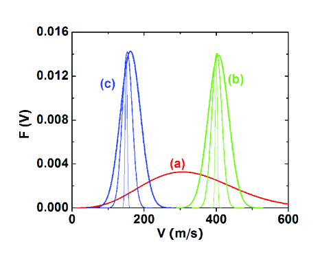
Figure 1: (Color online) Velocity distributions of molecular flux, $F(V)$, for beams formed (a) by effusive flow, (b) supersonic expansion from a stationary source, and (c) a rotating supersonic source, defined by Eqs.(4), (10), and (18), respectively. Parameters for (a) are $T_{0}=300K$; $\alpha=250$ m/s; for (b) and (c) flow velocities are $u=400$ m/s and $w=u+V_{rot}=250$ m/s and widths $\triangle v/u$ = 0.01, 0.05, 0.10. For (b) and (c) the widths also influence somewhat the most probable velocity.

These require only $\langle V^{k}\rangle$ , with k = 1 - 4, for the individual beams. We obtain analytic expressions for averages over velocity distributions for beams formed by effusive flow, by supersonic expansion, and by a rotating supersonic nozzle. Figure 1 illustrates these distributions. For the supersonic beams, three widths are shown; the broadest ($\sim$ 10%) is typical, the narrowest ($\sim$ 1%) is near the best achieved in Stark or Zeeman molecular decelerators exploiting phase stability and transverse focusing Meerakker ; Hogan . Results given here pertain to molecular flux distributions; as noted in an Appendix, they are readily adapted for number density distributions.

A. Effusive beams.

The flux distribution,

$$F(V)=V^{3}\text{exp}[-(V/\alpha)^{2}]$$ (4)

is governed by a single parameter, $\alpha=(2k_{B}T_{0}/m)^{1/2}$, with $k_{B}$ the Boltzmann constant, and $T_{0}$ the source temperature. The averaged powers of the velocity are

$$\langle(V/\alpha)^{k}\rangle=\int_{0}^{\infty}t^{k}F(t)dt/\int_{0}^{\infty}F(t)dt=\Gamma[(k+4)/2]$$ (5)

with $t=V/\alpha$ and $\Gamma(z)$ the Gamma function. The most probable velocity, $V_{mp}/\alpha=(3/2)^{1/2}=1.224$, and the rms velocity spread is $(\triangle V/\alpha)_{rms}=[2-(\tfrac{3}{4}\pi^{1/2})^{2}]^{1/2}=0.483$. The average beam kinetic energy is

$$\langle E_{BK}\rangle/(\tfrac{1}{2}m\alpha^{2})=\langle(V/\alpha)^{2}\rangle=2$$ (6)

and the rms kinetic energy spread is

$$\triangle E_{rms}/(\tfrac{1}{2}m\alpha^{2})=[\langle(V/\alpha)^{4}\rangle-\langle(V/\alpha)^{2}\rangle^{2}]^{1/2}=[\Gamma(4)-\Gamma^{2}(3)]^{1/2}=[6-4]^{1/2}=1.41$$ (7)

The spread thus is comparable to the beam kinetic energy.

For a merged pair of effusive beams, it is convenient to define $\alpha_{1}=\alpha_{12}\text{cos}\phi$, $\alpha_{2}=\alpha_{12}\text{sin}\phi$, with $\alpha_{12}=(\alpha_{1}^{2}+\alpha_{2}^{2})^{1/2}$, and $\langle v^{k}\rangle=\langle(V_{1}/\alpha_{1})^{k}\rangle=\langle(V_{2}/\alpha_{2})^{k}\rangle=\Gamma[(k+4)/2]$. The relative kinetic energy is

$$\langle E_{R}\rangle/(\tfrac{1}{2}\mu\alpha_{12}^{2})=\langle v^{2}\rangle-2\text{cs}\langle v\rangle^{2}\text{cos}\theta$$ (8)

with c = cos$\phi$ and s = sin$\phi$. The rms spread is

$$\triangle E_{R}/(\tfrac{1}{2}\mu\alpha_{12}^{2})=\left[A-B\text{cos}\theta+C\text{cos}^{2}\theta\right]^{1/2}$$ (9)

with

$$A=(c^{2}+s^{2})\left(\langle v^{4}\rangle-\langle v^{2}\rangle^{2}\right)$$

$$B=4cs\left(\langle v\rangle\langle v^{3}\rangle-\langle v\rangle^{2}\langle v^{2}\rangle\right)$$

$$C=4c^{2}s^{2}\left(\langle v^{2}\rangle^{2}-\langle v\rangle^{4}\right)$$

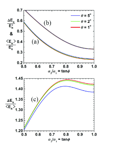
Figure 2: (Color online) Properties of merged effusive beams, from Eqs.(8) and (9), obtained by averaging over beam velocity distributions. (a) Averaged relative kinetic energy; (b) its rms spread; (c) ratio of spread to averaged kinetic energy, defining the available resolution. Ordinate energy scale is $E_{R}^{\circ}=\frac{1}{2}\mu(\alpha_{1}^{2}+\alpha_{2}^{2})$; abscissa scale pertains to ratio $\alpha_{2}/\alpha_{1}$ ranging from $\alpha_{2}=\frac{1}{2}\alpha_{1}$ to $\alpha_{2}=\alpha_{1}$. Results are shown for intersection angles of $\theta=1^{\circ}$, $2^{\circ}$ and $5^{\circ}$.

Figure 2 shows how $\langle E_{R}\rangle$ and $\triangle E_{R}$ vary with the ratio of beam velocities, which is proportional to $\alpha_{2}/\alpha_{1}=\text{tan}\phi$. The curves given are for intersection angles near zero, pertinent for merged beams. For matched beam velocities, with $\alpha_{2}=\alpha_{1}$, both $\langle E_{R}\rangle$ and $\triangle E_{R}$ are smallest. There, for small $\theta$, $\langle E_{R}\rangle$ and $\triangle E_{R}$ are less than the nominal relative kinetic energy, $E_{R}^{\circ}=\tfrac{1}{2}\mu(\alpha_{1}^{2}+\alpha_{2}^{2})$, for a perpendicular collision ($\theta=90^{\circ}$) by factors of only about 5 and 3, respectively. As $\alpha_{2}$ decreases below $\alpha_{1}$, $\langle E_{R}\rangle$ and $\triangle E_{R}$ increase in nearly parallel fashion. Accordingly, whether or not the merged beam velocities are closely matched, $\triangle E_{R}$ exceeds $\langle E_{R}\rangle$ appreciably (by $\sim$ 40% when $\alpha_{2}=\alpha_{1}$). The resolution of the relative kinetic energy hence is worse than seen in Eqs. (6) and (7) for the beam kinetic energy itself.

The velocity distribution for effusive beams is the same as for a bulk gas. Thus, $\langle E_{R}\rangle$ and $\triangle E_{R}$ for gas mixtures cooled by cryogenic means can be obtained from the merged beam results by merely setting $\text{cos}\theta=0$, equivalent to integrating over all angles of collision.

B. Stationary supersonic beams.

A standard approximation,

$$F(V)=V^{3}\text{exp}\{-[(V-u)/\triangle v]^{2}\}$$ (10)

for supersonic beams characterizes the velocity distribution by the flow velocity u along the centerline of the beam, and a width parameter $\triangle v=\alpha_{\|}=(2k_{B}T_{\|}/m)^{1/2}$, where $T_{\|}$, termed the parallel or longitudinal temperature, pertains to the molecular translational motion relative to the flow velocity Book1988 . According to the thermal conduction model Klots , $T_{\|}/T_{0}$ is determined by the pressure within the source, $P_{0}$, the nozzle diameter, $d$, and the heat capacity ratio, $\gamma=C_{P}/C_{V}$. Likewise, the flow velocity is given by

$$u=(2k_{B}T_{0}/m)^{1/2}[\gamma/(\gamma-1)]^{1/2}[1-(T_{\|}/T_{0})]^{1/2}$$ (11)

Analytic results for the velocity averages are readily obtained,

$$\langle(V/u)^{k}\rangle=P_{k+3}(x)/P_{3}(x)$$ (12)

with $x=\triangle v/u$ the ratio of velocity width to flow velocity, and

$$P_{n}(x)=\int_{0}^{\infty}t^{n}\text{exp}\{-[(t-1)/x]^{2}\}dt$$ (13)

with $t=V/u$. In the Appendix we give exact analytic formulas for the $P_{n}(x)$ functions; Table I provides polynomial approximations; for $x<0.3$ these are accurate to better than 0.03%.

The most probable velocity is $V_{mp}=\tfrac{1}{2}u\{1+[1+4x^{2}]^{1/2}\}\approx u(1+x^{2})$. The rms velocity spread is $(\triangle V/u)_{rms}=[P_{5}/P_{3}-(P_{4}/P_{3})^{2}]^{1/2}$. The corresponding average beam kinetic energy is

$$\langle E_{BK}\rangle/(\tfrac{1}{2}mu^{2})=P_{5}/P_{3}=\langle(V/u)^{2}\rangle$$ (14)

and the rms spread in kinetic energy is

$$\triangle E_{BK}/(\tfrac{1}{2}mu^{2})=\left[P_{7}/P_{3}-(P_{5}/P_{3})^{2}\right]^{1/2}$$ (15)

For a pair of merged supersonic beams, the averaged relative kinetic energy is

$$\langle E_{R}\rangle/(\tfrac{1}{2}\mu u_{12}^{2})=c^{2}\langle v_{1}^{2}\rangle+s^{2}\langle v_{2}^{2}\rangle-2\text{cs}\langle v_{1}\rangle\ \langle v_{2}\rangle\text{cos}\theta$$ (16)

where $u_{12}=(u_{1}^{2}+u_{2}^{2})^{1/2}$. The rms spread is

$$\triangle E_{R}/\left(\tfrac{1}{2}\mu u_{12}^{2}\right)=[A-B\text{cos}\theta+C\text{cos}^{2}\theta]^{1/2}$$ (17)

with

$$A=c^{4}\left[\langle v_{1}^{4}\rangle-\langle v_{1}^{2}\rangle^{2}\right]+s^{4}\left[\langle v_{2}^{4}\rangle-\langle v_{2}^{2}\rangle^{2}\right]$$

$$B=4cs\left[c^{2}\left(\langle v_{1}^{3}\rangle-\langle v_{1}\rangle\langle v_{1}^{2}\rangle\right)\langle v_{2}\rangle+s^{2}\left(\langle v_{2}^{3}\rangle-\langle v_{2}\rangle\langle v_{2}^{2}\rangle\right)\langle v_{1}\rangle\right]$$

$$C=4c^{2}s^{2}\left[\langle v_{1}^{2}\rangle\langle v_{2}^{2}\rangle-\langle v_{1}\rangle^{2}\langle v_{2}\rangle^{2}\right]$$

These expressions are akin to Eqs. (8) and (9), with $\alpha_{1}$ and $\alpha_{2}$ replaced by $u_{1}$ and $u_{2}$. Here $\langle v_{i}^{k}\rangle=\langle(V_{i}/u_{i})^{k}\rangle$, given by Eq.(12), may differ for the two beams ($i$ = 1, 2) if their velocity widths ($x_{i}=\triangle v_{i}/u_{i}$) differ.

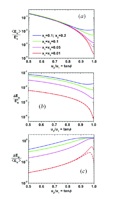
Figure 3: (Color online) Properties of merged supersonic beams, from Eqs.(16) and (17), obtained by averaging over beam velocity distributions. (a) Averaged relative kinetic energy; (b) its rms spread; (c) ratio of spread to averaged kinetic energy. For (a) and (b) the ordinate energy scale is $E_{R}^{\circ}=\frac{1}{2}\mu(u_{1}^{2}+u_{2}^{2})$. The abscissa scale pertains to the ratio $u_{2}/u_{1}$, which ranges from $u_{2}=\frac{1}{2}u_{1}$ to $u_{2}=u_{1}$. Results are shown for an intersection angle of $\theta=1^{\circ}$ and four sets of velocity spreads: $x_{1}=x_{2}$ = 0.01; 0.05; 0.1; and $x_{1}=0.1$, $x_{2}=0.2$. Dashed curves included for the $x=0.01$ case are for $\theta=2^{\circ}$.

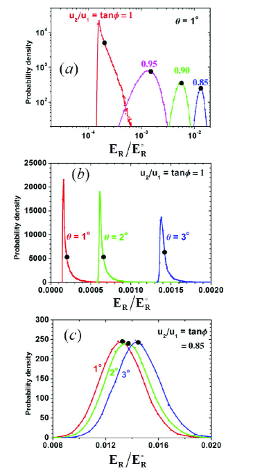
Figure 6: (Color online) Distributions of the relative kinetic energy, $P(E_{R})$, for merged supersonic beams from stationary sources. Values of $\langle E_{R}\rangle$ are indicated by black dots. Abscissa scale is in units of $E_{R}^{\circ}=\frac{1}{2}\mu\left(u_{1}^{2}+u_{2}^{2}\right)$, as used in Figs.3-5. (a) For merging angle $\theta=1^{\circ}$ and various ratios of the flow velocities, $u_{2}/u_{1}=1$ to 0.85 and velocity widths $x_{1}=x_{2}=0.01$. Note log-log plot is used. (b) For matched flow velocities, $u_{2}/u_{1}=1$ and $x=0.01$, but merging angle varied to illustrate its role in Eq.(20). (c) For flow velocities unmatched by $\sim$15% ($u_{1}u_{2}=0.85$) and $x=0.01$ with $\theta=1^{\circ}$, $2^{\circ}$, $3^{\circ}$, to illustrate the reduced role of the merging angle when the first term in Eq.(20) becomes predominant.

Figure 3 displays the dependence of $\langle E_{R}\rangle$ and $\triangle E_{R}$ on the ratio of flow velocities of the beams, $u_{2}/u_{1}=\text{tan}\phi$, and their velocity widths. Curves are shown for $\theta=1^{\circ}$ and $2^{\circ}$, to illustrate that the dependence on the merging angle is weak if the velocity widths of the beams are fairly large (cf. Fig.2) but for $\langle E_{R}\rangle$ becomes significant if the velocity widths are small (cf. Fig. 6 below). The dependence on the magnitude of the flow velocities is included simply by adopting units for $\langle E_{R}\rangle$ and $\triangle E_{R}$ that compare them with the relative kinetic energy for collisions at about the most probable beam velocities (nearly equal to $u_{1}$, $u_{2}$) at right angles ($\theta=90^{\circ}$), or equivalently in a bulk gas. We designate that by $E_{R}^{\circ}$. As seen in panel (a), if the merged beam velocities are precisely matched ($u_{2}=u_{1}$; $x_{2}=x_{1}$) the collision kinetic energy $\langle E_{R}\rangle$ is very sensitive to the velocity widths. In contrast, when the beam flow velocities are unmatched by more than about 15% (i.e., $u_{2}/u_{1}<0.85$), the ratio $\langle E_{R}\rangle/E_{R}^{\circ}$ becomes nearly independent of the velocity widths and grows larger as the unmatch increases. Panel (b) shows that regardless of whether the beam velocities are matched or not, the spread in relative kinetic energy, $\triangle E_{R}$, varies strongly with the velocity widths. Panel (c) plots the ratio $\triangle E_{R}/\langle E_{R}\rangle$, which defines the energy resolution. Whereas for closely matched beams $\langle E_{R}\rangle$ is minimal, $\triangle E_{R}$ then approaches its maximal value. Indeed, for matched beams with $x>0.05$, the resolution ratio, $\triangle E_{R}/\langle E_{R}\rangle$, is near $2^{1/2}$; that is just as poor as found in Fig. 2 for effusive beams.

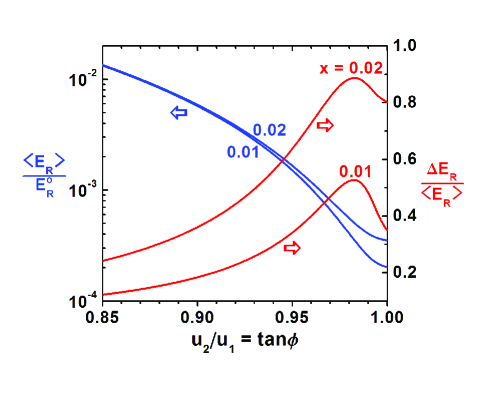
Figure 4: (Color online) Variation with extent of matching of merged beams flow velocities, $u_{2}/u_{1}$, for relative kinetic energy, $\langle E_{R}\rangle/E_{R}^{\circ}$ (left ordinate scale) and resolution ratio, $\triangle E_{R}/\langle E_{R}\rangle$ (right ordinate scale). Curves pertain to velocity spreads in beams of $x_{1}=x_{2}=0.01$ and 0.02 and merging angle of $\theta=1^{\circ}$.

To improve the resolution ratio for matched beams requires narrowing the velocity widths. Table II compares, both for the single beam and matched merged beams, effects of reducing the spread from $x$ = 0.1 to 0.01. For the single beam, the change in average kinetic energy is very slight, whereas the rms spread in the kinetic energy shrinks tenfold. For the merged beams, the relative kinetic energy is lowered by a factor of 25, and its rms spread by a factor of 100; so the resolution ratio is only improved fourfold. The resolution ratio can be lowered further if the merged beam velocities are unmatched, but that raises the averaged relative kinetic energy. Figure 4 displays the trade-offs involved. To obtain optimally low $\langle E_{R}\rangle$ requires nearly exact matching; that can provide $\langle E_{R}\rangle/E_{R}^{\circ}=2\times 10^{-4}$ for $x$ = 0.01 or $3\times 10^{-4}$ for $x$ = 0.02. However, for exact matching, the resolution ratio is only $\triangle E_{R}/\langle E_{R}\rangle$ = 0.35 for $x$ = 0.01 and surges to 0.8 for $x$ = 0.02. To attain resolution of 0.2 or 0.3 even with $x$ = 0.01 requires $u_{2}/u_{1}$ = 0.91 or 0.94 and hence would increase $\langle E_{R}\rangle/E_{R}^{\circ}$ to $\sim 5\times 10^{-3}$ or $2\times 10^{-3}$, respectively. The upshot is, to improve the resolution ratio by a factor of less than 2 (from 0.35 to 0.2) by unmatching, requires increasing $\langle E_{R}\rangle$ by a factor of 25.

Table 1: Approximate integrals for velocity averages.^a

$n$	$A_{n}(x,y)$
2	$4(2y^{2}+x^{2})x$
3	$4(2y^{2}+3x^{2})xy$
4	$2(4y^{4}+12x^{2}y^{2}+3x^{4})x$
5	$2(4y^{4}+20x^{2}y^{2}+15x^{4})xy$
6	$(8y^{6}+60x^{2}y^{4}+90x^{4}y^{2}+15x^{6})x$
7	$(8y^{6}+84x^{2}y^{4}+210x^{4}y^{2}+105x^{6})xy$

Table 2: Comparison of averages and spreads.^a

Quantity	Formula	$x=0.10$	$x=0.01$
$V_{mp}/u$	$\sim(1+x^{2})$	1.010	1.0001
$\triangle V/u$	$[(P_{5}/P_{3})-(P_{4}/P_{3})^{2}]^{1/2}$	0.070	0.0071
$\triangle V/V_{mp}$		0.070	0.0071
$\langle E_{BK}\rangle/(\tfrac{1}{2}mu^{2})$	$P_{5}/P_{3}$	1.035	1.0003
$\triangle E_{BK}/(\tfrac{1}{2}mu^{2})$	$[(P_{7}/P_{3})-(P_{5}/P_{3})^{2}]^{1/2}$	0.143	0.0141
$\triangle E_{BK}/\langle E_{BK}\rangle$		0.14	0.014
$\langle E_{R}\rangle/(\tfrac{1}{2}\mu u_{12}^{2})$	Eq.(16)	0.0051	0.00020
$\triangle E_{R}/(\tfrac{1}{2}\mu u_{12}^{2})$	Eq.(17)	0.00697	0.000071
$\triangle E_{R}/\langle E_{R}\rangle$		1.37	0.35

C. Rotating supersonic beams.

For a supersonic beam from a rotating source, the velocity distribution,

$$F(V)=V^{2}(V-V_{rot})\text{exp}\{-[(V-w)/\triangle v]^{2}\}$$ (18)

involves the peripheral velocity of the source, $V_{rot}$, which enters both in the $V-V_{rot}$ factor and in the flow velocity in the laboratory frame, $w=u+V_{rot}$, with $u$ again relative to the nozzle Gupta ; Strebel . In the slowing mode, when the rotor spins contrary to the beam exit flow, $V_{rot}<0$; in the speeding mode, $V\geq V_{rot}>0$. Also, in integrating over the velocity distribution of Eq. (18), the lower limit depends on the sign of $V_{rot}$. In the slowing mode, the lower limit is small (typically a few m$/$s) and represents a minimum, $V\geq V_{swat}$, necessary to allow molecules to escape swatting by the rotor. As noted in the Appendix, the swatting correction is extremely small, so we take $V_{swat}=0$. In the speeding mode, the lower limit may be large, since $V\geq V_{rot}$ is required. Here, in addition to $x=\triangle v/u$, it is convenient to specify two additional variables: $y=w/u$ and $z=V_{rot}/u$. The Appendix gives analytic results for the integrals, which are denoted by $P_{n}(x,y)$ for the slowing mode and $P_{n}(x,y,z)$ for the speeding mode. The corresponding velocity averages are given by

$$\langle(V/u)^{k}\rangle=(P_{k+3}-zP_{k+2})/(P_{3}-zP_{2})$$ (19)

where $P_{n}=P_{n}(x,y)$ or $P_{n}(x,y,z)$ for slowing or speeding ($z<0$ or $z>0$), respectively.

For merged beam experiments with neutral atoms or molecules, pairing a stationary supersonic source with a rotating source facilitates adjusting the relative flow velocity. For a stationary source, to adjust the flow velocity requires changing the temperature or, if the beam species of interest is seeded in a carrier gas, changing the seed ratio. That is awkward and imprecise. For the rotating source, the lab flow velocity, $w$, can be scanned easily and precisely by merely changing the rotor speed. The velocity width for a beam from the rotating source is likely to be wider, especially in the slowing mode (as $\triangle v/w>\triangle v/u$). However, it will often be desirable to further narrow the velocity spreads in both beams by means of electric or magnetic fields. Such narrowing operations can benefit from having the peak intensities of the beams preselcted to occur near the desired relative velocity.

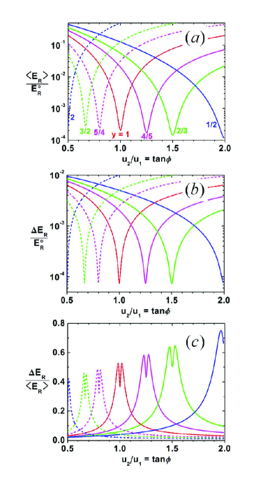
Figure 5: (Color online) Properties of merged supersonic beams, one from a stationary source, the other from a rotating source. As in Fig. 3, (a) shows the averaged relative kinetic energy; (b) its rms spread; (c) the resolution ratio, spread to averaged kinetic energy. Results shown are for $\theta=1^{\circ}$ and $x=0.01$. Both (a) and (b) exhibit pronounced minima where the matching condition holds: $w_{2}=u_{1}$ and hence $u_{2}/u_{1}=1/y$. Full curves show results for slowing mode, with $y=4/5$, $2/3$, and $1/2$; dashed curves are for speeding mode, with $y=5/4$, $3/2$, and 2.

The merged beam $\langle E_{R}\rangle$ and $\triangle E_{R}$ can be obtained from Eqs.(16) and (17), using $\langle v_{1}^{k}\rangle$ from Eq.(12) and $\langle v_{2}^{k}\rangle$ from Eq.(19). Figure 5 shows, for both slowing ($y<1$) and speeding modes ($y>1$), how results compare with those in Fig. 3 for a pair of stationary supersonic beams (y = 1). In panels (a) and (b), prominent minima occur where the flow velocities match: $w_{2}=yu_{2}=u_{1}$, hence $u_{2}/u_{1}=\text{tan}\phi=1/y$. In panel (c), the resolution ratio, $\triangle E_{R}/\langle E_{R}\rangle$, is least good (largest values) at the matching locations, but improves rapidly with modest unmatching, dropping to near 0.1 within $\sim$15% of the matching peaks.

D. Distribution of relative kinetic energy.

As seen in Figs. 3-5, to attain both low $\langle E_{R}\rangle$ and a small resolution ratio $\triangle E_{R}/\langle E_{R}\rangle$ requires that the merged beams have narrow velocity spreads. Even for $x\sim 0.01$, to get a resolution ratio below $\sim$0.35 requires that the most probable velocities differ somewhat. To examine further the competing aspects, we computed numerically the distribution $P(E_{R})$ of relative kinetic energy and its variation with the velocity spread, extent of unmatching, and the merging angle.

Figure 6 shows results for merged supersonic beams, both from stationary sources; results with one beam from a rotating source are similar. Panel (a) shows $P(E_{R})$ distributions for beams having velocity spreads of only 0.01 and merging angle $\theta=1^{\circ}$ with ratios of flow velocities $u_{2}/u_{1}$ = 1, 0.95, 0.90, and 0.85. Most striking is the form of $P(E_{R})$ when the beam velocities are both narrow and matched ($x=0.01$, $u_{2}=u_{1}$). Then the lower limit of the relative kinetic energy, $E_{R}/E_{R}^{\circ}<1.5\times 10^{-4}$, is sharply defined and $P(E_{R})$ resembles qualitatively a Poisson distribution. When the velocities become more and more unmatched $P(E_{R})$ becomes approximately Gaussian. In contrast, when the beam velocities are broader (e.g., $x=0.10$), the $P(E_{R})$ distribution is roughly Gaussian for both matched and modestly unmatched beam velocities.

Recasting Eq.(1) in the equivalent form,

$$E_{R}=\frac{1}{2}\mu\left[(V_{1}-V_{2})^{2}+4V_{1}V_{2}\text{sin}^{2}(\theta/2)\right]$$ (20)

makes evident why the lower limit for $E_{R}$ is sharply defined for merged beams with narrow, matched velocities. Then the first term in $E_{R}$ becomes very small, yet as long as $\theta\not=0$, the second term will be appreciable because the parent beam velocities are large. That second term will also be much less sensitive to velocity spreads; in Fig. 6, panels (b) and (c) exhibit its role.

III EXPERIMENTAL PROSPECTS

In study of chemical reactions at cold ($<$ 1 K) energies under single-collision conditions, constraints enter that differ from ”warm” (typically $>$ 300 K) molecular beam experiments. For reactions without electronic or vibrational excitation, cold reactive collisions cannot occur unless an activation barrier is absent or exceptionally low or thin. Such reactions are usually exoergic. The deBroglie wavelengths, long for the reactants, thus become very short for the products: ”waves in, particles out” Herschbach . Hence, disposal of energy and angular momentum among product states is virtually the same as in the warm regime. Also, as s-waves predominate in the entrance channel, the product angular distribution for cold collisions is typically isotropic or nearly so. Accordingly, dynamical features observable in warm collisions are not revealed in cold collisions. In the cold chemistry regime, the primary information to be sought is the integral reaction cross section and its dependence on relative kinetic energy or reactant excitation and/or interactions with external fields.

Merged beams are well suited for measurements of total reaction cross sections Phaneuf . The advantage at very low collision energies becomes immense as compared with experiments that slow both reactants, because the centerline flux in a molecular beam (whether effusive or supersonic) is proportional to the most probable velocity in the beam. Although merging imposes a very small angular spread, that is compensated because the reactant beams meet in a pencil-like volume, comparable in size to that in typical crossed-beam experiments. Merged beams are also congenial for use with pulsed sources, either stationary or rotating, which provide much higher intensity than continuous sources. Moreover, the option of overlapping reactants or not in time enhances S/N discrimination. Intensity is fostered too by the compactness of merged-beam geometry which also somewhat simplifies incorporating auxiliary apparatus.

In order to facilitate obtaining estimates for any choice of reactant atoms or molecules and velocity conditions, we have used unitless ratios in Figs. 2-6 and Table II. Here, in illustrative discussion of experimental options, we revert to customary units: energy in mK (or K); mass in amu, velocity in meters/sec. The merged beam technique can be used in many variants; we will consider just two that serve to exemplify basic aspects. We refer to these, somewhat whimsically, as ”ubiquitous” (ubiq) and ”utopian” (utop), to contrast what can be done using ordinary supersonic beams with that requiring much more ambitious, sophisticated apparatus.

Table III displays the chief distinction: for ubiq, $x\sim 0.1$ is typical, whereas for utop, $x\sim 0.01$ is as yet a challenging goal. The corresponding ranges of averaged collision energy and rms energy spread attainable are shown for either matched or 10% unmatched merged beams. As the overall energy scale is governed by $E_{R}^{\circ}=\tfrac{1}{2}\mu(u_{1}^{2}+u_{2}^{2})$, for either ubiq or utop to obtain the lowest $\langle E_{R}\rangle$ and $\triangle E_{R}$ requires that the reduced mass and most probable beam velocities be as small as feasible. Table III pertains to $\mu=1$ amu, available for reactions of an H atom with any considerably heavier reactant partner. The range of flow velocities considered, $u\sim 300$ to 600 m/s, extends as high as likely to be used. Even for light reactants, $u\sim 300$ m/s can be obtained by seeding in xenon carrier gas. That reduces intensity by a factor of typically $\sim 100$, but is routinely done as a precursor to most current methods for slowing molecules. Merged beams, especially if pulsed, can much better afford such a drop in intensity because further slowing is not required.

Table 3: Illustrative $\langle E_{R}\rangle$ and $\triangle E_{R}$ values.^a

$u_{1}$ (m/s)	$u_{2}$ (m/s)	$E_{R}^{\circ}$ (K)	$\langle E_{R}\rangle$ (mK)		$\triangle E_{R}$ (mK)
			$x=0.1$	$x=0.01$	$x=0.1$	$x=0.01$
600	600	43	215	9	290	3
500	500	30	150	6	200	2
400	400	19	95	4	130	1.3
300	300	11	55	2	75	0.7
600	540	39	390	195	460	39
500	450	27	270	135	320	27
400	360	17	170	85	200	17
300	270	10	100	50	120	10

As seen in Table III, the ubiq mode is capable of reaching $\langle E_{R}\rangle$ as low as $\sim$ 55 mK for H atom reactions. But, as evident in Figs 3 and 5, the rms energy spread is larger, so the resolution is miserable. In the cold collision regime, however, this is not as severe a limitation as might be expected. According to Wigner’s threshold law Wigner , for any exoergic inelastic or reactive collision at sufficiently low energy the cross section becomes proportional to $1/V_{R}$, so the rate coefficient becomes independent of the relative kinetic energy. State-of-the art quantum scattering calculations Quemener for a variety of inelastic and reactive processes indicate the Wigner regime is typically attained when $E_{R}$ drops below 100 mK ($<10^{-5}$ eV), which corresponds to a deBroglie wavelength of $\sim$ 40 nm or longer for H atoms.

To achieve the utop mode by shrinking the velocity spreads to only 1% of the most probable velocities, yet preserve adequate intensity, the best means presently in prospect appears to be deceleration by multistage Stark or Zeeman fields Hogan , likely exploiting transverse focusing and phase stability together with synchrotron-style storage rings Meeakker2 . Table III presumes the resultant velocity distributions resemble Eq.(10). If so, the utop mode should be able to lower $\langle E_{R}\rangle$ to $\sim$2 mK for H atom reactions, while reducing the energy spread to 0.7 mK, thereby improving the resolution to 35%, a rather modest level. As seen in Fig. 4 and Table II, in order to improve to the resolution to 20% would require that the beam velocities be unmatched by $\sim$10%, but that pushes $\langle E_{R}\rangle$ up to 50 mK. As the Wigner regime is readily accessible for H atom reactions, even for ubig, the elaborate experimental effort to attain utop would not be justified. Obtaining decent resolution would become much more worthwhile for reactions with considerably larger reduced mass, however. Then, even for utop, the Wigner regime would lie mostly beyond the accessible range.

IV DISCUSSION

In summary, the merged-beam technique has several inviting virtues. Foremost is the capability to study cold collisions with warm beams. In contrast to methods that require slowing both collision partners, the beam intensities can be much higher and the variety of molecular species used much wider. For collisions with small reduced mass, especially H or D atoms with heavy molecules, relative kinetic energy below 100 mK can be attained, using mostly standard, fairly simple molecular beam apparatus. However, to get low kinetic energy for collisions with large reduced mass, and/or to obtain decent energy resolution, will require making the beam velocity spreads very small ($\sim$1%), a challenging task which entails developing far more elaborate apparatus.

The merged-beam experiments implemented in our laboratory aim both to test the capabilities of ordinary, basic apparatus Sheffield and to explore in the cold regime H atom reactions that have been well studied in the warm domain. We note some indicative aspects. Pulsed supersonic sources are operated at high input pressures to enhance the familiar features of supersonic beams: high intensity, narrowed velocity spreads, drastic cooling of vibration and rotation. One source is stationary, the other rotating to enable readily adjusting its beam velocity to match that from its sedate partner. The rotor source is suitable for any fairly volatile molecule, while the stationary source can be used to generate species that must be produced from precursors, such as hydrogen, oxygen, or halogen atoms or free radicals. Initial experiments use the H + NO₂ $\longrightarrow$ OH + NO reaction. The H (or D) beam is supplied by dissociation of H₂ (or D₂) in an RF discharge source of exceptional efficiency, evolved from a design used in low-temperature NMR Boltnev . The H beam, seeded in Xe or Kr, has flow velocity in the range of 350 - 450 m/s and spread $\sim$10%. The rotating source provides the NO₂ beam, currently with estimated velocity spread $\sim$20%. With the beams merged at 420 m/s and $\theta=1.5^{\circ}$, the predicted $\langle E_{R}\rangle\sim 210$ mK and $\triangle E_{R}\sim 250$ mK. That is well within the ”cold” realm ($<$ 1 K), whereas the kinetic energy is $\sim$11 K for the H beam and $\sim$490 K for the NO₂ beam. The corresponding collisional deBroglie wavelength $\lambda_{R}\sim 27$ nm.

Here we have considered only effusive and supersonic beams, the most familiar. There is, however, a growing repertoire of other types, developed with focus on slowing. Some may offer properties advantageous for merged-beams, which shift the focus to narrowing velocity spreads. In particular, we mention the recently developed cryogenically cooled buffer gas beams Hutzler , which operate in the intermediate regime between effusive and supersonic flow. There the Knudsen number (essentially the ratio of Reynolds number and Mach number) is $Kn\sim 1-10^{-2}$, whereas for effusive beams $Kn>1$ and for supersonic beams typically $Kn\leq 10^{-3}$. In a prototype case producing a ThO beam Hutzler2 , a continuous gas flow maintains a stagnation density of Ne buffer gas in thermal equilibrium within a cell cooled to 18 K. A solid ThO₂ target is mounted to the cell wall. A YAG laser pulse vaporizes part of the target and ejects ThO molecules that are cooled by collision with the Ne buffer as they flow out of the cell. A key effect is ”hydrodynamic entrainment” that occurs when the time for the ThO molecules to exit the cell is less than the diffusion time to the cell walls. Remarkably, the molecular beam has intensity exceeding that for a supersonic beam, very low internal temperature, and its most probable velocity, governed by the cooling Ne, is $<$ 200 m/s. The velocity spread is broad, but the high intensity and low speed would permit much narrowing via velocity selection. Such cryogenically cooled and buffered beams seem likely to become widely applicable, perhaps along with merged-beams.

APPENDIX: INTEGRALS FOR VELOCITY AVERAGES

The averages, $\langle V^{k}\rangle$, over the velocity flux distributions specified in Eqs. (10) and (18) for supersonic beam sources involve two related integrals

$$P_{n}(x,y) = \int_{0}^{\infty}t^{n}\text{exp}\left[-\left(\frac{t-y}{x}\right)^{2}\right]dt$$ (A1)

$$= \frac{\sqrt{\pi}}{16}\left[1+\text{Erf}(y/x)\right]A_{n}(x,y)+\frac{x^{2}}{8}\text{exp}\left[-(y/x)^{2}\right]B_{n}(x,y)$$ (A2)

$$P_{n}(x,y,z) = \int_{z}^{\infty}t^{n}\text{exp}\left[-\left(\frac{t-y}{x}\right)^{2}\right]dt$$ (A3)

$$= \frac{\sqrt{\pi}}{16}\left[1+\text{Erf}(1/x)\right]A_{n}(x,y)+\frac{x^{2}}{8}\text{exp}\left[-(1/x)^{2}\right]\left[B_{n}(x,y)+C_{n}(x,y,z)\right]$$ (A4)

where, $n=k+3$, Erf is the error function, and $x=\triangle v/u$, $y=w/u$, $z=V_{rot}/u=y-1$. For a stationary source, only $P_{n}(x,1)$ enters, as $y=1$ and $z=0$; for a rotating source, $P_{n}(x,y)$ pertains to the slowing mode, with $0<y<1$ and $z<0$, and $P_{n}(x,y,z)$ to the speeding mode, with $y>1$ and $z>0$. Analytical formulas for the $A_{n}(x,y)$, $B_{n}(x,y)$ and $C_{n}(x,y,z)$ functions can be obtained by evaluating the $P_{n}$ in successive steps using integration by parts. Table I of the text gives, for $n$ = 2 to 7, explicit expressions for $A_{n}(x,y)$; Table IV below gives $B_{n}(x,y)$ and $C_{n}(x,y,z)$.

In the range of interest here, $x<0.3$ and $y>0.5$, the first term in Eqs. (A2) and (A4) is much larger than the others, and the error function is very close to unity. Accordingly, good approximations for $P_{n}(x,y)$ and $P_{n}(x,y,z)$ can be obtained by dropping the exponential part and replacing the Erf function by unity for compensation; thus,

$$P_{n}(x,y)\approx P_{n}(x,y,z)\approx\frac{\sqrt{\pi}}{8}A_{n}(x,y)=\sqrt{\pi}\sum_{s=0}^{[n/2]}\left(\begin{array}[]{c}n\\ 2s\end{array}\right)\frac{(2s-1)!!}{2^{s}}x^{2s+1}y^{n-2s}$$ (A7)

For $x<0.3$ and $y>0.5$, the error is $<0.03\%$. We note that the swatting correction mentioned under Eq.(18) of the text may be obtained from $\triangle P_{n}=P_{n}(x,y)-P_{n}(x,y,z*)$ with $z*=V_{swat}/u$. However, in the range of interest, $\triangle P_{n}$ is extremely small, much less than 0.03% so taking $V_{swat}=0$ is quite justified.

The velocity averages are given by

$$\langle(V/u)^{k}\rangle=(P_{k+3}-zP_{k+2})/(P_{3}-zP_{2})$$ (A8)

a generic formula that includes Eqs.(5), (12), and (19) of the text. For a stationary supersonic source, $P_{n}=P_{n}(x)=P_{n}(x,1)$; for a rotating source, $P_{n}=P_{n}(x,y)$ or $P_{n}(x,y,z)$ for slowing or speeding, respectively. The effusive beam case corresponds to $x=\alpha$, $y=0$, $z=0$, with $P_{n}(x,0)=\tfrac{1}{2}\alpha^{n+1}\Gamma[(n+1)/2]$. Results for averages over number density distributions rather than flux distributions can be obtained merely by setting $n=k+2$.

Table 4: Formulas for $B_{n}(x,y)$ and $C_{n}(x,y,z)$.

$n$	$B_{n}(x,y)$	$C_{n}(x,y,z)$
2	$4y$	$4z$
3	$4(y^{2}+x^{2})$	$4z(z+y)$
4	$2(2y^{2}+5x^{2})y$	$2[2z^{3}+2yz^{2}+(2y^{2}+3x^{2})z]$
5	$2(2y^{4}+9x^{2}y^{2}+4x^{4})$	$2[2z^{4}+2yz^{3}+2(y^{2}+x^{2})z^{2}+(2y^{3}+7x^{2}y)z]$
		$4z^{5}+4yz^{4}+2(5x^{2}+2y^{2})z^{3}+2(2y^{3}+9x^{2}y)z^{2}$
6	$(4y^{4}+28x^{2}y^{2}+33x^{4})y$	+$(4y^{4}+24x^{2}y^{2}+15x^{4})z$
		$4z^{6}+4yz^{5}+4(3x^{2}+y^{2})z^{4}+2(2y^{3}+11x^{2}y)z^{3}$
7	$4y^{6}+40x^{2}y^{4}+87x^{4}y^{2}+24x^{6}$	+$2(2y^{4}+15x^{2}y^{2}+12x^{4})z^{2}+(4y^{5}+36x^{2}y^{3}+57x^{4}y)z$

References

- (1) Cold Molecules: Theory, Experiment, Applications, R. V. Krems, W. C. Stwalley, and B. Friedrich, Eds., (Taylor and Francis, London, 2009).
- (2) Focus on Cold and Ultracold Molecules, L. D. Carr and J. Ye, Eds., New J. Phys. 11, 055009 (2009).
- (3) Cold and Ultracold Molecules, Faraday Disc. 142, (Royal Soc. Chem., London, 2009).
- (4) Physics and Chemistry of Cold Molecules, Phys. Chem. Chem. Phys. 13, 18703, O. Dulieu, R. Krems, M. Weidemuller, and S. Willitsch, Eds. (2011).
- (5) S. Ospelkaus, K.-K. Ni, D. Wang, M. H. G. de Miranda, B. Neyenhuis, G. Quemener, P. S. Julienne, J. L. Bohn, D.S. Jin, J. Ye, Science 327, 853 (2010).
- (6) M. H. G. de Miranda, A. Chotia, B. Neyenhis, D. Wang, G. Quemener, S. Ospelkaus, J. L. Bohn, J. Ye, D. S. Jin, Nature Physics 7, 502 (2011).
- (7) S. Y. T. van de Meerakker, H. L. Bethlem, and G. Meijer, Nature Physics 4, 595 (2008).
- (8) M. T. Bell and T. P. Softley, Mol. Phys. 107, 99 (2009).
- (9) S. D. Hogan, M. Motsch, and F. Merkt, Phys. Chem. Chem. Phys. 13, 18705 (2011).
- (10) L. Sheffield, M. Hickey, V. Krasovitsky, K. D. D. Rathnayaka, I. F. Lyuksyutov and D. R. Herschbach, Rev. Sci Instrum. (in press 2012).
- (11) R. A. Phaneuf, C. C. Havener, G. H. Dunn, and A. Muller, Rep. Prog. Phys. 62, 1143 (1999).
- (12) H. Pauly, in Atom, Molecule, and Cluster Beams, H. Pauly, Ed. (Springer, 2000), p. 8.
- (13) M. Gupta and D. Herschbach, J. Phys. Chem. A 105, 1626 (2001).
- (14) S. Y. T. van de Meeakker and G. Meijer, Faraday Disc. 142, 113 (2009).
- (15) D. R. Miller, in Atomic and Molecular Beam Methods, Vol. I, G. Scholes, Ed. (Oxford Univ. Press, New York, 1988), p. 14.
- (16) C. Klots, J. Chem. Phys. 72, 192 (1980).
- (17) M. Strebel, F. Stienkemeier, and M. Mudrich, Phys. Rev. A 81, 033409 (2010).
- (18) D. Herschbach, Faraday Disc. 142, 9 (2009).
- (19) E. P. Wigner, Phys. Rev. 73, 1002 (1948).
- (20) G. Quemener, N. Balakrishnan and A. Dalgarno, Inelastic collisions and chemical reactions of molecules at ultracold temperatures, in Cold Molecules: Theory, Experiment, Applications, R. V. Krems, W. C. Stwalley, and B. Friedrich, Eds., (Taylor and Francis, London, 2009), p. 69.
- (21) R. E. Boltnev, V. V. Khmelenko, and D. M. Lee, Low Temp. Phys. 36, 382 (2010).
- (22) N. R. Hutzler, H.-I Lu, and J. M. Doyle, Chemical Reviews (in press).
- (23) N. R. Hutzler, M. F. Parsons, Y. V. Gurevich, P. W. Hess, E. Petrik, B. Spaun, A. C. Vutha, D. DeMille, G. Gabrielse, J. M. Doyle, Phys. Chem. Chem. Phys. 13, 18976 (2011).