Probing deviations from General Relativity with the Euclid spectroscopic survey
Abstract
We discuss the ability of the planned Euclid mission to detect deviations from General Relativity using its extensive redshift survey of more than 50 Million galaxies. Constraints on the gravity theory are placed measuring the growth rate of structure within 14 redshift bins between and . The growth rate is measured from redshift-space distortions, i.e. the anisotropy of the clustering pattern induced by coherent peculiar motions. This is performed in the overall context of the Euclid spectroscopic survey, which will simultaneously measure the expansion history of the universe, using the power spectrum and its baryonic features as a standard ruler, accounting for the relative degeneracies of expansion and growth parameters. The resulting expected errors on the growth rate in the different redshift bins, expressed through the quantity , range between and . We discuss the optimisation of the survey configuration and investigate the important dependence on the growth parameterisation and the assumed cosmological model. We show how a specific parameterisation could actually drive the design towards artificially restricted regions of the parameter space. Finally, in the framework of the popular “ parameterisation”, we show that the Euclid spectroscopic survey alone will already be able to provide substantial evidence (in Bayesian terms) if the growth index differs from the GR value by at least . This will combine with the comparable inference power provided by the Euclid weak lensing survey, resulting in Euclid’s unique ability to provide a decisive test of modified gravity.
keywords:
cosmology – dark energy – large-scale structure of universe.1 Introduction
The current standard cosmological model, concordantly supported by virtually all available observations, tells us that we live in a low-density, expanding universe with a spatially flat geometry, that appears to have recently entered a phase of accelerated expansion. The data require an extra mass-energy contribution in the form of a fluid with equation of state . This corresponds to adding in the equations of General Relativity (GR) a cosmological constant , i.e. the term originally introduced by Einstein to obtain a static solution, thus building the standard Lambda Cold Dark Matter model (LCDM). A cosmological constant, however, has a few disturbing features. The first feature is the fine tuning necessary to obtain its measured density value, which can be interpreted as the energy of the vacuum, that is extremely small compared to the corresponding scales of particle physics; the second issue is the so-called coincidence problem: why, despite very different time evolutions, do dust-like matter and cosmological constant show comparable densities today? Among possible solutions, scenarios with evolving ‘dark energy’ density from a cosmological scalar field, have been proposed (see Frieman et al. 2008 for a review). Alternatively, however, observations could simply indicate that it is the theory of gravity that needs to be revised (see Copeland et al. 2006 for a review).
These two radically different explanations cannot be distinguished by measuring only the expansion history of the universe represented by the Hubble function . A way to break this degeneracy is to look at the linear growth rate of density perturbations. This can be expressed as lnln, where is the time-dependent part of the solution of the linear growth equation (Heath, 1977) and is the cosmic scale factor. Models with the same expansion history , but based on a different gravity theory predict a different growth rate (Maartens, 2007; Linder, 2005; Polarski, 2006) (although see also Kunz & Sapone 2007 for possible issues).
Measurements of galaxy clustering from large redshift surveys, quantified through the galaxy-galaxy correlation function (or its Fourier transform, the power spectrum ), contain direct information on both and .
Baryonic Acoustic Oscillations (BAO) within the last-scattering surface give rise to a characteristic feature in the galaxy distribution at comoving separations of Mpc (BAO have now been conclusively seen in the clustering of galaxies, e.g. Cole et al. 2005; Eisenstein et al. 2005 and more recently Kazin et al. 2010). This corresponds to the characteristic scale fixed by the comoving sound horizon at the drag epoch (shortly after recombination) and is accurately measured by Cosmic Microwave Background (CMB) anisotropies (see recent measurements by Komatsu et al. 2009). Compared to the observed galaxy BAO peak position at different redshifts, this yields a measurement of in the radial direction and of the comoving angular diameter distance in the transverse direction.
Galaxy clustering as measured in redshift space also contains the imprint of the linear growth rate of structure, in the form of a measurable anisotropy. Such redshift-space distortion (RSD) is due to coherent flows of matter from low to high densities, linked to the growth of structure. When redshifts are used to measure galaxy distances, the contribution from peculiar velocities produces a distortion of the clustering pattern, which at linear scales is proportional to (Kaiser, 1987; Hamilton, 1998). This can be measured by modelling the anisotropy of redshift-space two-point statistics, defining a proper correlation function (or power spectrum ), where and ( and ) are the components parallel (perpendicular) to the line of sight. The anisotropy is caused by an additive term proportional to the variance of the velocity field, which can be parameterised by (where is the rms amplitude of galaxy clustering) and provides an excellent discriminator of cosmological models, particularly if is normalised, for example using the CMB (Song & Percival, 2009).
RSD were classically seen as a method to measure (see references in Hamilton (1998) or more recently Hawkins et al. (2003), Ross et al. (2007), da Angela et al. (2008), Cabre & Gaztanaga (2009), Drinkwater et al. (2010)). In the dark energy context, they were initially seen as simply an effect to be corrected for to extract the full BAO information (Seo & Eisenstein, 2003). Still in the context of GR, Amendola et al. (2005) showed that the information contained in the GR growth function could improve errors on parameters by (see also Sapone & Amendola 2007). As pointed out by Guzzo et al. (2008), however, if no assumption is made on the gravity theory, RSD in fact provide us with a powerful test to test the dark energy vs modified gravity alternative by tracing the growth rate back in time. This was particularly interesting in the context of planned dark energy surveys, and stimulated new interest in this technique (Wang, 2008; Linder, 2008; Nesseris & Perivolaropoulos, 2008; Acquaviva et al., 2008; Song & Percival, 2009; White et al., 2008a; Percival & White, 2009). Following Guzzo et al. (2008), RSD were suggested as a primary probe in the SPACE satellite proposal (the forerunner of what is now the Euclid spectroscopic probe, described in more detail below) presented in response to the 2007 ESA Cosmic Vision Call (Cimatti et al., 2009).
Currently ongoing spectroscopic surveys such as WiggleZ (Blake et al., 2011), BOSS (White et al., 2011) and VIPERS (Guzzo et al. 2012, in preparation), are mapping significant volumes of the distant universe and will produce measurements of covering the redshift range out to . Even larger and deeper galaxy surveys are planned for the next ten years, both from ground and space. These are the proposed BigBOSS (Schlegel et al., 2011) project using the refurbished KPNO and CTIO 4m telescopes, and, most importantly, the ultimate redshift survey from space by the approved ESA mission Euclid (Laureijs, 2009) we already mentioned above. Main aim of these projects is precisely the solution of the dark energy puzzle. In particular, Euclid is a medium-size (M-class) mission of the ESA Cosmic Vision programme, which has recently been selected for implementation, with launch planned for 2019. Euclid will perform both a photometric survey in the visible and in three near-infrared bands, to measure weak gravitational lensing by imaging billion galaxies, plus a spectroscopic slitless survey of galaxies. Both surveys will be able to constrain both the expansion and growth histories of the universe. Their combination makes Euclid a unique experiment, with superb precision and optimal cross-control of systematic effects (see Laureijs et al. 2011). In this paper we present the expected performances of the spectroscopic survey, as described in the Euclid Definition Study Report111http://www.euclid-ec.org (Laureijs et al., 2011), in quantifying the growth history and test for possible modifications of gravity as the origin of cosmic acceleration.
We shall first explore the forecasted constraints on the growth rate both for the expected survey parameters, and for a pessimistic galaxy density reduced by a factor of two. We will use the well-known parameterisation of the growth rate (Peebles, 1980; Fry, 1985; Lightman & Schechter, 1990; Wang & Steinhardt, 1998), where , is the matter energy density and is the critical density making the universe spatially flat, to look at future constraints on the parameter , which characterises the gravity model, and test degeneracies arising when making assumptions on the background cosmology.
We will then look at how constraints on growth are modified when survey specifications are changed, such as the total covered area and the corresponding galaxy number density (see discussion in Sec. 6) and the redshift range covered by the survey. In order to do this we need a measure of the quality of our growth constraint. For this reason we introduce a new simple Figure of Merit (FoM), analogous to the dark energy FoM defined in the Dark Energy Task Force Report (Albrecht et al., 2006). We then show how this FoM depends on the already mentioned survey specifications.
Expressing as a function of when considering sub-horizon matter perturbation is a well justified choice for GR cosmologies and for some modified gravity theories (e.g. the DGP model, a well-known five-dimensional model proposed in Dvali et al. 2000 where the acceleration of the expansion is due to the leakage of gravity into an extra dimension) but it is not the only possibility. In some cases a constant cannot describe the growth rate, as shown, for example, by Di Porto & Amendola (2008) for a class of models of dark energy coupled to matter. Therefore, when optimising a survey configuration for the growth rate measurement, it is important to consider not only one parameterisation of , in order not to bias our decisions. The same was shown for the case of the equation of state parameterisation in Wang et al. (2010). To have a more general perspective, we take a second growth parameterisation and compare the results obtained. We choose the parameterisation proposed by Pogosian et al. (2010), Song et al. (2011) which is physical, works at any scale and it is also able to reproduce the DGP growth rate.
Finally, we focus on the specific question “will the Euclid spectroscopic survey be able to distinguish between GR and modified gravity models?” To answer it, we use a Bayesian approach, following the work of Heavens et al. (2007). Here, a way to forecast the Bayesian evidence is proposed, based on Fisher statistics. In particular, we look at how much of a modified gravity model has to differ from the GR value in order for our fiducial survey to be able to distinguish it.
Our work extends that of Wang et al. (2010), who considered using a Euclid-like survey to measure the dark energy equation of state, to further consider the growth rate of structure. It confirms the results of Simpson & Peacock (2010) and Samushia et al. (2011), who specifically focused on cosmological model dependence. Parallel work that appeared while this paper was in preparation includes that of Di Porto et al. (2011), who look at bias and time-dependent parameterisations of , while we specialise on different growth parameterisations and on the dependence on survey specifications,Belloso et al. (2011), who find an exact solution of and Ziaeepour (2011), who estimate constraints from wide surveys based on a new growth parameterisation for modified gravity and interacting dark energy models. A difference between our work and all the papers mentioned above is that our results are updated to the latest Euclid configuration (Laureijs et al., 2011), which includes results from the most accurate simulations of the instrument.
The outline of the paper is the following. In Sec. 2 we describe RSD as an observable to measure growth, while in Sec. 3 the Fisher matrix method used to forecast errors on growth and other cosmological parameters is outlined, and the fiducial cosmology is defined. Sec. 4 describes how the survey was modelled, while Sec. 5 shows our forecasts, and in the following Sec. 6 we define the growth Figure of Merit, which we apply to our forecasted survey data. In Sec. 7 we compute the forecasted Bayesian evidence and we finally conclude in Sec. 8. Appendix A contains a brief review of the theory of the growth of linear small-scale perturbations and of growth parameterisations used in the literature.
2 Measuring growth: redshift space distortions
Our observable, containing both BAO and RSD, is the galaxy power spectrum. We write the observed power spectrum as (Kaiser, 1987; Seo & Eisenstein, 2003; Song & Percival, 2009)
| (1) | |||||
where the subscript r indicates quantities in the reference cosmology chosen to compute the power spectrum, , are the wave modes perpendicular and parallel to the line-of-sight, , and is a scale-independent offset due to imperfect removal of shot-noise. The term represents the distortion of the power spectrum due to the Alcock-Paczynski effect (Alcock & Paczynski, 1979), which also has the impact of changing the true into reference .
Notice here that the term is independent of the normalisation of the matter power spectrum.
We allow for the growth of structure to vary away from that of a LCDM model in two directions. First we allow the growth rate, which is well approximated by ( for curved space, Gong et al., 2009) with in LCDM models, to have . Second, we directly allow a modification of the standard equation for the time-like metric potential . This modification is described following Pogosian et al. (2010); Song et al. (2011) by a constant parameter . This choice and its motivation are discussed in more detail in Appendix A. We will use these parameters to model growth from observations of redshift-space distortions.
3 Forecasting the errors
In this section we give details of the method used to estimate the expected minimum errors obtainable on or and the other cosmological parameters from future redshift surveys, once the measurement error on the observables is known.
To perform our forecasts we use the standard Fisher matrix approach which was introduced to forecast errors on and derived parameters (Tegmark, 1997) and then adapted by Seo & Eisenstein (2003) to the measurement of distances using the BAO position, avoiding the “noise” of RSD. A series of papers in the literature have then used and discussed this technique to extract the information on both expansion and growth (for example recently Wang 2008; White et al. 2008b; Simpson & Peacock 2010; Wang et al. 2010; Samushia et al. 2011; Di Porto et al. 2011). Here we follow in particular the approximations discussed in Samushia et al. (2011).
Briefly, the Fisher matrix is defined as (see e.g. Bassett et al. 2009) , where is the likelihood function and are the model parameters whose error one wishes to forecast. It is possible to show that the Fisher matrix is the inverse of the covariance matrix, , in the (strong) assumption that the likelihood is a Gaussian function of the parameters and not only of the data. The galaxy power spectrum Fisher matrix can be approximated as (Tegmark, 1997)
| (2) |
where is the galaxy power spectrum, Eq. (1), and its derivatives are computed in a chosen fiducial model, , is the volume of the survey and is the galaxy number density.
Following Samushia et al. (2011), we neglect , since this term should only introduce negligible error. We also neglect the dependence of on , , and . This means that we do not use the information coming from the shape of the matter power spectrum. We finally multiply the integrand of the Fisher Matrix by a factor accounting for a possible error in redshift, , where is the standard deviation of the redshift error expected in Euclid. In each redshift bin centred at we compute a Fisher matrix (Seo & Eisenstein, 2003) with parameters
| (3) |
where in different redshift bins are considered to be independent; then all the matrices corresponding to all are summed. From the total Fisher matrix it is possible to estimate the errors on each in each redshift bin, by marginalising over all other parameters. To obtain errors on cosmological parameters, we marginalise over and project the obtained matrix into the final cosmological parameter set.
Regarding the latter, we test three nested models: 1) a simple quasi-LCDM with a constant fixed to instead of as in LCDM, which we dub qLCDM222We take to match the choice of Laureijs et al. (2011), motivated by the possibility of computing cosmological perturbations avoiding the barrier., 2) a model where dark energy has constant equation of state , dubbed wCDM and 3) a model where the equation of state of dark energy is allowed to vary, following the evolution , which we call CPL (Chevallier & Polarski, 2001; Linder, 2003). For all these models we consider both the flat and the curved space cases. The full set of parameters, from which we pick the appropriate subset according to the chosen model, is therefore
| (4) |
where . This is different from Samushia et al. (2011) since they do not consider and their resulting errors will be consequently smaller with respect to this work, as we will see in Sec. 5.
Our fiducial model is, as in the Euclid Definition Report, a flat constant cosmology with parameter values as the best-fit WMAP-7 (Komatsu et al., 2011) results (except for ):
| (5) |
The fiducial matter power spectrum for this cosmology is computed using CAMB333http://camb.info (Lewis et al., 2000).
We assume a scale-independent bias, which is a good approximation for large enough scales. As a fiducial bias, we take the bias function derived by Orsi et al. (2009) using a semi-analytical model of galaxy formation. For an analysis of how the bias can be constrained and of the impact of assuming a biasing model on the estimates of the growth factor we refer to the parallel work of Di Porto et al. (2011). Number densities and biasing parameters are summarised in Table 1, together with the integration limits in . The latter correspond to scales such that , with an additional cut at .
In a separate paper, Bianchi et al. (2012) perform a detailed study of statistical and systematic errors in RSD measurements, using a large set of mock surveys built from numerical simulations. They compare their results with predictions from the Fisher matrix code used here, finding fairly good agreement when considering only linear scales.
4 Modelling the Euclid Survey
Euclid will cover an area of in both imaging and spectroscopy (Laureijs et al., 2011), measuring redshifts in the infrared band () for Million galaxies, using a slitless spectrograph. With this technique, the redshift measurement relies on the detection of emission lines in the galaxy spectra, which in the chosen wavelength range in the vast majority of cases will be the line, redshifted to .
Intrinsic to the slitless technique is the impossibility to define a priori a survey flux limit (as normally done in a classical slit survey, which is based on a well defined target sample selected to a given magnitude or flux limit). Spectra are intrinsically confused by superpositions and the actual flux limit depends not only on the nominal signal-to-noise reachable through a given exposure, but also and fundamentally on the strategy devised as to resolve the confusion among the different spectra. In the case of Euclid, this is achieved first by splitting the wavelength range into two sub-exposures through a “blue” and a “red” grisms, covering respectively the wavelength ranges and ; this has the advantage of halving the length of the spectra on the detector, thus reducing superpositions. Secondly, the blue and red exposures are in turn split into two sub-exposures, observed rotating the field of view by . This makes for four different exposures of a given field, which result in a sensible treatment of spectral confusion. To verify this and compute the success rate of the survey (i.e. the fraction of correctly measured redshifts over the total number of spectra), it was necessary to develop since the early stages of the project an advanced end-to-end simulation pipeline. An accurate description of these simulations is beyond the scope of this paper, and we refer the reader to the Euclid Definition Study Report (Laureijs et al., 2011), and to the specific paper (Garilli et al. 2012, in preparation). Here we recall only the main concepts, which are relevant for the present analysis.
The end-to-end spectroscopic simulations take into account Euclid’s instrumental (point-spread function, resolution and instrumental background) and observational (exposure time, astrophysical background) parameters, to build an artificial “observation” of a realistic galaxy field. The input data set is built starting from the COSMOS catalogue of photometric redshifts (Ilbert et al., 2009), which contains all relevant information (coordinates, redshift, luminosity, spectral energy distribution, stellar formation rate, etc.). Most importantly, the COSMOS depth and extensive wavelength coverage (over 30 spectral bands), allows us to assign a well-defined spectral type and thus a realistic distribution of equivalent widths, down to large distances. It is also important that, being based on real observations, the catalogue includes also a realistic clustering of the sources. Stars are then added upon the galaxy catalogue. The package aXeSIM3 is then used to generate the four 2D dispersed images of the field and then extract the four 1D spectra for each target. Redshift are measured making use of RESS (Redshift Evaluation from Slitless Spectroscopy), an automatic software running within IRAF environment, which has been devised (Rossetti E. 2012, in preparation) to reduce and analyse highly contaminated slitless spectra. RESS’ measure is currently implemented only for low galaxies () and its extension for high objects is in progress. Redshift evaluation is based on the position of the line and any other emission lines, when detected, for which a flux is also measured. A reliability flag for each measured redshift is then obtained by further processing the spectra through the EZ redshift measurement code (Garilli et al., 2010). Comparison of the input and output catalogues allows one to estimate the success rate of the survey in terms of completeness and purity as a function of redshift and flux (see Euclid Definition Study Report, Fig. 6.10). Rather than trusting the absolute redshift distribution emerging from the simulated field, a more conservative choice is to use this output as weight, to be applied to the most up-to-date predictions for the redshift distribution of emitters (Geach et al., 2008). This produces the expected distribution of the number of galaxies with measured redshift in each redshift bin. From this one can calculate the galaxy number density at each , which is shown in Fig. 1 for our fiducial cosmology of Eq. (5).

5 Standard predictions for Euclid
For our computations here, we split the Euclid predicted redshift distribution over the range , into 14 bins with . Using the predicted galaxy number density in each bin shown in Fig. 1, we obtain the error on our observable, the power spectrum, and estimate the resulting precision on the measurement of after marginalisation over the other parameters. We plot errors on in Fig. 2 (dark blue error bars), where we also show for comparison current measurements of (light pink and magenta error bars) and the pessimistic case of observing only half the number of galaxies forecasted in Geach et al. (2008) (light blue error bars), as the authors themselves claim that their counts may be wrong by a factor of 2.
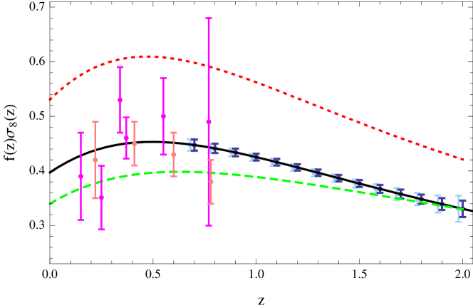
Current measurements shown in Fig. 2 are listed in Table 2. The values of are computed in the case of Guzzo et al. (2008) and Hawkins et al. (2003) by using the value of given by the authors and computing from and the reference cosmology they adopt for the computation of (or of Lahav et al. 2002 in the case of Hawkins et al. 2003); in the case of Ross et al. (2007) was computed using the expression444This formula actually gives us the non-linear , since we have used the non linear estimate of of Ross et al. (2007) to compute it. What we needed to obtain the linear would be the linear , but we do not have it. Therefore our estimate of for the Ross et al. (2007) datapoint might be higher than it should. (Zehavi et al., 2005), . Cabre & Gaztanaga (2009) indicate directly their value of , while Blake et al. (2011) and Samushia et al. (2011) compute directly . Error bars are obtained through the error propagation formula for uncorrelated data, when not directly specified in the papers.
| survey | reference paper | ||
|---|---|---|---|
| VVDS F22 | Guzzo et al. (2008) | ||
| wide | |||
| 2SLAQ | Ross et al. (2007) | ||
| galaxy | |||
| SDSS LRG | Cabre & Gaztanaga (2009) | ||
| Samushia et al. (2011) | |||
| 2dFGRS | Hawkins et al. (2003) | ||
| WiggleZ | Blake et al. (2011) | ||
Together with the (solid black) curve representing our fiducial , we also show for comparison a (dashed green) line for flat DGP, (calculated by numerical integration of the corresponding equation for ) and a (dotted red) line for the coupled model of Di Porto et al. (2011), computed using the parameterisation of Di Porto & Amendola (2008) with a coupling (both with and the same of our fiducial model).
We notice that we reach accuracies between and in the measurement of depending on the redshift bin, where the highest precision is reached for redshifts .
5.1 Comparison to other surveys
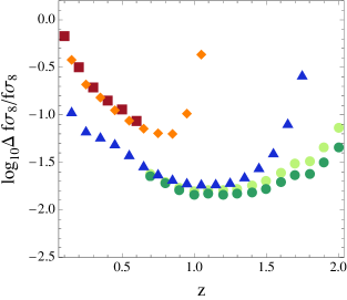
Together with Euclid, other ongoing and future surveys will constrain cosmology by measuring . Here we compare the relative errors on obtained using different spectroscopic galaxy redshift surveys. In particular, we consider the BOSS survey555http://cosmology.lbl.gov/BOSS/ (see Schlegel et al. 2009) and the BigBOSS666http://bigboss.lbl.gov/ Emission Line Galaxies (ELGs) and Luminous Red Galaxies (LRGs)777We thank the BigBOSS consortium for providing their latest yet unpublished estimate of their expected galaxy densities, which we used in creating this plot.. Regarding the fiducial bias, we use the forecasts by Orsi et al. (2009) for BigBOSS ELGs. We use (where is the standard linear growth rate) for BOSS and BigBOSS LRGs (see Reid et al. (2010)). Table 3 summarises the main characteristics of these surveys.
| survey | redshift range | area | bias | |
|---|---|---|---|---|
| BOSS LRG | ||||
| BigBOSS LRG | unpublished (see footnote 7) | |||
| BigBOSS ELG | unpublished (see footnote 7) | see Orsi et al. (2009) |
The results are shown in Fig. 3. We first notice that Euclid (represented by dark-green circles) will obtain the most precise measurements of growth, even in the pessimistic situation of detecting only half the galaxies (light-green circles). In redshift coverage it will be perfectly complementary to BOSS. The partial overlap with BigBOSS, whose ELG sample will reach similar errors up to , will allow for interesting and useful independent measurements and cross-checks.
5.2 Cosmological parameters
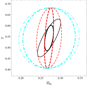
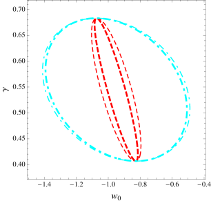
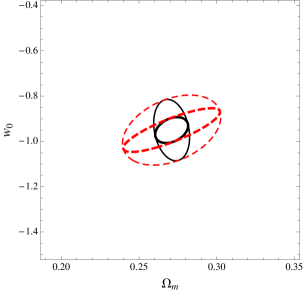
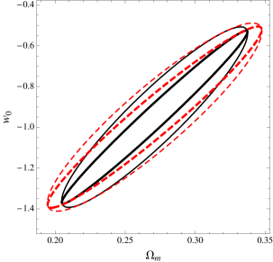
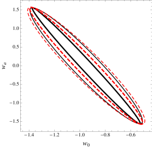
We next look at how the errors on , and project into errors on cosmological parameters. We only show results for and briefly mention results for (see Appendix B for more detailed error forecasts), while in the next section we will compare the two parameterisations and . In order to understand the model-dependence of these forecasts, we use the nested cosmologies described in Sec. 2: the more complicated model is a generalisation of the less complicated one, and the generalisation consists in the addition of one extra parameter. We also study the influence in the estimate of background parameters of assuming GR or allowing for a different constant . Results are shown in Figs. 4-7.
From Fig. 4 and 5, and by comparing left with right panel of Fig. 6 it is clear that what affects most strongly the error estimate, by enlarging the ellipses and even changing the degeneracy direction of parameters, is the assumption of different dark energy models. The assumption of zero curvature also has an influence. The less parameters the cosmological model possesses, the stronger is the influence of fixing , as can be seen from Fig. 4 (compare thick and thin lines having the same line style/colour) and Fig. 6 (compare solid and dashed lines with same thickness). affects more strongly the measure of background parameters, and only indirectly constraints on (note the thickening of error ellipses in Fig. 4 in the direction of background parameters and , respectively).
As regards the parameterisation, the error on is forecasted to be between and , depending on the dark energy model. The assumptions on and those on affect more strongly constraints on this growth parameter, in the case of the error ellipses.
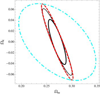
The assumption of GR has a different influence on different pairs of parameters. As regards , we can see from Fig. 5 that fixing reduces only the error for qLCDM, while errors on wCDM and CPL are unaffected. Errors on are very weakly affected by the assumption of GR and also of zero curvature (see Fig. 7), so that their determination is rather robust. This conclusion agrees with what obtained in Samushia et al. (2011) (see their Figs. 4 (a) and 5 (a) of the final published version), where the small differences are due to the presence of an extra parameter in our analysis over which we marginalise, namely and to the different survey specifications. The different degeneration direction of is due to the wrong sign convention being adopted in figure 5 of Samushia et al. (2011) which had the effect of inverting the axis. We have checked that our code gives exactly the same results as Samushia et al. (2011) if the parameter is fixed and the survey specifications are identical. The pair of parameters which is most affected by the choice of fixing is , more strongly in the case of wCDM, as can be seen in Fig. 6.
5.3 Adding Planck
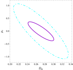
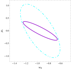
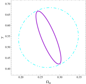
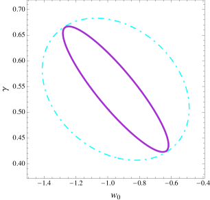
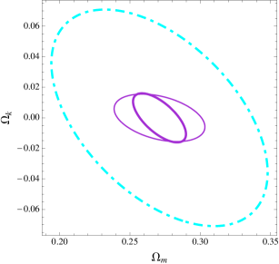
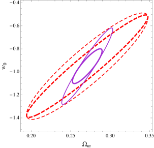
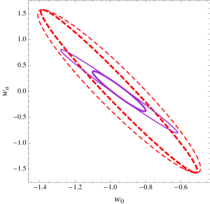
We then quantify the impact of adding Planck constraints to the Euclid spectroscopic survey constraints, to check how much errors reduce. The Planck satellite (part of the Cosmic Vision programme by the European Space Agency) has been launched in 2009 and it is presently operating (Tauber et al., 2010). Its results on cosmology will be made public in the next years and will be the state-of-the-art data on CMB temperature and polarisation. It is natural and convenient to combine these data to Euclid galaxy survey data, first of all because these probes are highly complementary, observing the early and late universe respectively, and secondly because of the presence of the BAO feature in both datasets. As in Samushia et al. (2011), we utilise the Dark Energy Task Force Planck Fisher, computed for 8 parameters: , , , , , , and . Since this Fisher matrix is computed assuming GR, to generalise it for arbitrary in order to sum it to our galaxy survey Fisher matrix, we use the same method as in Samushia et al. (2011) (see their Appendix B for details). In Figs. 8-11 we compare errors with (solid purple lines) and without (red-dashed or cyan dot-dashed lines) adding Planck, for a CPL dark energy.
As can be seen from Fig. 8, Planck noticeably improves marginalised errors on , obviously by constraining the background parameters. The error most reduced by Planck is, as one expects, that on (see Fig. 9), quite independently of the assumptions on growth (compare thick lines-corresponding to assuming GR, to thin lines–where is not fixed). As regards constraints on the alternative parameterisation, here the impact of adding Planck data on combined and constraints is stronger than for : the projected error on is reduced from to . This is shown in more detail in Appendix B. Joint Euclid-Planck constraints on (Fig. 10) and (Fig. 11) depend more strongly on the assumption on , but are in any case a decisive improvement with respect to Euclid-only constraints. This is again consistent with what obtained by Samushia et al. (2011), who find slightly tighter constraints for the reason explained above.
6 A Figure of Merit for growth
Having estimated errors on parameters in the fiducial Euclid configuration, in this section we move to investigating how well the growth of structure is measured when varying essential survey parameters, such as the observed area and the corresponding galaxy number densities observed, as well as the redshift range where galaxies are observed. To quantify the success in measuring growth, we resort to a dedicated Figure of Merit, analogous to the Dark Energy Task Force FoM. In the Dark Energy Task Force report (Albrecht et al., 2006), a FoM was introduced to quantify progress in measuring the properties of dark energy. This was defined as the inverse of the area enclosed in the confidence level contour of the equation of state parameters .
6.1 Definition of the FoM
Here we introduce an analogous FoM aimed at quantifying the precision of the growth measurement. Our FoM is defined as the inverse of the area enclosed in the c.l. contour of the growth parameter ( or ) and . We choose as our second parameter because we want the FoM to be usable for all models, while e.g. the equation of state, which could represent an alternative to is fixed to in qLCDM and therefore cannot be used. Moreover, our main observable, the RSD, constrains very accurately. The FoM as we define it can be computed through this simple formula:
| (6) |
or through an analogous one for .
6.2 Dependence of the FoM on survey specifications
We compare here and and explore three survey parameters: the survey area, corresponding to an associated galaxy number density, the maximum redshift and the redshifts range .
If we wanted to vary the survey area independently of the other survey parameters, we would find a simple proportionality relation: FoM area, independently of the parameterisation assumed. This can be easily understood by looking at Eq. (2) and knowing that is always proportional to the total survey area, which means that area. Therefore, and from Eq. (6), FoM area.
A more realistic question to be asked when planning a survey is rather whether it is more convenient to invest the total survey duration by mapping a smaller area for a longer time, so to increase the number density of observed galaxies, or rather mapping a larger region of the sky but collecting a sparser sample of galaxy spectra.
To understand this we have built a simple linear scaling on how the number of galaxies per redshift bin increases when the area is reduced and the exposure time per sky patch is increased but the total available time is fixed. In particular, the same end-to-end simulations described in Sec. 4 provide us also with an estimate of the number density increase obtained when increasing the observing time per observed patch by . We assume that this increase corresponds to a decrease in survey area covered, given that the total survey time available is constant, and that this relation is linear. From these considerations, we derive the following formula:
| (7) |
where is the number density corresponding to an area of square degrees and the values of are listed in Table 4. More precise answers would be obtained using e.g. the method of Bassett et al. (2005) but we expect this approximation to be sufficient at this stage to roughly describe the trade-off between area and number density.
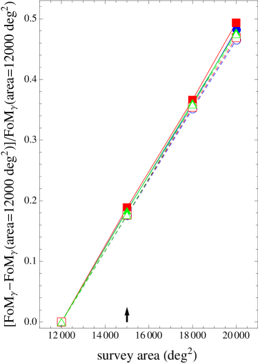
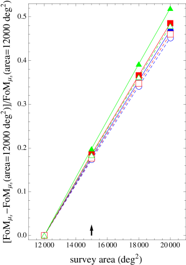
In Figure 12 we show the dependence of the FoMs for and (left and right panels respectively) on the area - galaxy number density. In order to better appreciate the functional behaviour, we plot the relative improvement in the FoM when varying the area with respect to the FoM of area : . Here we can see that the improvement in the growth measurement is nearly linear, at least for the area interval considered (), and mildly dependent on the dark energy model considered, but also rather slow, so that a large increase in area might not be favoured in case the cost for obtaining it grows too fast. Comparing left to right plot, we also note that in the case of the parameterisation the improvement of the FoM depends more strongly on the cosmological model one has previously assumed. The largest improvement appears for flat CPL.
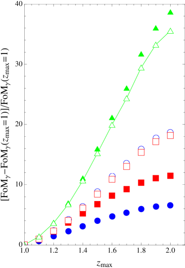
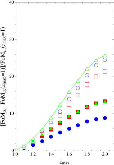
As regards the dependence of the FoM on , we evaluated it by calculating our total Fisher matrix as the sum of the Fisher matrices computed for the redshift bins from to only (see Sec. 3 for further details on the general Fisher matrix calculation technique). Fig. 13 shows the relative difference of the FoM() to the FoM for : . Here the amplitude of the spread due to model assumptions is much wider than for the area - galaxy number density dependence, and wider in the case of . The latter is because the derivative of our observable with respect to decreases with redshift while its derivative with respect to increases (as we have checked numerically), so that at is more sensitive to changes in than in . This explains why in the case of and for the CPL model, which has the strongest time-dependence of the background cosmology, there is more advantage from higher redshift bins than for the case of . In both parameterisations complex models gain more from higher redshift data, so e.g. by increasing wCDM’s FoM improves more than qLCDM’s does, and the FoM of models with improves more than the corresponding one for flat models (with the exception of CPL with ). In the case of , this is easy to explain. We know that . In the case of a flat qLCDM model approaches as soon as matter starts dominating, and this happens already for small values of . From such on, the value of becomes practically independent of so that higher redshift data do not help constraining it anymore. If instead the model is more complex, e.g. is allowed to vary away from , then at larger so that increasing improves more the FoM. Something similar also likely happens for , but it is more difficult to illustrate it since we only have numerical solutions for in this case. Note also that for there is more difference between curved and flat models than for .
This and the fact that the FoM grows rapidly when increasing encourages the effort to reach the highest possible maximum limiting redshift in future surveys.
Finally, we test the dependence of the growth FoM on the redshift interval covered by the survey. We plot in Figure 14 contours of constant FoM (in particular, , , and of the maximum FoM reached in each case) as functions of and , where varies between and and between and . We concentrate here only on CPL dark energy, since this is the most complex and complete of our set of models. We first note that for the parameterisation there is stronger dependence on curvature of the FoM than for the parameterisation (compare solid and dashed lines).
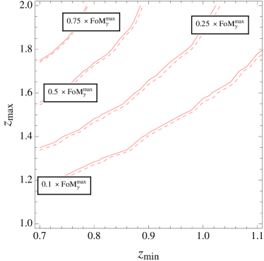
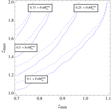
We also note that the contours for and have different shapes. Let us consider a specific example. If we look at , we need a to reach of the maximum FoM, for both parameterisations. For other values of , the two parameterisations give different indications. For (), the minimum value of required in order to obtain of the maximum achievable FoM is larger (smaller) for than for . This study is warning us against optimising an experiment on the base of one parameterisation only. In the absence of a clear preference for one parameterisation over the other, an operative way to proceed in this particular case would be to choose the most conservative and limits, for which the desired FoM is achieved in both parameterisations.
To end this section on figures of merit, we list in Table 5 and 6 the FoMs, reached using the maximum available redshift range for all combinations of cosmological models, both for the and the parameterisation. We also look at how the FoM is improved when adding data from a low- galaxy survey (as may be BOSS) and further add Planck data. In square brackets we show how the FoMs are degraded in the pessimistic case of the galaxy number density being half that forecasted in Geach et al. (2008).
| Euclid | + low-z data | + Planck | |||
|---|---|---|---|---|---|
| flat space | curved space | flat space | curved space | curved space | |
| qLCDM | 545 [361] | 209 [135] | 561 [376] | 221 [137] | |
| wCDM | 217 [146] | 74 [48] | 225 [153] | 75 [49] | |
| CPL | 35 [23] | 30 [20] | 35 [23] | 30 [20] | 141 [140] |
| Euclid | + low-z data | + Planck | |||
|---|---|---|---|---|---|
| flat space | curved space | flat space | curved space | curved space | |
| qLCDM | 244 [159] | 93 [59] | 251 [165] | 94 [60] | |
| wCDM | 82 [55] | 28 [18] | 85 [58] | 29 [18] | |
| CPL | 18 [13] | 9 [6] | 19 [13] | 9 [6] | 82 [82] |
7 Distinguishing General Relativity from modified gravity models
We finally turn to trying and answering the question “is the Euclid spectroscopic survey able to distinguish between GR and modified gravity?” To do this we use model selection tools (aimed precisely at telling how strongly a set of data prefers a model over other models) from Bayesian statistics. In particular, we apply the method of Heavens et al. (2007), where the Fisher matrix approach is generalised to the context of model selection. The Bayesian tool for model selection is the Bayes’ factor , defined as the ratio of probabilities of model to model , given the same data , independently of the values assumed by the model parameters or :
| (8) |
where is the probability of model given the data , is the prior probability of model (i.e. the probability that model is true before the experiment is done), which is unknown, and we will assume ; is what is usually called the likelihood function (i.e. the probability that the data are true given the model with parameters ); is the prior probability of the model parameters (i.e. the probability distribution that one believes the model parameters have before the experiment is done). As in Heavens et al. (2007), is here a dark energy model well described by the CPL parameterisation, while is a modified gravity model whose background expansion can still be described by the same of the CPL parameterisation, (not necessarily by the same fiducial parameters) but now the growth index is fixed to a fiducial value different from the GR value of . Our fiducial cosmology is that of Eqs. (5). For our case the forecasted Bayes’ factor is (Heavens et al., 2007)
| (9) |
where corresponds to a uniform prior on , and are the Fisher matrices for GR and the modified gravity model, respectively, and represent the shifts of the parameters of due to a shift in from the fiducial value :
| (10) |
for corresponding to all parameters but , while for associated to the parameter. Here is the vector drawn from by extracting the column corresponding to the parameter and the rows corresponding to all parameters except . From the above we see that depends on the offset of with respect to the GR value, , and on the prior on , .
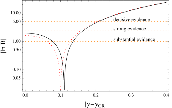
In Figure 15 we show the dependence of the log of on for two different priors (represented by the solid and red dashed lines) in the case of our Euclid-like spectroscopic galaxy survey. The horizontal dotted lines describe values of which correspond to ’substantial’ (), ’strong’ () and ’decisive’ () evidence in favour of one model with respect to the other (bottom to top) according to Jeffreys’ scale (Jeffreys, 1998). As can be seen from the figure, the Euclid spectroscopic survey alone will be able to substantially distinguish between GR and a modified gravity model if , while it will be able to decisively distinguish between models if . We have also computed the evidence using the parameterisation, with uniform prior distributions in the interval and . For both priors it results that with Euclid spectroscopic data alone ’substantial’ (’strong’) evidence can be obtained in favour of a modified gravity if the latter has (). The addition of the weak lensing data from the Euclid photometric survey is expected to improve these results considerably.
8 Conclusions
In this paper we have investigated how strongly the Euclid galaxy spectroscopic survey in the current reference configuration can constrain the growth of structure and consequently how well it can differentiate a GR cosmology from alternatives to it.
We have found that we can reach precisions between and in the measurement of depending on the redshift bin, where the highest precision is reached for .
Comparing the Euclid spectroscopic survey with other ongoing and future galaxy redshift surveys we note that Euclid will reach the highest precision in the growth rate measurement. Euclid will be perfectly complementary to BOSS and BigBOSS: the three surveys together will allow to cover an extremely large redshift range: .
This precision in translates into a precision in the measurement of the growth index which depends on the specific background cosmology adopted. We have obtained marginalised errors on (or ) between and . The parameterisation of the growth rate we have adopted is (for curved space, ), where a departure from GR is represented by a deviation of from . We have considered nested background models: qLCDM (a model with constant ), wCDM and CPL, both flat and curved.
We have compared the relative gain in growth FoM (quantifying the precision in the joint measurement of and ) for two different growth parameterisations, being the already mentioned and the parameter (Pogosian et al., 2010; Song et al., 2011). We have found that when increasing the survey area (and correspondingly reducing the galaxy number density, having fixed the total observing time) the FoM grows linearly. Moreover, this growth is quite mild.
The relative gain in FoM when increasing is large, both using and . We also have noted that (for curved models) the relative improvement increasing is approximately linear, encouraging the effort to reach the maximum possible limiting redshift. We then have examined the dependence of the FoM on the redshift interval covered by the survey. From Fig. 14 it is possible to notice that to reach a desired FoM improvement one needs lower (or higher ) when considering than when choosing . This warns us against relying on one parameterisation only when optimising an experiment.
Finally we have forecasted the Bayesian evidence for Euclid and found that the spectroscopic survey alone will be able to substantially (decisively) distinguish between GR and modified gravity models having (). This result is expected to improve even further when adding data from the photometric survey of Euclid, which improve noticeably the precision in the measurement of (see e.g. Fig.2.5 of Laureijs et al. 2011).
Acknowledgements
We wish to thank Domenico Sapone for essential and kind help in developing the Fisher code, Cinzia Di Porto for kindly providing details on coupled models, Ben Granett, Matteo Chiesa, Davide Bianchi and Alida Marchetti for enlightening discussions. EM was supported by INAF through PRIN 2007, by the Spanish MICINNs Juan de la Cierva programme (JCI-2010-08112), by CICYT through the project FPA-2009 09017, by the Community of Madrid through the project HEPHACOS (S2009/ESP-1473) under grant P-ESP-00346 and by the European Union FP7 ITN INVISIBLES (Marie Curie Actions, PITN- GA-2011- 289442). WJP is grateful for support from the UK Science and Technology Facilities Council (STFC). LS is grateful for support from the Georgian National Science Foundation grant GNSF ST08/4-442 and SNFS SCOPES grant no. 128040. LS and WJP are grateful for support from the European Research Council (ERC). YW was supported in part by DOE grant DE-FG02-04ER41305. CC acknowledges PRIN MIUR “Dark energy and cosmology with large galaxy surveys”. EM, LG, BG, PF, ER, AC, CC, NR and GZ acknowledge support from ASI Euclid-NIS I/039/10/0 grants.
References
- Acquaviva et al. (2008) Acquaviva V., Hajian A., Spergel D. N., Das S., 2008, Phys. Rev., D78, 043514
- Albrecht et al. (2006) Albrecht A., et al., 2006, astro-ph/0609591
- Alcock & Paczynski (1979) Alcock C., Paczynski B., 1979, Nature, 281, 358
- Amendola (1999) Amendola L., 1999, Phys. Rev., D60, 043501
- Amendola et al. (2008) Amendola L., Kunz M., Sapone D., 2008, JCAP, 0804, 013
- Amendola et al. (2005) Amendola L., Quercellini C., Giallongo E., 2005, Mon. Not. Roy. Astron. Soc., 357, 429
- Amendola & Tsujikawa (2008) Amendola L., Tsujikawa S., 2008, Phys. Lett., B660, 125
- Amendola & Tsujikawa (2010) Amendola L., Tsujikawa S., 2010, Dark Energy: Theory and Observations. Cambridge University Press
- Bartolo & Pietroni (2000) Bartolo N., Pietroni M., 2000, Phys. Rev., D61, 023518
- Bassett et al. (2009) Bassett B. A., Fantaye Y., Hlozek R., Kotze J., 2009, 0906.0993
- Bassett et al. (2005) Bassett B. A., Parkinson D., Nichol R. C., 2005, Astrophys.J., 626, L1
- Belloso et al. (2011) Belloso A. B., Garcia-Bellido J., Sapone D., 2011, JCAP, 1110, 010
- Bianchi et al. (2012) Bianchi D., et al., 2012, arXiv:1203.1545
- Blake et al. (2011) Blake C., et al., 2011, Mon. Not. Roy. Astron. Soc., 415, 2876
- Cabre & Gaztanaga (2009) Cabre A., Gaztanaga E., 2009, Mon. Not. Roy. Astron. Soc., 393, 1183
- Capozziello (2002) Capozziello S., 2002, Int. J. Mod. Phys., D11, 483
- Capozziello et al. (2003) Capozziello S., Cardone V. F., Carloni S., Troisi A., 2003, Int. J. Mod. Phys., D12, 1969
- Carroll et al. (2004) Carroll S. M., Duvvuri V., Trodden M., Turner M. S., 2004, Phys. Rev., D70, 043528
- Chevallier & Polarski (2001) Chevallier M., Polarski D., 2001, Int. J. Mod. Phys., D10, 213
- Chiba (1999) Chiba T., 1999, Phys. Rev., D60, 083508
- Cimatti et al. (2009) Cimatti A., et al., 2009, Exper. Astron., 23, 39
- Cole et al. (2005) Cole S., et al., 2005, Mon. Not. Roy. Astron. Soc., 362, 505
- Copeland et al. (2006) Copeland E. J., Sami M., Tsujikawa S., 2006, Int. J. Mod. Phys., D15, 1753
- da Angela et al. (2008) da Angela J., et al., 2008, Mon. Not. Roy. Astron. Soc., 383, 565
- Di Porto & Amendola (2008) Di Porto C., Amendola L., 2008, Phys. Rev., D77, 083508
- Di Porto et al. (2011) Di Porto C., Amendola L., Branchini E., 2011, arXiv:1101.2453
- Drinkwater et al. (2010) Drinkwater M. J., et al., 2010, Mon. Not. Roy. Astron. Soc., 401, 1429
- Dvali et al. (2000) Dvali G. R., Gabadadze G., Porrati M., 2000, Phys. Lett., B485, 208
- Eisenstein et al. (2005) Eisenstein D. J., et al., 2005, Astrophys. J., 633, 560
- Frieman et al. (2008) Frieman J., Turner M., Huterer D., 2008, Ann. Rev. Astron. Astrophys., 46, 385
- Fry (1985) Fry J. N., 1985, Phys. Lett., B158, 211
- Gannouji et al. (2009) Gannouji R., Moraes B., Polarski D., 2009, JCAP, 0902, 034
- Garilli et al. (2010) Garilli B., Fumana M., Franzetti P., Paioro L., Scodeggio M., Le Fèvre O., Paltani S., Scaramella R., 2010, PASP, 122, 827
- Geach et al. (2008) Geach J. E., et al., 2008, Mon. Not. Roy. Astron. Soc., 388, 1473
- Gong et al. (2009) Gong Y., Ishak M., Wang A., 2009, Phys. Rev., D80, 023002
- Guzzo et al. (2008) Guzzo L., et al., 2008, Nature, 451, 541
- Hamilton (1998) Hamilton A., 1998, The Evolving Universe. Vol. 321 of Astrophysics and Space Science Library, Kluwer Academic Publishers
- Hawkins et al. (2003) Hawkins E., et al., 2003, Mon. Not. Roy. Astron. Soc., 346, 78
- Heath (1977) Heath D. J., 1977, Mon. Not. Roy. Astron. Soc., 179, 351
- Heavens et al. (2007) Heavens A. F., Kitching T. D., Verde L., 2007, Mon. Not. Roy. Astron. Soc., 380, 1029
- Ilbert et al. (2009) Ilbert O., Capak P., Salvato M., Aussel H., McCracken H., et al., 2009, Astrophys.J., 690, 1236
- Ishak & Dossett (2009) Ishak M., Dossett J., 2009, Phys. Rev., D80, 043004
- Jeffreys (1998) Jeffreys H., 1998, The Theory of Probability, third edn. Oxford University Press
- Kaiser (1987) Kaiser N., 1987, Mon. Not. Roy. Astron. Soc., 227, 1
- Kazin et al. (2010) Kazin E. A., et al., 2010, Astrophys.J., 710, 1444
- Kobayashi (2010) Kobayashi T., 2010, Phys. Rev., D81, 103533
- Komatsu et al. (2009) Komatsu E., et al., 2009, Astrophys. J. Suppl., 180, 330
- Komatsu et al. (2011) Komatsu E., et al., 2011, Astrophys.J.Suppl., 192, 18
- Koyama & Maartens (2006) Koyama K., Maartens R., 2006, JCAP, 0601, 016
- Kunz & Sapone (2007) Kunz M., Sapone D., 2007, Phys. Rev. Lett., 98, 121301
- Lahav et al. (2002) Lahav O., et al., 2002, Mon. Not. Roy. Astron. Soc., 333, 961
- Lahav et al. (1991) Lahav O., Lilje P. B., Primack J. R., Rees M. J., 1991, Mon. Not. Roy. Astron. Soc., 251, 128
- Laureijs (2009) Laureijs R., 2009, arXiv:0912.0914
- Laureijs et al. (2011) Laureijs R., Amiaux J., Arduini S., Augueres J.-L., Brinchmann J., et al., 2011, arXiv:1110.3193
- Lewis et al. (2000) Lewis A., Challinor A., Lasenby A., 2000, Astrophys. J., 538, 473
- Lightman & Schechter (1990) Lightman A. P., Schechter P. L., 1990, Astrophys. J. Suppl., 74, 831
- Linder (2003) Linder E. V., 2003, Phys. Rev. Lett., 90, 091301
- Linder (2005) Linder E. V., 2005, Phys. Rev., D72, 043529
- Linder (2008) Linder E. V., 2008, Astropart. Phys., 29, 336
- Linder & Cahn (2007) Linder E. V., Cahn R. N., 2007, Astropart. Phys., 28, 481
- Lue et al. (2004) Lue A., Scoccimarro R., Starkman G. D., 2004, Phys. Rev., D69, 124015
- Maartens (2007) Maartens R., 2007, J. Phys. Conf. Ser., 68, 012046
- Martel (1991) Martel H., 1991, Astrophys. J., 377, 7
- Motohashi et al. (2010) Motohashi H., Starobinsky A. A., Yokoyama J., 2010, arXiv:1002.0462
- Nesseris & Perivolaropoulos (2008) Nesseris S., Perivolaropoulos L., 2008, Phys. Rev., D77, 023504
- Orsi et al. (2009) Orsi A., et al., 2009, Mon. Not. Roy. Astron. Soc., 405, 1006
- Peebles (1980) Peebles P., 1980, The Large Scale Structure of the Universe. Princeton University Press, Princeton, New Jersey
- Percival & White (2009) Percival W. J., White M., 2009, Mon. Not. Roy. Astron. Soc., 393, 297
- Perrotta et al. (2000) Perrotta F., Baccigalupi C., Matarrese S., 2000, Phys. Rev., D61, 023507
- Pogosian et al. (2010) Pogosian L., Silvestri A., Koyama K., Zhao G.-B., 2010, Phys. Rev., D81, 104023
- Polarski (2006) Polarski D., 2006, AIP Conf. Proc., 861, 1013
- Reid et al. (2010) Reid B. A., et al., 2010, Mon. Not. Roy. Astron. Soc., 404, 60
- Ross et al. (2007) Ross N. P., da Ângela J., Shanks T., Wake D. A., Cannon R. D., Edge A. C., Nichol R. C., Outram P. J., Colless M., Couch W. J., Croom S. M., de Propris R., Drinkwater M. J., Eisenstein D. J., Loveday J., Pimbblet K. A., Roseboom I. G., Schneider D. P., Sharp R. G., Weilbacher P. M., 2007, Mon. Not. Roy. Astron. Soc., 381, 573
- Samushia et al. (2011) Samushia L., et al., 2011, Mon. Not. Roy. Astron. Soc., 410, 1993
- Samushia et al. (2011) Samushia L., Percival W. J., Raccanelli A., 2011, arXiv:1102.1014
- Sapone & Amendola (2007) Sapone D., Amendola L., 2007, arXiv:0709.2792
- Schlegel et al. (2011) Schlegel D., et al., 2011, arXiv:1106.1706
- Schlegel et al. (2009) Schlegel D., White M., Eisenstein D., 2009, arXiv:0902.4680
- Seo & Eisenstein (2003) Seo H.-J., Eisenstein D. J., 2003, Astrophys. J., 598, 720
- Simpson & Peacock (2010) Simpson F., Peacock J. A., 2010, Phys. Rev., D81, 043512
- Song et al. (2011) Song Y.-S., et al., 2011, Phys. Rev., D84, 083523
- Song & Percival (2009) Song Y.-S., Percival W. J., 2009, JCAP, 0910, 004
- Tauber et al. (2010) Tauber J. A., Mandolesi N., Puget J.-L., Banos T., Bersanelli M., Bouchet F. R., Butler R. C., Charra J., Crone G., Dodsworth J., et al. 2010, Astron. Astrophys., 520, A1+
- Tegmark (1997) Tegmark M., 1997, Phys. Rev. Lett., 79, 3806
- Tsujikawa (2007) Tsujikawa S., 2007, Phys. Rev., D76, 023514
- Tsujikawa et al. (2009) Tsujikawa S., Gannouji R., Moraes B., Polarski D., 2009, Phys. Rev., D80, 084044
- Uzan (1999) Uzan J.-P., 1999, Phys. Rev., D59, 123510
- Wang & Steinhardt (1998) Wang L.-M., Steinhardt P. J., 1998, Astrophys. J., 508, 483
- Wang (2008) Wang Y., 2008, JCAP, 0805, 021
- Wang et al. (2010) Wang Y., et al., 2010, Mon. Not. Roy. Astron. Soc., 409, 737
- Wei (2008) Wei H., 2008, Phys. Lett., B664, 1
- White et al. (2011) White M., et al., 2011, Astrophys. J., 728, 126
- White et al. (2008a) White M., Song Y.-S., Percival W. J., 2008a, Mon. Not. Roy. Astron. Soc., 397, 1348
- White et al. (2008b) White M., Song Y.-S., Percival W. J., 2008b, Mon. Not. Roy. Astron. Soc., 397, 1348
- Zehavi et al. (2005) Zehavi I., et al., 2005, Astrophys. J., 621, 22
- Ziaeepour (2011) Ziaeepour H., 2011, arXiv:1112.6025
Appendix A Growth of structures
In a Friedmann-Lemaitre-Robertson-Walker (FLRW) universe, the growth of linear perturbations is described by the perturbed Einstein equations and conservation of the energy-momentum tensor equations. If we consider scalar perturbations about a FLRW background in the Newtonian gauge, in Fourier space and in the limit of small scales, an equation for the growth rate can be derived:
| (11) |
A solution for has now to be found and depends on the form of .
A.1 Parameterisations of growth in GR and deviations from it: a constant growth index
A.1.1 Flat LCDM and quintessence
If we assume a flat model with a simple cosmological constant or a dark energy with (quasi) constant equation of state , with Friedmann equation , then it is possible to find a good solution of Eq. (11) by assuming
| (12) |
where the growth index is a constant. This was first proposed by Peebles (1980) for a matter-dominated universe at , with . A better approximation for the same model was found by Fry (1985) and Lightman & Schechter (1990), with . For the case of LCDM, is a very good approximation, at least in the redshift range of interest here. As shown in Wang & Steinhardt (1998), if we consider, instead of a standard cosmological constant, a quintessence field with slowly varying , then is still a good approximation, since the correction term has a weak dependence on if this is close enough to .
For larger redshift ranges, from to today, and demanding a very high precision, a different solution for LCDM was proposed by Ishak & Dossett (2009). For models with non-slowly varying , Linder & Cahn (2007) and Linder (2005) propose different parameterisations.
We restrict ourselves to models with slowly varying and decide not to use the large redshift range parameterisation since we do not require an accuracy that high. Instead, we are interested in parameterisations for models where curvature is present, since this parameter has been shown to be degenerate with dark energy and we wish to explore it in a consistent way.
A.1.2 Generalisation to curved LCDM and quintessence
In the case of a curved LCDM model, the first attempts at modelling were proposed by Martel (1991) and Lahav et al. (1991).
More recently, in Gong et al. (2009), two possible approaches are suggested. The first (less accurate) approach consists in still assuming , but changing the form of . The second consists in taking (with ).
In the second case, which is found to be more accurate, the solution is
| (13) |
We use the parameterisation (13) for our forecasts.
A.1.3 Modified gravity: the case of DGP, gravity and scalar-tensor theories
A parameterisation as that of Eq. (12) or (13) is valid also for some modified gravity models (see Amendola & Tsujikawa 2010 for a complete review of viable alternatives to GR), when taking a different fiducial .
Let us first take the DGP model. For flat space, Linder & Cahn (2007) showed that the growth rate is still well parameterised by Eq. (12) with a constant . Wei (2008) and Gong et al. (2009) derived the expected value of by solving the modified growth equations of Lue et al. (2004); Koyama & Maartens (2006): . A constant still fits the curve well enough (Linder & Cahn, 2007). If we include curvature, we can proceed, following Gong et al. (2009), as for curved quintessence, e.g. parameterising as in Eq. (13), and we find that the best fitting is again .
Instead of adding extra dimensions, it is possible to modify gravity in four dimensions. This is done e.g. in theories (Capozziello, 2002; Capozziello et al., 2003; Carroll et al., 2004), where the Einstein-Hilbert Lagrangian density is modified into a different function, . The function is strongly constrained by local gravity tests (Amendola & Tsujikawa, 2008), nevertheless the phenomenology of the growth of structure for these models is still very rich. Their growth index is in general time- and scale-dependent (Tsujikawa, 2007; Gannouji et al., 2009; Tsujikawa et al., 2009; Motohashi et al., 2010). As found in Tsujikawa et al. (2009) and Gannouji et al. (2009), the importance of scale-dependent dispersion of depends on the particular model chosen and on its parameters. For some particular values of the parameters, there can be scale-independent growth. We do not consider scale dependence in this work, although it would be very interesting to examine this feature, as it might be a smoking gun for models (Pogosian et al., 2010). Time dependence can arise in general. Forecasts on for Euclid-like galaxy redshift surveys have been computed in Di Porto et al. (2011) and we refer the reader to this paper for a full analysis of the topic. In this work we concentrate on a constant , which somehow corresponds to a averaged over the redshift range of the survey, weighted by the error on in each redshift bin. Given that viable models show a lower growth index with respect to GR, becoming even smaller at higher , if one was to detect an unusually low averaged constant , this would point to models. The use of a time and possibly scale dependent could then in principle allow to distinguish among different models.
Scalar-tensor theories (Amendola, 1999; Uzan, 1999; Chiba, 1999; Bartolo & Pietroni, 2000; Perrotta et al., 2000) are a generalisation of models, where the Lagrangian density is . Given the generality of these theories, the phenomenology of their growth of structure is very rich. The growth of matter perturbations in some of these models has been studied e.g. in Di Porto & Amendola (2008); Gannouji et al. (2009); Kobayashi (2010). In general depends on time (and scale), but there are also specific cases where for redshifts (Kobayashi, 2010).
A.2 Parameterisations of growth in GR and deviations from it: physical parameters
Instead of parameterising the deviation from GR with , we can use a different approach, proposed by Amendola et al. (2008). This consists in directly parameterising the full Einstein equations instead of some already approximated version of them (e.g for small scales). This approach may turn useful when combining constraints from different observational tools, which might need different approximations. This way, the parameters would always have a physical meaning and one would avoid difficulties in interpreting results, as pointed out very neatly in Pogosian et al. (2010). It is precisely the parameterisation proposed in Pogosian et al. (2010) that we use and compare to . The Einstein equations defining the parameterisation are:
| (14) |
where and are the metric perturbations in the Newtonian gauge:
| (15) |
Since the galaxy power spectrum is sensitive to and not to the anisotropic stress (which depends on the difference between the two potentials and ), the parameter is sufficient for our work and we do not use at all.
For simplicity, we decide to assume again scale-independence: (although see Pogosian et al. 2010 and Sec. A.1.3 for reasons to keep scale-dependence). We model as in Song et al. (2011):
| (16) |
which is motivated by DGP and reduces to GR for . So, using again the function defined previously, we obtain
| (17) |
We can solve this equation numerically, by imposing the initial condition at an initial redshift of matter domination : (where can be determined from Eq. (32) of Pogosian et al. (2010)).
Appendix B Predictions using the parameterisation
Here we present forecasts on the marginalised errors on cosmological parameters when, instead of using , the alternative parameterisation is used (see Appendix A.2).
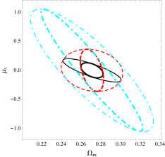
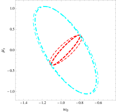
As we can see from Figs. 16 and 17, with Euclid spectroscopic data alone the absolute marginalised error on and or will be .
