Competition between superconductivity and nematic order in high-$T_{c}$ superconductor

Abstract

We investigate the competition between $d$-wave superconductivity and nematic order in high-$T_{c}$ superconductor, and examine the role played by gapless fermionic degrees of freedom. Apart from the competitive interaction with the superconducting order parameter, the nematic order parameter couples strongly to gapless nodal quasiparticles. The interplay of these two kinds of interactions is analyzed by means of renormalization group method. In case the fermionic degree of freedom are entirely neglected, the competitive interaction between two bosonic order parameters is strongly relevant, and can lead to runaway behavior. However, these properties are fundamentally changed once the dynamics of fermions are taken into account. At the nematic quantum critical point where an extreme fermion velocity anisotropy occurs, the superconducting and nematic order parameters are decoupled from each other. Consequently, the phase transitions are continuous, and $d$-wave superconductivity can coexist with nematic order homogeneously. These results indicate that the gapless fermions can play an important role and should be carefully included in the theoretical description of competing orders.

1 Introduction

Unconventional superconductors usually refer to the superconductors those can not be understood within the conventional Bardeen-Cooper-Schrieffer (BCS) theory. Notable examples of unconventional superconductors are high-$T_{c}$ cuprate superconductor, heavy fermion superconductor, and iron-based superconductor. Unlike BCS superconductors, unconventional superconductivity is generally driven by electron-electron interactions, and often has a magnetic origin. Another interesting property of unconventional superconductor is that its ground state is not unique. In addition to the defining superconducting state, unconventional superconductors also exhibit a variety of other symmetry-broken ground states, including antiferromagnetc, nematic, and stripe states, upon tuning such parameters as doping and pressure [1, 2, 3, 4, 5]. A widely recognized notion is that the long-range superconducting order competes, and under certain circumstances coexists, with other long-range orders. The competition and possible coexistence between different orders can give rise to rich properties, and hence have attracted intense theoretical and experimental interest in the past years.

The successful microscopic theory of competing orders has not yet been established to date, primarily because the pairing mechanism in most unconventional superconductors is still undetermined. A realistic and commonly used strategy is to build low-energy effective field theory on phenomenological grounds. One can first write down the Ginzburg-Landau (GL) actions for two bosonic order parameters and then introduce certain coupling terms between these two scalar fields. Such generalized GL model has recently been applied to describe competing orders in a number of unconventional superconductors [6, 8, 7, 13, 14, 10, 11, 9, 15, 12]. An early success of such theoretical investigation is the prediction of field-induced antiferromagnetic core in the supercondcuting vortices of high-$T_{c}$ superconductors [6]. This prediction was subsequently confirmed in experiments [16, 17]. Interestingly, experiments further found that the antiferromagnetic order not only exists in the vortex cores, but also extends into the superconducting region [16] and exhibits nontrivial spatial modulation [17, 18]. A phenomenological field theory that contains a simple quadratic-quadratic coupling term between superconducting and antiferromagnetic order parameters was put forward to understand these new findings [7, 8].

Recently, the issue of competing orders has attracted revived interest. It is found that the competitive interaction between distinct orders can drive an instability, which gives rise to a general tendency of first order transition [14, 11]. This phenomenon may account for the first order transition observed in some unconventional superconductors [4]. In addition, nonuniform glassy electronic phases and Brazovskii type transitions are predicted to emerge due to competition between two long-range orders [10]. Another interesting observation is that the competition between superconducting and antiferromagnetic orders can help to judge the gap symmetry of iron-based superconductors [9, 12]. Furthermore, the competition between superconducting and nematic orders might be responsible for [15] the electronic anisotropy observed in the vortex state of FeSe superconductor [19].

The effective field theory adopted in previous analysis of competing orders normally contains only two bosonic order parameters. The fermionic degrees of freedom are usually completely integrated out in the spirit of Hertz-Millis-Moriya (HMM) theory [20, 21, 22]. This integration procedure is expected to be applicable in systems that do not contain gapless fermionic excitations. For instance, the iron-based superconductors seem to have a $s$-wave energy gap, so the electronic excitations are fully gapped and can be safely integrated out [9, 12]. However, such integration manipulation is not always valid. Indeed, its validity has recently been questioned in several itinerant electron systems [23, 25, 24, 26]. In the systems that exhibit gapless fermionic excitations, integrating out fermions may lead to singularities, especially in the vicinity of quantum critical point (QCP). Actually, infrared singularities have been found on the border of several quantum phase transitions [23, 24, 25, 26]. In order to properly describe the quantum critical behavior in these systems, it is more appropriate to maintain both bosonic order parameter and gapless fermions in the effective theory. When a long-range order competing with superconductivity also couples to gapless fermions, it would be interesting to go beyond HMM theory and examine the role of gapless fermions. Recent analysis presented in Refs. [13, 27] did suggest nontrivial roles played by gapless fermions.

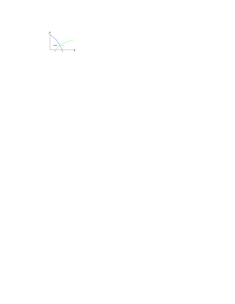
Figure 1: Schematic phase diagram on $(x,T)$-plane of high-$T_{c}$ superconductors. $x$ represents doping concentration. $x_{1}$ and $x_{2}$ are QCPs of superconducting and nematic phase transitions, repectively.

In various types of superconductors, superconductivity may compete with several possible long-range orders. To examine the role of fermions, we wish to study a prototypical model which describes competition between two distinct long-range orders, contains gapless fermions, and in the meantime is technically controllable. In the present paper, we choose to consider the competition between superconductivity and nematic order in the contexts of high-$T_{c}$ superconductors. In recent years, there has been increasing experimental evidence pointing towards the existence of an electronic nematic phase in some high-$T_{c}$ superconductors [1, 3, 2, 28, 29, 30, 31], especially YBa₂Cu₃O_6+δ and Bi₂Sr₂CaCu₂O_8+δ. According to these experiments, a nematic order is predicted to compete and coexist with superconductivity, which is schematically plotted in Fig. 1. The nematic transition and the coupling of nematic order to gapless fermions have stimulated intense research effort [1, 3, 2, 32, 35, 38, 33, 34, 36, 37, 39, 40, 41, 42, 27]. From a field-theoretic viewpoint, the nematic order parameter is a real scalar field and does not carry a finite wave vector, which substantially simplifies theoretical calculations.

It is known that high-$T_{c}$ superconductor has a $d_{x^{2}-y^{2}}$ energy gap, which vanishes at four nodes, $\left(\pm\frac{\pi}{2},\pm\frac{\pi}{2}\right)$. Therefore, gapless nodal quasiparticles (qps) are present even at the lowest energy in the superconducting phase. These nodal qps are believed to be responsible for many anomalous low-temperature properties of the superconducting dome. When a nematic QCP exists somewhere in the superconducting dome, as shown in Fig. 1, the fluctuation of nematic order parameter couples to gapless nodal qps. This coupling can generate non-Fermi liquid behaviors and other anomalous phenomena in the vicinity of nematic QCP [36, 37, 40, 39, 41, 42, 27]. In particular, the ratio $\kappa$ between gap velocity $v_{\Delta}$ and Fermi velocity $v_{F}$ of nodal qps is driven to vanish, i.e., $\kappa=v_{\Delta}/v_{F}\rightarrow 0$, by the critical nematic fluctuation [37], leading to extreme velocity anisotropy. These unusual behaviors may have significant effects on the interplay between superconductivity and nematic order, which is the topic of this paper.

In this paper, we first write down an effective field theory that describes both the competitive interaction between two bosonic (superconducting and nematic) order parameters and the Yukawa-type coupling between nematic order parameter and nodal qps. We then carry out a detailed renormalization group (RG) analysis [43] within this effective theory. Specifically, we will derive and solve the RG flow equations of all physical parameters so as to determine the possible stable fixed points. We will demonstrate that gapless fermionic degrees of freedom can fundamentally change the basic properties of the interplay between superconductivity and nematic order. In case all the fermions are entirely neglected, the ordering competition may be strong enough to produce runaway behavior and turn continuous phase transitions to first order [14]. However, once the dynamics of gapless nodal qps are properly incorporated, a stable fixed point exists with the two originally competing bosonic order parameters decoupled from each other in the vicinity of nematic QCP. As a result, both the superconducting and nematic transitions remain continuous. In addition, the d-wave superconductivity can coexist with the nematic order homogeneously. Our results indicate that it is important to include the dynamics of gapless fermions in the theoretic description of competing orders.

In Sec. 2, we write down the effective action which contains two bosonic order parameters and gapless nodal qps. In Sec. 3, we make RG calculations and derive the flow equations for all parameters in the effective action. In Sec. 4, we present numerical solutions of the flow equations and discuss the physical implications. The paper is ended in Sec. 5 with summary and conclusion.

2 Effective field theory of competing orders

We first need to write down an effective field theory to describe the competition between superconducting and nematic orders. This will be done largely on phenomenological grounds. In the phase diagram presented in Fig. 1, the horizonal axe is doping concentration $x$. The QCP of superconducting transition is $x_{1}$, which is roughly $x_{1}\approx 0.05$ in many high-$T_{c}$ superconductors. The anticipated QCP for nematic transition is represented by $x_{2}$. So far, the precise value, and even the very existence, of $x_{2}$ have not yet been unambiguously determined. Here, we assume that $x_{2}$ is larger than $x_{1}$, which implies a bulk coexistence of superconducting and nematic orders.

In the present system, there are three types of degrees of freedom: superconducting order parameter $\psi$, nematic order parameter $\phi$, and gapless nodal qps $\Psi$. The competition between superconducting and nematic orders can be described by a repulsive quadratic-quadratic coupling term, $\propto\psi^{2}\phi^{2}$, which is widely adopted in the description of competing orders [12, 13, 14, 27]. In addition to this competitive interaction, the nematic order parameter $\phi$ also interacts with gapless nodal qps $\Psi$, which is usually described by a Yukawa-type coupling term. There is, however, no direct coupling between the superconducting order parameter and nodal qps. First, the nodal qps are excited from the $d_{x^{2}-y^{2}}$ gap nodes where superconducting order parameter vanishes. Second, these qps are known to have a sharp peak and a very long lifetime in the superconducting dome in the absence of competing orders [44], so their coupling to $\psi$ must be quite weak. Furthermore, in this paper we are mainly interested in the physical properties in the close vicinity of nematic QCP $x_{2}$, where the fluctuation of nematic order parameter is critical. Unless the superconducting QCP $x_{1}$ coincides with, or is very close to, $x_{2}$, the fluctuation of superconducting order parameter is not critical at $x_{2}$. Therefore, the coupling between superconducting order parameter and nodal qps is not as important as that between critical nematic fluctuation and nodal qps at $x_{2}$, and can be simply neglected.

On the basis of the above qualitative analysis, we can write down the following partition function

$$Z = \int\mathcal{D}\psi\mathcal{D}\phi\mathcal{D}\bar{\Psi}\mathcal{D}\Psi e^{S},$$ (1)

where the effective action is

$$S = S_{\psi}+S_{\phi}+S_{\Psi}+S_{\psi\phi}+S_{\Psi\phi},$$ (2)

$$S_{\psi} = \frac{1}{2}\int\frac{d^{3}q}{(2\pi)^{3}}(-2\alpha+q^{2})\psi^{2}+\frac{\beta}{2}\int d^{2}\mathbf{r}d\tau\psi^{4},$$ (3)

$$S_{\phi} = \frac{1}{2}\int\frac{d^{3}q}{(2\pi)^{3}}\left(-2r+q^{2}\right)\phi^{2}+\frac{u}{2}\int d^{2}\mathbf{r}d\tau\phi^{4},$$ (4)

$$S_{\Psi} = \int\frac{d^{3}k}{(2\pi)^{3}}[\Psi^{\dagger}_{1i}(-i\omega+v_{F}k_{x}\tau^{z}+v_{\Delta}k_{y}\tau^{x})\Psi_{1i}$$ (5)

$$+\Psi^{\dagger}_{2i}(-i\omega+v_{F}k_{y}\tau^{z}+v_{\Delta}k_{x}\tau^{x})\Psi_{2i}],$$

$$S_{\psi\phi} = \gamma\int d^{2}xd\tau\psi^{2}\phi^{2},$$ (6)

$$S_{\Psi\phi} = \int d^{2}xd\tau[\lambda\phi(\Psi^{\dagger}_{1i}\tau^{x}\Psi_{1i}+\Psi^{\dagger}_{2i}\tau^{x}\Psi_{2i})],$$ (7)

where $\tau^{x,y,z}$ are Pauli matrices and the flavor index $i$ sums up $1$ to $N$. $\Psi^{\dagger}_{1}$ represents nodal QPs excited from $(\frac{\pi}{2},\frac{\pi}{2})$ and $(-\frac{\pi}{2},-\frac{\pi}{2})$ points, and $\Psi^{\dagger}_{2}$ the other two. The physical flavor of nodal qps, $N=2$. Here, $r$ is tuning parameter for nematic transition with $r=0$ at $x_{2}$. $v_{F,\Delta}$ are the Fermi velocity and gap velocity of nodal qps, respectively. The competitive interaction term $\psi^{2}\phi^{2}$ has a positive coefficient, $\gamma>0$. $S_{\Psi\phi}$ represents the Yukawa coupling between nematic order parameter and gapless nodal qps, with $\lambda$ being its coupling constant. The free propagators of all the fields are shown in Fig. 2.

In order to simplify calculations, it proves convenient to make two transformations [37]: $\phi\rightarrow\phi/\lambda$, and $r\rightarrow\lambda^{2}r$. It is now easy to rewrite Eq. (7) as

$$S_{\Psi\phi} = \int d^{2}xd\tau\phi(\Psi^{\dagger}_{1i}\tau^{x}\Psi_{1i}+\Psi^{\dagger}_{2i}\tau^{x}\Psi_{2i}).$$ (8)

Figure 2: (a): Free propagator of superconducting field $\psi$; (b): Free propagator of nematic field $\phi$; (c): Free propagator of nodal qps $\Psi$.

The effective action represented by Eq. (2) was studied recently in Ref. [27]. It was demonstrated that both superfluid density and critical temperature $T_{c}$ are significantly suppressed at nematic QCP $x_{2}$. However, the superconducting order parameter $\psi$ was assumed in Ref. [27] to be classical, which is valid only when $x_{2}$ is not close to $x_{1}$. In this paper, we go beyond such approximation and consider the quantum fluctuations of both superconducting and nematic order parameters.

As emphasized in Ref. [27], the gapless nodal qps can have important impacts on the competition between superconductivity and nematic order. The simplest way to include the fermionic degrees of freedom is to introduce the polarization function $\Pi(q)$ due to nodal qps into the effective action of nematic order, $S_{\phi}$. To the leading order of $1/N$-expansion, the polarization function $\Pi(q)$ is represented by the one-loop Feynman diagram shown in Fig. 3(a) and formally given by [37, 42]

$$\Pi(\mathbf{q},\epsilon)=N\!\!\int\frac{d^{2}\mathbf{k}d\omega}{(2\pi)^{3}}\mathrm{Tr}[\tau^{x}G_{0}(\mathbf{k},\omega)\tau^{x}G_{0}(\mathbf{k+q},\omega+\epsilon)],$$

where

$$G_{0}(\mathbf{k},\omega)=\frac{1}{-i\omega+v_{F}k_{x}\tau^{z}+v_{\Delta}k_{y}\tau^{x}}$$

is the free propagator for nodal QPs $\Psi_{1}$ (free propagator for nodal QPs $\Psi_{2}$ can be similarly written down). The polarization function $\Pi(\epsilon,\mathbf{q})$ has already been calculated previously [37, 27], and is known to have the form

$$\Pi(\mathbf{q},\epsilon)\!=\!\frac{N}{16v_{F}v_{\Delta}}\!\!\left[\!\frac{\epsilon^{2}\!+\!v_{F}^{2}q_{x}^{2}}{\sqrt{\epsilon^{2}\!+\!v_{F}^{2}q_{x}^{2}\!+\!v_{\Delta}^{2}q_{y}^{2}}}\!+\!(q_{x}\!\leftrightarrow\!q_{y})\!\right]\!\!.$$ (9)

Including this term, the quadratic part of $S_{\phi}$ becomes

$$\left(-2r+q^{2}\right)\phi^{2}\rightarrow\left[-2r+q^{2}+\Pi(q)\right]\phi^{2}.$$ (10)

From the expression of polarization $\Pi(q)$, it is easy to see that inclusion of $\Pi(q)$ does not change the dynamical exponent $z=1$ of $\phi$. However, $\Pi(q)\propto q$, so it dominates over the kinetic term $q^{2}$ in the low energy regime. More importantly, the polarization $\Pi(q)$ introduces two important quantities, nodal qps’ Fermi velocity $v_{F}$ and gap velocity $v_{\Delta}$, into the effective action of $\phi$.

Although the polarization $\Pi(q)$ represents the influence of nodal qps, we can not completely integrate the nodal qps out and drop them from the effective theory. These gapless nodal qps should be maintained for several reasons. First, according to the general spirit of RG, one can safely integrate out high-energy modes at low energies. However, the nodal qps are gapless and hence exist even at the lowest energy. Integrating out gapless fermions completely may lead to unphysical singularities [25, 24, 26]. Second, the coupling between gapless fermions and order parameter fluctuation often causes non-Fermi liquid behavior in observable quantities. In the case of nematic transition, the critical nematic fluctuation gives rise to fermion velocity renormalization and extreme anisotropy, which would be overlooked if fermions are fully integrated out. As will be shown below, the velocity ratio $\kappa=v_{\Delta}/v_{F}$ plays nontrivial roles.

The effective field theory contains seven parameters: $\alpha,r,\beta,u,\gamma,v_{F},v_{\Delta}$. They are all subjected to renormalizations due to the mutual interactions among three field operators: $\psi$, $\phi$, and $\Psi$. We will study the flow of these seven parameters under scaling transformations and eventually obtain seven RG equations. Since we study the $\psi$-$\phi$ interaction and $\Psi$-$\phi$ interaction on equal footings, these seven RG equations are self-consistently coupled to each other. The low-energy behaviors of these parameters and the possible fixed points can be determined by solving these coupled RG equations.

Figure 3: (a): Polarization function for nematic field $\phi$; (b): Fermion self-energy correction due to nematic fluctuation.

3 Renormalization group calculations

In this section, we make a RG analysis and obtain the flow equations of all the aforementioned parameters. In order to examine the impacts of gapless nodal qps, we go beyond the HMM theory and maintain nodal qps throughout our calculations. We first analyze the coupling between nematic order and nodal qps, and derive the RG equations for fermion velocities, $v_{F,\Delta}$. We then consider the competitive interaction between superconducting and nematic order parameters, and obtain the RG equations for the rest five parameters, $(\alpha,r,\beta,u,\gamma)$, which depend on the fermion velocities, $v_{F,\Delta}$. These seven equations are self-consistently coupled to each other since the fermion velocities $v_{F,\Delta}$ appearing in the equations of $(\alpha,r,\beta,u,\gamma)$ flow according to their own equations.

Our RG analysis will be performed within the framework presented in Ref. [43]. According to RG theory [43], we first employ the following scaling transformations:

$$k_{i}=k^{\prime}_{i}e^{-l},$$ (11)

$$\omega=\omega^{\prime}e^{-l},$$ (12)

$$q_{i}=q^{\prime}_{i}e^{-l},$$ (13)

$$\epsilon=\epsilon^{\prime}e^{-l},$$ (14)

where $i=x,y$ and $l$ represents the scaling parameter. We next need to determine how all the field operators flow under these transformations. It is easy to know that the SC order parameter $\psi$ should be re-scaled as

$$\psi(\mathbf{k},\omega)=\psi^{\prime}(\mathbf{k^{\prime}},\omega^{\prime})e^{5l/2}$$ (15)

on the basis of its action Eq. (3). Similarly, the rescaling behavior of nodal qps $\Psi_{1,2}$ is found to be [37]

$$\Psi_{1,2}(\mathbf{k},\omega) = \Psi^{\prime}_{1,2}(\mathbf{k^{\prime}},\omega^{\prime})e^{(4+C_{1})l/2},$$ (16)

where the explicit expression of constant $C_{1}$ will be defined below in Eq. (3.1).

However, determining the rescaling behavior of the nematic field $\phi$ is much more complicated. In the standard RG theory [43], one should regard the kinetic term of $\phi$ as the fixed point and obtain the rescaling behavior of $\phi$ by requiring such term invariant under scaling transformations. Nevertheless, the kinetic term of nematic order $S_{\phi}$ is irrelevant in the low-energy region, and therefore can not be regarded as the fixed point. One has to choose another term to serve as the fixed point.

As already demonstrated in Sec. 2, the polarization function $\Pi(q)$ generated by the strong interaction with gapless nodal qps dominates over the kinetic term at low energies. Naturally, one might expect to choose the polarization term, $\Pi(q)\phi^{2}(q)$, to serve as the fixed point. However, we emphasize here that it is not appropriate to obtain the scaling of $\phi$ by requiring $\Pi(q)$ invariant under RG transformations. Eq.(9) tells us that $\Pi(q)$ contains two fermion velocities, $v_{F,\Delta}$, which are apparently scale-dependent and flow strongly as $l$ is varying. If we insist on requiring the polarization term invariant under scaling transformations, we have to assume that $v_{F,\Delta}$ are always constants and do not flow with varying $l$. Under this assumption, the important property of singular fermion velocity renormalization cannot be properly taken into account in our theoretical description of competing orders. For these reasons, we believe it is not appropriate to adopt the polarization term as the fixed point of the present model.

Since both the kinetic and polarization terms are not good choices for the fixed point, we have to choose another term from the effective action. It appears that the Yukawa coupling term, $\lambda\phi\Psi^{\dagger}\tau^{x}\Psi$, is the only available candidate. However, there is a very important problem: how to treat the coupling constant $\lambda$? In the conventional perturbation theory, usually one can make perturbative expansion in powers of $\lambda$. Unfortunately, this scheme does not apply to the present model because explicit RG calculations [2] have revealed that $\lambda$ tends to diverge at the lowest energy. It was later realized that a reasonable route to access such model is to fix $\lambda$ at certain finite value [36, 37, 38], and perform perturbative expansion in powers of $1/N$, where $N$ is apparently the flavor. In this formalism, $\lambda$ is a constant and does not flow with running $l$. One can first absorb $\lambda$ into $\phi$ [37], and then require the Yukawa coupling term invariant under scaling transformations. It is now easy to know that the nematic field transforms as [37, 38]

$$\phi(\mathbf{q},\epsilon)=\phi^{\prime}(\mathbf{q^{\prime}},\epsilon^{\prime})e^{(2+C_{3}-C_{1})l},$$ (17)

where $C_{3}$ will be defined below in Eq. (3.1). This expression is to be used in the following calculations.

3.1 Flow equations of $v_{F}$ and $v_{\Delta}$

The Yukawa-type interaction between nematic order and gapless nodal qps has been recently investigated in several papers [36, 37, 39, 41, 40, 42]. It is well-known that the Fermi velocity of nodal qps is indeed not equal to the gap velocity, i.e., $v_{F}\neq v_{\Delta}$. Experiments [45, 44] have determined that the velocity ratio $\kappa=v_{\Delta}/v_{F}\approx 0.1$. This ratio is a very important parameter since it enters into a number of observable quantities of high-$T_{c}$ superconductors, including electric conductivity [46, 47], thermal conductivity [47], superfluid density [47, 48], and $T_{c}$ [48]. An interesting property revealed and discussed in Refs. [36, 37, 39, 41, 40, 42] is that the velocity anisotropy is significantly enhanced by the nematic fluctuation.

The calculation of nodal qps self-energy function and the derivation of flow equations have already been presented in previous publications [37, 42], and therefore are not shown here. It is only necessary to summarize the basic calculations as well as the relevant results. To the leading order, the fermion self-energy is represented by the diagram Fig. 3(b), and has the form

$$\Sigma(\mathbf{k},\omega)=\int\frac{d^{2}\mathbf{q}d\epsilon}{(2\pi)^{3}}G_{0}(\mathbf{k}+\mathbf{q},\omega+\epsilon)\frac{1}{\Pi(q)}.$$ (18)

As shown in Ref. [37], it can be written as

$$\frac{d\Sigma(\mathbf{k},\omega)}{d\ln\Lambda}=C_{1}(-i\omega)+C_{2}v_{F}k_{x}\tau^{z}+C_{3}v_{\Delta}k_{y}\tau^{x},$$ (19)

where

$$C_{1} = \frac{2(v_{\Delta}/v_{F})}{N\pi^{3}}\int^{\infty}_{-\infty}dx\int^{2\pi}_{0}d\theta\frac{x^{2}-\cos^{2}\theta-(v_{\Delta}/v_{F})^{2}\sin^{2}\theta}{\left[x^{2}+\cos^{2}\theta+(v_{\Delta}/v_{F})^{2}\sin^{2}\theta\right]^{2}}\mathcal{G}(x,\theta),$$

$$C_{2} = \frac{2(v_{\Delta}/v_{F})}{N\pi^{3}}\int^{\infty}_{-\infty}dx\int^{2\pi}_{0}d\theta\frac{\cos^{2}\theta-x^{2}-(v_{\Delta}/v_{F})^{2}\sin^{2}\theta}{\left[x^{2}+\cos^{2}\theta+(v_{\Delta}/v_{F})^{2}\sin^{2}\theta\right]^{2}}\mathcal{G}(x,\theta),$$

$$C_{3} = \frac{2(v_{\Delta}/v_{F})}{N\pi^{3}}\int^{\infty}_{-\infty}dx\int^{2\pi}_{0}d\theta\frac{x^{2}+\cos^{2}\theta-(v_{\Delta}/v_{F})^{2}\sin^{2}\theta}{\left[x^{2}+\cos^{2}\theta+(v_{\Delta}/v_{F})^{2}\sin^{2}\theta\right]^{2}}\mathcal{G}(x,\theta),$$

$$\mathcal{G}^{-1} = \frac{x^{2}+\cos^{2}\theta}{\sqrt{x^{2}+\cos^{2}\theta+(v_{\Delta}/v_{F})^{2}\sin^{2}\theta}}+\frac{x^{2}+\sin^{2}\theta}{\sqrt{x^{2}+\sin^{2}\theta+(v_{\Delta}/v_{F})^{2}\cos^{2}\theta}},$$

Using Dyson equation, it is easy to get a renormalized fermion propagator

$$G^{-1}_{\psi}(\mathbf{k},\omega)=-i\omega+v_{F}k_{x}\tau^{z}+v_{\Delta}k_{y}\tau^{x}-\Sigma(\mathbf{k},\omega),$$ (20)

which leads to the following RG equations,

$$\frac{dv_{F}}{dl}=(C_{1}-C_{2})v_{F},$$ (21)

$$\frac{dv_{\Delta}}{dl}=(C_{1}-C_{3})v_{\Delta},$$ (22)

$$\frac{d(v_{\Delta}/v_{F})}{dl}=(C_{2}-C_{3})(v_{\Delta}/v_{F}),$$ (23)

where $l>0$ is running scale. A straightforward analysis showed that the ratio $v_{\Delta}/v_{F}$ flows to zero at the lowest energy, giving rise to a novel fixed point of extreme velocity anisotropy [37]. Such fixed point in turn leads to a number of nontrivial consequences, such as unusual broadening of spectral function [36], non-Fermi liquid behavior [39], enhancement of dc thermal conductivity [40], and suppression of superconductivity [27]. To analyze the influence of velocity renormalization and especially the extreme anisotropy manifested at nematic QCP on the nature of superconducting transition, we require that the constant fermion velocities appearing in the polarization $\Pi(q)$ to flow with running scale $l$ according to Eqs. (21) and (22).

Figure 4: One-loop corrections to mass parameters $\alpha$ in (a) and $r$ in (b), respectively.

The extreme velocity anisotropy is a special feature of the nematic QCP, where $r=0$ and the nematic fluctuation is critical. Away from nematic QCP, $r\neq 0$, so the nematic fluctuation leads only to relatively unimportant renormalization of fermion velocities. For $r\neq 0$, $v_{F,\Delta}$ and therefore their ratio $v_{\Delta}/v_{F}$ remain finite.

3.2 Flow equations of $\alpha$, $r$, $\beta$, $u$, and $\gamma$

We next consider the competitive interaction between nematic and superconducting order parameters. Our analysis follows closely the scheme presented in a recent work of She et al. [14]. It was assumed in Ref. [14] that all the fermionic degrees of freedom can be integrated out and their effects can be represented by the dynamical exponent $z$. Compared with Ref. [14], the main difference here is the inclusion of polarization $\Pi(q)$ in the effective action of nematic order $\phi$, which is supposed to reflect the influence of nodal qps. The corresponding (sub)action that describes ordering competition is

$$S_{\mathrm{com}}=S_{\psi}+S_{\phi}+S_{\psi\phi},$$ (24)

where

$$S_{\psi} = \frac{1}{2}\int\frac{d^{2}\mathbf{k}d\omega}{(2\pi)^{3}}\left(-2\alpha+\mathbf{k}^{2}+\omega^{2}\right)\psi^{2}$$

$$+\frac{\beta}{2}\int\prod^{4}_{m=1}\frac{d^{2}\mathbf{k}_{m}d\omega_{m}}{(2\pi)^{3}}\delta^{2}\left(\sum\mathbf{k}_{m}\right)\delta\left(\sum\omega_{m}\right)\psi^{4},$$

$$S_{\phi} = \int\frac{d^{2}\mathbf{q}d\epsilon}{(2\pi)^{3}}\frac{1}{2}\left[-2r+\mathbf{q}^{2}+\epsilon^{2}+\Pi(q)\right]\phi^{2}$$

$$+\frac{u}{2}\int\prod^{4}_{m=1}\frac{d^{2}\mathbf{q}_{m}d\epsilon_{m}}{(2\pi)^{3}}\delta^{2}\left(\sum\mathbf{q}_{m}\right)\delta\left(\sum\epsilon_{m}\right)\phi^{4},$$

$$S_{\psi\phi} = \gamma\int\prod_{i=1,2}\frac{d^{2}\mathbf{k}_{i}d\omega_{i}d^{2}\mathbf{q}_{i}d\epsilon_{i}}{(2\pi)^{6}}\psi(\mathbf{k}_{i},\omega_{i})\phi(\mathbf{q}_{i},\epsilon_{i})$$

$$\times\delta^{2}\left(\mathbf{k}_{1}+\mathbf{k}_{2}+\mathbf{q}_{1}+\mathbf{q}_{2}\right)\delta\left(\omega_{1}+\omega_{2}+\epsilon_{1}+\epsilon_{2}\right).$$

Before performing a standard RG analysis within this action, it is convenient to rescale momenta and energy by $\Lambda$, i.e, $\mathbf{k}\rightarrow\mathbf{k}/\Lambda$, $\omega\rightarrow\omega/\Lambda$.

Each field operator can be separated into slow mode and fast mode, i.e.,

$$\psi = \psi_{s}+\psi_{f},$$ (25)

$$\phi = \phi_{s}+\phi_{f}.$$ (26)

After introducing an UV cutoff $\Lambda$, we can define the slow mode of superconducting order parameter as $\psi_{s}=\psi(k)$ with $0<k<e^{-l}\Lambda$ and the fast mode as $\psi_{f}=\psi(k)$ with $e^{-l}\Lambda<k<\Lambda$, using the formalism of Ref. [43]. Based on such modes separation, the effective action (24) is decomposed into three parts: $S^{s}$ that contains only slow modes, $S^{f}$ that contains only fast modes, and $S^{sf}$ that contains both slow and fast modes. More concretely, we have

$$S_{\mathrm{com}} = S^{s}+S^{f}+S^{sf}$$ (27)

$$= \left(S^{s}_{\psi}+S^{s}_{\phi}+S^{s}_{\psi\phi}\right)+\left(S^{f}_{\psi}+S^{f}_{\phi}\right)+S^{sf},$$

where

$$S^{s}_{\psi} = \frac{1}{2}\int\frac{d^{2}\mathbf{k}d\omega}{(2\pi)^{3}}\left(-2\alpha+\mathbf{k}^{2}+\omega^{2}\right)\psi_{s}^{2}$$

$$+\frac{\beta}{2}\int\prod^{4}_{m=1}\frac{d^{2}\mathbf{k}_{m}d\omega_{m}}{(2\pi)^{3}}\delta^{2}\left(\sum\mathbf{k}_{m}\right)\delta\left(\sum\omega_{m}\right)\psi_{s}^{4},$$

$$S^{s}_{\phi} = \frac{1}{2}\int\frac{d^{2}\mathbf{q}d\epsilon}{(2\pi)^{3}}\left[-2r+\mathbf{q}^{2}+\epsilon^{2}+\Pi(q)\right]\phi_{s}^{2}$$

$$+\frac{u}{2}\int\prod^{4}_{m=1}\frac{d^{2}\mathbf{q}_{m}d\epsilon_{m}}{(2\pi)^{3}}\delta^{2}\left(\sum\mathbf{q}_{m}\right)\delta\left(\sum\epsilon_{m}\right)\phi_{s}^{4},$$

$$S^{s}_{\psi\phi} = \gamma\int\prod_{i=1,2}\frac{d^{2}\mathbf{k}_{i}d\omega_{i}d^{2}\mathbf{q}_{i}d\epsilon_{i}}{(2\pi)^{6}}\psi(\mathbf{k}_{i},\omega_{i})\phi(\mathbf{q}_{i},\epsilon_{i})$$

$$\times\delta^{2}\left(\mathbf{k}_{1}+\mathbf{k}_{2}+\mathbf{q}_{1}+\mathbf{q}_{2}\right)\delta\left(\omega_{1}+\omega_{2}+\epsilon_{1}+\epsilon_{2}\right);$$

$$S^{f}_{\psi} = \frac{1}{2}\int\frac{d^{2}\mathbf{k}d\omega}{(2\pi)^{3}}\left(-2\alpha+\mathbf{k}^{2}+\omega^{2}\right)\psi_{f}^{2}$$

$$+\frac{\beta}{2}\int\prod^{4}_{m=1}\frac{d^{2}\mathbf{k}_{m}d\omega_{m}}{(2\pi)^{3}}\delta^{2}\left(\sum\mathbf{k}_{m}\right)\delta\left(\sum\omega_{m}\right)\psi_{f}^{4},$$

$$S^{f}_{\phi} = \frac{1}{2}\int\frac{d^{2}\mathbf{q}d\epsilon}{(2\pi)^{3}}\left[-2r+\mathbf{q}^{2}+\epsilon^{2}+\Pi(q)\right]\phi_{f}^{2}$$

$$+\frac{u}{2}\int\prod^{4}_{m=1}\frac{d^{2}\mathbf{q}_{m}d\epsilon_{m}}{(2\pi)^{3}}\delta^{2}\left(\sum\mathbf{q}_{m}\right)\delta\left(\sum\epsilon_{m}\right)\phi_{f}^{4},$$

$$S^{sf} = \int\frac{d^{2}\mathbf{k}d\omega}{(2\pi)^{3}}\left[(3\beta)\psi_{f}\psi_{f}\psi_{s}\psi_{s}+(3u)\phi_{f}\phi_{f}\phi_{s}\phi_{s}\right]$$

$$+\int\prod_{i=1,2}\frac{d^{2}\mathbf{k}_{i}d\omega_{i}d^{2}\mathbf{q}_{i}d\epsilon_{i}}{(2\pi)^{6}}\delta^{2}\left(\mathbf{k}_{1}+\mathbf{k}_{2}+\mathbf{q}_{1}+\mathbf{q}_{2}\right)$$

$$\times\delta\left(\omega_{1}+\omega_{2}+\epsilon_{1}+\epsilon_{2}\right)\left(\gamma\psi_{s}\psi_{s}\phi_{f}\phi_{f}\right.$$

$$\left.+\gamma\psi_{f}\psi_{f}\phi_{s}\phi_{s}+4\gamma\psi_{f}\psi_{s}\phi_{f}\phi_{s}\right).$$

After this decomposition, the partition function can be rearranged in the following way,

$$Z = \int\mathcal{D}\psi_{s}\mathcal{D}\phi_{s}\mathcal{D}\bar{\Psi}\mathcal{D}\Psi\int\mathcal{D}\psi_{f}\mathcal{D}\phi_{f}$$ (28)

$$\times\exp\left[{\left(S^{s}_{\psi}+S^{s}_{\phi}+S^{s}_{\psi\phi}\right)+\left(S^{f}_{\psi}+S^{f}_{\phi}\right)+S^{sf}}\right]$$

$$= \int\mathcal{D}\psi_{s}\mathcal{D}\phi_{s}\mathcal{D}\bar{\Psi}\mathcal{D}\Psi\exp{\left(S^{s}_{\psi}+S^{s}_{\phi}+S^{s}_{\psi\phi}\right)}$$

$$\times\int\mathcal{D}\psi_{f}\mathcal{D}\phi_{f}\exp\left[{\left(S^{f}_{\psi}+S^{f}_{\phi}\right)+S^{sf}}\right]$$

$$= \int\mathcal{D}\psi_{s}\mathcal{D}\phi_{s}\mathcal{D}\bar{\Psi}\mathcal{D}\Psi\exp{\left(S^{\prime s}_{\psi}+S^{\prime s}_{\phi}+S^{\prime s}_{\psi\phi}\right)}$$

$$\equiv \int\mathcal{D}\psi_{s}\mathcal{D}\phi_{s}\mathcal{D}\bar{\Psi}\mathcal{D}\Psi\exp{\left(S^{\prime}_{\mathrm{eff}}\right)}.$$

The next step is to integrate over all the fast modes, and obtain an effective action of slow modes. The functional integration can be performed using the standard diagrammatic techniques. The propagators for the superconducting order $\psi$ and the nematic order $\phi$, shown in Fig. 2, are

$$G_{\psi}(\mathbf{k},\omega) = \frac{1}{-2\alpha+\mathbf{k}^{2}+\omega^{2}},$$ (29)

$$G_{\phi}(\mathbf{q},\epsilon) = \frac{1}{-2r+\mathbf{q}^{2}+\epsilon^{2}+\Pi(q)}.$$ (30)

The polarization appearing in $G_{\phi}(\mathbf{q},\epsilon)$ reflects the presence of gapless nodal qps. As already pointed out, $\Pi(q)$ dominates over the kinetic term $q^{2}$ in the low-energy regime. In order to further simplify the nematic propagator, we consider the close vicinity of nematic QCP where $r$ is very small. In this case, we are allowed to approximate the nematic propagator by

$$G_{\phi}(\mathbf{q},\epsilon) = \frac{1}{-2r+\mathbf{q}^{2}+\epsilon^{2}+\Pi(q)}$$ (31)

$$\approx \frac{1}{-2r+\Pi(q)}\hskip 14.22636pt\mathrm{(at\,\,low\,\,energy)}$$

$$\approx \frac{1}{\Pi(q)\left[1-\frac{2r}{\Pi(q)}\right]}$$

$$\approx \frac{1}{\Pi(q)}+\frac{2r}{\Pi^{2}(q)}.$$

Figure 5: One-loop corrections to quartic coefficients $\beta$ in (a) and $u$ in (b), respectively.

Now let us work in the spherical coordinates. We first define $\epsilon\equiv vq_{0}=vq\cos\theta$, $q_{1}=q\sin\theta\cos\varphi$, and $q_{2}=q\sin\theta\sin\varphi$, with $v$ being the velocity of nematic order parameter $\phi$. For convenience, we could extract constant $v$ from the energy $\omega$ of superconducting order parameter $\psi$. Accordingly, the velocities of nodal qps, $v_{F}$ and $v_{\Delta}$, can be divided by $v$. After this manipulation, $v_{F}$ and $v_{\Delta}$ become dimensionless. Now the polarization function can be written in the form,

$$\Pi(q,\theta,\varphi)=qD(\theta,\varphi),$$ (32)

where the function

$$D(\theta,\varphi) = \frac{N}{16v_{F}v_{\Delta}}\left(\frac{\cos^{2}\theta+v_{F}^{2}\sin^{2}\theta\cos^{2}\varphi}{\sqrt{\cos^{2}\theta+v_{F}^{2}\sin^{2}\theta\cos^{2}\varphi+v_{\Delta}^{2}\sin^{2}\theta\sin^{2}\varphi}}\right.$$

$$+\left.\frac{\cos^{2}\theta+v_{F}^{2}\sin^{2}\theta\sin^{2}\varphi}{\sqrt{\cos^{2}\theta+v_{F}^{2}\sin^{2}\theta\sin^{2}\varphi+v_{\Delta}^{2}\sin^{2}\theta\cos^{2}\varphi}}\right)$$

is dimensionless. Before proceeding with the next calculations, it is helpful to define

$$F_{1} \equiv F_{1}(v_{F},v_{\Delta})=\int^{\pi}_{0}\!\!d\theta\int^{2\pi}_{0}\!\!d\varphi\frac{\sin\theta}{(2\pi)^{3}D(\theta,\varphi)},$$ (33)

$$F_{2} \equiv F_{2}(v_{F},v_{\Delta})=\int^{\pi}_{0}\!\!d\theta\int^{2\pi}_{0}\!\!d\varphi\frac{\sin\theta}{(2\pi)^{3}D^{2}(\theta,\varphi)},$$ (34)

$$F_{3} \equiv F_{3}(v_{F},v_{\Delta})=\int^{\pi}_{0}\!\!d\theta\int^{2\pi}_{0}\!\!d\varphi\frac{\sin\theta}{(2\pi)^{3}D^{3}(\theta,\varphi)}.$$ (35)

With these arrangements, we can now turn to calculate the one-loop contribution to the RG equations of all parameters.

3.2.1 $\alpha,r$

The diagrams contributing to $\alpha$ to leading order are shown in Fig. 4(a). We perform the following calculations,

$$S[\alpha] = \int^{b}\frac{d^{3}q}{(2\pi)^{3}}\psi_{s}(q)\psi_{s}(-q)\left[-2\alpha+3\beta\int^{1}_{b}\frac{d^{3}q^{\prime}}{(2\pi)^{3}}G^{f}_{\psi}+\gamma\int^{1}_{b}\frac{d^{3}q^{\prime}}{(2\pi)^{3}}G^{f}_{\phi}\right]$$ (36)

$$\approx \int^{b}\frac{d^{3}q}{(2\pi)^{3}}\psi_{s}(q)\psi_{s}(-q)(-2\alpha)$$

$$\times\exp\left\{-\frac{l}{2\alpha}\left[\frac{3\beta}{2\pi^{2}}\left(1+2\alpha\right)+\gamma\left(F_{1}+2rF_{2}\right)\right]\right\}$$

$$= \int^{1}\frac{d^{3}q}{(2\pi)^{3}}e^{-3l}\psi_{s}(q)\psi_{s}(-q)e^{5l/2}e^{5l/2}(-2\alpha)$$

$$\times\exp\left\{-\frac{l}{2\alpha}\left[\frac{3\beta}{2\pi^{2}}\left(1+2\alpha\right)+\gamma(F_{1}+2rF_{2})\right]\right\}$$

$$\equiv \int^{1}\frac{d^{3}q}{(2\pi)^{3}}\psi_{s}(q)\psi_{s}(-q)(-2\alpha^{\prime}),$$

where

$$\alpha^{\prime}=\alpha\exp\left\{2l-\frac{l}{2\alpha}\left[\frac{3\beta}{2\pi^{2}}\left(1+2\alpha\right)+\gamma(F_{1}+2rF_{2})\right]\right\}.$$

Its derivative with respect to running scale $l$ is

$$\frac{d\alpha}{dl}=2\alpha-\left[\frac{3\beta}{4\pi^{2}}\left(1+2\alpha\right)+\frac{\gamma}{2}(F_{1}+2rF_{2})\right].$$ (37)

By calculating the diagrams shown in Fig. 4(b), the flow equation for parameter $r$ can be obtained similarly,

$$\frac{dr}{dl} = [1+2(C_{3}-C_{1})]r-\left[\frac{3u}{2}(F_{1}+2rF_{2})+\frac{\gamma}{4\pi^{2}}\left(1+2\alpha\right)\right].$$ (38)

In the absence of fermionic degrees of freedom, $F_{1}=F_{2}=\frac{1}{2\pi^{2}}$ and $[1+2(C_{3}-C_{1})]r$ replaced with $2r$, then the flow equation of $\alpha$ is identical to that of $r$ [14]. Such an “exchange symmetry” is certainly broken by gapless nodal qps via the polarization $\Pi(q)$ appearing in the effective action of nematic order $\phi$.

3.2.2 $\beta,u$

The one-loop corrections to $\beta$ are depicted in Fig. 5(a). By paralleling the steps performed in Eq. (36), we can similarly obtain

$$S[\beta] \equiv \int^{1}\prod^{4}_{m=1}\frac{d^{2}\mathbf{k}_{m}d\omega_{m}}{(2\pi)^{3}}\delta^{2}\left(\sum\mathbf{k}_{m}\right)\delta\left(\sum\omega_{m}\right)\frac{\beta^{\prime}}{2}|\psi_{s}|^{4},$$

where

$$\beta^{\prime}=\beta\exp{\left\{1-\frac{2}{\beta}\left[\frac{9\beta^{2}}{2\pi^{2}}+\gamma^{2}(F_{2}+4rF_{3})\right]\right\}l}.$$

It leads to

$$\frac{d\beta}{dl}=\beta-\left[\frac{9\beta^{2}}{\pi^{2}}+2\gamma^{2}(F_{2}+4rF_{3})\right].$$ (39)

By calculating diagrams shown in Fig. 5(b), the RG equation for $u$ is found to be

$$\frac{du}{dl} = [-1+4(C_{3}-C_{1})]u-\left[\frac{\gamma^{2}}{\pi^{2}}+18u^{2}(F_{2}+4rF_{3})\right].$$ (40)

Once again, the influence of gapless nodal qps is reflected in the functions $F_{2,3}$ and $C_{1,3}$.

3.2.3 $\gamma$

Figure 6: One-loop corrections to coupling constant $\gamma$.

Now we consider the flow of $\gamma$, which characterizes the strength of competitive interaction. The one-loop corrections to the term $\gamma\psi^{2}\phi^{2}$ has three diagrams, presented in Fig. 6. Following similar procedure, we eventually obtain

$$S[\gamma]\! \equiv \!\!\int^{1}\!\!\prod^{4}_{m=1}\frac{d^{2}\mathbf{k}_{m}}{(2\pi)^{2}}\frac{d\omega_{m}}{2\pi}\delta^{2}\left(\sum\mathbf{k}_{m}\right)\delta\left(\sum\omega_{m}\right)\gamma^{\prime}\psi^{2}_{s}\phi^{2}_{s},$$

where

$$\gamma^{\prime} = \gamma\exp\Bigl{\{}l-\Bigl{[}\frac{3\beta}{\pi^{2}}+6u(F_{2}+4rF_{3})+8\gamma\left(F_{1}+2rF_{2}+2\alpha F_{1}\right)\Bigr{]}l\Bigr{\}}.$$

The flow equation of $\gamma$ is therefore given by

$$\frac{d\gamma}{dl} = \gamma\Bigl{\{}2(C_{3}-C_{1})-\Bigl{[}\frac{3\beta}{\pi^{2}}+6u(F_{2}+4rF_{3})$$ (41)

$$+8\gamma\left(F_{1}+2rF_{2}+2\alpha F_{1}\right)\Bigr{]}\Bigr{\}}.$$

4 Numerical results and physical implications

In the last section, we have already obtained the RG equations for a number of relevant parameters. In order to specify the possible fixed point of the system under consideration, we need to solve these RG equations.

For later reference, it is useful to list all the RG equations obtained in the last section,

$$\frac{d\alpha}{dl} = 2\alpha-\left[\frac{3\beta}{4\pi^{2}}\left(1+2\alpha\right)+\frac{\gamma}{2}(F_{1}+2rF_{2})\right],$$ (42)

$$\frac{dr}{dl} = [1+2(C_{3}-C_{1})]r-\left[\frac{3u}{2}(F_{1}+2rF_{2})+\frac{\gamma}{4\pi^{2}}\left(1+2\alpha\right)\right],$$ (43)

$$\frac{d\beta}{dl} = \beta-\left[\frac{9\beta^{2}}{\pi^{2}}+2\gamma^{2}(F_{2}+4rF_{3})\right],$$ (44)

$$\frac{du}{dl} = [-1+4(C_{3}-C_{1})]u-\left[\frac{\gamma^{2}}{\pi^{2}}+18u^{2}(F_{2}+4rF_{3})\right],$$ (45)

$$\frac{d\gamma}{dl} = \gamma\Bigl{\{}2(C_{3}-C_{1})-\Bigl{[}\frac{3\beta}{\pi^{2}}+6u(F_{2}+4rF_{3})$$ (46)

$$+8\gamma\left(F_{1}+2rF_{2}+2\alpha F_{1}\right)\Bigr{]}\Bigr{\}},$$

$$\frac{dv_{F}}{dl} = (C_{1}-C_{2})v_{F},$$ (47)

$$\frac{dv_{\Delta}}{dl} = (C_{1}-C_{3})v_{\Delta}.$$ (48)

Compared with the case in which the action contains only two bosonic order parameters, the gapless nodal qps show their existence by entering into the three functions $F_{1,2,3}$, which are all functions of fermion velocities, $v_{F,\Delta}$. We now address the influence of these nodal qps on the fixed-point properties of the interacting system.

For finite $r$, the quantum fluctuation of nematic order and its coupling to gapless nodal qps are relatively weak, and hence only lead to unimportant renormalizations of fermion velocities. Actually, the nematic fluctuation is singular only in the close vicinity of the nematic QCP where $r=0$. Here, we focus on the nematic QCP, and solve the above RG equations self-consistently after taking into account the singular velocity renormalization of nodal qps driven by the critical nematic fluctuation.

4.1 Theoretical analysis

Before solving the RG equations, it is useful to first make a simple theoretical analysis of the possible scaling behavior. At the nematic QCP, $r=0$, so the RG equations can be simplified to

$$\frac{d\alpha}{dl} = 2\alpha\!-\!\left[\frac{3\beta}{4\pi^{2}}\left(1+2\alpha\right)\!+\!\frac{\gamma}{2}F_{1}\right],$$ (49)

$$\frac{d\beta}{dl} = \beta\!-\!\left[\frac{9\beta^{2}}{\pi^{2}}\!+\!2\gamma^{2}F_{2}\right],$$ (50)

$$\frac{du}{dl} = [-1+4(C_{3}-C_{1})]u\!-\!\left[\frac{\gamma^{2}}{\pi^{2}}\!+\!18u^{2}F_{2}\right],$$ (51)

$$\frac{d\gamma}{dl} = \gamma\left\{\!2(C_{3}\!-\!C_{1})\!-\!\left[\!\frac{3\beta}{\pi^{2}}\!+\!6uF_{2}\!+\!8\gamma F_{1}\left(1+2\alpha\right)\!\right]\!\right\}.$$ (52)

Here, we are particularly interested in the behavior of the competitive coupling constant $\gamma$. The initial values of two quartic coefficients, $\beta$ and $u$, are taken to be positive to ensure the system stable. Numerical computations show that $F_{1,2,3}$ are all positive and is driven to vanish as $l\rightarrow\infty$ due to the extreme velocity anisotropy, namely $v_{\Delta}/v_{F}\rightarrow 0$, at the nematic QCP. Moreover, since $C_{3}-C_{1}\rightarrow 0$ as $l\rightarrow\infty$, the right hand side of Eq. (52) is actually negative in the low-energy region. As a result, the parameter $\gamma$ is expected to be strongly irrelevant at low energy. It thus turns out that the superconducting and nematic orders might be decoupled, which is directly owing to the presence of gapless nodal qps.

To examine the effects of gapless nodal qps, here we present a set of RG equations

$$\frac{d\alpha}{dl} = 2\alpha-\frac{1}{8\pi^{2}}\left[3\beta\left(1+2\alpha\right)+\gamma\right],$$ (53)

$$\frac{d\beta}{dl} = \beta-\frac{1}{4\pi^{2}}\left(9\beta^{2}+\gamma^{2}\right),$$ (54)

$$\frac{du}{dl} = u-\frac{1}{4\pi^{2}}\left(9u^{2}+\gamma^{2}\right),$$ (55)

$$\frac{d\gamma}{dl} = \gamma\left[1-\frac{1}{4\pi^{2}}\left(3\beta+3u+4\gamma\right)\right],$$ (56)

which are obtained without considering fermionic degrees of freedom [14]. It is easy to see that the right hand side of Eq. (56) is not always negative. These equations have been analyzed in Ref. [14]. It was found that the fixed point structure depends on the initial values of $\beta$ and $u$. For certain values of $\beta$ and $u$, the system has a stable fixed point with coupling parameter $\gamma$ approaches a finite constant $\gamma*$. In such case, the superconducting and nematic orders experience a strong competitive interaction, and tend to suppress each other. For other values of $\beta$ and $u$, the system has no stable fixed point, which implies the instability of the system and the appearance of first order transition. In any case, the properties of the system without including nodal qps are significantly different from that obtained after including nodal qps.

The above analysis strongly suggests that gapless nodal qps can have a significant influence on the fixed points of the present interacting system. In particular, including the dynamics of nodal qps may fundamentally change the nature of the competitive interaction between the superconducting and nematic orders.

4.2 Numerical results and physical implications

In order to confirm our qualitative analysis, we now would solve the RG equations numerically. As already pointed out, the fermion velocities $v_{F,\Delta}$ are no longer constants at the nematic QCP: they become scale-dependent and their ratio $v_{\Delta}/v_{F}$ vanishes at the lowest energy. In this case, the fixed point should be obtained by self-consistently solving all the RG equations presented in Eqs. (42, 43, 44, 45, 46, 47, 48). However, since the equations of $v_{F,\Delta}$ are relatively independent of all the others, they can be solved first. It is easy to get $v_{F}^{*}=0,v_{\Delta}^{*}=0$, in the limit $l\rightarrow\infty$. This immediately implies that $F_{1}=F_{2}=F_{3}=0$. Now the rest set of equations become much simpler, and given by

$$\frac{d\alpha}{dl} = 2\alpha-\frac{3\beta}{4\pi^{2}}\left(1+2\alpha\right)=0,$$ (57)

$$\frac{d\beta}{dl} = \beta-\frac{9\beta^{2}}{\pi^{2}}=0,$$ (58)

$$\frac{du}{dl} = -u-\frac{\gamma^{2}}{\pi^{2}}=0,$$ (59)

$$\frac{d\gamma}{dl} = -\gamma\frac{3\beta}{\pi^{2}}=0.$$ (60)

These coupled equations have two solutions:

$$1)\qquad r^{*}=u^{*}=\gamma^{*}=0,\qquad\beta^{*}=\alpha^{*}=0;$$ (61)

$$2)\qquad r^{*}=u^{*}=\gamma^{*}=0,\qquad\beta^{*}=\frac{\pi^{2}}{9},\qquad\alpha^{*}=\frac{1}{22}.$$ (62)

One can check that the second solution corresponds to a stable fixed point, and that the first one is unstable. It is important to notice that $\gamma^{*}=0$ at the stable fixed point, which means the competitive interaction between the superconducting and nematic order parameters are actually irrelevant. These results indicate that these two long-range orders are decoupled from each other at the nematic QCP. Hence, we can draw two conclusions. First, due to this decoupling, the superconducting and nematic long-range orders can coexist homogeneously. Second, both the superconducting and nematic phase transitions remain continuous, which is apparently different from the results of first order transitions obtained without considering fermionic degrees of freedom.

It is now interesting to further discuss the role played by gapless nodal qps. Currently, the quantum critical phenomena are usually investigated within HMM theory, which supposes that all the fermionic degrees of freedom can be entirely integrated out. If we use this scheme in our case, we would obtain an effective action that consists of solely two bosonic order parameters, $\psi$ and $\phi$. The gapless nodal qps only show their existence in the polarization $\Pi(q)$, which contributes a $\propto\Pi(q)\phi^{2}$ term to the effective Lagrangian of $\phi$. The fermion velocities, $v_{F,\Delta}$, have to take bare values and can not be renormalized, because the coupling between nematic order and nodal qps can not be properly accounted for once the nodal qps are completely integrated out. It would not be possible to incorporate the extreme velocity anisotropy driven by critical nematic fluctuation into the theoretical analysis. However, as demonstrated in the above calculations, such extreme velocity anisotropy does have significant effects on the RG trajectories. It is therefore necessary to include the dynamics of nodal qps.

In the absence of nodal qps, the propagator of nematic order parameter behaves as $G_{\phi}\propto 1/q^{2}$. This propagator is strongly singular in the small momenta limit $q\rightarrow 0$. After including gapless nodal qps, the nematic propagator becomes $G_{\phi}\propto 1/q$, which is less singular compared with $G_{\phi}\propto 1/q^{2}$ as $q\rightarrow 0$. It is clear that the coupling with nodal qps weakens the critical fluctuation of nematic order parameter, which in turn leads to the decoupling between the nematic and superconducting orders. Apparently, gapless nodal qps do play an important role and thus should be seriously considered in the effective theory of competing orders.

5 Summary and discussion

In summary, we have carried out a RG analysis within an effective low-energy field theory that describes the interplay between superconductivity and nematic order in the context of $d$-wave high-$T_{c}$ superconductors. Different from some previous theoretical treatments, we go beyond the HMM framework and incorporate gapless nodal qps explicitly in our calculations. After analyzing the RG equations of a number of physical parameters, we have demonstrated that the gapless nodal qps have significant impacts on the interplay between d-wave superconductivity and nematic order. If the nodal qps are entirely neglected, the competition between superconducting and nematic orders can result in runaway behavior, which in turn drives first order transition [14]. However, including the dynamics of nodal qps can change this picture fundamentally, and give rise to a stable fixed point with these two bosonic order parameters decoupled from each other in the vicinity of nematic QCP. Therefore, both the superconducting and nematic phase transitions remain continuous. Moreover, the d-wave superconductivity can coexist with the nematic order homogeneously. These results indicate that it should be important to include the dynamics of gapless fermions in the theoretic description of competing orders.

Competition between superconductivity and nematic order is just a simple example of the rich phenomena of ordering competition in unconventional superconductors. It would be more interesting to investigate the competition between superconductivity and antiferromagnetism, which is believed to be a fundamental issue not only in high-$T_{c}$ cuprate superconductors but also in heavy fermion and iron-based superconductors. Compared with the case of competing nematic order, the interplay between superconductivity and antiferromagnetism is more complicated and is expected to exhibit more interesting behaviors. For instance, the antiferromagnetic order parameter is a complex scalar field and carries a finite wave vector $\mathbf{Q}$ which is often incommensurate. Furthermore, the antiferromagnetic order parameter may acquire a nontrivial dynamical exponent, $z\neq 1$, due to its coupling to gapless fermions, which would make RG calculations more involved [14]. Nevertheless, despite the technical difficulties, the general formalism presented in this paper can be applied to analyze the effects of fermionic degrees of freedom on the interplay between superconductivity and antiferromagnetism.

References

References

• [1] Kivelson S A, Bindloss I P, Fradkin E, Oganesyan V, Tranquada J M, Kapitulnik A and Howald C 2003 Rev. Mod. Phys. 75, 1201
• [2] Vojta M 2009 Adv. Phys. 58, 699
• [3] Fradkin E, Kivelson S A, Lawler M J, Eisenstein J P and Mackenzie A P, 2010 Annu. Rev. Condens. Matter Phys. 1, 153; Fradkin E 2012 in Proceedings of the Les Houches Summer School on ”Modern theories of correlated electron systems”, Les Houches, Haute Savoie, France (May 2009), Lecture Notes in Physics 843, editored by D. C. Cabra, A. Honecker, and P. Pujol, (Springer-Verlag, Berlin).
• [4] Gegenwart P, Si Q and Steglich F 2008 Nat. Phys. 4, 186; Stockert O, Kirchner S, Steglich F and Si Q 2012 J. Phys. Soc. Jpn. 81, 011001
• [5] Knebel G, Aoki D and Flouquet J 2009 arXiv:0911.5223.
• [6] Arovas D P, Berlinsky A J, Kallin C and Zhang S -C 1997 Phys. Rev. Lett. 79, 2871
• [7] Demler E, Sachdev S, and Zhang Y 2001 Phys. Rev. Lett. 87, 067202
• [8] Kivelson S A, Lee D -H, Fradkin E and Oganesyan V 2002 Phys. Rev. B 66, 144516
• [9] Vorontsov A B, Vavilov M G and Chubukov A V 2009 Phys. Rev. B 79, 060508(R)
• [10] Nussinov Z, Vekhter I and Balatsky A V 2009 Phys. Rev. B 79, 165122
• [11] Millis A J 2010 Phys. Rev. B 81, 035117
• [12] Fernandes R M and Schmalian J 2010 Phys. Rev. B 82, 014521
• [13] Moon E G and Sachdev S 2010 Phys. Rev. B 82, 104516
• [14] She J -H, Zaanen J, Bishop A R and Balatsky A V 2010 Phys. Rev. B 82, 165128
• [15] Chowdhury D, Berg E and Sachdev S 2011 Phys. Rev. B 84, 205113
• [16] Lake B, Aeppli G, Clausen K N, McMorrow D F, Lefmann K, Hussey N E, Mangkorntong N, Nohara M, Takagi H, Mason T E and Schroder A 2001 Science 291, 1759
• [17] Lake B, Ronnow H M, Christensen N B, Aeppli G, Lefmann K, McMorrow D F, Vorderwisch P, Smeibidl P, Mangkarntong N, Sasagawa T, Nohara M, Takagi H and Mason T E 2002 Nature (London) 415, 299
• [18] Hoffman J E, Hudson E W, Lang K M, Madhavan V, Eisaki H, Uchida S and Davis J C 2002 Science 295, 466
• [19] Song C -L, Wang Y -L, Cheng P, Jiang Y -P, Li W, Zhang T, Li Z, He K, Wang L -L, Jia J -F, Hung H -H, Wu C -J, Ma X -C, Chen X and Xue Q -K 2011 Science 332, 1410
• [20] Hertz J 1976 Phys. Rev. B 14, 1165
• [21] Millis A J 1993 Phys. Rev. B 48, 7183
• [22] Moriya T 1995 Spin Fluctuations in Itinerant Electron Magnetism (Springer-Verlag, Berlin, New York).
• [23] Belitz D, Kirkpatrick T R and Vojta T 1997 Phys. Rev. B 55, 9452
• [24] Chubukov A V, PΓ©pin C and Rech J 2004 Phys. Rev. Lett. 92, 147003; Rech J, PΓ©pin C and Chubukov A V 2006 Phys. Rev. B 74, 195126
• [25] Abanov A and Chubukov A V 2004 Phys. Rev. Lett. 93, 255702
• [26] Strack P, Takei S and Metzner W 2010 Phys. Rev. B 81, 125103; Thier S C and Metzner W 2011 Phys. Rev. B 84, 155133
• [27] Liu G -Z, Wang J -R and Wang J 2012 Phys. Rev. B 85, 174525
• [28] Ando Y, Segawa K, Komiya S and Lavrov A N 2002 Phys. Rev. Lett. 88, 137005
• [29] Hinkov V, Haug D, Fauque B, Bourges P, Sidis Y, Ivanov A, Bernhard C, Lin C T and Keimer B 2008 Science 319, 597
• [30] Daou R, Chang J, LeBoeuf D, Cyr-Choiniere O, Laliberte F, Doiron-Leyraud N, Ramshaw B J, Liang R, Bonn D A, Hardy W N and Taillefer L 2010 Nature (London) 463, 519
• [31] Lawler M J, Fujita K, Lee Jhinhwan, Schmidt A R, Kohsaka Y, Kim Ch K, Eisaki H, Uchida S, Davis J C, Sethna J P and Kim E -A 2010 Nature 466, 347
• [32] Kivelson S A, Fradkin E and Emery V J 1998 Nature (London), 393, 550
• [33] Halboth C J and Metzner W 2000 Phys. Rev. Lett. 85, 5162; Metzner W, Rohe D and Andergassen S 2003 Phys. Rev. Lett. 91, 066402; Dell’Anna L and Metzner W 2006 Phys. Rev. B 73, 045127
• [34] Oganesyan V, Kivelson S A and Fradkin E 2001 Phys. Rev. B 64, 195109
• [35] Vojta M, Zhang Y and Sachdev S 2000 Phys. Rev. B 62, 6721; 2000 Phys. Rev. Lett. 85, 4940
• [36] Kim E -A, Lawler M J, Oreto P, Sachdev S, Fradkin E and Kivelson S A 2008 Phys. Rev. B 77, 184514
• [37] Huh Y and Sachdev S 2008 Phys. Rev. B 78, 064512
• [38] Sachdev S 2011 Quantum Phase Transitions, Chap. 17 (Cambridge University Press).
• [39] Xu C, Qi Y and Sachdev S 2008 Phys. Rev. B 78, 134507
• [40] Fritz L and Sachdev S 2009 Phys. Rev. B 80, 144503
• [41] Kim E -A and Lawler M J 2010 Phys. Rev. B 81, 132501
• [42] Wang J, Liu G -Z and Kleinert H 2011 Phys. Rev. B 83, 214503
• [43] Shankar R 1994 Rev. Mod. Phys. 66, 129
• [44] Orenstein J and Millis A J 2000 Science 288, 468
• [45] Chiao M, Hill R W, Lupien Ch, Taillefer L, Lambert P, Gagnon R and Fournier P 2000 Phys. Rev. B 62, 3554
• [46] Lee P A 1993 Phys. Rev. Lett. 71, 1887
• [47] Durst A and Lee P A 2000 Phys. Rev. B 62, 1270
• [48] Lee P A and Wen X -G 1997 Phys. Rev. Lett. 78, 4111; Paramekanti A and Randeria M 2002 Phys. Rev. B 66, 214517