FIRST EXIT TIMES OF SOLUTIONS OF STOCHASTIC DIFFERENTIAL EQUATIONS DRIVEN BY MULTIPLICATIVE LÉVY NOISE WITH HEAVY TAILS

Abstract

In this paper we study first exit times from a bounded domain of a gradient dynamical system $\dot{Y}_{t}=-\nabla U(Y_{t})$ perturbed by a small multiplicative Lévy noise with heavy tails. A special attention is paid to the way the multiplicative noise is introduced. In particular we determine the asymptotics of the first exit time of solutions of Itô, Stratonovich and Marcus canonical SDEs.

Dedicated to Peter Imkeller on the occasion of his 60th birthday,
with friendship and respect

Keywords: Lévy process; stable process; regular variation; Itô integral; Stratonovich integral; Marcus canonical equation; first exit time; change of variables formula; Laplace transform.

AMS Subject Classification: 60H10, 60G51, 60H05

1 Introduction

In many models of natural phenomena the state of a system is described by a deterministic ordinary differential equation of the form

$$Y_{t}=y+\int_{0}^{t}B(Y_{s})\,ds,\quad t\geq 0.$$ (1.1)

It is often supposed that the vector field $B$ is determined by a function $U$, so that $B=-\nabla U$. The function $U$ could be called a climatic pseudo-potential [4, 10, 34] in geosciences, energy potential in physics [15, 27] or profit or cost function in economics and optimization [43]. The potential $U$ is often supposed to have several local minima corresponding to the steady states of the system $Y$. The state space can be decomposed into a number of domains of attraction, so that a solution $Y_{t}(y)$ cannot pass from one domain to the other.

In order to make the models more realistic and allow transitions between the stable states, the system (1.1) is being perturbed by a small random noise, so that (1.1) turns to a random equation with a small parameter. Clearly, the properties of the new random system depend on the interplay between the type of the noisy perturbation and the underlying deterministic vector field $B$.

Noise can be included into the system in different ways. If the perturbation does not depend on the state of the system, one usually speaks about additive noise. If the amplitude of the noise depends on the state of the system, one speaks about multiplicative perturbations.

Let for example $Z$ be a regular random process, say, with smooth paths, and $F$ be a smooth bounded function. Then the perturbed system with multiplicative noise is described by the random ordinary integral equation

$$X_{t}=x-\int_{0}^{t}\nabla U(X_{s})\,ds+\varepsilon\int_{0}^{t}F(X_{s})\,dZ_{s},\quad t\geq 0,$$ (1.2)

where the last integral is understood in Lebesgue–Stieltjes sense and a positive small parameter $\varepsilon$ determines the noise amplitude. The situation becomes more complicated if one considers irregular perturbations, for instance when $Z$ is a Brownian motion. In this case, the differential $dZ$ is usually understood in the sense of the stochastic Itô calculus.

There is a lot of literature devoted to the small noise equation (1.2), both from the point of view of Mathematics and applications. The main reference on the large deviations theory and asymptotics of the exit times of equation (1.2) driven by the Brownian motion $Z$ is Freidlin and Wentzell [13]. In this case, the first exit time of $X$ from a domain around the steady state of the underlying deterministic system appears to be exponentially large of the order $e^{C/\varepsilon^{2}}$ with the rate $C>0$ being interpreted as the energy the Brownian particle should have in order to reach the boundary of the domain of attraction. A good exposition of small noise properties of Gaussian SDEs with applications can be found in Olivieri and Vares [36] and Schuss [39]. Very exact asymptotics of the mean first exit time in the Gaussian case was obtained in Bovier et al. [5, 6].

Recently dynamical systems perturbed by small jump noise with heavy tails attracted the attention of the physical and mathematical community. The physicists’ research focuses on the models incorporating $\alpha$-stable non-Gaussian Lévy processes, often referred to as Lévy flights. Thus Ditlevsen [9, 10] proposed an interesting conjecture about the $\alpha$-stable noise signal in the Greenland ice-core data (see also Hein et al. [17] on the statistical treatment of this time series). An enhanced, certainly non-exhaustive list of physical references on the first exit problem of Lévy-driven SDEs with stable noises includes Chechkin et al. [7, 8] and Dybiec et al. [11, 12].

The mathematical theory of large deviations for general Markov processes can be found in Wentzell [47]. To our knowledge, in [47] and in Godovanchuk [16] the asymptotic behaviour of the dynamical systems with heavy power tails was considered for the first time. Opposite to the Gaussian case, the behaviour of such systems is mainly governed by big jumps. Thus, the exit from the domain occurs with the help of an only big jump, and the mean exit time does not depend on the energy landscape of the underlying dynamical system, but rather on the geometric layout of the stable states and domains of attraction. Fine small noise asymptotics of the SDEs with additive heavy tail Lévy noise and their metastable behaviour was studied in Imkeller and Pavlyukevich [23]. The case of light, sub- and super-exponential jumps was considered in Imkeller et al. [25]. In his very recent work, Högele [18] studied the first exit problem and metastability properties of solutions of the infinite-dimensional stochastic Chafee–Infante equation driven by small heavy tail Lévy noise.

Coming back to the equation (1.2) with multiplicative noise, it is necessary to note that the stochastic integral w.r.t. $Z$ allows interpretations different from the Itô definition, in particular one can consider Stratonovich integrals often denoted by $\circ\,dZ$. Even for continuous integrators $Z$, an interesting question arises, namely, which integral fits a specific real world phenomenon, see Arnold [3], Turelli [44], van Kampen [46], Sethi and Lehoczky [40], Smythe et al. [41] and Sokolov [42] for discussion. Roughly speaking, Itô SDEs appear naturally as a continuous approximation of a discrete system, for instance in financial mathematics or biology. Due to their nice mathematical properties, they are also the most popular tools in analysis. On the other hand, Stratonovich SDEs w.r.t. continuous integrators $Z$ arise naturally as a mathematical idealization of dynamical systems perturbed by regular stochastic processes, which takes place in engineering and physical sciences. Moreover, Stratonovich integrals enjoy a conventional Newton–Leibniz change of variables formula; they are also indispensable for constructing SDEs on manifolds.

If the integrator $Z$ is a jump process, for instance an $\alpha$-stable Lévy process, the simple Newton–Leibniz change of variables formula does not hold any longer even for the Stratonovich integral. To correct this situation, the so called canonical SDEs were introduced be S. I. Marcus in [32, 33].

In this paper we study multidimensional SDEs of the type (1.2). The random process $Z$ is supposed to be a multivariate Lévy noise with regularly varying (heavy) tails, and the stochastic differential equation will be understood in the senses of Itô, Stratonovich and Marcus. Our study treats the first exit time of the perturbed system from a bounded domain around a stable attractor of the underlying deterministic dynamical system $Y$ in the limit of small noise.

2 Object of study

2.1 The underlying dynamical system

We start with a $n$-dimensional gradient system generated by a vector field $-\nabla U$,

$$Y_{t}=y-\int_{0}^{t}\nabla U(Y_{s})\,ds,\quad t\geq 0.$$

We assume that the potential $U$ is a $C^{2}(\mathbb{R}^{n},\mathbb{R})$ function with globally Lipschitz continuous first derivatives $\partial_{i}U(x)$, $1\leq i\leq n$, and bounded second derivatives $\partial_{i}\partial_{j}U(x)$, $1\leq i,j\leq n$. We also assume that the potential $U$ has a unique global minimum at the origin, $U(0)=0$, that is $\nabla U(0)=0$ and the Hesse matrix $(\partial_{i}\partial_{j}U(0))_{i,j=1}^{n}$ is positive definite.

Let $\mathcal{G}\subset\mathbb{R}^{n}$ be a bounded domain with piece-wise smooth boundary $\partial\mathcal{G}$ such that $0\in\mathcal{G}$. Assume that $\langle n(y),-\nabla U(y)\rangle\leq-\delta$ for $y\in\partial\mathcal{G}$ and some $\delta>0$, where $n(y)$ is a unit outward normal at $y\in\partial\mathcal{G}$.

Under these assumptions $0$ is the unique asymptotically stable attractor of the dynamical system $Y_{t}(y)$, $Y_{t}(y)\to 0$, $t\to\infty$; for all $y\in\mathcal{G}$ the trajectories $Y_{t}(y)$ do not leave the domain $\mathcal{G}$.

Finally let $F(x)=(F_{ij}(x))_{i,j=1}^{n,m}$, $x\in\mathbb{R}^{n}$, be a $n\times m$ matrix of smooth bounded real functions with Lipschitz continuous bounded derivatives. Let $\varepsilon>0$ be a small parameter.

2.2 The driving Lévy process

On a filtered probability space $(\Omega,\mathcal{F},\mathbf{P})$ satisfying the usual hypothesis we consider an $m$-dimensional Lévy process $Z=(Z^{1},\dots,Z^{m})$ with the characteristic triplet $(A,\nu,\mu)$ with a non-negative definite $m\times m$ matrix $A$, a vector $\mu\in\mathbb{R}^{m}$, and a Lévy measure $\nu$ with $\nu(\{0\})=0$ and $\int(1\wedge\|y\|^{2})\,\nu(dy)<\infty$. In other words the characteristic function of $Z$ is given by the Lévy–Khintchine formula

$$\mathbf{E}e^{i\langle\lambda,Z_{t}\rangle}=\exp\Big{(}it\langle\lambda,\mu\rangle-t\frac{\langle A\lambda,\lambda\rangle}{2}+t\int(e^{i\langle\lambda,y\rangle}-1-i\langle\lambda,y\rangle\mathbb{I}_{\{\|z\|\leq 1\}})\,\nu(dy)\Big{)},\lambda\in\mathbb{R}^{m}.$$

There is also a canonical Lévy–Itô representation of $Z$ as a sum

$$Z_{t}=\mu t+W_{t}+\int_{(0,t]}\int_{0<\|z\|<1}z(N(ds,dz)-ds\nu(dy))+\int_{(0,t]}\int_{\|z\|\geq 1}zN(ds,dz),$$

with $W$ being a Brownian motion with the covariance matrix $A$ and $N$ being a Poisson random measure with the intensity measure $\nu$.

To specify the heavy tail property of $Z$ we assume that $\nu$ is a regularly varying jump measure at $\infty$. Let $H(u)$ denote its tail,

$$H(u):=\nu(\{z\in\mathbb{R}^{m}:\ \|z\|\geq u\}).$$

Then for any $a>0$ the measure $\nu$ enjoys the following scaling property: there is a non-zero Radon measure $m$ on $\mathcal{B}(\overline{\mathbb{R}}^{m}\backslash\{0\})$ with $m(\overline{\mathbb{R}}^{m}\backslash\mathbb{R}^{m})=0$ so that for any Borel set $A$ bounded away from the origin, $0\notin\overline{A}$, with $m(\partial A)=0$ the relation

$$m(aA)=\lim_{u\to+\infty}\frac{\nu(auA)}{H(u)}=\frac{1}{a^{r}}\lim_{u\to+\infty}\frac{\nu(uA)}{H(u)}=\frac{1}{a^{r}}m(A)$$

holds for some $r>0$. In particular, $H(u)$ is regularly varying at infinity with index $-r$, that is $H(u)=u^{-r}l(u)$ for some positive slowly varying function $l$. The homogeneity property of the limit measure $m$ implies that $m$ assigns no mass to spheres centred at the origin on $\mathbb{R}^{m}$ and has no atoms.

For more information on multivariate heavy tails and regular variation we refer the reader to Resnick [38] and Hult and Lindskog [19, 20].

2.3 SDE with multiplicative noise

In this section we briefly remind the main properties of the Itô, Stratonovich and Marcus (canonical) SDEs.

2.3.1 Itô SDE

For simplicity we start in the one-dimensional setting. Let $g_{t}$ be a càdlàg adapted stochastic process. Then its left-continuous modification $g_{t-}$ is predictable and can be approximated w.r.t. a u.c.p. topology by simple predictable processes $g^{(k)}$ of the form

$$g^{(k)}_{t}=g_{0}\mathbb{I}_{\{0\}}(t)+\sum_{j=1}^{k}g_{j}\mathbb{I}_{(\tau_{j},\tau_{j+1}]}(t),$$

where $0=\tau_{0}<\cdots<\tau_{k}$ are stopping times and $g_{j}^{(k)}$ are $\mathcal{F}_{\tau_{j}}$ measurable and bounded. For a Lévy process $Z$ (or even a semimartingale), the Itô stochastic integral of $g$ w.r.t. $Z$ is then defined as a limit

$$\int_{0}^{t}g_{s-}\,dZ_{s}:=\lim_{k\to\infty}\sum_{j=0}^{k}g_{j}(Z_{\tau_{j}^{(k)}\wedge t}-Z_{\tau_{j-1}^{(k)}\wedge t})$$

in the sense of the u.c.p. topology, see Chapter II in Protter [37].

In particular, one can approximate the Itô integral by non-anticipating Riemannian sums. Indeed, consider a sequence of random partitions $\tau^{(n)}=\{0=\tau_{0}^{(n)}\leq\tau_{1}^{(n)}\leq\cdots\leq\tau_{k_{n}}^{(n)}<\infty\}$ with $\limsup_{n}\tau_{k_{n}}^{(n)}=\infty$ a.s., and $\|\tau^{(n)}\|:=\sup_{k}|\tau_{k}^{(n)}-\tau_{k-1}^{(n)}|\to 0$ a.s. Then

$$\int_{0}^{t}g_{s-}\,dZ_{s}=\lim_{k\to\infty}\sum_{j=0}^{k}g_{\tau_{j-1}}(Z_{\tau_{j}^{(k)}\wedge t}-Z_{\tau_{j-1}^{(k)}\wedge t})$$

in the sense of the u.c.p. topology, see Theorem II.21 in Protter [37]. We refer the reader to Applebaum [1] and Kunita [29] for the theory of stochastic integration w.r.t. Lévy processes, and also to Protter [37] for the general semimartingale theory.

Now we introduce the Itô stochastic differential equation with small multiplicative noise. The matrix valued function $F$ given, we perturb the equation (1.1) to obtain

$$X_{t}=x-\int_{0}^{t}\nabla U(X_{s})\,ds+\varepsilon\int_{0}^{t}F(X_{s-})\,dZ_{s}.$$ (2.1)

In the coordinate form this equation reads

$$X^{i}_{t}=x_{i}-\int_{0}^{t}\partial_{i}U(X_{s})\,ds+\varepsilon\sum_{j=1}^{m}\int_{0}^{t}F_{ij}(X_{s-})\,dZ^{j}_{s},\quad 1\leq i\leq n.$$

In particular, under above conditions, there exists a strong solution to the equation (2.1), which is a càdlàg semimartingale and a strong Markov process, [1, 29, 37].

Let $f\in C^{2}(\mathbb{R}^{n},\mathbb{R})$ and $X$ be a the solution of (2.1). Then the following change of variables formula (Itô’s formula) holds (Theorem II.33 in Protter [37]):

$$f(X_{t})=f(x) +\sum_{i=1}^{n}\int_{0}^{t}\partial_{i}f(X_{s-})\,dX^{i}_{s}+\frac{1}{2}\sum_{i,j=1}^{n}\int_{0}^{t}\partial_{i}\partial_{j}f(X_{s})\,d[X^{i},X^{j}]^{c}_{s}$$

$$+\sum_{s\leq t}\Big{(}f(X_{s})-f(X_{s-})-\sum_{j=1}^{n}\partial_{i}f(X_{s-})\Delta X^{i}_{s}\Big{)}$$

with $[X^{i},X^{j}]^{c}$ being the path-by-path continuous part of the quadratic covariation of $X^{i}$ and $X^{j}$.

2.3.2 Stratonovich SDE

Let again $g_{t}$ be a càdlàg adapted stochastic process and $Z$ be a Lévy process, such that the quadratic covariation $[g,Z]$ exists. The Stratonovich integral of $g_{t-}$ w.r.t. $Z$ is defined with the help of the Itô integral as

$$\int_{0}^{t}g_{s-}\circ dZ_{s}=\int_{0}^{t}g_{s-}\,dZ_{s}+\frac{1}{2}[g,Z]^{c}_{t}.$$

The Stratonovich integral can be also interpreted as a limit of Riemannian sums. Let $g$ and $Z$ have no jumps in common, that is $\sum_{s\leq t}\Delta g_{s}\Delta Z_{s}=0$ for all $t\geq 0$, then for any sequence of random partitions $\tau^{(n)}$ we have

$$\lim_{n\to\infty}\sum_{j=1}^{n}\frac{g_{\tau_{j}^{(n)}}+g_{\tau_{j-1}^{(n)}}}{2}(Z_{\tau_{j}^{(n)}\wedge t}-Z_{\tau_{j-1}^{(n)}\wedge t})=\int_{0}^{t}g_{s-}\circ dZ_{s}$$

in the u.c.p. topology (Theorem V.26 in Protter [37]).

The Stratonovich SDE we are interested in is then written in matrix form as

$$X_{t}^{\circ}=x-\int_{0}^{t}\nabla U(X_{s}^{\circ})\,ds+\varepsilon\int_{0}^{t}F(X_{s-}^{\circ})\circ dZ_{s},$$ (2.2)

or in the coordinate form

$$(X^{\circ})^{i}_{t}=x_{i}-\int_{0}^{t}\partial_{i}U(X_{s}^{\circ})\,ds+\varepsilon\sum_{j=1}^{m}\int_{0}^{t}F_{ij}(X_{s-}^{\circ})\circ dZ_{s}^{j},\quad 1\leq i\leq n.$$

It corresponds to the Itô SDE

$$X_{t}^{\circ}=x-\int_{0}^{t}\nabla U(X_{s}^{\circ})\,ds+\varepsilon\int_{0}^{t}F(X_{s-}^{\circ})dZ_{s}+\frac{\varepsilon^{2}}{2}\int_{0}^{t}F^{\prime}(X^{\circ}_{s-})F(X^{\circ}_{s-})\,d[Z,Z]_{s}^{c}$$ (2.3)

which in turn should be understood as

$$(X^{\circ})^{i}_{t}=x_{i} -\int_{0}^{t}\partial_{i}U(X_{s}^{\circ})\,ds+\varepsilon\sum_{j=1}^{m}\int_{0}^{t}F_{ij}(X_{s-}^{\circ})dZ_{s}^{j}$$

$$+\frac{\varepsilon^{2}}{2}\sum_{l=1}^{n}\sum_{j,k=1}^{m}\int_{0}^{t}\partial_{l}F_{ij}(X^{\circ}_{s-})F_{kl}(X^{\circ}_{s-})\,d[Z^{j},Z^{k}]_{s}^{c},\quad 1\leq i\leq n.$$

Again, from the theory of Itô SDEs we can conclude that the equation (2.2) also has a strong solution which is a càdlàg semimartingale and a strong Markov process (Theorem V.22 in Protter [37]).

Stratonovich integrals w.r.t. martingales are generally not martingales. However, when the integrator is a continuous semimartingale, in our case when $Z=W+\mu t$, the Stratonovich integral enjoys especially nice properties. In this case the solution of (2.2) can be obtained with help of the so-called Wong–Zakai approximations. Consider the polygonal approximation $Z^{(n)}$ of the continuous process $Z$

$$Z^{(n)}_{t}=Z_{\frac{k}{n}}+\frac{t-\frac{k}{n}}{n}\Big{(}Z_{\frac{k+1}{n}}-Z_{\frac{k}{n}}\Big{)},\quad\frac{k}{n}\leq t\leq\frac{k+1}{n},\ k\geq 0,$$ (2.4)

and a path-wise ordinary differential equation

$$X_{t}^{(n)}=x-\int_{0}^{t}\nabla U(X_{s}^{(n)})\,ds+\varepsilon\int_{0}^{t}F(X_{s}^{(n)})\,dZ_{s}^{(n)}$$ (2.5)

with the last integral understood in the Lebesgue–Stieltjes sense. Then in the limit $n\to\infty$, $X^{(n)}$ converges to the solution $X^{\circ}$ of (2.2), see Twardowska [45] for a review on the subject and the collection of results.

Since the processes $Z^{(n)}$ are continuous, the approximation (2.5) and thus the limiting Stratonovich SDE (2.2) are often chosen for the description of the real world physical processes.

Another remarkable feature of the Stratonovich integral consists in a more simple change of variables formula. Let $f\in C^{2}(\mathbb{R}^{n},\mathbb{R})$ and $X^{\circ}$ be an $n$-dimensional semimartingale. Then (Theorem V.21, [37])

$$f(X_{t}^{\circ})=f(X_{0}^{\circ}) +\sum_{j=1}^{n}\int_{0}^{t}\partial_{j}f(X^{\circ}_{s-})\circ d(X^{\circ}_{s})^{j}$$

$$+\sum_{s\leq t}\Big{(}f(X_{s}^{\circ})-f(X_{s-}^{\circ})-\sum_{j=1}^{n}\partial_{j}f(X_{s-}^{\circ})\Delta(X_{s}^{\circ})^{j}\Big{)},$$

so that if the pure jump part of $X^{\circ}$ vanishes, $(X^{\circ})^{d}\equiv 0$, one obtains the Newton–Leibniz chain rule of Stratonovich integrals. In this case, one can construct SDEs on manifolds.

2.3.3 Canonical Marcus SDE

Canonical SDEs were introduced by S. I. Marcus in [32, 33] in order to preserve the flow property and a conventional Newton–Leibniz rule for the solutions of SDEs driven by semimartingales with jumps. We start with the formulation of the Marcus canonical equation.

The matrix valued function $F$ given, for any $z\in\mathbb{R}^{m}$ we consider the ordinary differential equation

$$\begin{cases}&\displaystyle\frac{d}{du}y(u)=F(y(u))z,\ u\geq 0,\\ &y(0)=x\in\mathbb{R}^{n}.\end{cases}$$ (2.6)

Since all $F_{ij}$ are Lipschitz continuous, the vector field $F(\cdot)z$ is complete, that is the solution of (2.6) exists and is unique for all $x\in\mathbb{R}^{n}$ and $u\geq 0$. Since $F_{ij}\in C^{1}(\mathbb{R}^{n},\mathbb{R})$, the vector field $F(\cdot)z$ generates the flow of diffeomorphisms

$$\varphi^{z}_{u}(x)=y(u,x;z),\quad u\geq 0.$$

We denote $\varphi^{z}(x):=\varphi^{z}_{1}(x)$.

The canonical Marcus SDE is then formally written as

$$X^{\diamond}(t)=x-\int_{0}^{t}\nabla U(X^{\diamond}_{s})\,ds+\varepsilon\int_{0}^{t}F(X_{s-}^{\diamond})\diamond dZ_{s}$$ (2.7)

where $\diamond\,dZ$ denotes the Marcus canonical integral. This equation is understood in the following sense:

$$X^{\diamond}(t) =x-\int_{0}^{t}\nabla U(X^{\diamond}_{s})\,ds+\varepsilon\int_{0}^{t}F(X^{\diamond}_{s-})\diamond dZ_{s}$$

$$=x-\int_{0}^{t}\nabla U(X^{\diamond}_{s})\,ds+\varepsilon\int_{0}^{t}F(X^{\diamond}_{s-})\circ dZ^{c}_{s}+\varepsilon\int_{0}^{t}F(X^{\diamond}_{s-})\,dZ^{d}_{s}$$

$$+\sum_{s\leq t}\Big{(}\varphi^{\varepsilon\Delta Z_{s}}(X^{\diamond}_{s-})-X^{\diamond}_{s-}-F(X^{\diamond}_{s-})\varepsilon\Delta Z_{s}\Big{)}$$

$$=x-\int_{0}^{t}\nabla U(X^{\diamond}_{s})\,ds+\varepsilon\int_{0}^{t}F(X^{\diamond}_{s-})\,dZ_{s}+\frac{\varepsilon^{2}}{2}\int_{0}^{t}F^{\prime}(X^{\diamond}_{s-})F(X^{\diamond}_{s-})\,d[Z,Z]^{c}_{s}$$

$$+\sum_{s\leq t}\Big{(}\varphi^{\varepsilon\Delta Z_{s}}(X^{\diamond}_{s-})-X^{\diamond}_{s-}-F(X^{\diamond}_{s-})\varepsilon\Delta Z_{s}\Big{)},$$

where the formula after the second equality sign represents the canonical equation in terms of the Stratonovich integral, whereas the formula after the third equality sign gives the Itô interpretation.

Under above conditions, the canonical equation has a unique global solution which is a càdlàg semimartingale, see Theorem 3.2 in Kurtz et al. [30]. Moreover, this solution is strong Markov (Theorem 5.1 in [30]).

The jumps of $X^{\diamond}$ occur only when the jumps of $Z$ occur. If $Z_{s}$ does not have a jump at $s$, $\Delta Z_{s}=0$, then the trajectory $X^{\diamond}$ moves continuously like the solution of the Stratonovich SDE driven by $Z^{c}_{s}$. If $Z_{s}$ has a jump $\Delta Z_{s}$ at time $s$, then the trajectory of the solution jumps from the point $X^{\diamond}_{s-}$ to $\varphi^{\varepsilon\Delta Z_{s}}(X^{\diamond}_{s-})$. That is, it flies from the point $X^{\diamond}_{s-}$ along the integral curve of the vector field $F(X^{\diamond}_{s-})\varepsilon\Delta Z_{s}$ with infinite speed and lands at $\varphi^{\varepsilon\Delta Z_{s}}(X^{\diamond}_{s-})$. Then the similar movement repeats inductively. It is clear, that if $Z^{d}\equiv 0$, then the Marcus SDE coincides with the Stratonovich SDE. If the noise is additive, i.e. $F=\text{const}$, all three SDEs coincide.

It is necessary to note that the Marcus canonical integral w.r.t. $Z$ appearing in the equation (2.7) is not a proper integral since it can be defined only for a special class of integrands depending on the driving process $Z$ or on the solutions $X^{\diamond}$ of the SDE, namely for processes of the type $g(Z_{t-})$ or $g(X^{\diamond}_{t-})$, $g$ being a smooth function. We refer the reader to Chapter 4.4.5 in Applebaum [1] and Definition 4.1 in Kurtz et al. [30] for details.

The Wong–Zakai scheme (2.5) can be considered also for jump processes $Z$. In this case, the solutions driven by polygonal approximations (2.4) converge to the solution of the canonical equation $X^{\diamond}$ in the sense of weak convergence of finite dimensional distributions, see Corollary on p. 329 in Kunita [28].

The change of variables formula for solutions of Marcus SDEs has the form of the conventional Newton–Leibniz rule. For $f\in C^{2}(\mathbb{R}^{n},\mathbb{R})$ we have (see Proposition 4.2 in [30])

$$f(X_{t}^{\diamond})=f(x)+\sum_{j=1}^{n}\int_{0}^{t}\partial_{x_{j}}f(X_{s-}^{\diamond})\diamond(X^{\diamond}_{s})^{j}.$$ (2.8)

Similar to continuous Stratonovich SDEs, Marcus canonical SDEs can be considered on smooth manifolds, see [2, 14, 30, 31].

3 The main result and examples

3.1 The first exit time

Consider the first exit times of the processes $X,X^{\circ}$ and $X^{\diamond}$ from the domain $\mathcal{G}$:

$$\tau_{x}(\varepsilon)=\inf\{t\geq 0:X_{t}(x)\notin\mathcal{G}\},$$

$$\tau_{x}^{\circ}(\varepsilon)=\inf\{t\geq 0:X^{\circ}_{t}(x)\notin\mathcal{G}\},$$

$$\tau_{x}^{\diamond}(\varepsilon)=\inf\{t\geq 0:X^{\diamond}_{t}(x)\notin\mathcal{G}\}.$$

The main result of the paper is presented in the following theorem:

Theorem 3.1

Define the sets

$$E=E^{\circ}:=\{z\in\mathbb{R}^{m}:\ F(0)z\notin\mathcal{G}\}\quad\text{and}\quad E^{\diamond}:=\{z\in\mathbb{R}^{m}:\ \varphi^{z}(0)\notin\mathcal{G}\}$$

and suppose that $m(E)=m(E^{\circ})>0$ and $m(E^{\diamond})>0$. Then for any $u>-1$ and $x\in\mathcal{G}$ the following limits hold:

$$\lim_{\varepsilon\to 0}\mathbf{E}e^{-um(E)H(\varepsilon^{-1})\tau_{x}(\varepsilon)} =\lim_{\varepsilon\to 0}\mathbf{E}e^{-um(E^{\circ})H(\varepsilon^{-1})\tau_{x}^{\circ}(\varepsilon)}$$

$$=\lim_{\varepsilon\to 0}\mathbf{E}e^{-um(E^{\diamond})H(\varepsilon^{-1})\tau_{x}^{\diamond}(\varepsilon)}=\frac{1}{1+u}.$$

Moreover, there is $\gamma>0$ such that this convergence is uniform over all $x\in\mathcal{G}$ with $\operatorname{dist}(x,\partial\mathcal{G})\geq\varepsilon^{\gamma}$.

In other words, the appropriately normalised first exit times converge in law to the standard exponential distribution; there is also convergence of all moments.

Example 3.1 (The sets $E=E^{\circ}$ and $E^{\diamond}$ are different)

Consider a one-dimensional dynamical system $Y$ perturbed by a bivariate Lévy process $Z=(Z^{1},Z^{2})$. Let $F=(F_{1},F_{2})$ with

$$F_{1}(x)=\frac{1}{(x+1)^{2}+1}\quad\text{and}\quad F_{2}(x)=\frac{1}{(x-1)^{2}+1}.$$

In this case according to (3.1), the set $E=E^{\circ}$ is a union of two half-plains (Fig. 1 (l.)),

$$E=\{z\in\mathbb{R}^{2}:\ \frac{z_{1}+z_{2}}{2}\geq 1\text{ or }\frac{z_{1}+z_{2}}{2}\leq-1\}.$$

The set $E^{\diamond}$ also consists of two halves (Fig. 1 (r.)),

$$\mathbf{E}^{\diamond}=\Big{\{}z\in\mathbb{R}^{2}:\int_{0}^{1}\frac{du}{z_{1}F_{1}(u)+z_{2}F_{2}(u)}\text{ or }\int_{0}^{-1}\frac{du}{z_{1}F_{1}(u)+z_{2}F_{2}(u)}\in(0,1]\Big{\}}.$$

          

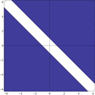
Figure 1: The sets $E=E^{\circ}$ and $E^{\diamond}$.

For example, for a bivariate isometric Cauchy process $Z$ with the jump measure $\nu(dz)=\|z\|^{-3}\,dz$, $z\neq 0$, we obtain $H(\varepsilon^{-1})=2\pi\varepsilon$, $m(E)\approx 0.49$, $m(E^{\diamond})\approx 0.45$ and hence $\mathbf{E}\tau_{x}(\varepsilon)\approx\mathbf{E}\tau_{x}^{\circ}(\varepsilon)\approx 0.33/\varepsilon$, $\mathbf{E}\tau_{x}^{\diamond}(\varepsilon)\approx 0.35/\varepsilon$.

Example 3.2 (Reduction to additive noise for $n=m=1$)

In the case $n=m=1$, the exit time $\tau^{\diamond}$ can be obtained with help of the change of variables formula (2.8) and a trick which was used by Nourdin and Simon in [35]. Consider a one-dimensional canonical Marcus equation

$$X_{t}^{\diamond}=X_{0}-\int_{0}^{t}U^{\prime}(X_{s}^{\diamond})\,ds+\varepsilon\int_{0}^{t}F(X_{s-}^{\diamond})\diamond dZ_{s}$$

driven by a univariate Lévy process $Z$ and let $\mathcal{G}=(-a,b)$, $a,b>0$. Assume that the perturbation is uniformly elliptic in $\mathcal{G}$, that is $F(x)>0$, $x\in[-a,b]$, and introduce the function

$$f(x)=\int_{0}^{x}\frac{dy}{F(y)},\quad f^{\prime}(x)=\frac{1}{F(x)},\quad x\in[-a,b].$$

Applying the change of variables formula (2.8) yields the following SDE for the process $Y^{\diamond}_{t}=f(X_{t}^{\diamond})$:

$$Y^{\diamond}_{t}=f(X_{t}^{\diamond}) =f(x)-\int_{0}^{t}f^{\prime}(X_{s}^{\diamond})U^{\prime}(X_{s}^{\diamond})\,ds+\varepsilon\int_{0}^{t}f^{\prime}(X^{\diamond}_{s-})F(X_{s-}^{\diamond})\diamond dZ_{s}$$

$$=f(x)-\int_{0}^{t}f^{\prime}(X_{s}^{\diamond})U^{\prime}(X_{s}^{\diamond})\,ds+\varepsilon Z_{t}$$

$$=y^{\diamond}+\int_{0}^{t}B^{\diamond}(Y_{s}^{\diamond})\,ds+\varepsilon Z_{t}$$

with $B^{\diamond}(y):=-\frac{U^{\prime}}{F}\circ f^{-1}(y)$ and $y^{\diamond}=f(x)$. Note that since $F$ is strictly positive and $f$ is monotone increasing with $f(0)=0$, we can introduce the new effective potential $U^{\diamond}(y)=-\int_{0}^{y}B^{\diamond}(v)\,dv$ which is a one-well potential with the global minimum at the origin. Thus the process $Y^{\diamond}_{t}$ satisfies the SDE with additive small noise which has been studied in Imkeller and Pavlyukevich [21, 23] and Imkeller et al. [25]. It is clear that $X_{t}^{\diamond}\notin(-a,b)$ if and only if $Y^{\diamond}_{t}\notin(f^{-1}(a),f^{-1}(b))$.

For instance, if $Z$ is a symmetric $\alpha$-stable Lévy process with $\alpha\in(0,2)$ and the jump measure $\nu(dz)=|z|^{-1-\alpha}\,dz$, $z\neq 0$, then for the first exit time of $X^{\diamond}$ from $(-a,b)$ we immediately obtain the asymptotics

$$\lim_{\varepsilon\downarrow 0}\mathbf{E}e^{-uM^{\diamond}\frac{2}{\alpha}\varepsilon^{\alpha}\tau_{x}^{\diamond}}=\frac{1}{1+u},\quad u>-1,$$

with

$$M^{\diamond}=\Big{(}\frac{1}{|f^{-1}(-a)|^{\alpha}}+\frac{1}{|f^{-1}(b)|^{\alpha}}\Big{)}^{-1}.$$

4 First exit time of the Itô SDE with multiplicative noise

4.1 Big and small jumps of $Z$

For $\rho\in(0,1)$ and $\varepsilon\leq 1$ let us distinguish the small and big jumps of the driving process $Z$ and decompose it into a sum

$$Z_{t}=L_{t}+\eta_{t}$$

with

$$\eta_{t}:=\sum_{s\leq t}\Delta Z_{s}\mathbb{I}\{\|\Delta Z_{s}\|\geq\varepsilon^{-\rho}\}$$

being a compound Poisson process with the characteristic exponent

$$\mathbf{E}e^{i\langle\lambda,\eta_{t}\rangle}=\exp\Big{(}t\int_{\|y\|\geq\varepsilon^{-\rho}}(e^{i\langle\lambda,y\rangle}-1)\nu(dy)\Big{)}.$$

The Lévy process $L$ is a process with bounded jumps, $\|\Delta L_{s}\|\leq\varepsilon^{-\rho}$, and thus possesses all moments. Moreover, it is a sum of its continuous component $L^{c}_{t}=W_{t}+\mu t$ being the Brownian motion with drift, and a pure jump part $L^{d}$.

Denote by $0=\tau_{0}<\tau_{1}<\tau_{2}<\dots$ the successive jump times of $\eta$ and by $J_{k}$ the respective jump sizes. The inter-jump times $T_{k}=\tau_{k}-\tau_{k-1}$ are iid exponentially distributed random variables with the mean value

$$\mathbf{E}T_{k}=\frac{1}{\beta_{\varepsilon}}:=\Big{(}\int_{\|y\|\geq\varepsilon^{-\rho}}\nu(dy)\Big{)}^{\!-1}=\frac{1}{H(\varepsilon^{-\rho})}\to\infty,\quad\varepsilon\to 0,$$

and the probability distribution function $\mathbf{P}(T_{k}\leq u)=1-e^{-u\beta_{\varepsilon}}$, $u\geq 0$. The probability law of $J_{k}$ is also known explicitly in terms of the Lévy measure $\nu$:

$$\mathbf{P}(J_{k}\in A)=\beta_{\varepsilon}^{-1}\nu(A\cap\{z:\ \|z\|\geq\varepsilon^{-\rho}\}),\quad A\in\mathcal{B}(\mathbb{R}^{m}).$$ (4.1)

4.2 Perturbations by the process $\varepsilon L$

Lemma 4.1

Let $\rho\in(0,1)$, $\mu_{\varepsilon}:=\mathbf{E}L_{1}$ and $T_{\varepsilon}:=\varepsilon^{-\theta}$ for some $\theta>0$. There exist $\delta_{0}=\delta_{0}(\rho)>0$ and $\theta_{0}=\theta_{0}(\rho)>0$ such that for all $\delta\in(0,\delta_{0})$, $\theta\in(0,\theta_{0})$ there are $p_{0}=p_{0}(\delta)$ and $\varepsilon_{0}=\varepsilon_{0}(\rho,\delta)$ such that the estimates

$$\|\varepsilon L_{T_{\varepsilon}}\|=\varepsilon\|\mu_{\varepsilon}\|T_{\varepsilon}<\varepsilon^{2\delta}\quad\text{and}\quad\mathbf{P}([\varepsilon L]_{T_{\varepsilon}}^{d}\geq\varepsilon^{\delta})\leq\exp(-\varepsilon^{-p})$$

hold for all $p\in(0,p_{0})$ and $0<\varepsilon\leq\varepsilon_{0}$.

Proof: Let us represent the process $L$ as

$$L_{t}=\tilde{L}_{t}+\mu_{\varepsilon}t$$

with $\tilde{L}$ being a zero mean Lévy martingale with bounded jumps.

Step 1. We have the following estimates for the mean value $\mu_{\varepsilon}$:

$$\mu_{\varepsilon}^{i}:=\mathbf{E}L^{i}_{1}=\int_{1<\|z\|\leq\varepsilon^{-\rho}}z_{i}\,\nu(dz),\quad 1\leq i\leq m,$$

$$\|\mu_{\varepsilon}\|^{2}\leq\int_{1<\|z\|\leq\varepsilon^{-\rho}}\|z\|^{2}\,\nu(dz)=-\int_{1}^{\varepsilon^{-\rho}}u^{2}\,dH(u)\leq\varepsilon^{-2\rho}H(1),$$

$$\|\mu_{\varepsilon}\|\leq\sqrt{H(1)}\varepsilon^{-\rho}.$$

Consequently, for any $\rho\in(0,1)$, $\theta_{0}:=(1-\rho)/3$ and $\delta_{0}:=(1-\rho)/4$ we obtain

$$\varepsilon\|\mu_{\varepsilon}\|T_{\varepsilon}<\varepsilon^{2\delta}$$

for all $0<\delta<\delta_{0}$ and $0<\theta<\theta_{0}$ and $\varepsilon$ small enough.

Step 2. The of quadratic variation process $[\varepsilon\tilde{L}]^{d}_{t}$ is a Lévy subordinator

$${}[\varepsilon\tilde{L}]^{d}_{t}=\varepsilon^{2}\sum_{s\leq t}\|\Delta\tilde{L}\|_{s}^{2}=\varepsilon^{2}\int_{0}^{t}\int_{0<\|z\|\leq\varepsilon^{-\rho}}\|z\|^{2}N(dz,ds).$$

Since the jumps of $[\varepsilon\tilde{L}]^{d}$ are bounded, its Laplace transform is well-defined for all $\lambda\in\mathbb{R}$ and equals

$$\mathbf{E}e^{\lambda[\varepsilon\tilde{L}]^{d}_{t}} =\exp\Big{(}t\int_{0<\|z\|\leq\varepsilon^{-\rho}}(e^{\lambda\varepsilon^{2}\|z\|^{2}}-1)\,\nu(dz)\Big{)}$$ (4.2)

$$=\exp\Big{(}-t\int_{0<u\leq\varepsilon^{-\rho}}(e^{\lambda\varepsilon^{2}u^{2}}-1)\,dH(u)\Big{)}.$$

For any $\lambda>0$, the exponential Chebyshev inequality implies that

$$\mathbf{P}([\varepsilon\tilde{L}]^{d}_{T_{\varepsilon}}>\varepsilon^{\delta}) =\mathbf{P}(e^{\lambda[\varepsilon\tilde{L}]^{d}_{T_{\varepsilon}}}>e^{\lambda\varepsilon^{\delta}})\leq e^{-\lambda\varepsilon^{\delta}}\mathbf{E}e^{\lambda[\varepsilon\tilde{L}]^{d}_{T_{\varepsilon}}}$$ (4.3)

$$=\exp\Big{(}-\lambda\varepsilon^{\delta}-T_{\varepsilon}\int_{0<u\leq\varepsilon^{-\rho}}(e^{\lambda\varepsilon^{2}u^{2}}-1)\,dH(u)\Big{)}.$$

For $\lambda=\lambda_{\varepsilon}:=\varepsilon^{-2\delta}$ with $0<\delta<\delta_{0}=(1-\rho)/4$ we have $\max_{0\leq u\leq\varepsilon^{-\rho}}\lambda_{\varepsilon}\varepsilon^{2}u^{2}\leq\lambda_{\varepsilon}\varepsilon^{2(1-\rho)}\downarrow 0$ as $\varepsilon\downarrow 0$. With help of the elementary inequality $e^{x}-1\leq 2x$ for small positive $x$ the second summand appearing in the exponent in r.h.s. of (4.3) can be now estimated as

$$\Big{|}T_{\varepsilon}\int_{0<u\leq\varepsilon^{-\rho}} (e^{\lambda_{\varepsilon}\varepsilon^{2}u^{2}}-1)\,dH(u)\Big{|}\leq\Big{|}2T_{\varepsilon}\lambda_{\varepsilon}\varepsilon^{2}\Big{(}\int_{0<u\leq 1}+\int_{1<u\leq\varepsilon^{-\rho}}\Big{)}u^{2}\,dH(u)\Big{|}$$

$$\leq 2T_{\varepsilon}\lambda_{\varepsilon}\varepsilon^{2}\Big{|}\int_{0<u\leq 1}u^{2}\,dH(u)\Big{|}+2T_{\varepsilon}\lambda_{\varepsilon}\varepsilon^{2(1-\rho)}\Big{|}\int_{1<u\leq\varepsilon^{-\rho}}\,dH(u)\Big{|}$$

$$\leq CT_{\varepsilon}\lambda_{\varepsilon}\varepsilon^{2}+2H(1)T_{\varepsilon}\lambda_{\varepsilon}\varepsilon^{2(1-\rho)}$$

with $C=\big{|}\int_{0<u\leq 1}u^{2}\,dH(u)\big{|}>0$. Consequently, for all $0<\delta<\delta_{0}$ and $0<\theta<\theta_{0}$ we see that the exponential inequality

$$\mathbf{P}([\varepsilon\tilde{L}]^{d}_{T_{\varepsilon}}>\varepsilon^{\delta}) \leq\exp\Big{(}-\lambda_{\varepsilon}\varepsilon^{\delta}+CT_{\varepsilon}\lambda_{\varepsilon}\varepsilon^{2}+2H(1)T_{\varepsilon}\lambda_{\varepsilon}\varepsilon^{2(1-\rho)}\Big{)}\leq e^{-\varepsilon^{-\delta/2}}$$

holds for $\varepsilon$ small enough and the Lemma holds with $p\in(0,\delta/2)$. $\blacksquare$

Lemma 4.2

Let $\rho\in(0,1)$ and $(g_{t})_{t\geq 0}$ be a bounded adapted càdlàg stochastic process mit values in $\mathbb{R}^{m}$, $T_{\varepsilon}=\varepsilon^{-\theta}$, $\theta>0$. There are $\delta_{0}=\delta_{0}(\rho)>0$ and $\theta_{0}=\theta_{0}(\rho)>0$ such that for all $\delta\in(0,\delta_{0})$ and $\theta\in(0,\theta_{0})$ there are $p_{0}=p_{0}(\rho,\delta)$ and $\varepsilon_{0}=\varepsilon_{0}(\delta)$ such that the exponential estimate

$$\mathbf{P}\Big{(}\sup_{0\leq t\leq T_{\varepsilon}}\varepsilon\Big{|}\sum_{j=1}^{m}\int_{0}^{t}g^{j}_{s-}\,d\tilde{L}^{j}_{s}\Big{|}\geq\varepsilon^{\delta}\Big{)}\leq e^{-\varepsilon^{-p}}.$$

holds for all $p\in(0,p_{0})$ and $0<\varepsilon\leq\varepsilon_{0}$.

Proof: Step 1. Suppose that $\sup_{t\geq 0}\|g_{t}\|\leq C$ for some $C>0$. Consider the one-dimensional martingale

$$M_{t}=\sum_{j=1}^{m}\int_{0}^{t}g^{j}_{s-}\,d\tilde{L}^{j}_{s}.$$

By construction $|\Delta M_{t}|\leq C\varepsilon^{-\rho}$. We estimate the probability of a deviation of the size $\varepsilon^{\delta}$ of $\varepsilon M_{t}$ from zero with help of the exponential inequality for martingales, see Theorem 26.17(i) in Kallenberg [26]. Indeed for any $\delta>0$ and $\theta>0$ we have

$$\mathbf{P}\Big{(}\sup_{t\leq T_{\varepsilon}}|\varepsilon M_{t}|\geq\varepsilon^{\delta}\Big{)}\leq\mathbf{P}\Big{(}\sup_{t\leq T_{\varepsilon}}|\varepsilon M_{t}|\geq\varepsilon^{\delta}\Big{|}[\varepsilon M]_{T_{\varepsilon}}\leq\varepsilon^{4\delta}\Big{)}+\mathbf{P}([\varepsilon M]_{T_{\varepsilon}}>\varepsilon^{4\delta}).$$

Inspecting the proofs of Lemma 26.19 and Theorem 26.17(i) in Kallenberg [26] we get that for any $\lambda>0$

$$\mathbf{P}\Big{(}\sup_{t\leq T_{\varepsilon}}\varepsilon M_{t}\geq\varepsilon^{\delta}\Big{|}[\varepsilon M]_{T_{\varepsilon}}\leq\varepsilon^{4\delta}\Big{)}\leq e^{-\lambda\varepsilon^{\delta}+\lambda^{2}h(\lambda C\varepsilon^{1-\rho})\varepsilon^{4\delta}}$$

with $h(x)=-(x+\ln(1-x)_{+})x^{-2}$. For any $0<\delta<\delta_{1}:=(1-\rho)/2$ we set $\lambda=\lambda_{\varepsilon}=\varepsilon^{-2\delta}$, so that $h(\lambda_{\varepsilon}C\varepsilon^{1-\rho})\to 1/2$ as $\varepsilon\to 0$. Hence we obtain the estimate

$$\mathbf{P}\Big{(}\sup_{t\leq T_{\varepsilon}}\varepsilon M_{t}\geq\varepsilon^{\delta}\Big{|}[\varepsilon M]_{T_{\varepsilon}}\leq\varepsilon^{4\delta}\Big{)}\leq e^{-\varepsilon^{-\delta/2}}\leq e^{-\varepsilon^{-p}},$$

which holds for $\varepsilon$ small enough and $p\in(0,\delta/2)$. An analogous inequality holds for $\inf_{t\leq T_{\varepsilon}}\varepsilon M_{t}$.

Step 2. There is a constant $C_{1}>0$ with

$${}[\varepsilon M]_{t}=\int_{0}^{t}g_{s}^{2}\,d[\varepsilon W]_{s}+\int_{0}^{t}g_{s-}^{2}\,d[\varepsilon\tilde{L}]^{d}_{s}\leq C_{1}(\varepsilon^{2}t+[\varepsilon\tilde{L}]^{d}_{t}),\quad t\geq 0.$$

For sufficiently small $\varepsilon$ we obtain the estimate

$$\mathbf{P}([\varepsilon M]_{T_{\varepsilon}}\geq\varepsilon^{4\delta})\leq\mathbf{P}([\varepsilon\tilde{L}]^{d}_{T_{\varepsilon}}\geq\varepsilon^{5\delta})+\mathbf{P}(C_{1}\varepsilon^{2}T_{\varepsilon}\geq\varepsilon^{5\delta}).$$

For $\varepsilon$ small enough the second summand vanishes for all $0<\delta<\delta_{2}$, $0<\theta<\theta_{2}$ with $0<\theta_{2}+5\delta_{2}<2$. The first summand is bounded by $e^{-\varepsilon^{-p}}$ from above due to Lemma 4.1 for $0<\delta<\delta_{3}$ some $0<\theta<\theta_{3}$ and $0<p<p_{1}(\rho,\delta)$ and $\varepsilon$ small enough. This the statement of the Lemma holds with $\delta_{0}=\min\{\delta_{1},\delta_{2},\delta_{3}\}$, $\theta_{0}=\min\{\theta_{1},\theta_{2},\theta_{3}\}$ and $p_{0}=\min\{\delta/2,p_{1}(\delta)\}$. $\blacksquare$

Lemma 4.3

For any $\rho\in(0,1)$ there are $\gamma_{0}>0$ and $p>0$ such that for all $0<\gamma\leq\gamma_{0}$

$$\sup_{x\in\mathcal{G}}\mathbf{P}\Big{(}\sup_{0\leq t<T_{1}}\|X(t,x)-Y(t,x)\|\geq\varepsilon^{\gamma}\Big{)}\leq e^{-\varepsilon^{-p}}.$$

Proof: Step 1. By assumptions on the potential $U$, any deterministic trajectory $Y_{t}(y)$, $y\in\mathcal{G}$, reaches a small fixed neighbourhood of the origin in some finite time. After entering this small neighbourhood, the trajectory $Y_{t}(y)$ is attracted to the origin with the speed approximately proportional to $C_{1}\|Y_{t}\|$, $C_{1}>0$ being the smallest eigenvalue of the matrix $\frac{\partial^{2}}{\partial x_{i}\partial x_{j}}U(x)\big{|}_{x=0}$. This allows us to estimate of increase rate of the time a trajectory $Y_{t}(y)$, $y\in\mathcal{G}$, needs to reach some $\varepsilon^{\delta}$-neighbourhood of the origin. Indeed, for any $\delta>0$ the following inequality holds true for any $0\leq\varepsilon\leq\varepsilon_{0}$, $y\in\mathcal{G}$ and $\varepsilon_{0}>0$ small enough:

$$\|Y_{t}(y)\|\leq\varepsilon^{\delta},\quad t\geq V_{\varepsilon}:=\frac{2\delta}{C_{1}}|\ln\varepsilon|.$$ (4.4)

Step 2. Here we show that on the time intervals up to $V_{\varepsilon}$, the random trajectory $X^{\varepsilon}(x)$ does not deviate much from the deterministic solution $Y_{t}(x)$ with the same initial value in the absence of big jumps of the driving process $Z$.

For $x\in\mathcal{G}$, with help of Gronwall’s lemma we estimate

$$\|X_{t\wedge V_{\varepsilon}\wedge T_{1}-}-Y_{t\wedge V_{\varepsilon}\wedge T_{1}-}\|$$

$$\qquad\qquad\leq C_{\text{Lip}}\int_{0}^{t\wedge V_{\varepsilon}\wedge T_{1}-}\|X_{s}-Y_{s}\|\,ds+\varepsilon\Big{\|}\int_{0}^{t\wedge V_{\varepsilon}\wedge T_{1}-}F(X_{s-})\,dZ_{s}\Big{\|},$$

$$\sup_{0\leq t<V_{\varepsilon}\wedge T_{1}}\|X_{t}-Y_{t}\|\leq e^{C_{\text{Lip}}V_{\varepsilon}}\sup_{0\leq t\leq V_{\varepsilon}}\varepsilon\Big{\|}\int_{0}^{t}F(X_{s-})\,dL_{s}\Big{\|}.$$

Recalling the definition of $V_{\varepsilon}$ in (4.4) and taking into account that $V_{\varepsilon}\leq T_{\varepsilon}=\varepsilon^{-\theta}$ for $\varepsilon$ small enough and any $\theta>0$ we get for any $\delta>0$ that

$$\mathbf{P}\Big{(}\sup_{0\leq t<V_{\varepsilon}\wedge T_{1}} \|X_{t}-Y_{t}\|\geq\varepsilon^{\delta}\Big{)}\leq\mathbf{P}\Big{(}\sup_{0\leq t\leq V_{\varepsilon}}\varepsilon\Big{\|}\int_{0}^{t}F(X_{s-})\,dL_{s}\Big{\|}\geq\varepsilon^{(1+\frac{2C_{\text{Lip}}}{C_{1}})\delta}\Big{)}$$

$$\leq\mathbf{P}\Big{(}\sup_{0\leq t\leq T_{\varepsilon}}\varepsilon\Big{\|}\int_{0}^{t}F(X_{s-})\,d\tilde{L}_{s}\Big{\|}+C_{2}\varepsilon T_{\varepsilon}\|\mu_{\varepsilon}\|\geq\varepsilon^{(1+\frac{2C_{\text{Lip}}}{C_{1}})\delta}\Big{)}$$

with some $C_{2}>0$. With help of Lemmas 4.1 and 4.2 we find that there are $\delta_{1}>0$ and $\theta_{1}>0$ such that the last probability is smaller than $\exp(-\varepsilon^{-p})$ for all $\delta\in(0,\delta_{1})$, $\theta\in(0,\theta_{1})$ and $p\in(0,p_{1}(\delta))$.

Step 3. In this Step we exploit the attractor property of the origin and show that in the absence of big jumps of the driving process $Z$ the random path $X_{t}(x)$ with the initial value close to the origin does not deviate much on the polynomially long time intervals $T_{\varepsilon}$.

Consider the function $f(x)=\ln(1+U(x))\geq 0$. For $\|x\|$ small, one can estimate $c_{1}\|x\|^{2}\leq f(x)\leq c_{2}\|x\|^{2}$ for some positive $c_{1}$ and $c_{2}$. Furthermore, the derivatives $\partial_{i}f(x)=\frac{\partial_{i}U(x)}{1+U(x)}$, $\partial_{i}\partial_{j}f(x)=2\frac{\partial_{i}U(x)\partial_{j}U(x)-\partial_{i}\partial_{j}U(x)}{(1+U(x))^{2}}$ are bounded due to assumptions on $U$.

We apply the Itô formula to the process $f(X_{t})$:

$$0 \leq f(X_{t\wedge T_{\varepsilon}\wedge T_{1}-})$$

$$\begin{aligned} =f(x)&+\sum_{i=1}^{n}\int_{0}^{t\wedge T_{\varepsilon}\wedge T_{1}-}\!\!\partial_{i}f(X_{s-})\,dX^{i}_{s}+\frac{1}{2}\sum_{i,j=1}^{n}\int_{0}^{t\wedge T_{\varepsilon}\wedge T_{1}-}\!\!\partial_{i}\partial_{j}f(X_{s-})\,d[X^{i},X^{j}]^{c}_{s}\\ &+\sum_{s<{t\wedge T_{\varepsilon}\wedge T_{1}}}\Big{(}f(X_{s})-f(X_{s-})-\sum_{i=1}^{n}\partial_{i}f(X_{s-})\Delta X^{i}_{s}\Big{)}\\ =f(x)&-\int_{0}^{t\wedge T_{\varepsilon}\wedge T_{1}-}\!\frac{\|\nabla U(X_{s-})\|^{2}}{1+U(X_{s-})}\,ds+\varepsilon\sum_{i,j=1}^{n,m}\!\int_{0}^{t\wedge T_{\varepsilon}\wedge T_{1}-}\frac{\partial_{i}U(X_{s-})F_{ij}(X_{s-})}{1+U(X_{s-})}\,dZ^{j}_{s}\\ &+\frac{\varepsilon^{2}}{2}\sum_{i,j=1}^{n}\sum_{k,l=1}^{m}\int_{0}^{t\wedge T_{\varepsilon}\wedge T_{1}-}\partial_{i}\partial_{j}f(X_{s-})F_{ik}(X_{s-})F_{jl}(X_{s-})\,d[Z^{k},Z^{l}]^{c}_{s}\\ &+\sum_{s<{t\wedge T_{\varepsilon}\wedge T_{1}}}\Big{(}f(X_{s})-f(X_{s-})-\sum_{i=1}^{n}\partial_{i}f(X_{s-})\Delta X^{i}_{s}\Big{)}.\end{aligned}$$

We note that the first integral in the last formula is non-negative, the integrands in the Itô integral w.r.t. $Z$ and in the integrals w.r.t. $[Z^{k},Z^{l}]^{c}$ are bounded, the quadratic covariations satisfy $[Z^{k},Z^{l}]^{c}_{t}=[W^{k},W^{l}]_{t}=\sigma_{kl}t$, and finally the estimate

$$\sum_{s\leq t}\Big{|}f(X_{s}) -f(X_{s-})-\sum_{i=1}^{n}\partial_{i}f(X_{s-})\Delta X^{i}_{s}\Big{|}$$

$$\leq\frac{1}{2}\sum_{i,j=1}^{n}\sum_{s\leq t}\Big{|}\int_{0}^{1}(1-v)\partial_{i}\partial_{j}f(X_{s-}+v\Delta X_{s})\,dv\Big{|}\cdot|\Delta X^{i}_{s}\Delta X^{j}_{s}|$$

$$\leq C_{3}\sum_{s\leq t}\|\Delta X_{s}\|^{2}=C_{3}[X]_{t}^{d}$$

holds with some $C_{3}>0$. Furthermore, since $F$ is bounded the estimate

$${}[X]_{t}^{d}\leq C_{4}[Z]^{d}_{t}=C_{4}[L]^{d}_{t}$$

holds for some constant $C_{4}>0$ and $0\leq t<T_{1}$. Combining these estimates and denoting $g(x)=\frac{\nabla^{T}U(x)F(x)}{1+U(x)}$ we obtain the following estimate with some positive constant $C_{5}$, $\varepsilon$ small enough and $\|x\|\leq\varepsilon^{\delta}$, $\delta>0$:

$$0\leq f(X_{t\wedge T_{\varepsilon}\wedge T_{1}-})\leq C_{5}\Big{(}\varepsilon^{2\delta}+\varepsilon\sup_{0\leq t\leq T_{\varepsilon}}\Big{|}\int_{0}^{t}g(X_{s-})\,d\tilde{L}_{s}\Big{|}+\varepsilon\|\mu_{\varepsilon}\|T_{\varepsilon}+\varepsilon^{2}{T_{\varepsilon}}+\varepsilon^{2}[L]^{d}_{T_{\varepsilon}}\Big{)}.$$

Let the estimates of the Lemmas 4.1 and 4.2 hold simultaneously for $\delta\in(0,\delta_{2})$, $\theta\in(0,\theta_{2})$ and $p\in(0,p_{2}(\delta))$ for some positive $\delta_{2}$, $\theta_{2}$, $p_{2}(\delta)$ and $\varepsilon$ small. Then for $\delta\in(0,\delta_{2}/3)$, $\theta\in(0,\theta_{1})$ and $\varepsilon$ small we get

$$\mathbf{P}\Big{(}\sup_{0\leq t<T_{\varepsilon}\wedge T_{1}} \|X_{t}\|\geq\varepsilon^{\delta}\Big{)}\leq\mathbf{P}\Big{(}\varepsilon^{2\delta}\geq\varepsilon^{3\delta}\Big{)}+\mathbf{P}\Big{(}\varepsilon\sup_{0\leq t\leq T_{\varepsilon}}\Big{|}\int_{0}^{t}g(X_{s-})\,d\tilde{L}_{s}\Big{|}\geq\varepsilon^{3\delta}\Big{)}$$

$$+\mathbf{P}\Big{(}\varepsilon\|\mu_{\varepsilon}\|T_{\varepsilon}\geq\varepsilon^{3\delta}\Big{)}+\mathbf{P}\Big{(}\varepsilon^{2}{T_{\varepsilon}}\geq\varepsilon^{3\delta}\Big{)}+\mathbf{P}\Big{(}\varepsilon^{2}[L]^{d}_{T_{\varepsilon}}\geq\varepsilon^{3\delta}\Big{)}\leq e^{-\varepsilon^{-p}}.$$

for $p\in(0,p_{2}(\delta)/2)$.

Step 4. Combining the estimates of Steps 1, 2 and 3, we extend the estimate of the Step 3 to all initial values $x\in\mathcal{G}$:

$$\mathbf{P}\Big{(}\sup_{0\leq t<T_{\varepsilon}\wedge T_{1}}\|X_{t}-Y_{t}\|\geq\varepsilon^{\delta}\Big{)}\leq e^{-\varepsilon^{-p}}$$

for $\delta\in(0,\delta_{3})$, $\theta\in(0,\theta_{3})$, $p\in(0,p_{3}(\delta))$ and $\varepsilon$ small enough. Here, $\delta_{3}=\min\{\delta_{1},\delta_{2}/3\}$, $\theta_{3}=\min\{\theta_{1},\theta_{2}\}$ and $p_{3}=\min\{p_{1}(\delta),p_{2}(\delta)/2\}$.

Step 5. In this final Step we extend the estimate of the Step 4 from the time interval $[0,T_{\varepsilon}\wedge T_{1})$ to the time interval $[0,T_{1})$.

Denote $X^{L}$ the solution of the SDE (2.1) driven by the process $L$. Clearly, $X_{t}=X_{t}^{L}$ on the event $\{t<T_{1}\}$. Let $x\in\mathcal{G}$ and $k\geq 1$, then for any $\delta>0$ and $\theta>0$ we have

$$\mathbf{P}\Big{(}\sup_{t\in[0,T_{1})}\|X_{t}-Y_{t}\|\geq\varepsilon^{\delta}\Big{)} \leq\mathbf{P}\Big{(}\sup_{t\in[0,kT_{\varepsilon}\wedge T_{1})}\|X_{t}-Y_{t}\|\geq\varepsilon^{\delta}\Big{)}+\mathbf{P}(T_{1}\geq kT_{\varepsilon})$$

$$\leq\mathbf{P}\Big{(}\sup_{t\in[0,kT_{\varepsilon}]}\|X_{t}^{L}-Y_{t}\|\geq\varepsilon^{\delta}\Big{)}+\mathbf{P}(T_{1}\geq kT_{\varepsilon}).$$

Moreover for $\varepsilon$ small enough we have $\|Y(T_{\varepsilon},x)\|<\varepsilon^{2\delta}$ for $x\in\mathcal{G}$. Denote

$$A_{j}=\{\sup_{t\in[jT_{\varepsilon},(j+1)T_{\varepsilon}]}\|X_{t}^{L}-Y(t-jT_{\varepsilon};X_{jT_{\varepsilon}}^{L})\|<\varepsilon^{\delta}\},\quad 0\leq j\leq k-1.$$

In particular, the probability of $A_{0}^{c}=\{\sup_{t\in[0,T_{\varepsilon}]}\|X_{t}^{L}-Y_{t}\|\geq\varepsilon^{\delta}\}$ was estimated in Step 4. Further, for any $k\geq 1$

$$\bigcap_{j=0}^{k-1}A_{j}\subseteq\Big{\{}\sup_{t\in[0,kT_{\varepsilon}]}\|X_{t}^{L}-Y_{t}\|<2\varepsilon^{\delta}\Big{\}}.$$

Consequently

$$\mathbf{P}\Big{(}\sup_{t\in[0,kT_{\varepsilon}]}\|X^{L}_{t}-Y_{t}\| \geq 2\varepsilon^{\delta}\Big{)}\leq\mathbf{P}\Big{(}\bigcup_{j=0}^{k-1}A_{j}^{c}\Big{)}$$ (4.5)

$$=\mathbf{P}\Big{(}A_{0}^{c}\cup(A_{0}A_{1}^{c})\cup\cdots\cup(A_{0}\cdots A_{k-2}A_{k-1}^{c})\Big{)}$$

$$\leq\sum_{j=0}^{k-1}\mathbf{P}(A_{j}^{c},\|X^{L}_{jT_{\varepsilon}}\|\in\mathcal{G})\leq k\sup_{x\in\mathcal{G}}\mathbf{P}(A_{0}^{c}).$$

For $k=k_{\varepsilon}=[\varepsilon^{-2r}]$ and any $\theta>0$ we have

$$\mathbf{P}(T_{1}\geq k_{\varepsilon}T_{\varepsilon})=e^{-k_{\varepsilon}T_{\varepsilon}\beta_{\varepsilon}}\leq\exp(-\varepsilon^{r\rho-\theta-2r}l(\varepsilon^{-\rho}))\leq e^{-\varepsilon^{-p}}.$$

for all $0<p<p_{4}:=(2-\rho)r$ and $\varepsilon$ small. On the other hand, (4.5) and Step 4 yield

$$\mathbf{P}(\sup_{t\in[0,kT_{\varepsilon}]}\|X^{L}_{t}-Y_{t}\|\geq 2\varepsilon^{\delta})\leq\varepsilon^{-2r}e^{-\varepsilon^{-p}}\leq e^{-\varepsilon^{-p/2}}$$

with any $0<p<p_{3}(\delta)$. Consequently, the statement of the Lemma holds for any $0<\gamma<\delta_{3}$, $0<p<\min\{p_{3}(\gamma)/2,p_{4}\}$ and $\varepsilon$ small enough. $\blacksquare$

4.3 The first exit time of solutions of the Itô SDE

Having established the key estimates about deviations of the random trajectory $X_{t}(x)$ from the deterministic path $Y_{t}(x)$ on random time intervals between big jumps of the driving process $Z$ we can calculate the asymptotics of the Laplace transform of the first exit time. The proof here goes along the lines of the one-dimensional case considered in Imkeller and Pavlyukevich [22] and the multivariate case of a dynamical system driven by a multifractal $\alpha$-stable noise considered in Imkeller et al. [24]. For the sake of completeness we briefly sketch the main idea of the proof.

The argument is based on the concept of the one big jump which is often used in the study of heavy tail phenomena. Roughly speaking, it can be shown that under certain conditions the small perturbations of the dynamical system $Y$ due the process $\varepsilon L$ can be neglected, and the exit from the domain occurs with high probability at one of the jump times $\tau_{k}$. Just before the time $\tau_{k}$ the solution $X$ stays in a small neighbourhood of the stable point, so the exit occurs if the jump $\varepsilon J_{k}$ is large enough, namely if $F(X_{\tau_{k}-})\varepsilon J_{k}\approx F(0)\varepsilon J_{k}\notin\mathcal{G}$. The events $\{\varepsilon J_{1}\notin E\}=\{F(0)\varepsilon J_{1}\in\mathcal{G}\}$,…, $\{\varepsilon J_{k-1}\notin E\}=\{F(0)\varepsilon J_{k-1}\in\mathcal{G}\}$ and $\{\varepsilon J_{k}\in E\}=\{F(0)\varepsilon J_{k}\notin\mathcal{G}\}$ are independent and build up a geometric sequence of events. Their probabilities can be calculated in the limit of $\varepsilon\to 0$ with help of the scaling property of the jump measure $\nu$.

The statement of the main theorem follows from the small noise estimates from below and above of the Laplace transforms of the normalised first exit times. Here we consider the less complicated estimate form below.

For any $u>-1$, with help of the formula of the total probability we have

$$\mathbf{E}e^{-um(E)H(\varepsilon^{-1})\sigma_{x}(\varepsilon)}\geq\sum_{k=1}^{\infty}\mathbf{E}\Big{[}e^{-um(E)H(\varepsilon^{-1})\tau_{k}}\mathbb{I}\{\sigma=\tau_{k}\}\Big{]}.$$ (4.6)

For any $\delta>0$ small enough denote $\mathcal{G}^{-\delta}:=\{x\in\mathcal{G}:\ \operatorname{dist}(\partial G,x)\geq\delta\}$ the inner part of $\mathcal{G}$ and $\mathcal{G}^{+\delta}\equiv\mathcal{G}^{\delta}:=\{x\in\mathbb{R}^{n}:\ \operatorname{dist}(G,x)\leq\delta\}$ be the outer $\delta$-neighbourhood. For $k\geq 1$, the strong Markov property allows to write

$$\mathbf{E} \Big{[}e^{-um(E)H(\varepsilon^{-1})\tau_{k}}\mathbb{I}\{\sigma=\tau_{k}\}\Big{]}$$ (4.7)

$$=\mathbf{E}\Big{[}e^{-um(E)H(\varepsilon^{-1})\tau_{k}}\mathbb{I}\{X_{t}\in\mathcal{G},t\in[0,\tau_{k}),X_{\tau_{k}}\notin\mathcal{G}\}\Big{]}$$

$$=\mathbf{E}\Big{[}\prod_{j=1}^{k-1}e^{-um(E)H(\varepsilon^{-1})T_{j}}\mathbb{I}\{X_{t+\tau_{j-1}}\in\mathcal{G},t\in[0,T_{j}]\}$$

$$\qquad\quad\times e^{-um(E)H(\varepsilon^{-1})T_{k}}\mathbb{I}\{X_{t+\tau_{k-1}}\in\mathcal{G},t\in[0,T_{k})\}\mathbb{I}\{X_{\tau_{k}}\notin\mathcal{G}\}\Big{]}$$

$$\geq\Big{(}\inf_{y\in\mathcal{G}^{-\delta}}\mathbf{E}\Big{[}e^{-um(E)H(\varepsilon^{-1})T_{1}}\mathbb{I}\{X_{t}(y)\in\mathcal{G}^{-\delta},t\in[0,T_{1}]\}\Big{]}\Big{)}^{k-1}$$

$$\qquad\quad\times\inf_{y\in\mathcal{G}^{-\delta}}\mathbf{E}\Big{[}e^{-um(E)H(\varepsilon^{-1})T_{1}}\mathbb{I}\{X_{t}(y)\in\mathcal{G},t\in[0,T_{1})\}\mathbb{I}\{X_{T_{1}}\notin\mathcal{G}\}\Big{]}.$$

Let $\gamma>0$ be such that the estimates of the Section 4.2 hold. We set $\delta:=\delta(\varepsilon)=\varepsilon^{\gamma}$. The exit from the domain with a big jump $\varepsilon J_{1}$ occurs when $F(X_{T_{1}-})\varepsilon J_{1}\notin\mathcal{G}$. Further, $\sup_{0\leq t<T_{1}}\|X_{t}-Y_{t}\|\leq\frac{1}{2}\varepsilon^{\gamma}$ with probability exponentially close to 1 (Lemma 4.3), $Y_{t}(x)$ reaches a $\frac{1}{2}\varepsilon^{\gamma}$-neighbourhood of the origin during the relaxation time $V_{\varepsilon}=\mathcal{O}(|\ln\varepsilon|)$, and $T_{1}>V_{\varepsilon}$ with high probability. Taking into account that $T_{1}$ is exponentially distributed with the parameter $\beta_{\varepsilon}$ we calculate the Laplace transform of $m(E)H(\varepsilon^{-1})T_{1}$ explicitly, namely

$$\mathbf{E}e^{-um(E)H(\varepsilon^{-1})T_{1}}=\frac{\beta_{\varepsilon}}{\beta_{\varepsilon}+um(E)H(\varepsilon^{-1})}=\frac{1}{1+ua_{\varepsilon}},\quad a_{\varepsilon}:=m(E)\frac{H(\varepsilon^{-1})}{H(\varepsilon^{-\rho})}.$$

Recalling the probability law of big jumps (4.1) we see that for $\varepsilon$ small enough

$$\mathbf{P}(F(0)\varepsilon J_{k}\notin\mathcal{G})=\mathbf{P}(\varepsilon J_{k}\in E)=\frac{\nu(E/\varepsilon)}{\beta_{\varepsilon}}$$ (4.8)

whereas for any $\delta^{\prime}>0$

$$a_{\varepsilon}(1-\delta^{\prime})\leq\frac{\nu(E/\varepsilon)}{\beta_{\varepsilon}}\leq a_{\varepsilon}(1+\delta^{\prime}).$$ (4.9)

To obtain the final asymptotics we have to estimate carefully the perturbed the exit probabilities $\mathbf{P}(F(y)\varepsilon J_{1}\in\mathcal{G}^{-\varepsilon^{\gamma}})$ and $\mathbf{P}(F(y)\varepsilon J_{1}\notin\mathcal{G})$ uniformly over $\|y\|\leq\varepsilon^{\gamma}$. This is achieved with help of the continuity of the function $(y,z)\mapsto F(y)z$ both in $y$ and $z$. Indeed, for any $\delta^{\prime}>0$ we can choose $R>0$ big enough, such that the estimate

$$\mathbf{P}(\|\varepsilon J_{k}\|>R)\leq\frac{\delta^{\prime}}{4}\frac{H(\varepsilon^{-1})}{H(\varepsilon^{-\rho})}$$

holds for $\varepsilon$ small. Further, the function $F(y)z$ is uniformly continuous in $z$ in the ball $\|z\|\leq R$ and is continuous in $y$ at the origin. Using the scaling property of the jump measure $\nu$ and the fact that the limiting measure $m$ has no atoms we show that uniformly over $\|y\|\leq\varepsilon^{\gamma}$

$$|\mathbf{P}(F(y)\varepsilon J_{k}\notin\mathcal{G}^{\pm\varepsilon^{\gamma}},\|\varepsilon J_{k}\|\leq R)-\mathbf{P}(F(0)\varepsilon J_{k}\notin\mathcal{G},\|\varepsilon J_{k}\|\leq R)|\leq\frac{\delta^{\prime}}{4}\frac{H(\varepsilon^{-1})}{H(\varepsilon^{-\rho})},$$

and

$$\mathbf{P}(F(0)\varepsilon J_{k}\notin\mathcal{G})-\mathbf{P}(F(0)\varepsilon J_{k}\notin\mathcal{G},\|\varepsilon J_{k}\|\leq R)\leq\frac{\delta^{\prime}}{4}\frac{H(\varepsilon^{-1})}{H(\varepsilon^{-\rho})}.$$

Finally for any $\delta>0$ we choose $\delta^{\prime}>0$ small enough to get the uniform estimates

$$\inf_{\|y\|\leq\varepsilon^{-\gamma}}\mathbf{P}(F(y)\varepsilon J_{1}\in\mathcal{G}^{-\varepsilon^{\gamma}})\geq 1-m(E)\frac{H(\varepsilon^{-1})}{H(\varepsilon^{-\rho})}(1+\delta)=1-a_{\varepsilon}(1+\delta),$$

$$\inf_{\|y\|\leq\varepsilon^{-\gamma}}\mathbf{P}(F(y)\varepsilon J_{1}\notin\mathcal{G})\geq m(E)\frac{H(\varepsilon^{-1})}{H(\varepsilon^{-\rho})}(1-\delta)=a_{\varepsilon}(1-\delta).$$

for $\varepsilon$ small enough.

Following the lines of the proof of [22] and [24], for any $\delta>0$ and $\varepsilon$ small we can also obtain the multiplicative estimates for the Laplace transforms for any $u>-1$:

$$\inf_{y\in\mathcal{G}^{-\varepsilon^{\gamma}}}\mathbf{E}\Big{[}e^{-um(E)H(\varepsilon^{-1})T_{1}}\mathbb{I}\{X_{t}(y)\in\mathcal{G}^{-\varepsilon^{\gamma}},t\in[0,T_{1}]\}\Big{]}\geq\frac{1-a_{\varepsilon}(1+\delta)}{1+ua_{\varepsilon}},$$

$$\inf_{y\in\mathcal{G}^{-\varepsilon^{\gamma}}}\mathbf{E}\Big{[}e^{-um(E)H(\varepsilon^{-1})T_{1}}\mathbb{I}\{X_{t}(y)\in\mathcal{G}^{-\varepsilon^{\gamma}},t\in[0,T_{1})\}\mathbb{I}\{X_{T_{1}}\notin\mathcal{G}\}\Big{]}\geq\frac{a_{\varepsilon}(1-\delta)}{1+ua_{\varepsilon}}.$$

Summing up the terms from (4.7) over $k\geq 1$ yields the estimate

$$\mathbf{E}e^{-um(E)H(\varepsilon^{-1})\sigma_{x}(\varepsilon)} \geq\frac{a_{\varepsilon}(1-\delta)}{1+ua_{\varepsilon}}\sum_{k=1}^{\infty}\Big{(}\frac{1-a_{\varepsilon}(1+\delta)}{1+ua_{\varepsilon}}\Big{)}^{k-1}$$

$$=\frac{1-\delta}{1+u+\delta}\geq\frac{1}{1+u}-C(u)\delta$$

for some $C(u)>0$ and $\varepsilon$ small.

The upper bound for the Laplace transform is technically more involved since it additionally demands careful estimates of the probability to exit from the domain due to small jumps during the inter-jump intervals of the compound Poisson process $\eta$. These estimates are obtained analogously to the one-dimensional and multi-dimensional cases studied in [22, 24] and finally lead to the uniform convergence of the Laplace transform over $x\in\mathcal{G}^{-\varepsilon^{\gamma}}$ as $\varepsilon\to 0$.

5 First exit time of the Stratonovich SDE

Recalling the Itô form of the Stratonovich SDE (2.3), we reduce the exit problem of $X^{\circ}$ to the Itô case. Indeed, in the argument of the Section 4.3 we have to take into account the Stratonovich correction term $\frac{\varepsilon^{2}}{2}\int_{0}^{t}F^{\prime}(X_{s}^{\circ})F(X_{s}^{\circ})d[Z,Z]^{c}$ which is a Lebesgue integral whose absolute value increases at most as $C\varepsilon^{2}t$ for some $C>0$. It is clear that adding this term to the equation does not influence the estimates of the section 4.2. Thus the result follows immediately, and we obtain the same asymptotics of the first exit time as in the Itô case.

6 First exit time of the Marcus (canonical) SDE

The analysis of the canonical Marcus SDE can also be reduced to the Itô case. As in Section 4.3 above let us distinguish between big and small jumps of $Z$. Since the processes $\eta$ and $L=Z-\eta$ are independent, the Marcus equation can be rewritten in the Itô form as

$$X^{\diamond}_{t}=x -\int_{0}^{t}\nabla U(X^{\diamond}_{s})\,ds+\varepsilon\int_{0}^{t}F(X^{\diamond}_{s-})\circ dZ^{c}_{s}+\varepsilon\int_{0}^{t}F(X^{\diamond}_{s-})\,dL^{d}_{s}$$

$$+\sum_{s\leq t}\Big{(}\varphi^{\varepsilon\Delta L^{d}_{s}}(X^{\diamond}_{s-})-X^{\diamond}_{s-}+F(X^{\diamond}_{s-})\varepsilon\Delta L^{d}_{s}\Big{)}+\sum_{s\leq t}\Big{(}\varphi^{\varepsilon\Delta\eta_{s}}(X^{\diamond}_{s-})-X^{\diamond}_{s-}\Big{)}.$$

Let us estimate the small jump correction term in the Marcus equation. The jumps of the process $\varepsilon L^{d}$ are bounded in absolute value by $\varepsilon^{1-\rho}$. The mapping $u\mapsto\varphi_{u}^{z}$ is $C^{2}(\mathbb{R},\mathbb{R}^{n})$, so the Talyor expansion yields

$$\varphi^{z}(x)=y(1,x;z) =y(0,x;z)+\frac{d}{du}y(0,x;z)+\frac{1}{2}\frac{d^{2}}{du^{2}}y(\theta,x;z)$$

$$=x+F(x)z+R(x,z),\quad\theta\in(0,1),$$

where

$$|R^{k}(x,z)|\leq\frac{1}{2}\sup_{y\in\mathbb{R}^{n}}\Big{|}\sum_{i,j=1}^{m}z_{i}z_{j}\sum_{l=1}^{n}\frac{\partial F_{kj}(y)}{\partial x_{l}}F_{li}(y)\Big{|},\quad 1\leq k\leq n.$$

Since all $F_{li}$ are bounded with bounded derivatives, we obtain the estimate

$$|\varphi^{z}(x)-x-F(x)z|\leq C\|z\|^{2}$$

with some absolute constant $C>0$. This leads to the inequality

$$\Big{|}\sum_{s\leq t}\Big{(}\varphi^{\varepsilon\Delta L^{d}_{s}}(X^{\diamond}_{s-})-X^{\diamond}_{s-}+F(X^{\diamond}_{s-})\varepsilon\Delta L^{d}_{s}\Big{)}\Big{|}\leq C\sum_{s\leq t}\varepsilon^{2}\|\Delta L^{d}_{s}\|^{2}=C\varepsilon^{2}[L]^{d}_{t},$$ (6.1)

so that this summand is small due to Lemma 4.1. Thus we are again in the setting of the deterministic dynamical system $Y$ perturbed by a small noise process

$$\varepsilon\int_{0}^{t}F(X^{\diamond}_{s-})\circ dZ^{c}_{s}+\varepsilon\int_{0}^{t}F(X^{\diamond}_{s-})\,dL^{d}_{s}+\sum_{s\leq t}\Big{(}\varphi^{\varepsilon\Delta L^{d}_{s}}(X^{\diamond}_{s-})-X^{\diamond}_{s-}+F(X^{\diamond}_{s-})\varepsilon\Delta L^{d}_{s}\Big{)}$$ (6.2)

and a big jump process $\varphi^{\varepsilon J_{k}}(X^{\diamond}_{\tau_{k}-})-X^{\diamond}_{\tau_{k}-}$ .

The arguments of the Section 4.3 for the proof of the Itô case can be applied to the Marcus canonical equation. First, due to the estimate (6.1) and Lemmas 4.1 and 4.2 we obtain the exponential estimate of the Lemma 4.3 for the solutions of the canonical Marcus SDE $X^{\diamond}$.

Then we again exploit the concept of the one big jump, that is we show that the exit from the domain $\mathcal{G}$ occurs with high probability at one of the jump times $\tau_{k}$. Just before the time $\tau_{k}$ the solution $X^{\diamond}$ stays in a small neighbourhood of the stable point, so the exit occurs if the jump $\varepsilon J_{k}$ is large enough, namely if $\varphi^{\varepsilon J_{k}}(X_{\tau_{k}-})\approx\varphi^{\varepsilon J_{k}}(0)\notin\mathcal{G}$. The events $\{\varepsilon J_{1}\notin E^{\diamond}\}=\{\varphi^{\varepsilon J_{1}}(0)\in\mathcal{G}\}$,…, $\{\varepsilon J_{k-1}\notin E^{\diamond}\}=\{\varphi^{\varepsilon J_{k-1}}(0)\in\mathcal{G}\}$ and $\{\varepsilon J_{k}\in E^{\diamond}\}=\{\varphi^{\varepsilon J_{k}}(0)\notin\mathcal{G}\}$ are independent and build up a geometric sequence of events. As in the Itô case, for any $\delta^{\prime}>0$ their probabilities can be calculated in the limit of $\varepsilon\to 0$ as

$$m(E^{\diamond})\frac{H(\varepsilon^{-1})}{H(\varepsilon^{-\rho})}(1-\delta^{\prime})\leq\mathbf{P}(\varphi^{\varepsilon J_{k}}(0)\notin\mathcal{G})\leq m(E^{\diamond})\frac{H(\varepsilon^{-1})}{H(\varepsilon^{-\rho})}(1+\delta^{\prime}).$$

Fine estimates for the perturbed the exit probabilities $\mathbf{P}(\varphi^{\varepsilon J_{1}}(y)\in\mathcal{G}^{-\varepsilon^{\gamma}})$ and $\mathbf{P}(\varphi^{\varepsilon J_{1}}(y)\notin\mathcal{G})$ are also obtained analogously to the Itô case. Indeed, one can see the mapping $(y,z)\mapsto F(y)z$ as a particular case of the mapping $(y,z)\mapsto\varphi^{z}(y)$ appearing in the Marcus equation. Again, $\varphi^{z}(x)$ is continuous in $y$ at $y=0$ and is uniformly continuous w.r.t. $z$ in the ball $\|z\|\leq R$ with some $R$ big enough. Thus the argument of the Section 4.3 can be repeated directly with $\varphi^{z}(x)$ instead of $F(y)z$ and $E^{\diamond}$ instead of $E$. Consequently for any $\delta>0$ we obtain the uniform estimates

$$\inf_{\|y\|\leq\varepsilon^{-\gamma}}\mathbf{P}(\varphi^{\varepsilon J_{1}}(y)\in\mathcal{G}^{-\varepsilon^{\gamma}}_{1})\geq 1-m(E^{\diamond})\frac{H(\varepsilon^{-1})}{H(\varepsilon^{-\rho})}(1+\delta),$$

$$\inf_{\|y\|\leq\varepsilon^{-\gamma}}\mathbf{P}(\varphi^{\varepsilon J_{1}}(y)\notin\mathcal{G})\geq m(E^{\diamond})\frac{H(\varepsilon^{-1})}{H(\varepsilon^{-\rho})}(1-\delta)$$

for $\varepsilon$ small and hence also the estimates for the Laplace transform.

References

• [1] D. Applebaum. Lévy processes and stochastic calculus, volume 116 of Cambridge Studies in Advanced Mathematics. Cambridge University Press, second edition, 2009.
• [2] D. Applebaum and H. Kunita. Lévy flows on manifolds and Lévy processes on Lie groups. Journal of Mathematics of Kyoto University, 33:1003–1023, 1993.
• [3] L. Arnold. Stochastic differential equations: Theory and applications. Wiley-Interscience, New York, 1974.
• [4] R. Benzi, G. Parisi, A. Sutera, and A. Vulpiani. A theory of stochastic resonance in climatic change. SIAM Journal on Applied Mathematics, 43:563–578, 1983.
• [5] A. Bovier, M. Eckhoff, V. Gayrard, and M. Klein. Metastability in reversible diffusion processes I: Sharp asymptotics for capacities and exit times. Journal of the European Mathematical Society, 6(4):399–424, 2004.
• [6] A. Bovier, V. Gayrard, and M. Klein. Metastability in reversible diffusion processes II: Precise asymptotics for small eigenvalues. Journal of the European Mathematical Society, 7(1):69–99, 2005.
• [7] A. Chechkin, O. Sliusarenko, R. Metzler, and J. Klafter. Barrier crossing driven by Lévy noise: Universality and the role of noise intensity. Physical Review E, 75:041101, 2007.
• [8] A. V. Chechkin, V. Yu. Gonchar, J. Klafter, and R. Metzler. Barrier crossings of a Lévy flight. Europhysics Letters, 72(3):348–354, 2005.
• [9] P. D. Ditlevsen. Anomalous jumping in a double-well potential. Physical Review E, 60(1):172–179, 1999.
• [10] P. D. Ditlevsen. Observation of $\alpha$-stable noise induced millenial climate changes from an ice record. Geophysical Research Letters, 26(10):1441–1444, May 1999.
• [11] B. Dybiec, E. Gudowska-Nowak, and P. Hänggi. Lévy-Brownian motion on finite intervals: Mean first passage time analysis. Physical Review E, 73(4):046104, 2006.
• [12] B. Dybiec, E. Gudowska-Nowak, and P. Hänggi. Escape driven by $\alpha$-stable white noises. Physical Review E, 75(2):021109, 2007.
• [13] M. I. Freidlin and A. D. Wentzell. Random perturbations of dynamical systems, volume 260 of Grundlehren der Mathematischen Wissenschaften. Springer, second edition, 1998.
• [14] T. Fujiwara. Stochastic differential equations of jump type on manifolds and Lévy flows. Journal of Mathematics of Kyoto University, 31:99–119, 1991.
• [15] C. W. Gardiner. Handbook of stochastic methods for Physics, Chemistry and the natural sciences. Springer Series in Synergetics. Springer–Verlag, third edition, 2004.
• [16] V. V. Godovanchuk. Asymptotic probabilities of large deviations due to large jumps of a Markov process. Theory of Probability and its Applications, 26:314–327, 1982.
• [17] C. Hein, P. Imkeller, and I. Pavlyukevich. Limit theorems for $p$-variations of solutions of SDEs driven by additive stable Lévy noise and model selection for paleo-climatic data. In J. Duan, S. Luo, and C. Wang, editors, Recent Development in Stochastic Dynamics and Stochastic Analysis, volume 8 of Interdisciplinary Mathematical Sciences, pages 137–150, 2009.
• [18] M. Högele. Metastability of the Chafee–Infante equation with small heavy-tailed Lévy noise. PhD thesis, Humboldt–Universität zu Berlin, 2010.
• [19] H. Hult and F. Lindskog. On regular variation for infinitely divisible random vectors and additive processes. Advances in Applied Probability, 38(1):134–148, 2006.
• [20] H. Hult and F. Lindskog. Regular variation for measures on metric spaces. Publications de l’Institut Mathématique (Beograd). Nouvelle Série, 80(94):121–140, 2006.
• [21] P. Imkeller and I. Pavlyukevich. First exit times of SDEs driven by stable Lévy processes. Stochastic Processes and their Applications, 116(4):611–642, 2006.
• [22] P. Imkeller and I. Pavlyukevich. Lévy flights: transitions and meta-stability. Journal of Physics A: Mathematical and General, 39:L237–L246, 2006.
• [23] P. Imkeller and I. Pavlyukevich. Metastable behaviour of small noise Lévy-driven diffusions. ESAIM: Probaility and Statistics, 12:412–437, 2008.
• [24] P. Imkeller, I. Pavlyukevich, and M. Stauch. First exit times of non-linear dynamical systems in $\mathbb{R}^{d}$ perturbed by multifractal Lévy noise. Journal of Statistical Physics, 141(1):94–119, 2010.
• [25] P. Imkeller, I. Pavlyukevich, and T. Wetzel. First exit times for Lévy-driven diffusions with exponentially light jumps. The Annals of Probability, 37(2):530–564, 2009.
• [26] O. Kallenberg. Foundations of modern probability. Probability and Its Applications. Springer, second edition, 2002.
• [27] H. A. Kramers. Brownian motion in a field of force and the diffusion model of chemical reactions. Physica, 7:284–304, 1940.
• [28] H. Kunita. Some problems concerning Lévy processes on Lie groups. In M. C. Cranston and M. A. Pinsky, editors, Stochastic analysis, volume 57 of Proceedings of Symposia in Pure Mathamatics, pages 323–341. AMS, 1995.
• [29] H. Kunita. Stochastic differential equations based on Lévy processes and stochastic flows of diffeomorphisms. In M. M. Rao, editor, Real and stochastic analysis. New perspectives, Trends in Mathematics, pages 305–373. Birkhäuser, 2004.
• [30] T. G. Kurtz, É. Pardoux, and P. Protter. Stratonovich stochastic differential equations driven by general semimartingales. Annales de l’Institut Henri Poincaré, section B, 31(2):351–357, 1995.
• [31] M. Liao. Lévy processes in Lie groups, volume 162 of Cambridge Tracts in Mathematics. Cambridge University Press, 2004.
• [32] S. I. Marcus. Modeling and analysis of stochastic differential equations driven by point processes. IEEE Transactions on Information Theory, 24(2):164–172, 1978.
• [33] S. I. Marcus. Modeling and approximation of stochastic differential equations driven by semimartingales. Stochastics, 4(3):223–245, 1981.
• [34] C. Nicolis. Stochastic aspects of climatic transitions — responses to periodic forcing. Tellus, 34:1–9, 1982.
• [35] I. Nourdin and T. Simon. On the absolute continuity of Lévy processes with drift. The Annals of Probability, 34(3):1035–1051, 2006.
• [36] E. Olivieri and M. E. Vares. Large deviations and metastability. Encyclopedia of Mathematics and its Applications. Cambridge University Press, 2003.
• [37] P. E. Protter. Stochastic integration and differential equations, volume 21 of Applications of Mathematics. Springer, second edition, 2004.
• [38] S. Resnick. On the foundations of multivariate heavy-tail analysis. Journal of Applied Probability, 41A:191–212, 2004.
• [39] Z. Schuss. Theory and applications of stochastic processes. An analytical approach, volume 170 of Applied Mathematical Sciences. Springer, 2010.
• [40] S. P. Sethi and J. P. Lehoczky. A comparison of the Ito and Stratonovich formulations of problems in finance. Journal of Economic Dynamics and Control, 3:343–356, 1981.
• [41] J. Smythe, F. Moss, P. V. E. McClintock, and D. Clarkson. Ito versus Stratonovich revisited. Physics Letters, 97A(3):95–98, 1983.
• [42] I. M. Sokolov. Ito, Stratonovich, Hänggi and all the rest: The thermodynamics of interpretation. Chemical Physics, 375(1–2):359–363, 2010.
• [43] P. N. V. Tu. Dynamical systems: An introduction with applications in Economics and Biology. Springer–Verlag, second edition, 1994.
• [44] M. Turelli. Random environments and stochastic calculus. Theoretical Population Biology, 12:140–178, 1977.
• [45] K. Twardowska. Wong–Zakai approximations for stochastic differential equations. Acta Applicandae Mathematicae, 43:317–359, 1996.
• [46] N. G. van Kampen. Ito versus Stratonovich. The Journal of Statistical Physics, 24:175–187, 1981.
• [47] A. D. Wentzell. Limit theorems on large deviations for Markov stochastic processes, volume 38 of Mathematics and Its Applications (Soviet Series). Kluwer Academic Publishers, 1990.