Searching for Standard Clocks in the Primordial Universe

Abstract

Classically oscillating massive fields can be used as “standard clocks” in the primordial universe. They generate features in primordial density perturbations that directly record the scale factor evolution $a(t)$. Detecting and measuring these “fingerprint” signals is challenging but would provide a direct evidence for a specific primordial universe paradigm. In this paper, such a search is performed for the power spectrum of the Cosmic Microwave Background (CMB) anisotropies using the WMAP7 data. Although a good fit to the data privileges a scale around $k=0.01\,\mathrm{Mpc}^{-1}$, we do not find statistical significance for, neither against, the presence of any feature. We then forecast the expected constraints a Planck-like CMB experiment can impose on the fingerprint parameters by using Markov-Chain-Monte-Carlo (MCMC) methods on mock data. We exhibit a high sensitivity zone for wavenumbers ranging from $0.01\,\mathrm{Mpc}^{-1}$ to $0.1\,\mathrm{Mpc}^{-1}$ in which fingerprints show up first on the posterior probability distribution of the wavenumber at which they occur, and then on the modulation frequency. Within the sensitivity zone, we show that the inflationary paradigm can be inferred from a single feature generating at least a $20\%$ modulation of the primordial power spectrum. This minimal value sensitively depends on the modulation frequency.

1 Introduction

Experimentally distinguishing the primordial universe paradigms that lead to the Big Bang model is an outstanding challenge in modern astrophysics and cosmology. The leading candidate is inflation [1, 2, 3]. While we are still gathering experimental evidences to distinguish the inflationary paradigm from other possible alternatives, within the last 15 years we unexpectedly discovered that our late-time universe is actually inflating. One important reason this discovery is so convincing is that we are able to directly measure the scale factor of the universe $a$ as a function of time $t$. Using the type Ia supernovae as “standard candles” [4, 5] the measurement of the magnitudes versus the redshifts of the stars directly tells us $a(t)$ – the definition of the evolutionary paradigm of the universe. In contrast, the information that we have obtained so far from the primordial density perturbations, such as the approximate scale-invariant power spectrum, are convoluted consequences of the scale factor evolution, and this is a primary reason for possible degeneracies. So, can we directly measure the scale factor as a function of time for the primordial universe?

It has been recently proposed that we may look for “standard clocks” [6, 7]. Such clocks should have a known time-dependence and leave their “ticks” in terms of features in the primordial density perturbations. They should exist as general as possible in all paradigms and leave identifiable characteristics in the density perturbations. Good candidates are classically vibrating massive fields.

By massive, we mean the masses of these fields are much larger than the event-horizon energy-scale during the primordial epoch. Such fields are abundant in any primordial universe models, for instance in terms of stabilized moduli. The low energy effective field trajectory, driving the evolution of the universe, is running in the valleys determined by these massive fields. All these fields span a multi-field space with very large dimensions. Generically, one expects the low energy trajectory to turn from time to time in this multi-field space, and, depending on the sharpness of the turns, some massive fields orthogonal to the adiabatic field trajectory may get excited and oscillate for a while. Such processes have variety of manifestations in the low energy theory, appearing as turning, sharp features, particle interactions and etc. The induced oscillations typically have small amplitudes. For most purposes, they can be safely averaged out or treated as some small side-effects. However, these side-effects contain very valuable information. How the massive fields oscillate in a time-dependent background can be computed precisely and have several very distinguishable features. These oscillations generate “cosmological ticks” that can be used as the above mentioned standard clocks.

The next questions are, how large observational effects can be induced by these small oscillations, and how model-independently can we make theoretical predictions? It is shown in [6, 7] that three universal properties nicely fit into each other for our purpose. Firstly, these oscillations imprint standard clocks in various cosmological parameters in terms of small oscillating components; and these parameters appear as couplings in the correlation functions. Secondly, these oscillations affect the density perturbations through the universal Bunch-Davies vacuum of the quantum fluctuations, instead of their highly model-dependent event-horizon scale and super-event-horizon evolution; and this makes general analyses possible for different paradigms. Lastly, the sub-event-horizon scale is precisely the place where the strong resonance mechanism takes effect; and this greatly enhances the observability of such signals for certain parameter space, even if the vibrating field couples to the curvaton only through gravity.

These signals show up as fine-structures in the density perturbations. For the power spectrum, they appear as oscillatory corrections to the leading scale-invariant shape. The fraction $\Delta P_{\zeta}/P_{\zeta}$ is typically given by [6, 7]

$$\frac{\Delta P_{\zeta}}{P_{\zeta}}=A_{\omega}\left(\frac{2k}{k_{\mathrm{r}}}\right)^{-3+\frac{5}{2p}}\sin\left[\frac{p^{2}}{1-p}\frac{2m_{\sigma}}{H_{*}}\left(\frac{2k}{k_{\mathrm{r}}}\right)^{1/p}+\varphi\right].$$ (1.1)

The parameter we are interested in is $p$ – the index of the fingerprint of the primordial universe paradigm – defined through the scale factor evolution as

$$a(t)=a(t_{0})\left(\dfrac{t}{t_{0}}\right)^{p}.$$ (1.2)

Given $p$, whether the cosmological phase is expanding or contracting is determined by the requirement that the quantum fluctuations should exit the event-horizon during this epoch. For example, $|p|>1$ corresponds to inflation, in which $p>1$ has slowly decreasing $H$ (with $t>0$) and $p<-1$ has slowly increasing $H$ (with $t<0$); $p=2/3$ is the matter contraction phase; $0<p\ll 1$ is the ekpyrotic (slowly contracting) phase; and $-1\ll p<0$ describes a slowly expanding phase. For recent reviews on these alternative scenarios, see Refs. [8, 9, 10]. The parameter $m_{\sigma}$ is the mass of the massive field, $k_{\mathrm{r}}$ is the first resonant mode excited by the oscillation, and $H_{*}$ is the Hubble parameter at that moment. For the expanding background, $p>1$ and $p<0$, lower $k$-modes resonate earlier and the above formula applies to $2k>k_{\mathrm{r}}$; for the contracting background, $0<p<1$, larger $k$-modes resonate earlier and it applies to $2k<k_{\mathrm{r}}$. The corresponding patterns are illustrated in Fig. 1.

Figure 1: “Fingerprints” of different paradigms induced by the “standard clocks” in the power spectrum $\Delta P_{\zeta}/P_{\zeta}$. From top to bottom: $p=10$ (inflation), $p=2/3$ (matter contraction), $p=0.2$ (slow contraction, or Ekpyrosis), $p=-0.2$ (slow expansion). The Green/light spectra are generated by a sharp feature at $k_{0}=100$ and have sinusoidal running; these features are not associated with “clocks” and their behavior is similar for different paradigms. The blue/dark spectra correspond to two massive fields ($m_{\sigma}=25,60$) excited by this sharp feature and have resonant running; they contain the “standard clocks” and can be used to measure $a(t)$ directly. The overall amplitudes of different signals have been normalized for clarity.

The resonant running refers to the scale-dependence in the sine function in Eq. (1.1). As we can see, the dependence of this running pattern on the comoving momentum $k$ directly measures the time dependence of the scale factor – the two power-law functions are inverse to each other. This resonant running behavior is a very robust signature for different paradigms because the “zeros” in these oscillations cannot be changed by some potentially existing curvaton-isocurvaton couplings during the multi-field evolution. These zeros are the cosmological ticks imprinted by the standard clocks. For examples, as we can see from Fig. 1, for an expanding background such as inflation, the spacings between the ticks increase in a specific way, while for a contracting background such as the matter contraction, they decrease. In addition, the paradigms with fast-evolving scale factors, such as the inflation and matter contraction, have much more ticks than those with slowly-evolving scale factors, such as ekpyrosis. The overall envelop behavior of these oscillatory signals are less robust against the multi-field complexities, but their overall scale-dependent trends are very clear. Therefore by identifying the running patterns of these signals, determined by the parameter $p$, we measure the fingerprint of a specific primordial universe paradigm.

Specializing to inflation, there are many types of feature models that can have interesting phenomenological consequences, and they give different types of oscillatory signals in density perturbations. But it is worth to emphasize that most of them cannot be used as the distinguisher between the inflation and the alternative paradigms. 1) The oscillations of massive fields we are interested in are induced by certain sharp features. A sharp feature in itself generates a type of oscillatory signals [11, 12, 13, 14, 15, 16, 17, 18, 19, 20, 21]. However, these signals are different from those generated by the subsequent oscillations of the massive fields. Since a sharp feature has only one “click”, it does not provide a “clock” and the running pattern are universally varying as $\sim\sin(2k/k_{0}+{\rm phase})$ for all kinds of background evolution. 2) Some inflation models predict small and repeated structures that can generate resonant feature patterns [22, 23, 24, 25, 26, 27, 28, 29]. If these features are periodic, they generate the same type of oscillatory behavior as from the standard clocks, but the scale dependence of the envelop amplitudes are different. However, such “clocks” are not standard. Instead, we are probing the properties of these clocks by assuming the inflationary background. Phenomenology of non-Bunch-Davies vacuum states in inflationary background [30, 31, 32, 33, 34, 35, 36, 37, 38, 39, 40, 41] (or non-inflationary background [42, 43]) also belong to this class – the non-standard clock is now determined by the property of the new physics scale. 3) The de Sitter inflationary phenomenology of oscillating massive fields [44, 45, 46] can be easily recovered by taking the large $p$ limit in (1.1), in which the power law dependence $p(2k)^{1/p}-p$ becomes the logarithmic dependence $\ln(2k)$.

In this paper we study how the signals generated by these standard clocks may be observed in the cosmic microwave background (CMB) data. While we expect that such signals exist generically, their observability depends on the parameter space of the models, the state-of-art experimental technologies and data analyses methods. This situation is similar to that for the tensor mode, but the signals are of completely different types – the features we are looking for are fine-structures in the scalar density perturbations. In addition, the theory only predicts the patterns of the fingerprints, but not the index, locations, frequencies, and amplitudes. Therefore, a search in all the parameter space is needed. Using CMB data from the Wilkinson Microwave Anisotropies Probe (WMAP) satellite, and Planck-like mock data, we would like to find out which parts of the parameter spaces are potentially observable and can be used to determine the range of the fingerprint index $p$.

The paper is organized as follow. Using MCMC methods, we discuss in Sec. 2, the constraints set by the WMAP satellite on the eventual presence of signals given by Eq. (1.1). Although we do not find evidence for primordial fingerprints in the current data, there is a peculiar scale around $10^{-2}\,\mathrm{Mpc}^{-1}$ at which such a power spectrum modulation enhances the likelihood.

We then present forecasts for a typical Planck-like CMB experiment. As the likelihood for superimposed oscillations in known to be non-Gaussian [39, 38], we use MCMC methods on generated mock data for various values of the resonance parameters. This is the subject of Sec. 3. We show that there exists a “high sensitivity zone” for $10^{-2}\,\mathrm{Mpc}^{-1}\lesssim k\lesssim 10^{-1}\,\mathrm{Mpc}^{-1}$ in which primordial fingerprints can be detected. Moreover, in presence of a low signal-to-noise feature in the data, the first parameter to be estimated would precisely be the wavenumber at which the modulation occurs, whereas frequency, amplitude, phase and $p$ would remain unconstrained. The sensitivity of Planck-like data allows a lower bound on the parameter $|p|>1$, the sufficient condition for inflation, to be inferred for amplitudes down to $\max(\Delta P_{\zeta}/P_{\zeta})\simeq 20\%$. This threshold holds for low frequency signals whereas a full reconstruction of the precise value of $p$ requires larger amplitudes, typically greater than $50\%$. We also discuss how the reconstruction is affected by the frequency and expansion parameter of the underlying signal. We shall conclude in Sec. 4.

2 WMAP7 data

In this section, we consider the WMAP seven years data [48, 49, 50] for a flat $\Lambda$CDM cosmological model with standard parameters, i.e. the density of baryon $\Omega_{\mathrm{b}}$, of cold dark matter $\Omega_{\mathrm{dm}}$, the optical depth $\tau$ and the Hubble parameter today $H_{0}$, or equivalently, $\theta$ (which measures the angular size of the sound horizon at last scattering [51]). Concerning the primordial power spectrum, we consider only a scalar power-law power spectrum having a “fingerprints” modulation as in Eq. (1.1). Defining $\mathcal{P}_{\zeta}=k^{3}/(2\pi^{2})|\zeta^{2}|$, we have

$$\mathcal{P}_{\zeta}=A_{\scriptscriptstyle{\mathrm{S}}}\left(\dfrac{k}{k_{*}}\right)^{n_{\scriptscriptstyle{\mathrm{S}}}-1}\left[1+A_{\omega}\left(\dfrac{k}{k_{\mathrm{f}}}\right)^{-3+5/(2p)}\sin\left\{\omega\dfrac{p}{p-1}\left[p\left(\dfrac{k}{k_{\mathrm{f}}}\right)^{1/p}-p\right]+\psi\right\}\right].$$ (2.1)

The parameters $A_{\scriptscriptstyle{\mathrm{S}}}$ and $n_{\scriptscriptstyle{\mathrm{S}}}$ are the usual amplitude and spectral index while the pivot scale has been fixed to its fiducial value $k_{*}=0.05\,\mathrm{Mpc}^{-1}$. We have moreover rescaled some of the primordial parameters to reduce eventual degeneracies during the data analysis. The scale at which the features is observed is $k_{\mathrm{f}}\equiv k_{\mathrm{r}}/2$ and the frequency is now encoded in $\omega\equiv 2m_{\sigma}/H_{*}$. We have also rescaled the phase compared to Eq. (1.1) as

$$\psi\equiv\varphi+2\dfrac{m_{\sigma}}{H_{*}}\dfrac{p^{2}}{p-1}\,,$$ (2.2)

such that the large $p$ limit does not produce spurious correlations between $\psi$ and $\omega$.

2.1 Parameter space

In presence of rapid oscillations, the derivation of the temperature and polarization angular power spectra require some care. As discussed in Ref. [37], the CMB transfer functions and the line of sight integrals have to be estimated with a high precision to avoid under-sampling of the oscillations. For this purpose, we have used a modified version of the publicly available CAMB code [51]. The price to pay for accuracy is an unacceptable increase of the computation time preventing any efficient exploration of the complete parameter space. However, provided the modulation amplitude in the $C_{\ell}$ remains small enough, and the frequency larger than the typical acoustic oscillations, the parameter space associated with the primordial parameter remains weakly correlated with the usual cosmological parameters [41, 52]. For this reason, and following Ref. [39], we freeze the standard cosmological parameters to their best fit values, obtained from a featureless power spectrum, and explore only the space of primordial parameters. The technical advantage being that the CMB transfer functions are computed only once. Concerning the WMAP data analysis, we have used the publicly available MCMC code CosmoMC [53], together with the likelihood provided by the WMAP team [50] and coupled to our modified CAMB code. The sampling is thus performed over the primordial parameters, i.e. $\ln(A_{\scriptscriptstyle{\mathrm{S}}})$, $n_{\scriptscriptstyle{\mathrm{S}}}$, $A_{\omega}$, $\omega$, $p$, $\log(k_{\mathrm{f}})$ and $\psi$, starting with a flat prior distribution. The marginalized posterior probability distributions are presented in the next section.

2.2 Constraints on the fingerprint parameters

As above-mentioned, the standard cosmological parameters have been fixed to their fiducial values, i.e. $\Omega_{\mathrm{b}}h^{2}=0.02286$, $\Omega_{\mathrm{dm}}h^{2}=0.115$, $\theta=1.044$ and $\tau=0.088$ ($h=0.71$). The MCMC exploration has been stopped according to the $R-1$ statistics implemented in CosmoMC [54, 53], i.e. when the estimated variance between different chains does not exceed $1\%$. This number gives the typical error on the resulting posteriors and have been reached for a number of samples around $300000$.

Figure 2: Marginalized posterior probability distributions for the primordial parameters (solid), and mean likelihood (dotted), associated with the WMAP7 data (at fixed cosmological parameters). There is no bound on any fingerprint parameter, i.e. there is no evidence for, neither against, the presence of primordial features. Notice however the existence of two favoured scales around $k_{\mathrm{f}}\simeq 10^{-2}\mathrm{Mpc}^{-1}$ (but with no statistical significance).

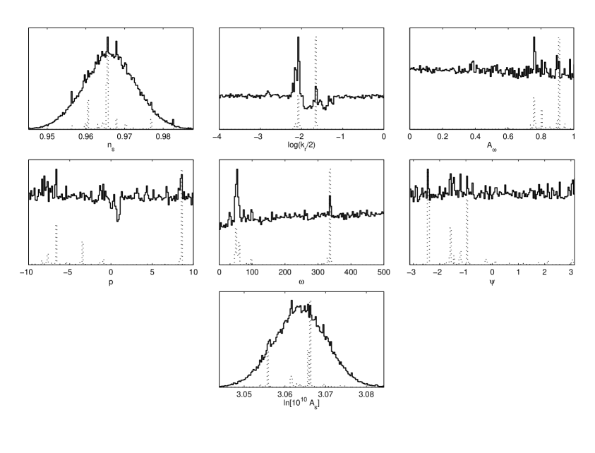
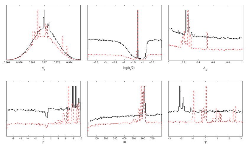
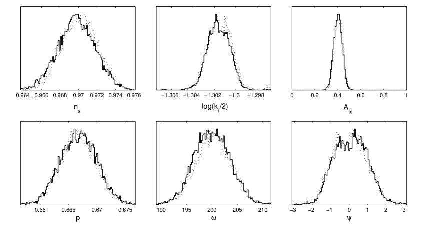
In Fig. 2, we have plotted the marginalized posterior probability distributions for the primordial parameters (solid curve). Both $A_{\scriptscriptstyle{\mathrm{S}}}$ and $n_{\scriptscriptstyle{\mathrm{S}}}$ are well constrained, as expected, and centered at the best fit values found by considering only a primordial power law spectrum [48]. The variance is somehow reduced, but this is the result of having fixed the cosmological parameters. On the other hand, all the other parameters exhibit flat distributions and therefore remain unconstrained. The dotted curves in this figure show the mean likelihood [53], which typically traces the location of the good fits. As discussed at length in Ref. [39, 55], the two distributions do not match when those better fits require some amount of fine-tuning between the parameters. Namely, they are located in small and correlated regions of the parameter space such that their integrated weight on the marginalized probability remains small. In Fig. 2, this situation appears for multiple values of the parameters. For instance, the distribution for $n_{\scriptscriptstyle{\mathrm{S}}}$ exhibit various “good fits” whereas the overall probability remains of Gaussian shape. The weight of each good fit can be assessed by the small deviation induced around the Gaussian distribution. Along these lines, the distribution of $\omega$ clearly exhibits two better fits for frequencies around $50$ and $300$, but the corresponding marginalized distribution does not peak by more than one sigma in these locations. In fact, these two frequencies are associated with the two favoured scales visible in the distribution of $k_{\mathrm{f}}$, which although not statistically significant, are clearly distinguishable. As we will see in the following, the scale $k_{\mathrm{f}}$ is actually the most sensitive parameter to the actual presence of a feature having a low signal-to-noise ratio.

The overall probability of having detected primordial fingerprints in the WMAP7 data is given by the posterior of $A_{\omega}$. Indeed, being marginalized over all the other parameters, it gives the probability density distribution of having a resonance of amplitude $A_{\omega}$, for all frequency, phase, location and power $p$. As one can check in Fig. 2, the $A_{\omega}$ posterior is mostly flat meaning that it is completely unconstrained. We conclude that there is no evidence for primordial fingerprints in the WMAP data. On the other hand, high values of $A_{\omega}$ are not disfavoured such that there is also no evidence against (up to the Occam’s razor favouring the simplest model [56]). This situation is in fact different than unlocalized primordial oscillations, such as those coming from non-standard vacuum initial conditions. In that case, large amplitudes are disfavoured because the oscillations are spread over all multipoles and, if too large, become incompatible with the observed signal [39, 55, 52]. Finally, in Fig. 2, one can notice that the posterior of $p$ is slightly reduced around small positive values. These models correspond to fast contraction, which, compared to the other expansion paradigms, have tendency to produce more widely spread oscillations in the $C_{\ell}$. As a result, too large amplitudes are not admissible and this region ends up being slightly disfavoured after marginalization. These models will be discussed in more details in Sec. 3.4.

In view of these results, it is instructive to discuss how much future CMB data can constrain the typical signal associated with features. In particular, do the peaks in the $k_{\mathrm{f}}$ distribution could be interpreted as hints of primordial fingerprints? In the next section, we present forecasts for an ideal Planck-like CMB experiment, using similar MCMC methods on mock data. We will see that $k_{\mathrm{f}}$ is indeed the most sensitive parameter to an underlying localized modulation. We will find out the minimum amplitude $A_{\omega}$ detectable for different fingerprints as we vary the frequency $\omega$ and fingerprint index $p$.

3 Planck-like CMB data

Figure 3: Temperature angular power spectrum, plus noise, for an inflationary feature (left panel) located at $\hat{k_{\mathrm{f}}}=0.05\,\mathrm{Mpc}^{-1}$, $\hat{A_{\omega}}=0.5$, $\hat{\omega}=600$, $\hat{p}=8$ (inflation) and $\hat{\psi}=0$. The right panel shows a feature at the same location but during a fast contracting era having $\hat{k_{\mathrm{f}}}=0.05\,\mathrm{Mpc}^{-1}$, $\hat{A_{\omega}}=0.4$, $\hat{\omega}=200$, $\hat{p}=2/3$ (matter contraction) and $\hat{\psi}=0$ (see Sec. 3.4).

Given a fiducial set of cosmological parameters $\{\hat{\lambda}_{a}\}$, the easier method to forecast their expected errors would be to use the Fisher matrix formalism which merely consists as approximating the likelihood by a Gaussian around the best fit location [57]. However, as discussed in Refs. [39, 55, 38] the likelihood associated with superimposed oscillations in the $C_{\ell}$ is non-Gaussian and can be multi-valued such that Fisher matrix method can only be applied for a high signal-to-noise detection. For this reason, we prefer in the following a MCMC exploration based on mock data containing various fingerprint oscillatory patterns [38].

3.1 Mock power spectrum and likelihood

Forecasts can be made through an MCMC exploration of the parameter space provided one specifies the likelihood. The mock data $\{\hat{\boldsymbol{C}}_{\ell}\}$ are assumed to be associated with a set of fiducial cosmological and primordial parameters $\{\hat{\lambda}_{a}\}$ and one needs to specify the likelihood of the theoretical $\{\boldsymbol{C}_{\ell}(\lambda_{a})\}$ tested. For a full sky analysis, assuming isotropic white noise for each pixel and Gaussian statistics, one can show that the sampling distribution followed by the $C_{\ell}$ is a Wishart distribution [58, 59, 60, 61]. Including polarization yields, up to a normalization constant [62]

$$-2\ln\mathcal{L}\!\left(\boldsymbol{D}_{\ell}|\hat{\boldsymbol{D}}_{\ell}\right)=\sum_{\ell}(2\ell+1)\left[\operatorname{Tr}\left(\hat{\boldsymbol{D}}_{\ell}\cdot\boldsymbol{D}_{\ell}^{-1}\right)-\ln\left|\hat{\boldsymbol{D}}_{\ell}\cdot\boldsymbol{D}_{\ell}^{-1}\right|-3\right].$$ (3.1)

The matrix $\boldsymbol{D}_{\ell}=\{D_{\ell}^{XY}\}$ where $X$, $Y$ stand for temperature and polarization variables, $T$, $E$ and $B$. The spectra $D_{\ell}^{XY}$ include a white noise component compared to the angular power spectra $C_{\ell}^{XY}$ and are defined by

$$D^{XY}_{\ell}\equiv C^{XY}_{\ell}+\dfrac{C_{\mathrm{noise}}^{X}}{(B^{X}_{\ell})^{2}}\,,$$ (3.2)

where $B^{X}_{\ell}$ is the beam response. For a Planck-like experiment, we have chosen a Gaussian beam with a full width at half maximum (fwhm) of $7^{\prime}$. The noise power for temperature has been set to $C_{\mathrm{noise}}^{T}=2\times 10^{-4}\,\mu\mathrm{K}^{2}$ and for polarization to $C_{\mathrm{noise}}^{E}\simeq C_{\mathrm{noise}}^{B}\simeq 2C_{\mathrm{noise}}^{T}$ [63]. From our modified version of the CAMB code, and the above noise specification, the $D^{XY}_{\ell}$ can be computed for any input value of the cosmological and primordial parameters $\{\lambda_{a}\}$. Two examples of the temperature angular power spectrum are represented in Fig. 3. Note that the oscillation amplitudes are greatly reduced in the temperature angular power spectrum comparing to those in the primordial power spectrum.

Using MCMC sampling with the likelihood of Eq. (3.1) allows to extract the posterior probability distribution for each “measured” parameter $\lambda_{a}$ given the fiducial model $\{\hat{\lambda}_{a}\}$. For the same reasons discussed in Sec. 2, we have fixed the cosmological parameters to their best fit value, obtained from a standard power-law primordial power spectrum, and ran the MCMC exploration only in the primordial parameter space. The standard cosmological fiducial parameters are the same as in Sec. 2, plus $\hat{n_{\scriptscriptstyle{\mathrm{S}}}}=0.97$ and $\ln(10^{10}\hat{A_{\scriptscriptstyle{\mathrm{S}}}})=3.166$. In the following, we consider various fiducial values for the fingerprint parameters and discuss how well they can be reconstructed.

3.2 No feature: the sensitivity zone

Figure 4: Marginalized posterior probability distributions for the primordial parameters (solid), and mean likelihood (dotted), associated with the mock Planck-like data when there is not any feature present. Notice the posterior of $k_{\mathrm{f}}$ which inversely traces the feature sensitivity region.

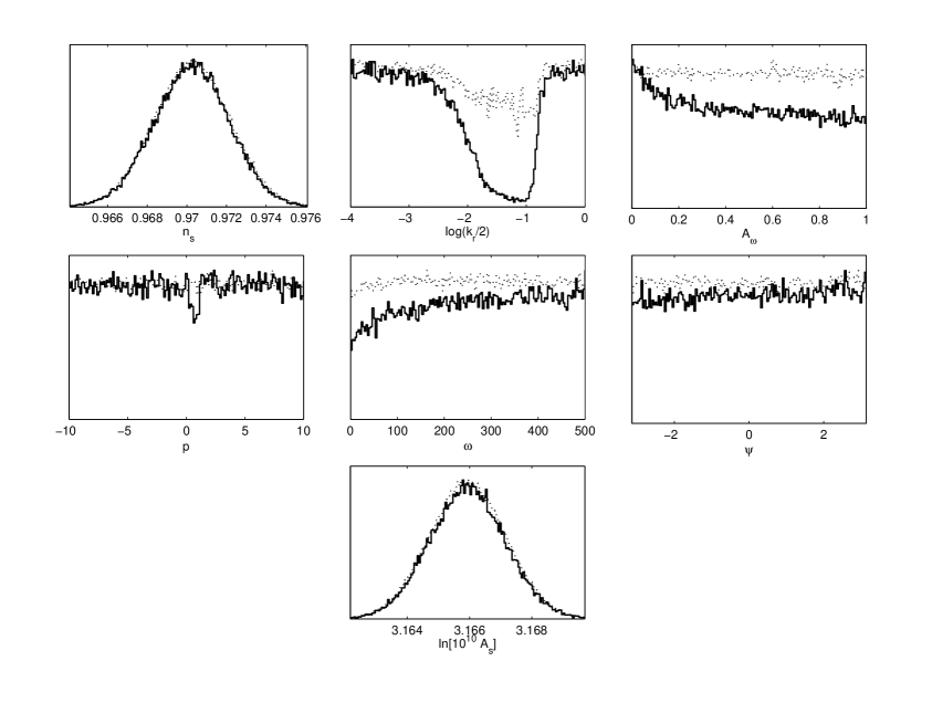
The first fiducial model considered has no feature, i.e. $\hat{A_{\omega}}=0$. Practically, the MCMC chains are run as specified in Sec. 2, with the same convergence criteria, i.e. the chains are stopped when the expected error on the marginalized distributions does not exceed a few percents. In Fig. 4, we have represented the marginalized posterior distributions obtained from the MCMC exploration of the primordial parameter space.

Figure 5: One- and two-sigma confidence intervals in the planes $(\log k_{\mathrm{f}},A_{\omega})$ and $(\log k_{\mathrm{f}},\omega)$ and mean likelihood (shading) for vanishing fingerprints in the mock data. These domains trace the sensitivity region of Planck-like CMB data. For $k_{\mathrm{f}}\gtrsim 10^{-1}\,\mathrm{Mpc}^{-1}$ or $k_{\mathrm{f}}\lesssim 10^{-2}\,\mathrm{Mpc}^{-1}$, localized resonances are hardly detectable.

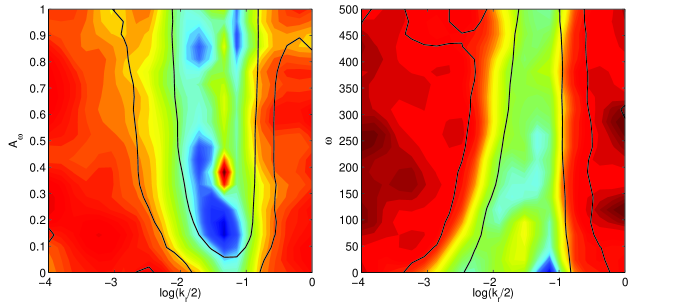
The distribution for the standard primordial parameters, $n_{\scriptscriptstyle{\mathrm{S}}}$ and $A_{\scriptscriptstyle{\mathrm{S}}}$, are reconstructed, as expected for well constrained parameters. Almost all fingerprint parameters exhibit a flat distribution and are unconstrained. The slight deviations between mean likelihood and marginalized posteriors for $A_{\omega}$, $\omega$ and $k_{\mathrm{f}}$ are the signatures of correlations. In Fig. 5, we have plotted the two-dimensional one- and two-sigma confidence intervals as well as the two-dimensional mean likelihood (shading). This plot shows that there is a strongly disfavoured region for $k_{\mathrm{f}}$ between $10^{-2}\,\mathrm{Mpc}^{-1}$ and $10^{-1}\,\mathrm{Mpc}^{-1}$. In this domain, Planck-like data are sensitive to the presence of features and as our fiducial model has no feature, this region is disfavoured. Conversely, the other domains are poorly constrained. On smaller scales the noise starts to dominate whereas on larger scales any resonance pattern is smoothed out by the CMB transfer functions [39, 55]. The one-dimensional distributions of Fig. 4 end up being flat because, for any $A_{\omega}$ (or $\omega$) value, there exists a scale $k_{\mathrm{f}}$ for which the model can be made undetectable within a Planck-like accuracy CMB experiment.

3.3 Fingerprints of inflation

As a starting point, we consider an inflation model with $\hat{p}=8$, having a strong feature of amplitude $\hat{A_{\omega}}=0.5$, at a high frequency $\hat{\omega}=600$, and located in the middle of the detectable zone, i.e. $\hat{k_{\mathrm{f}}}=0.05\,\mathrm{Mpc}^{-1}$ ($\psi=0$). Such a model has an angular temperature power spectrum represented in Fig. 3 (the polarization spectra are not represented but exhibit a similar behaviour).

Figure 6: Marginalized posterior probability distributions for the primordial parameters (solid), and mean likelihood (dotted), for typical Planck-like mock CMB data having a feature with $\hat{A_{\omega}}=0.5$, $\hat{\omega}=600$, $\hat{\psi}=0$, $\hat{p}=8$ and $\hat{k_{\mathrm{f}}}=0.05\,\mathrm{Mpc}^{-1}$ (same as in Fig. 3). Being in the high sensitivity zone, all fingerprint parameters are well reconstructed, especially the scale $k_{\mathrm{f}}=k_{\mathrm{r}}/2$. For such a strong signal, the fingerprint parameter $p$ can even be precisely measured, in addition to the conclusion that $|p|>1$.

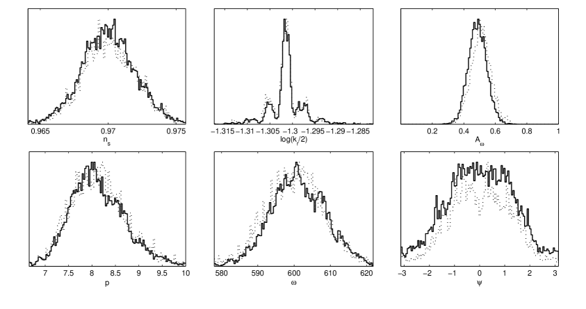
Running a MCMC exploration on the primordial parameters against such a model yields the marginalized distributions of Fig. 6. The power spectrum amplitude $A_{\scriptscriptstyle{\mathrm{S}}}$ is always well-constrained and its posterior remains identical to the one of Fig. 4. It is not represented in the following. The phase $\psi$ is poorly recovered whereas all the other fingerprint parameters are well determined. Their standard deviation are $\Delta A_{\omega}=0.08$, $\Delta\omega=43$, $\Delta\Psi=1.2$ and $\Delta p=2.9$ showing that such a feature would indeed allow to probe the expansion rate through $p$. The most sensitive parameter remains however the wavenumber scale as we find its standard deviation to be $\Delta k_{\mathrm{f}}/k_{\mathrm{f}}=4\times 10^{-3}$.

Figure 7: Marginalized posteriors obtained by reducing the feature amplitude to $\hat{A_{\omega}}=0.4$ (red dashed) and $\hat{A_{\omega}}=0.3$ (black solid). The other parameters are the same as in Fig. 6. Already for $\hat{A_{\omega}}=0.4$, the posterior for $A_{\omega}$ gets noisy showing that such a feature is no longer detectable. However, frequency and scale are still felt and are the most sensitive parameters. Amplitude, phase and the expansion parameter $p$ requires a stronger signal to be inferred (see Fig. 6).

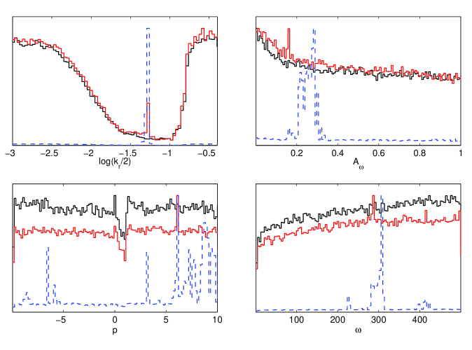
In order to test the sensitivity of Planck-like CMB data with respect to the amplitude, we have redone the same analysis for various fiducial amplitudes $\hat{A_{\omega}}$, all the other fiducial primordial parameters being unchanged. The marginalized posteriors are represented in Fig. 7 and shows that for $\hat{A_{\omega}}\lesssim 0.4$, any detection becomes unlikely and impossible for $\hat{A_{\omega}}<0.3$. Let us notice that already for $\hat{A_{\omega}}=0.4$, amplitude, phase and the expansion parameter $p$ are poorly, if not recovered. This suggests that, for a high frequency fingerprint, the presence of a strong feature, as the one discussed previously, is crucial for probing the $p$ parameter. There exists a very sharp line in terms of the value of $\hat{A_{\omega}}$ between the signals that can be reconstructed and those cannot. On the other hand, the parameters such as the frequency $\omega$ and the feature scale $k_{\mathrm{f}}$ still let some imprints, down to $\hat{A_{\omega}}=0.3$.

Figure 8: Same as Fig. 7 but for a reduced frequency $\hat{\omega}=300$. The sensitivity is slightly increased as signals down to $\hat{A_{\omega}}\simeq 0.3$ are now detectable in the posterior for $A_{\omega}$. Only the constrained fingerprint parameters are represented for three fiducial amplitudes $\hat{A_{\omega}}=0.3$ (dashed blue), $\hat{A_{\omega}}=0.2$ (solid red) and $\hat{A_{\omega}}=0.1$ (thick black).

The effect from changing the fiducial frequency in the mock data is typical of any other resonant pattern: the CMB transfer function smoothing out rapid oscillations, at constant $\hat{A_{\omega}}$, higher frequencies produce a lower signal in the CMB [37]. In Fig. 8, we have plotted the posteriors obtained for a fiducial model having $\hat{\omega}=300$ and for various values of the amplitude $\hat{A_{\omega}}$. The behaviour is exactly the same as for $\hat{\omega}=600$, but the sensitivity to $\hat{A_{\omega}}$ is increased because the resonances are less smoothed out by the CMB transfer function. So signals with lower amplitudes become slightly more accessible.

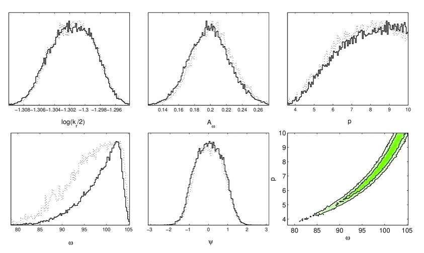
We have further tested examples with relatively low frequencies. In Fig. 9 we have shown the posteriors for an underlying fingerprint with $\hat{w}=100$ and $\hat{A_{\omega}}=0.2$. We can see that, for low frequency, a fingerprint would be detected by Planck with much lower amplitude. For example, the posterior for $A_{\omega}$ is sharply peaked at the fiducial value with a standard deviation of $\Delta A_{\omega}=0.03$. While most of the parameters can be reconstructed as before, there is an interesting exception of the posterior of $p$. This parameter can now only be constrained from below: $p>5$ at $95\%$ of confidence. The loss of accuracy on $p$ also affects the determination of $\omega$ as both parameters are degenerated (see the two-dimensional posterior in Fig. 9). This is not difficult to explain. In the large $|p|$ limit, the fingerprint profile approaches to a unique de Sitter limit, so fingerprints with large $p$ values tend to be degenerate. With lower frequency, this degeneracy becomes more effective since the “standard clock” is running slower and there are fewer “ticks” available to reconstruct the exact parameter $p$. However for our purpose, the exact value of $p$ is not the most important one. As long as we can demonstrate $|p|\gg 1$, we would be able to identify the inflation as the underlying paradigm. Interestingly, Fig. 9 shows that the posterior for $p$ indeed unambiguously indicates that this is an inflationary paradigm, although recovering $\hat{p}=8$ is no longer possible. We have also tested a lower frequency signal having $\hat{\omega}=50$ (and $\hat{A_{\omega}}=0.2$, figures not represented). The posteriors are very similar to those of Fig. 9, the amplitude and frequency are peaked at their fiducial value. The exact $p$ value cannot be reconstructed as well, and now the degeneracies between $(\omega,p)$ are extended to negative $p$ values (including the other inflationary branch $p<-1$). The bound for inflation, $|p|>1$, can still be established but by not more than two-sigma as the $99\%$ confidence region includes other paradigms. Further lowering the frequency however will not help to reduce the minimum detectable amplitude. This is because, with fewer oscillations, the fingerprints start to be confused with the acoustic oscillations. They sometimes do not even appear as oscillations, but only as deformations of various acoustic peaks.

Figure 9: Posteriors obtained with a small inflationary feature at low frequency: $\hat{A_{\omega}}\simeq 0.2$ and $\hat{\omega}=100$. Although low frequencies render smaller oscillation amplitude detectable, the $p$ value cannot be reconstructed but still indicates an inflationary paradigm. At lower frequencies, for instance $\hat{A_{\omega}}=50$, the posterior of $p$ extends to negative values such that distinguishing the inflationary paradigm from another expansion era becomes more difficult (see text). The lower right panel shows the one- and two-sigma confidence intervals of two-dimensional posterior in the plane $(\omega,p)$: the two parameters are correlated.

Figure 10: Primordial posteriors for an expanding model having $\hat{p}=-2$, with $\hat{A_{\omega}}=0.5$ and $\hat{\omega}=300$. The expansion parameter $p$ is recovered at a standard deviation of $\Delta p=0.15$.

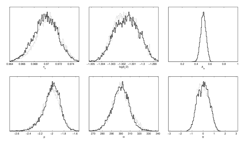
In order to explore different possibilities, we have also tested a rather unusual inflation model with $\hat{p}=-2$ and $\hat{\omega}=300$, all the other fiducial parameters being as before. This is still inflation in the sense that $|p|>1$, but unusual because the expansion rate is much slower than the de Sitter space and the Hubble parameter is increasing. As Eq. (1.1) shows, the $k$-dependency is such that the “instantaneous” frequency decreases faster than a logarithm for $k/k_{\mathrm{f}}\gg 1$. From the CMB point of view, it means that the signal is less damped by the transfer functions and the oscillatory pattern is spread over larger multipoles than for the inflationary paradigm ($p\gg 1$). In Fig. 10, we have represented the marginalized posteriors obtained by a MCMC analysis. Compared to the case $\hat{p}=8$, fingerprint parameters are more constrained due to the larger CMB signal, this is particularly clear for the phase $\psi$. Varying amplitude and frequency reproduces the same qualitative behaviour discussed before, namely one would find that all features disappear for $\hat{A_{\omega}}<0.1$. Again, $k_{\mathrm{f}}$ remains the most sensitive parameter as we find his posterior well peaked down to $\hat{A_{\omega}}=0.2$.

3.4 Beyond the inflationary paradigm

In this section, we discuss the detectability of the fingerprints within alternatives to inflation. We consider three categories: slow-contraction models ($0<p\ll 1$), slow-expansion models ($-1\ll p<0$) and fast-contraction models ($p\lesssim 1$). Fast-expanding but non-inflationary cases ($-1<p<0$ and $p\sim-1$) are similar to the $\hat{p}=-2$ case considered in the previous section.

Figure 11: Two types of undetectable features for a Planck-like experiment. Left panel: zoom on the second and third acoustic peaks for a slow contracting model $\hat{p}=0.1$, $\hat{A_{\omega}}=0.5$ and $\hat{\omega}=6000$. The resonances are before the feature scale $k_{\mathrm{f}}=0.05\,\mathrm{Mpc}^{-1}$ but remain very localized due to the small value of $p$. Right panel: an inflation model, $\hat{p}=8$, having a strong feature $\hat{A_{\omega}}=0.8$ washed out under cosmic variance by the large scale CMB transfer functions. It has $k_{\mathrm{f}}=0.01\,\mathrm{Mpc}^{-1}$ and $\hat{\omega}=300$ (see Sec. 3.5).

To test the slowly contracting models, we consider the case $\hat{p}=0.1$. The effective resonance frequency being given by $\omega p^{2}$, superimposed oscillatory patterns end up being of observable frequency for $\omega\gg 1/p^{2}$. For this reason, we have considered a fiducial model having $\hat{\omega}=6000$, its temperature angular power spectrum is represented in Fig. 11 for $\hat{A_{\omega}}=0.5$. The small value of $p$ makes the oscillation pattern very localized around $k_{\mathrm{f}}$ and this model ends up being unobservable. Even for an unrealistic maximal modulation amplitude ($\hat{A_{\omega}}=1$), the MCMC analysis does not allow the reconstruction of any fingerprint parameters.

The case of slowly expanding models is very close, their fingerprints exhibit similarity to the slowly contracting models which would affect their detectability (see the last two figures in Fig. 1).

Figure 12: Expected marginalized posteriors for a feature generated during a fast contracting era and having $\hat{A_{\omega}}=0.4$, $\hat{\omega}=200$, $\hat{p}=2/3$ (the temperature power spectrum is plotted in Fig. 3).

Faster contracting models, having larger values of $\hat{p}$, should not suffer from this problem, as for instance a matter contraction with $\hat{p}=2/3$. On the contrary, they exhibit widespread oscillations in the primordial power spectra for $k<k_{\mathrm{f}}$ but, as seen in Eq. (1.1), their “instantaneous” frequency increases dramatically. Depending on the values of $k_{\mathrm{f}}$, if the frequency $\omega$ becomes too large, the CMB transfer functions acting as a low-pass filter strongly damp the oscillatory tail at large multipoles. As a result, the fingerprints may no longer be visible above some $\ell$ value, which could be lower than $\ell_{\mathrm{f}}$, thereby rendering parameter reconstruction difficult. These models can therefore be “visible” only for not too large frequencies, but this also implies the existence of a few oscillations in the $C_{\ell}$ having a stronger amplitude than for inflation. This is illustrated in the right panel of Fig. 3 where we have plotted the angular power spectrum associated with the feature $\hat{\omega}=200$ and $\hat{A_{\omega}}=0.4$. The resonance patterns show up at the top of the first peak whereas the feature scale is located at much smaller scales $\ell_{\mathrm{f}}\simeq 700$. In fact, such a characteristic explains why those models are a bit disfavoured by the WMAP7 data: compared to other early universe paradigms, at same amplitude and frequency, those $p$ values are associated with slightly too large oscillations in the $C_{\ell}$. Concerning the Planck forecasts, we have represented in Fig. 12 the posteriors obtained from the MCMC analysis. For the same fiducial amplitude $\hat{A_{\omega}}=0.4$, all parameters are well reconstructed and in particular the expansion index $p$. The above-mentioned sensitivity to the model parameters renders smaller amplitudes hardly detectable for Planck-like data. We have tested a smaller fiducial amplitude of $\hat{A_{\omega}}=0.3$ (figures not represented) for which the posterior of $A_{\omega}$ appears very noisy and not clearly peaked. However, and contrary to the inflation paradigms, the posterior of $p$ still indicates a contracting model because, even noisy, the oscillatory patterns remain typical of a fast contracting background. In that situation, $p$ ends up being a more sensitive parameter than the amplitude. For $\hat{A_{\omega}}\lesssim 0.2$, all hints for a signal are lost and the posteriors are identical to those of Fig. 4.

3.5 Outside the sensitivity zone

As one may expect, if the primordial feature occurs at a scale $k_{\mathrm{f}}$ which is well outside the sensitivity region, it cannot produce a large enough signal in the CMB to be clearly distinguished. To check how the transition occurs, we have performed a MCMC exploration for the same fiducial model as in Sec. 3.3 ($\hat{p}=8$, $\hat{\omega}=300$) but with a scale $k_{\mathrm{f}}=0.01\,\mathrm{Mpc}^{-1}$. Even for an amplitude $\hat{A_{\omega}}=0.8$, the marginalized posteriors for all primordial parameters are identical to those of Fig. 4, i.e. as if no feature were present. As explained before, this is the result of the strong smoothing by the CMB transfer functions, which are very efficient on the largest scales. Such a smoothing is visible on the fiducial power spectra as the resonance patterns remain under the cosmic variance (see right panel of Fig. 11). Let us mention that not increasing the numerical accuracy for the transfer functions, i.e. using CAMB at its default numerical precision, may produce spurious enhanced signals in the CMB [37].

Figure 13: Marginalized posteriors for a feature occurring at the small scale boundary of the sensitivity zone, $k_{\mathrm{f}}=0.1\,\mathrm{Mpc}^{-1}$. Most of the fingerprint parameters are very well reconstructed but not $p$ and $\omega$ which are strongly degenerated. Their respective one- and two-sigma confidence intervals are plotted in the rightmost lower frame. This is the result of the noise amputating some part of the oscillatory tail. Notice that the inflationary paradigm can still be inferred as $|p|>1$.

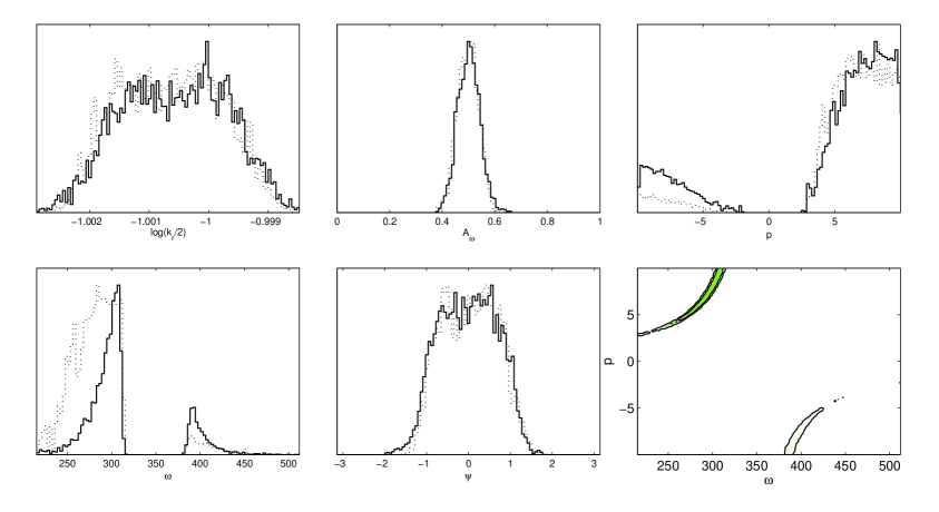
At smaller scales, the noise dominates. In Fig. 13, we have represented the posteriors obtained when the feature lies at the small scales boundary of the sensitivity domain, i.e. for $k_{\mathrm{f}}=0.1\,\mathrm{Mpc}^{-1}$ ($\ell_{\mathrm{f}}\simeq 1400$) and for $\hat{p}=8$, $\hat{A_{\omega}}=0.5$, $\hat{\omega}=300$. There is a net signal detection, the posterior of $A_{\omega}$ is sharply peaked around the expected fiducial value ($\Delta A_{\omega}=0.04$), as well for the scale $k_{\mathrm{f}}$ ($\Delta k_{\mathrm{f}}/k_{\mathrm{f}}=9\times 10^{-4}$). However, the frequency probability distribution appears to be multi-valued as well as the one for the expansion parameter $p$. In the same figure, we have plotted the one- and two-sigma confidence intervals associated with the two-dimensional posterior probability distribution in the plane $(\omega,p)$. Both parameters end up being strongly correlated as all shaded value provide a good fit to the CMB resonance pattern. This is reminiscent with the degeneracy mentioned previously when the frequency of an inflationary fingerprint is low. Here, compared to the same feature in the sensitivity zone, part of the oscillatory tail is actually truncated as becoming of smaller amplitude than the noise (see Fig. 3). As a result, there are less measurable “ticks” in the CMB and all combination of $p$ and $\omega$ producing similar oscillations around $k_{\mathrm{f}}$ cannot be distinguished. It is therefore not surprising that the posteriors obtained here are similar to the ones of Fig. 9. Let us notice that the data still “see” that this is an inflationary era – the oscillations remain on the right side of $k_{\mathrm{f}}$, independently of the truncation, and the posterior for $p$ is non-vanishing only when $|p|>1$. Further out of the sensitivity zone, the fingerprint signals remain undetectable.

4 Conclusions and discussions

We have studied the detectability of the fingerprints induced by standard clocks in various primordial universe paradigms. Concentrating on the power spectrum, we have found that they are detectable in Planck-like data provided they lie in the sensitivity zone $10^{-2}\,\mathrm{Mpc}^{-1}\lesssim\hat{k_{\mathrm{f}}}\lesssim 10^{-1}\,\mathrm{Mpc}^{-1}$. The scale $k_{\mathrm{f}}$, and frequency $\omega$ are the most sensible parameter to the actual presence of a fingerprint in the data in most cases. For inflation, although their posteriors exhibit characteristic signatures for an amplitude as small as $\hat{A_{\omega}}=0.1$ ($10\%$ modulation), we have shown that a proper reconstruction of the parameter $p$ requires a higher signal $\hat{A_{\omega}}\gtrsim 0.5$, especially at high frequencies ($\omega\gtrsim 300$). The situation is however improved at lower frequency ($\omega\simeq 100$) as amplitudes $\hat{A_{\omega}}\gtrsim 0.2$ still allow to infer the inflationary paradigm $|p|>1$. Alternatives to inflation with small $|p|\ll 1$ have been found to deviate from this rule as very small value of $\hat{p}$ end up being more difficult to detect. As discussed in the previous sections, this is essentially due to how widespread the observable oscillatory patterns are. In any case, the high sensitivity zone in $k_{\mathrm{f}}$ is the region to explore with the soon to be released Planck data.

We have also seen that, for inflation, establishing the bound $|p|>1$ is easier than a full reconstruction of the index $p$. So the main strength of the standard clocks is to break the leading degeneracy between the paradigms with $|p|>1$ and $|p|<1$, especially if they predict degenerated power spectrum and non-Gaussianities in the absence of the fingerprints. Once this degeneracy is broken, the more precise value of $p$ could be inferred from other more standard observables such as the spectral index.

Most likely, hints for a feature could show up while not allowing a full reconstruction with the CMB power spectrum only. However, these standard clocks also imprint correlated signals in non-Gaussianities [6, 7]. These signals appear as leading order large non-Gaussianities instead of small corrections, due to the resonant mechanism [22]. The search for such scale-dependent and non-separable non-Gaussianities is a much more difficult task however (see e.g. Ref. [64, 65, 66] for possible methods). An efficient approach would be to search them first in the power spectrum, as we discuss in this paper. If any candidate signals are found, the locations of the corresponding non-Gaussianities will be determined, and the subsequent search for non-Gaussianities would be considerably narrowed down and provide non-trivial checks.

Finally, let us mention that the matter power spectrum, in the linear regime, is far less smoothed than the CMB concerning the transfer of features. However, those resonances are completely washed out by the galaxy survey window functions [37]. A possible future work, however, may be to discuss how much structure formation may be affected by features in the non-linear regime [67].

References

- [1] A. H. Guth, The inflationary universe: A possible solution to the horizon and flatness problems, Phys. Rev. D23 (1981) 347–356.
- [2] A. D. Linde, A new inflationary universe scenario: A possible solution of the horizon, flatness, homogeneity, isotropy and primordial monopole problems, Phys. Lett. B108 (1982) 389–393.
- [3] A. Albrecht and P. J. Steinhardt, Cosmology for grand unified theories with radiatively induced symmetry breaking, Phys. Rev. Lett. 48 (1982) 1220–1223.
- [4] Supernova Cosmology Project Collaboration, S. Perlmutter et. al., Discovery of a supernova explosion at half the age of the Universe and its cosmological implications, Nature 391 (1998) 51–54, [astro-ph/9712212].
- [5] Supernova Search Team Collaboration, A. G. Riess et. al., Observational evidence from supernovae for an accelerating universe and a cosmological constant, Astron.J. 116 (1998) 1009–1038, [astro-ph/9805201].
- [6] X. Chen, Primordial Features as Evidence for Inflation, JCAP 1201 (2012) 038, [arXiv:1104.1323].
- [7] X. Chen, Fingerprints of Primordial Universe Paradigms as Features in Density Perturbations, Phys.Lett. B706 (2011) 111–115, [arXiv:1106.1635].
- [8] R. Brandenberger, Do we have a Theory of Early Universe Cosmology?, arXiv:1204.6108.
- [9] J.-L. Lehners, Cosmic Bounces and Cyclic Universes, Class.Quant.Grav. 28 (2011) 204004, [arXiv:1106.0172].
- [10] T. Battefeld and S. Watson, String gas cosmology, Rev.Mod.Phys. 78 (2006) 435–454, [hep-th/0510022].
- [11] J. A. Adams, B. Cresswell, and R. Easther, Inflationary perturbations from a potential with a step, Phys.Rev. D64 (2001) 123514, [astro-ph/0102236].
- [12] X. Chen, R. Easther, and E. A. Lim, Large Non-Gaussianities in Single Field Inflation, JCAP 0706 (2007) 023, [astro-ph/0611645].
- [13] A. Achucarro, J.-O. Gong, S. Hardeman, G. A. Palma, and S. P. Patil, Features of heavy physics in the CMB power spectrum, JCAP 1101 (2011) 030, [arXiv:1010.3693].
- [14] P. Adshead, W. Hu, C. Dvorkin, and H. V. Peiris, Fast Computation of Bispectrum Features with Generalized Slow Roll, Phys.Rev. D84 (2011) 043519, [arXiv:1102.3435]. 14 pages, 9 figures, typos fixed.
- [15] W. Hu, Generalized Slow Roll for Non-Canonical Kinetic Terms, Phys.Rev. D84 (2011) 027303, [arXiv:1104.4500].
- [16] F. Arroja, A. E. Romano, and M. Sasaki, Large and strong scale dependent bispectrum in single field inflation from a sharp feature in the mass, Phys.Rev. D84 (2011) 123503, [arXiv:1106.5384].
- [17] Z. Huang, L. Verde, and F. Vernizzi, Constraining inflation with future galaxy redshift surveys, JCAP 1204 (2012) 005, [arXiv:1201.5955]. a few reference changed in v2.
- [18] F. Arroja and M. Sasaki, Strong scale dependent bispectrum in the Starobinsky model of inflation, arXiv:1204.6489.
- [19] A. Avgoustidis, S. Cremonini, A.-C. Davis, R. H. Ribeiro, K. Turzynski, et. al., Decoupling Survives Inflation: A Critical Look at Effective Field Theory Violations During Inflation, arXiv:1203.0016. 42 Pages and 2 figures, references added.
- [20] S. Cespedes, V. Atal, and G. A. Palma, On the importance of heavy fields during inflation, JCAP 1205 (2012) 008, [arXiv:1201.4848].
- [21] A. A. Abolhasani, H. Firouzjahi, S. Khosravi, and M. Sasaki, Local Features with Large Spiky non-Gaussianities during Inflation, arXiv:1204.3722.
- [22] X. Chen, R. Easther, and E. A. Lim, Generation and Characterization of Large Non-Gaussianities in Single Field Inflation, JCAP 0804 (2008) 010, [arXiv:0801.3295].
- [23] R. Bean, X. Chen, G. Hailu, S.-H. H. Tye, and J. Xu, Duality Cascade in Brane Inflation, JCAP 0803 (2008) 026, [arXiv:0802.0491].
- [24] R. Flauger, L. McAllister, E. Pajer, A. Westphal, and G. Xu, Oscillations in the CMB from Axion Monodromy Inflation, JCAP 1006 (2010) 009, [arXiv:0907.2916].
- [25] R. Flauger and E. Pajer, Resonant Non-Gaussianity, JCAP 1101 (2011) 017, [arXiv:1002.0833].
- [26] X. Chen, Folded Resonant Non-Gaussianity in General Single Field Inflation, JCAP 1012 (2010) 003, [arXiv:1008.2485].
- [27] L. Leblond and E. Pajer, Resonant Trispectrum and a Dozen More Primordial N-point functions, JCAP 1101 (2011) 035, [arXiv:1010.4565].
- [28] S. R. Behbahani, A. Dymarsky, M. Mirbabayi, and L. Senatore, (Small) Resonant non-Gaussianities: Signatures of a Discrete Shift Symmetry in the Effective Field Theory of Inflation, arXiv:1111.3373.
- [29] M. Aich, D. K. Hazra, L. Sriramkumar, and T. Souradeep, Oscillations in the inflaton potential: Exact numerical analysis and comparison with the recent and forthcoming CMB datasets, arXiv:1106.2798.
- [30] J. C. Niemeyer, Inflation with a high frequency cutoff, Phys. Rev. D63 (2001) 123502, [astro-ph/0005533].
- [31] J. Martin and R. H. Brandenberger, The trans-planckian problem of inflationary cosmology, Phys. Rev. D63 (2001) 123501, [hep-th/0005209].
- [32] R. Easther, B. R. Greene, W. H. Kinney, and G. Shiu, Inflation as a probe of short distance physics, Phys. Rev. D64 (2001) 103502, [hep-th/0104102].
- [33] R. Easther, B. R. Greene, W. H. Kinney, and G. Shiu, Imprints of short distance physics on inflationary cosmology, Phys. Rev. D67 (2003) 063508, [hep-th/0110226].
- [34] O. Elgaroy and S. Hannestad, Can Planck-scale physics be seen in the cosmic microwave background ?, Phys. Rev. D68 (2003) 123513, [astro-ph/0307011].
- [35] J. Martin and C. Ringeval, Superimposed Oscillations in the WMAP Data?, Phys. Rev. D69 (2004) 083515, [astro-ph/0310382].
- [36] N. Kaloper and M. Kaplinghat, Primeval corrections to the cmb anisotropies, Phys. Rev. D68 (2003) 123522, [hep-th/0307016].
- [37] J. Martin and C. Ringeval, Addendum to “Superimposed Oscillations in the WMAP Data?”, Phys. Rev. D69 (2004) 127303, [astro-ph/0402609].
- [38] R. Easther, W. H. Kinney, and H. Peiris, Observing trans-Planckian signatures in the cosmic microwave background, JCAP 0505 (2005) 009, [astro-ph/0412613].
- [39] J. Martin and C. Ringeval, Exploring the superimposed oscillations parameter space, JCAP 0501 (2005) 007, [hep-ph/0405249].
- [40] K. Schalm, G. Shiu, and J. P. van der Schaar, Decoupling in an expanding universe: Boundary RG flow affects initial conditions for inflation, JHEP 0404 (2004) 076, [hep-th/0401164].
- [41] J. Hamann, S. Hannestad, M. S. Sloth, and Y. Y. Wong, Observing trans-Planckian ripples in the primordial power spectrum with future large scale structure probes, JCAP 0809 (2008) 015, [arXiv:0807.4528].
- [42] F. T. Falciano, M. Lilley, and P. Peter, A Classical bounce: Constraints and consequences, Phys.Rev. D77 (2008) 083513, [arXiv:0802.1196].
- [43] M. Lilley, L. Lorenz, and S. Clesse, Observational signatures of a non-singular bouncing cosmology, JCAP 1106 (2011) 004, [arXiv:1104.3494].
- [44] C. Burgess, J. M. Cline, F. Lemieux, and R. Holman, Are inflationary predictions sensitive to very high-energy physics?, JHEP 0302 (2003) 048, [hep-th/0210233].
- [45] G. Shiu and J. Xu, Effective Field Theory and Decoupling in Multi-field Inflation: An Illustrative Case Study, Phys.Rev. D84 (2011) 103509, [arXiv:1108.0981]. 24 pages, 2 figures, references added.
- [46] X. Gao, D. Langlois, and S. Mizuno, Influence of heavy modes on perturbations in multiple field inflation, arXiv:1205.5275.
- [47] WMAP Collaboration Collaboration, L. Page et. al., First year Wilkinson Microwave Anisotropy Probe (WMAP) observations: Interpretation of the TT and TE angular power spectrum peaks, Astrophys.J.Suppl. 148 (2003) 233, [astro-ph/0302220].
- [48] WMAP Collaboration, E. Komatsu et. al., Seven-Year Wilkinson Microwave Anisotropy Probe (WMAP) Observations: Cosmological Interpretation, Astrophys. J. Suppl. 192 (2011) 18, [arXiv:1001.4538].
- [49] D. Larson et. al., Seven-Year Wilkinson Microwave Anisotropy Probe (WMAP) Observations: Power Spectra and WMAP-Derived Parameters, Astrophys. J. Suppl. 192 (2011) 16, [arXiv:1001.4635].
- [50] N. Jarosik et. al., Seven-Year Wilkinson Microwave Anisotropy Probe (WMAP) Observations: Sky Maps, Systematic Errors, and Basic Results, Astrophys. J. Suppl. 192 (2011) 14, [arXiv:1001.4744].
- [51] A. Lewis, A. Challinor, and A. Lasenby, Efficient computation of cmb anisotropies in closed frw models, Astrophys. J. 538 (2000) 473–476, [astro-ph/9911177].
- [52] P. D. Meerburg, R. Wijers, and J. P. van der Schaar, WMAP 7 Constraints on Oscillations in the Primordial Power Spectrum, arXiv:1109.5264.
- [53] A. Lewis and S. Bridle, Cosmological parameters from cmb and other data: a monte- carlo approach, Phys. Rev. D66 (2002) 103511, [astro-ph/0205436].
- [54] A. Gelman and D. Rubin, Inference from iterative simulations using multiple sequences, Statistical Science 7 (1992) 457–511.
- [55] J. Martin and C. Ringeval, Inflation after WMAP3: Confronting the slow-roll and exact power spectra to CMB data, JCAP 0608 (2006) 009, [astro-ph/0605367].
- [56] R. Trotta, Bayes in the sky: Bayesian inference and model selection in cosmology, Contemp.Phys. 49 (2008) 71–104, [arXiv:0803.4089].
- [57] M. Tegmark, A. Taylor, and A. Heavens, Karhunen-Loeve eigenvalue problems in cosmology: How should we tackle large data sets?, Astrophys.J. 480 (1997) 22, [astro-ph/9603021].
- [58] J. Bond, A. H. Jaffe, and L. Knox, Radical compression of cosmic microwave background data, Astrophys.J. 533 (2000) 19, [astro-ph/9808264].
- [59] L. Perotto, J. Lesgourgues, S. Hannestad, H. Tu, and Y. Y. Wong, Probing cosmological parameters with the CMB: Forecasts from full Monte Carlo simulations, JCAP 0610 (2006) 013, [astro-ph/0606227].
- [60] W. J. Percival and M. L. Brown, Likelihood methods for the combined analysis of CMB temperature and polarisation power spectra, Mon.Not.Roy.Astron.Soc. 372 (2006) 1104–1116, [astro-ph/0604547].
- [61] S. Hamimeche and A. Lewis, Likelihood Analysis of CMB Temperature and Polarization Power Spectra, Phys.Rev. D77 (2008) 103013, [arXiv:0801.0554].
- [62] L. Colombo, E. Pierpaoli, and J. Pritchard, Cosmological parameters after WMAP5: forecasts for Planck and future galaxy surveys, Mon.Not.Roy.Astron.Soc. 398 (2009) 1621, [arXiv:0811.2622].
- [63] PLANCK Collaboration, J.-M. Lamarre et. al., Planck pre-launch status: The HFI instrument, from specification to actual performance, Astronomy and Astrophysics 520 (2010) A9. LPSC10178, LAL 10-202.
- [64] J. R. Fergusson and E. P. S. Shellard, The shape of primordial non-Gaussianity and the CMB bispectrum, Phys. Rev. D80 (2009) 043510, [arXiv:0812.3413].
- [65] P. D. Meerburg, J. P. van der Schaar, and M. G. Jackson, Bispectrum signatures of a modified vacuum in single field inflation with a small speed of sound, JCAP 1002 (2010) 001, [arXiv:0910.4986].
- [66] M. Liguori, E. Sefusatti, J. R. Fergusson, and E. P. S. Shellard, Primordial non-Gaussianity and Bispectrum Measurements in the Cosmic Microwave Background and Large-Scale Structure, Adv. Astron. 2010 (2010) 980523, [arXiv:1001.4707].
- [67] L. Felippe S. Rodrigues and R. Opher, A large change in the predicted number of small halos due to a small amplitude oscillating inflaton potential, Phys. Rev. D82 (2010) 023501, [arXiv:1006.2159].