The oriented graph of multi-graftings in the Fuchsian case

Abstract.

We prove the connectedness and compute the diameter of the oriented graph of multi-graftings associated to exotic $\mathbb{CP}^{1}$-structures on a compact surface $S$ with a given holonomy representation of Fuchsian type.

1. Introduction

Let $\Gamma_{g}$ be the fundamental group of a compact oriented surface $S$ of genus $g\geq 2$, and $\rho:\Gamma_{g}\rightarrow\mathrm{PSL}(2,\mathbb{R})$ be a Fuchsian representation, namely a faithful and discrete one. A marked surface of genus $g$ is the data of a simply connected cover $\widetilde{S}$ of $S$ together with a free discontinuous action of $\Gamma_{g}$. A $\mathbb{CP}^{1}$-structure (sometimes referred to as a projective structure) with holonomy $\rho$ on the marked surface is a local diffeomorphism $D:\widetilde{S}\rightarrow\mathbb{CP}^{1}$ called developing map which is $\rho$-equivariant. We denote by $P(\rho)$ the set of equivalence classes of marked $\mathbb{CP}^{1}$-structures on a surface of genus $g$ with holonomy $\rho$, where two projective structures $(\widetilde{S_{i}},D_{i})$, $i=1,2$ are equivalent if there exists a $\Gamma_{g}$-equivariant diffeomorphism $\Phi:\widetilde{S_{1}}\rightarrow\widetilde{S_{2}}$ such that $D_{1}=D_{2}\circ\Phi$.

This article deals with the study of a surgery operation called grafting that produces, given an element in $P(\rho)$, new elements in the same set. Grafting consists in cutting a surface equipped with a $\mathbb{CP}^{1}$-structure along a particular type of simple closed curve called graftable curve, and gluing a Hopf annulus, namely the quotient of a simply connected domain of the Riemann sphere invariant by the (loxodromic) holonomy of the graftable curve. This operation produces a new element of $P(\rho)$.

Grafting was used by Hejhal [5, Theorem 4] and Thurston (unpublished) to produce examples of projective structures with holonomy $\rho$ that are different from the uniformizing structure $\sigma_{u}=\rho(\Gamma_{g})\backslash\mathbb{H}^{2}$. Such structures are called exotic. The importance of grafting comes from the fact that it allows to define coordinates on $\mathcal{P}(\rho)$ when $\rho$ is a Fuchsian representation: Goldman proved that any $\mathbb{CP}^{1}$-structure with holonomy $\rho$ is obtained from the uniformizing one by grafting a collection of disjoint graftable simple closed curves (see [4]). Such an operation will be called a multi-grafting.

The goal of this note is to improve Goldman’s result in the following way.

Theorem 1.1.

Let $\sigma_{1}$ and $\sigma_{2}$ be two exotic projective structures sharing the same Fuchsian holonomy. Then $\sigma_{2}$ can be obtained from $\sigma_{1}$ by a sequence of two multi-graftings.

A consequence of this result is that there exist positive cycles of graftings, namely finite sequences of marked $\mathbb{CP}^{1}$-structures $\sigma_{0},\ldots,\sigma_{r}=\sigma_{0}$ such that for each $i=1,\ldots,r$, $\sigma_{i}$ is a grafting of $\sigma_{i-1}$. The integer $r$ is then called the period of the cycle. Observe that an immediate corollary of the theorem is that any couple of exotic $\mathbb{CP}^{1}$-structures are contained in such a positive cycle of period bounded by $4$. We will see (Corollary 4.2) that indeed there are such cycles of period $2$.

Let $MG(\rho)$ be the oriented graph whose vertices are elements of $\mathcal{P}(\rho)$ and two vertices $\sigma_{1},\sigma_{2}$ are joined by an oriented edge from $\sigma_{1}$ to $\sigma_{2}$ if $\sigma_{2}$ is obtained from $\sigma_{1}$ by a multi-grafting. Theorem 1.1 can be restated by saying that the oriented graph of multi-graftings $MG(\rho)\setminus\sigma_{u}$ is a connected graph of radius $2$. As a consequence we also get that the fundamental group of $MG(\rho)$ is not finitely generated.

To prove the results we will use some surgery operations on multi-curves introduced by Luo [7] and later developed by Ito [6]. Our results and methods are closely related to Thompson’s, see [8], but he considers the case of Schottky representations instead of Fuchsian ones. We observe that our argument extends stricto sensu to the case of quasi-Fuchsian representations.

2. Graftable curves

In this section we introduce the action of grafting on $\mathcal{P}(\rho)$ and define the graph of multi-graftings.

2.1. Definition

Recall that a multi-curve on a surface $S$ is a finite disjoint union of simple closed curves none of which is homotopically trivial. Let $\sigma$ be a marked projective structure on a compact orientable surface $S$. A multi-curve is said to be graftable (in $\sigma$) if all of its components have loxodromic holonomy and the developing map is injective when restricted to a lift of any of those components in $\widetilde{S}$. The condition is independent of the choice of representative in the class $[\sigma]\in\mathcal{P}(\rho)$.

2.2. Grafting along graftable curves

If $\alpha=\{\alpha_{i}\}_{i\in I}$ is a graftable multi-curve, one can produce another marked projective structure, called the grafting along $\alpha$, and denoted $\text{Gr}(\sigma,\alpha)$. We recall the construction here. We cut the surface $\widetilde{S}$ along the lifts $\widetilde{\alpha_{i}}$’s of the curves $\alpha_{i}$’s, and glue to each of them a copy of $\mathbb{CP}^{1}\setminus\overline{D(\widetilde{\alpha_{i}}})$ using the developing map for the gluing. We then obtain a new surface denoted by $\widetilde{S^{\prime}}$, together with a new map $D^{\prime}:\widetilde{S^{\prime}}\rightarrow\mathbb{CP}^{1}$ which is defined by $D$ on $\widetilde{S}\setminus\pi^{-1}(\cup_{i}\alpha_{i})$ and by the identity on the spherical domains $\mathbb{CP}^{1}\setminus\overline{D(\widetilde{\alpha_{i}})}$. The $\Gamma_{g}$-action on $\widetilde{S}$ induces a $\Gamma_{g}$-action on $\widetilde{S^{\prime}}$ which is free and discontinuous, and the map $D^{\prime}$ is obviously $\rho$-equivariant. Hence, this defines a new marked projective structure $\text{Gr}(\sigma,\alpha)$ with holonomy $\rho$: the grafting of $\sigma$ over the graftable multi-curve $\alpha$.

As $\alpha_{i}$ has loxodromic holonomy, it acts freely and properly discontiuosly on $\mathbb{CP}^{1}\setminus\overline{D(\widetilde{\alpha_{i}})}$, and its quotient is a cylinder equipped with a projective structure. Therefore, the grafting can be viewed as a cut-and-paste procedure directly in $S$, which cuts $S$ along each $\alpha_{i}$ and glues back the cylinder $\langle\alpha_{i}\rangle\backslash(\mathbb{CP}^{1}\setminus\overline{D(\widetilde{\alpha_{i}})})$.

2.3. Isotopy class of graftable curves

It is an easy fact to verify that if $\alpha$ and $\alpha^{\prime}$ belong to the same connected component of the set of graftable multi-curves (for the compact open topology), then the resulting projective structures $\text{Gr}(\sigma,\alpha)$ and $\text{Gr}(\sigma,\alpha^{\prime})$ are equivalent. However, we will see that it can happen that $\alpha$ and $\alpha^{\prime}$ are two graftable multi-curves that are isotopic as multi-curves by an isotopy that leaves the space of graftable multi-curves, and such that their corresponding graftings are not equivalent (see Remark 3.4).

2.4. The graph of multi-graftings

Let $\rho$ be a representation from $\Gamma_{g}$ to $\mathrm{PSL}(2,\mathbb{C})$. Let us define the graph of multi-graftings $MG(\rho)$ in the following way. The vertices are the elements of $\mathcal{P}(\rho)$ and two of them $(S_{1},\sigma_{1})$ and $(S_{2},\sigma_{2})$ are the connected by a positive segment from $\sigma_{1}$ to $\sigma_{2}$ if there exists a graftable multi-curves $\alpha$ in $S_{1}$ such that $\mathrm{Gr}(\sigma_{1},\alpha)=\sigma_{2}$.

3. Fuchsian case: construction of graftable curves

Recall that a representation $\rho:\Gamma_{g}\rightarrow\mathrm{PSL}(2,\mathbb{R})$ is Fuchsian if it is discrete and faithful. In the sequel $\rho$ will always be assumed to be Fuchsian.

3.1. Goldman’s parametrization of $MG(\rho)$

We will denote by $\sigma_{u}$ the uniformizing structure on the surface $S_{u}:=\rho(\Gamma_{g})\backslash\mathbb{H}^{2}$, which is obtained by taking the quotient of $\mathbb{H}^{2}$ by the $\rho$-action of $\Gamma_{g}$ on $\mathbb{H}^{2}$. For this structure, the developing map is just the identity when identifying the universal cover of $S_{u}$ with $\mathbb{H}^{2}$, and in particular is injective. Hence, any simple closed curve on $S_{u}$ is a graftable curve. Hence in this case the space of graftable multi-curves and the space of multi-curves are the same. By the discussion in §2.3 the grafting $\text{Gr}(\sigma_{u},\alpha)$ depends only on the isotopy class of $\alpha$ as a multi-curve.

Goldman proved in [4] that every marked projective structure $\sigma$ with holonomy $\rho$ is obtained by grafting the structure $\sigma_{u}$ along a multi-curve $\alpha=\{\alpha_{i}\}_{i}$. Moreover, this family is unique, and can be reconstructed from $\sigma$ in the following way. For a Fuchsian projective structure $\sigma$, denote by $S^{\mathbb{R}}$ (resp. $S^{\pm}$) the quotient of $D^{-1}(\mathbb{RP}^{1})$ (resp. $D^{-1}(\mathbb{H}^{\pm})$) by the covering group $\Gamma_{g}$. Since $\rho$ is Fuchsian, it preserves the decomposition $\mathbb{CP}^{1}=\mathbb{H}^{+}\cup\mathbb{RP}^{1}\cup\mathbb{H}^{-}$, and thus $S^{\mathbb{R}}$ is an analytic real submanifold of $S$ separating $S$ in domains which are either positive or negative according they belong to $S^{+}$ or $S^{-}$. Goldman proved that the components of $S^{-}$ are necessarily annuli. The set of annuli is homotopic to a unique multi-loop $\alpha$ satisfying $\sigma=\text{Gr}(\sigma_{u},\alpha)$. To abridge notations we define $\text{Gr}_{\alpha}:=\text{Gr}(\sigma_{u},\alpha)$.

3.2. Homotopically transverse multi-curves

Let $\alpha=\{\alpha_{i}\}_{i\in I}$ and $\beta=\{\beta_{j}\}_{j\in J}$ be two multi-curves. They are homotopically transverse if the following conditions hold:

• for each $i\in I$ and $j\in J$, the curves $\alpha_{i}$ and $\beta_{j}$ are not homotopic

• they are transverse in the usual sense and

• The complement of $(\cup\alpha_{i})\cup(\cup\beta_{j})$ in $S$ has no bi-gon component.

3.3. Construction of graftable multi-curves

Given a multi-curve $\alpha=\{\alpha_{i}\}_{i\in I}$, a set of turning directions for $\alpha$ is an assignment to each curve $\alpha_{i}$ of a turning direction $T_{i}\in\{R,L\}$ (“Right” or “Left”) in such a way that any two parallel curves have the same turning direction.

In this paragraph we provide a construction that, given two homotopically transverse multi-curves $\alpha=\{\alpha_{i}\}_{i\in I}$ and $\beta=\{\beta_{j}\}_{j\in J}$, and a set $T=\{T_{i}\}$ of turning directions for $\alpha$, produces a multi-curve $\beta_{T}$ which is graftable in $\text{Gr}_{\alpha}$ and isotopic to $\beta$.

We begin by assuming that there are no parallel curves in the families $\alpha$ and $\beta$. In this case we can assume that the components of $\alpha$ and $\beta$ are simple closed geodesics in the uniformizing structure $\sigma_{u}$.

Recall that $\text{Gr}_{\alpha}$ is obtained by gluing $S_{u}\setminus\alpha$ with some grafting annuli. We will explain the construction of $\beta_{T}$ in each piece of this decomposition separately, beginning with the intersection of $\beta_{T}$ with $S_{u}\setminus\alpha$, and then construct the intersection of $\beta_{T}$ with the grafting annuli glued to $S_{u}\setminus\alpha$ to obtain $\text{Gr}_{\alpha}$.

The boundary of $S_{u}\setminus\alpha$ consists of two copies $\alpha_{i}^{\prime}$ and $\alpha_{i}^{\prime\prime}$ of each curve $\alpha_{i}$, and for each component $C$ of $S_{u}\setminus\alpha$, its boundary is a union of such components. We fix a small positive number $\varepsilon$, and for each $p\in\alpha_{i}\cap\beta\in\partial C$, we consider the point $p_{T}\in\partial C$ lying at distance $\varepsilon$ from $p$ to the side of $p$ indicated by $T_{i}$ with respect to the orientation induced on $\alpha_{i}$ by $C$. If we do this for all components of $S_{u}\setminus\alpha$, we get for each point $p\in\alpha_{i}\cap\beta$ a couple of distinct points $p^{\prime}\in\alpha_{i}^{\prime}$ and $p^{\prime\prime}\in\alpha_{i}^{\prime\prime}$ lying at distance $\varepsilon$ from $p$ (as seen as a point in $\alpha_{i}$ or $\alpha_{i}^{\prime\prime}$ under the natural identifications $\alpha_{i}\simeq\alpha_{i}^{\prime}\simeq\alpha_{i}^{\prime\prime}$).

Now, $\beta\cap C$ is a union of geodesic segments $[p,q]$ joining points of $\partial C$. We define $\beta_{T}$ in $S_{u}\setminus\alpha\subset S$ to be the union of the segments $[p_{T},q_{T}]$ with $p_{T}$ and $q_{T}$ constructed as above. Observe that if we move the points $p,q$ a little bit, then the segments $[p_{T},q_{T}]$ are disjoint in the component $C$, but also in the whole surface $S$.

Then, one has to define the curve $\beta_{T}$ in the grafting annuli in a graftable way. The continuation should start from the point $p^{\prime}$ above and end at $p^{\prime\prime}$. (In Figure 1 we depicted the case $T_{i}=L$.)

Figure 1. The curve $\beta_{T}$ in the surface $S_{u}$. Here $\alpha_{i}$ appears in the boundary of two components $C_{1}$ and $C_{2}$. In the picture, we used $T_{i}=L$.

To be sure that $\beta_{T}$ is graftable and in the isotopy class of $\beta$, we need some care. First, we suppose that $\beta$ intersects $\alpha_{i}$ once. Figure 2 provides a sketch of the construction in the universal cover (we used the convention that $\mathbb{H}^{2}=\mathbb{H}^{+}$ is the upper half-plane.)

Figure 2. The portion of $\beta_{T}$ in the universal cover of the grafting annulus

When the path $\beta_{T}$ enters in the grafting, it means that any lift $\widetilde{\beta_{T}}$ enters in the subset $\mathbb{CP}^{1}\setminus\overline{\widetilde{\alpha_{i}}}$ that we have glued to $\widetilde{S_{u}}$ to obtain $\widetilde{\text{Gr}_{\alpha}}$. It enters at the point $\widetilde{p}^{\prime}$ and needs to get out at the point $\widetilde{p}^{\prime\prime}$ by a path in $\mathbb{CP}^{1}\setminus\overline{\widetilde{\alpha_{i}}}$. For this it has to turn around the segment $\overline{\widetilde{\alpha_{i}}}$ in the sphere. Since we want a graftable curve we need to avoid creating self-intersection points of the developed image of $\widetilde{\beta}_{T}$. An example of such a curve can be constructed as follows. Consider two semi-infinite geodesics $\widetilde{\eta^{\prime}}$ and $\widetilde{\eta^{\prime\prime}}$ starting from $\widetilde{p^{\prime}}$ and $\widetilde{p^{\prime\prime}}$ and forming and angle $\varepsilon$ with $\widetilde{\alpha}_{i}$ as in Figure 2. Such geodesics meet the real line (i.e. the boundary of $\mathbb{H}^{+}$) at two points $\widetilde{\xi^{\prime}},\widetilde{\xi^{\prime\prime}}$.

When $\widetilde{\beta}_{T}$ meets $\widetilde{\alpha}_{i}$ at the point $\widetilde{p^{\prime}}$, we continue it by $\widetilde{\eta^{\prime}}$, then in $\mathbb{H}^{-}$ by the geodesic $\widetilde{\eta}$ between $\widetilde{\xi^{\prime}}$ and $\widetilde{\xi^{\prime\prime}}$, and finally with $\widetilde{\eta^{\prime\prime}}$. (See Figure 2.)

The path $\widetilde{\eta^{\prime}}\ast\widetilde{\eta}\ast\widetilde{\eta^{\prime\prime}}$ takes values in the set $\mathbb{CP}^{1}\setminus\overline{\widetilde{\alpha}_{i}}$. Such path remains embedded when quotienting $\mathbb{CP}^{1}\setminus\overline{\widetilde{\alpha}_{i}}$ by the action of $\alpha_{i}$ and provides the path $\beta_{T}$ in the grafting annulus. Moreover, since $\mathbb{CP}^{1}\setminus\overline{\widetilde{\alpha}_{i}}$ is a disc, any two paths joining two points in the boundary are homotopic. This shows that $\beta_{T}$ is indeed isotopic to $\beta$. (See also Figure 7.)

Let us do the construction when $\beta$ intersects $\alpha_{i}$ in more than one point. What we need to describe is the part of $\beta_{T}$ in the grafting annulus. Again, we work in the universal cover. In Figure 3 we sketched the case of two points of intersection.

Figure 3. The case of two intersection points. In the case $T_{i}=L$ we depicted two lifts of $\beta_{T}$, in the case $T_{i}=R$ we depicted only the segments in the grafting region.

Let $\{p_{j}\}$ be the set of points of intersection between $\alpha_{i}$ and $\beta$, and form the points $p_{j}^{\prime}$ and $p_{j}^{\prime\prime}$ as before (choosing $\varepsilon$ small enough). If $\widetilde{\alpha}_{i}$ is a lift of $\alpha_{i}$, we see lifts $\widetilde{p_{j}^{\prime}}$ and $\widetilde{p_{j}^{\prime\prime}}$ of such points. We remark that for $j\neq k$, the point $\widetilde{p_{j}^{\prime}}$ correspond to a lift of $\beta$ different from that of $\widetilde{p_{k}^{\prime}}$. This is because $\alpha$ and $\beta$ are homotopically transverse. It is worth noting at this point that it happens that the developed images of two such lifts intersect, but this is not a problem for our construction. Indeed, for $\beta_{T}$ to be graftable in $\text{Gr}_{\alpha}$, we only need that any single lift of $\beta_{T}$ is developed injectively. In Figure 3 we have drawn in red (small dashed line) and blue (big dashed line) two different lifts of $\beta_{T}$ entering in the same grafting region $\mathbb{CP}^{1}\setminus\overline{\widetilde{\alpha}_{i}}$. The intersections of the two lifts with the grafting region are two disjoint segments, and it is clear that such segments remain disjoint and embedded when projecting to the grafting annulus. Thus, $\beta_{T}$ is embedded and homotopic to $\beta$ also when multiple intersections arise.

Let us check that any lift of $\beta_{T}$ develops injectively. We choose a lift of $\beta$ and the corresponding lift of $\beta_{T}$. Say the red (small dashed) lift. Since $\alpha$ and $\beta$ are homotopically transverse, the red lift of $\beta$ intersects any lift of any component $\alpha_{i}$ of $\alpha$ at most once. Thus, when the red $\widetilde{\beta}_{T}$ enters the grafting region $\mathbb{CP}^{1}\setminus\overline{\widetilde{\alpha}_{i}}$, the situation is exactly that of Figure 2. By construction, the developed image of the red $\widetilde{\beta}_{T}$ stay close to $\widetilde{\alpha}_{i}$ and its analytic prolongation to $\mathbb{H}^{-}$. Since the lift $\widetilde{\alpha}_{i}$ is disjoint from the other lifts of $\alpha_{i}$ and from the lifts of different components of $\alpha$, for $\varepsilon$ small enough the developed image of the red $\widetilde{\beta}_{T}$ is embedded.

We now explain the variation of the construction when some $\alpha_{i}$ appear with multiplicity $d_{i}$. As was said before, it is then very important that parallel curves have the same turning directions. In this case the grafting regions are branched coverings of $\mathbb{CP}^{1}$. More precisely, the universal cover of the surface $\text{Gr}_{\alpha}$ is obtained by cutting $\widetilde{S}_{u}$ along the lifts $\widetilde{\alpha}_{i}$ and then by gluing back a branched covering of $\mathbb{CP}^{1}$ of degree $d_{i}$, branched at the endpoints of $\widetilde{\alpha}_{i}$, and cut along a pre-image of $\widetilde{\alpha}_{i}$.

For any intersection point between $\alpha_{i}$ and $\beta$, we consider a sequence of points $p_{0}=p^{\prime},p_{1},\ldots,p_{d_{i}}=p^{\prime\prime}$ in $\widetilde{\alpha_{i}}$ increasing from $p^{\prime}$ to $p^{\prime\prime}$, and we iterate a construction similar to that of the case of multiplicity $1$. (See Figure 4 for the situation in $S_{u}$ and Figure 5 for the situation in the universal cover.)

Figure 4. The curve $\beta_{T}$ in the surface $S_{u}$ when $\alpha_{i}$ has multiplicity $2$. Here $T_{i}=L$.

Figure 5. The case where $\alpha_{i}$ has multiplicity two. The grafting region is a branched covering of degree two, and $\beta_{T}$ must complete two laps before exiting the region.

Finally, if some component $\beta_{j}$ of $\beta$ comes with multiplicity $e_{j}$, then we do the construction above for one copy of $\beta_{j}$ and then we replace the result with $e_{j}$ parallel copies of the corresponding component of $\beta_{T}$.

Remark 3.1.

Note that in particular, we proved that, if $\sigma$ is a projective structure on a marked surface $S$ with Fuchsian holonomy, and $\beta$ is any multi-curve without component homotopic to a point, then it is possible to find a multi-curve which is graftable in $\sigma$ and isotopic to $\beta$. It would be interesting to find conditions on a multi-curve $\beta$ that generalize the statement for a general projective structure (not necessarily with Fuchsian holonomy).

Remark 3.2.

There are other ways of finding graftable curves in the isotopy class of $\beta$, obtained by fixing a letter to each equivalence class of parallel curves of the multi-curve $\beta$, instead of $\alpha$. However, this construction of multi-curve will not be discussed here.

3.4. The Operation $*_{T}$ on homotopically transverse multi-curves

Given the data $(\alpha,\beta,T)$ as in §3.3, we produce a new isotopy class of a multi-curve $\gamma$ in the hyperbolic surface $S_{u}$ in the following way: at each point of intersection $p\in\alpha_{i}\cap\beta_{j}$ choose a disc $D_{p}$ centered at $p$. After an isotopy we can suppose that this disc is parametrized by an orientation preserving map of the unit disc in the plane to $S_{u}$ and the image of $\alpha_{i}$ corresponds to the horizontal axis and that of $\beta_{j}$ to the vertical axis.

On $S_{u}\setminus\cup D_{p}$ the multi-curve $\gamma$ has the same components as $\alpha\cup\beta$. To get a multi-curve we need to join the endpoints by paths on $\cup\partial D_{p}$ by the rule given by $T$. As we approach an endpoint of $\alpha_{i}\cap\partial D_{p}$ from outside $D_{p}$ we choose the segment of $\partial D_{p}$ lying on the side of $\alpha_{i}$ given by $T_{i}$ between the chosen endpoint and the next point of $\beta_{j}\cap\partial D_{p}$ (see Figure 6 for the two possibilites).

This produces a family of disjoint simple closed curves $\gamma$ in $S_{u}$. The transversality condition guarantees that none of its components is homotopically trivial in $S_{u}$ and hence $\gamma$ is a multi-curve (see references [6, 7]).

Figure 6. Construction of $\gamma$ around a point of intersection between $\alpha_{i}$ and $\beta_{j}$

In the sequel, for any $(\alpha,\beta,T)$ we will denote by $\alpha\ast_{T}\beta$ the resulting multi-curve: $\alpha\ast_{T}\beta:=\gamma$.

3.5. Computation of grafting annuli

Recall that for a graftable multi-curve $\alpha$ in $S_{u}$ we use the notation $\text{Gr}_{\alpha}=\text{Gr}(\sigma_{u},\alpha)$.

Proposition 3.3.

Given two homotopically transverse multi-curves $\alpha$ and $\beta$, and a set of turning directions $T$ for $\alpha$, let $\beta_{T}$ denote the graftable multi-curve constructed in §3.3, and $\gamma=\alpha\ast_{T}\beta$. Then

$$\mathrm{Gr}(\mathrm{Gr}_{\alpha},\beta_{T})=\mathrm{Gr}_{\gamma}.$$

Proof.

We have to compute the negative annuli for the structure $\sigma^{\prime}=\mathrm{Gr}(\text{Gr}_{\alpha},\beta_{T})$ given by Goldman’s theorem (see §3.1). To this end, we will construct a curve $\gamma_{j}$ in each negative annulus, and then show that the collection of the constructed curves $\cup\gamma_{j}$ is isotopic to the (graftable) multi-curve $\gamma$. By the discussion on §3.1 we conclude that $\sigma^{\prime}=\text{Gr}_{\gamma}$.

First of all, note that by arguing inductively on the number of components of $\beta$, we can reduce to the case where $\beta$ is a simple loop.

To begin with, we orient $\beta$, we choose one of its lifts $\widetilde{\beta}$, and we number the lifts of the components of $\alpha$ that meet $\widetilde{\beta}$ in order of intersection with $\widetilde{\beta}$ as $\{\widetilde{\alpha}_{i}:i\in\mathbb{Z}\}$. So $\widetilde{\beta}$ meets $\widetilde{\alpha}_{i}$, then $\widetilde{\alpha}_{i+1}$, and so on.

If $(S,\sigma)$ denotes the projective surface corresponding to the structure $\sigma=\text{Gr}_{\alpha}$, $\widetilde{S}$ is constructed by gluing to $\widetilde{S_{u}}\setminus\bigcup\widetilde{\alpha}$ the grafting regions $\mathbb{CP}^{1}\setminus\overline{\widetilde{\alpha}}$ (here $\widetilde{\alpha}$ varies among all lifts of all components of $\alpha$). Such sets will be referred to as bubbles. See Figure 7.

Figure 7. The curve $\beta_{T}$ in $\widetilde{S}$. The bubbles corresponding to three consecutive lifts of components of $\alpha$ are depicted as “banana” sectors.

Note that in case some component of $\alpha$ has multiplicity, then the corresponding bubbles are adjacent (this case is not depicted in the picture).

In each bubble, let $\widetilde{\alpha}^{-}_{i}$ be the geodesic in $\mathbb{H}^{-}$ which is the continuation of the geodesic $\widetilde{\alpha_{i}}$ as a round circle of the Riemann sphere (the dotted lines in Figure 7). The curve $\widetilde{\beta_{T}}$ intersects these geodesics successively. For each $n$, we denote by $\tilde{r}_{n}$ the point of intersection of $\widetilde{\beta_{T}}$ and of $\widetilde{\alpha}_{n}^{-}$. Recall that $\gamma=\alpha\ast_{T}\beta$ and note that by construction $\widetilde{\gamma}$ is equivariantly homotopic to $\widetilde{\alpha}\ast_{T}\widetilde{\beta}_{T}$. On the other hand $\widetilde{\alpha_{i}}$ is homotopic to $\widetilde{\alpha}^{-}_{i}$. A local argument shows that $\widetilde{\alpha}\ast_{T}\widetilde{\beta}_{T}$ is equivariantly homotopic to $\widetilde{\alpha}^{-}\ast_{T}\widetilde{\beta}_{T}$. If we show that this multi-curve is homotopic to a union of curves $\cup\gamma_{j}$ contained in the negative part of $\sigma^{\prime}$, and such that each connected component of the negative part contains one of the $\gamma_{j}$’s we will be done. Let us analyze the structure $\text{Gr}(\text{Gr}_{\alpha},\beta_{T})$ in detail. To obtain it we have to cut $\widetilde{S}$ along $\widetilde{\beta}_{T}$ and glue back a copy of $\mathbb{CP}^{1}\setminus D(\widetilde{\beta}_{T})$, where $D$ is the developing map for $\sigma$. Once we have cut, we have two copies $\widetilde{\beta}_{T}^{R}$ and $\widetilde{\beta}_{T}^{L}$ of $\widetilde{\beta}_{T}$: $\widetilde{\beta}_{T}^{R}$ is the boundary component that has the bubble of $\widetilde{\beta}_{T}$ on its right. In other words, $\widetilde{\beta}_{T}^{L}$ is the component which is oriented according to the orientation of $\partial(\mathbb{CP}^{1}\setminus D(\widetilde{\beta}_{T}))$ . Let $\tilde{r}_{n}^{R}$ and $\tilde{r}_{n}^{L}$ be the points corresponding to $\tilde{r}_{n}$ lying in $\widetilde{\beta}_{T}^{R}$ and $\widetilde{\beta}_{T}^{L}$ respectively. See these objects in Figure 8.

Figure 8. The bubble of $\widetilde{\beta}_{T}$. Here the segments $\tilde{r}^{R}_{0}\tilde{r}^{L}_{1}$ and $\tilde{r}_{i}^{R}\tilde{r}_{2}^{R}$ correspond to those constructed along the proof, contained in the negative part in the particular case $T_{0}=L$, $T_{1}=L$, $T_{2}=R$.

The union of curves $\cup\gamma_{j}$ that we are going to describe in the negative part of $\sigma^{\prime}$ is a concatenation of two types of geodesic segments with respect to the hyperbolic metric in the negative part: segments contained in $\alpha^{-}_{i}$ and geodesic segments contained in the bubble of $\beta_{T}$ joining a point $\tilde{r}_{n}^{L}$ (resp. $\tilde{r}^{R}_{n}$) with one of $\tilde{r}^{L}_{n+1},\tilde{r}^{R}_{n+1},\tilde{r}^{L}_{n-1},\tilde{r}^{R}_{n-1}$. The choice will be uniquely defined by the sequence of turnings described by $T$ along $\beta_{T}$. Some examples are sketched on Figure 8. These segments are most easily defined by using the developed image of $\widetilde{\beta}_{T}$ by the developing map $D$ of $\sigma$. As the developed image of the points $\tilde{r}_{n}$ lie in the lower half plane, we can consider the geodesic segments joining $D(\tilde{r}_{n})$ with $D(\tilde{r}_{n+1})$ for all $n$. Now as we cut $\mathbb{CP}^{1}$ along the oriented curve $D(\widetilde{\beta}_{T})$ we realize that the pairs of points corresponding to each $D(\tilde{r}_{n})$ on each side of the cut are connected by the constructed segments. It is clear that for each $n$ one of the points in the corresponding pair is joined by a segment to one of the points in the pair corresponding to $D(\tilde{r}_{n+1})$ and the other to one of the points corresponding to $D(\tilde{r}_{n-1})$. The actual correspondence depends on the sequence of turnings. If $T_{n}=R$ (resp. $T_{n}=L$) then it is $\tilde{r}_{n}^{L}$ (resp. $\tilde{r}_{n}^{R}$) that is joined to one of $\tilde{r}_{n+1}^{L},\tilde{r}_{n+1}^{R}$, and this information is enough to determine which segments appear. Namely, if $T_{n}=T_{n+1}$, then the segment corresponding to $D(\tilde{r}_{n})D(\tilde{r}_{n+1})$ describes a segment joining the two different sides of the cut along $D(\tilde{\beta}_{T})$. If $T_{n}\neq T_{n+1}$, the segment joins two points on the same side of the cut. The different possibilities before cutting $D(\tilde{\beta}_{T})$ are sketched in Figure 9.

Figure 9. The oriented lines represent segments of $D(\tilde{\beta}_{T})$ before cutting. The dashed lines segments of geodesic in the negative part.

After cutting $\mathbb{CP}^{1}$ along $D(\tilde{\beta}_{T})$ we get a disc bounded by the two sides of the cut, that we identify with $\tilde{\beta}_{T}^{L}$ and $\tilde{\beta}_{T}^{R}$. Apart from that we have produced a union of disjoint segments in the disc each having one endopoint in $\{\tilde{r}_{n}^{L},\tilde{r}_{n}^{R}\}$ and the other in $\{\tilde{r}_{n+1}^{L},\tilde{r}_{n+1}^{R}\}$ (see Figure 8 for an example of the segments obtained after the cut). The constructed segments produce by concatenation with those of $\tilde{\alpha}_{n}^{-}$ a union of curves $\cup\gamma_{j}$ contained in the negative part. To construct a homotopy with $\alpha^{-}\ast_{T}\tilde{\beta}_{T}$, for each $n$ we choose $a_{n}^{L}$ and $a_{n}^{R}$ points on $\alpha^{-}_{n}$ lying close to $\tilde{r}_{n}^{L}$ and $\tilde{r}_{n}^{R}$ respectively. Remark that a segment in $\gamma_{j}$ joining two consecutive points of the $a_{n}$’s has the property that either it cuts a single side of the cut (if the $R,L$-labels of $\tilde{r}_{n}$ and $\tilde{r}_{n+1}$ are different) or it cuts both sides. If it intersects only one side of the cut, we can homotope it with fixed endpoints to a segment that does not intersect the cut. Otherwise, we are obliged to intersect it. In fact this property characterizes the homotopy type with fixed endpoints of the segment. On the other hand $\gamma$ has the property that a segment between two consecutive $a_{n}$’s either cuts $\beta$ once (if $T_{n}=T_{n+1})$ or it is homotopic to a segment that does not intersect $\beta$ (if $T_{n}\neq T_{n+1})$. Therefore the segments between two consecutive points among the $a_{n}$’s of $\cup\gamma_{j}$ and $\gamma$ are homotopic with fixed endpoints. On the other parts of $\gamma_{j}$ they are equal. Therefore we can construct a homotopy between $\cup\gamma_{j}$ and $\widetilde{\alpha}^{-}\ast_{T}\widetilde{\beta}_{T}$ and the result follows. ∎

Remark 3.4.

Note that a corollary of Proposition 3.3 is that there exist graftable curves that are isotopic as curves but that produce different structures when grafted. Indeed, let $\alpha$ and $\beta$ two simple geodesics in the uniformizing structure such that they intersect only in one point. Then, $\beta_{R}$ and $\beta_{L}$ are isotopic curves (both are isotopic to $\beta$) and both graftable in $\mathrm{Gr}_{\alpha}$. By Proposition 3.3 we have that $\mathrm{Gr}(\mathrm{Gr}_{\alpha},\beta_{R})=\mathrm{Gr}_{\alpha\ast_{R}\beta}$ and $\mathrm{Gr}(\mathrm{Gr}_{\alpha},\beta_{L})=\mathrm{Gr}_{\alpha\ast_{L}\beta}$, which are different exotic structures because $\alpha\ast_{R}\beta$ and $\alpha\ast_{L}\beta$ are not isotopic (they are positive and negative Dehn twist of $\beta$ along $\alpha$). As the referee of this paper observed, this phenomenon was already present in Ito’s work (see [6], Theorem 1.3).

4. Positive connectedness

In this section we prove Theorem 1.1. We begin by the following lemma, which shows that the operation $\ast_{T}$ is invertible.

Lemma 4.1.

Let $\alpha$ and $\gamma$ be two multi-curves in $S$ intersecting transversally in the sense of §3.3. Suppose that every component of $\alpha$ intersects $\gamma$ and vice versa. Let $T$ be a set of turning directions for $\alpha$. Then there exists a multi-curve $\beta$ intersecting $\alpha$ transversally in the sense of §3.3 and such that the multi-curve $\alpha\ast_{T}\beta$ is isotopic to $\gamma$.

Proof.

The proof is done by first constructing a multi-curve $\gamma^{\prime}$ isotopic to the multi-curve $\gamma$ which almost self-intersects in a suitable way. More precisely, for each component $\alpha_{i}$ of $\alpha$, deform $\gamma$ in a small annular neighborhood of $\alpha_{i}$ as indicated in Figure 10, depending on the specified turning direction. Then define the multi-curve $\beta$ as indicated in Figure 10. It has the required properties.

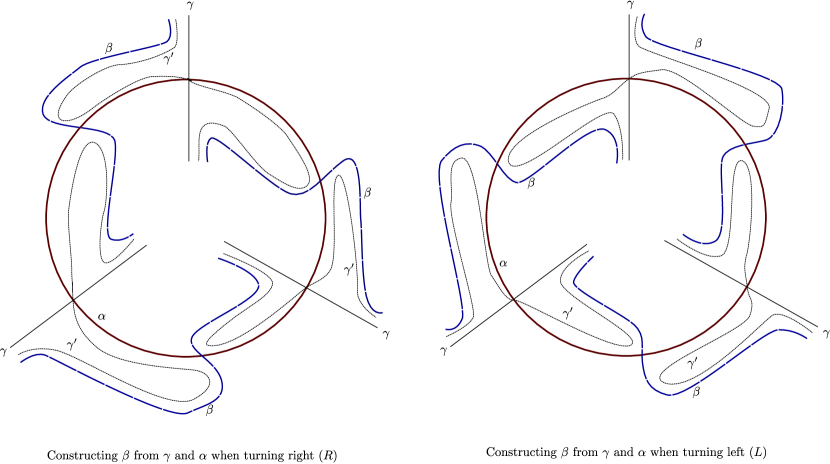
Figure 10. Constructing $\beta$

∎

Corollary 4.2.

There exists a cycle of length $2$ in the graph of multi-graftings.

Proof.

Two symmetric applications of Lemma 4.1 produces curves $\beta_{1}$ and $\beta_{2}$ so that $\mathrm{Gr}_{\gamma}=\mathrm{Gr}(\mathrm{Gr}_{\alpha},\beta_{1})$ and $\mathrm{Gr}_{\alpha}=\mathrm{Gr}(\mathrm{Gr}_{\gamma},\beta_{2})$, proving the existence of oriented cylces of length two.∎

We are now in a position to prove Theorem 1.1. Let $(S_{i},\sigma_{i})$, $i=1,2$, be projective structures with holonomy $\rho$, both different from the uniformizing structure $\sigma_{u}$. We denote by $\alpha_{1}$ and $\alpha_{2}$ the two multi-curves coding the negative annuli of $\sigma_{1}$ and $\sigma_{2}$ (that we think as a multi-geodesic with multiplicities) so that $\sigma_{i}=\text{Gr}_{\alpha_{i}}$. Consider a simple closed geodesic $\gamma$ cutting all components of $\alpha_{1}$ and all components of $\alpha_{2}$, and denote $(S_{3},\sigma_{3})=\mathrm{Gr}_{\gamma}$. By two applications of Proposition 3.3 and Lemma 4.1, there exist a multi-curve $\hat{\beta_{1}}\subset S_{1}$ and a multi-curve $\hat{\beta_{2}}\subset S_{3}$ such that $\mathrm{Gr}(\sigma_{1},\hat{\beta_{1}})=\sigma_{3}$ and $\mathrm{Gr}(\sigma_{3},\hat{\beta_{2}})=\sigma_{2}$. This proves the theorem.∎

References

- [1] Shinpei Baba. 2p-graftings and complex projective structures I. arXiv:1011.5051
- [2] Gabriel Calsamiglia, Bertrand Deroin, Stefano Francaviglia. Branched projective structures with Fuchsian holonomy. arXiv:1203.6038. To appear on Geometry & Topology.
- [3] Daniel Gallo, Michael Kapovich, and Albert Marden. The monodromy groups of Schwarzian equations on closed Riemann surfaces. Ann. of Math. (2), 151(2):625–704, 2000.
- [4] William M. Goldman. Projective structures with Fuchsian holonomy. J. Differential Geom., 25(3):297–326, 1987.
- [5] D. Hejhal. Monodromy groups and linearly polymorphic functions. Acta Math. 135 (1975) 1-55.
- [6] Kentaro Ito. Exotic projective structures and quasi-Fuchsian space. II Duke Math. J., 140(1):85–109, 2007
- [7] Feng Luo. Some applications of a multiplicative structure on simple loops in surfaces. In Knots, braids, and mapping class groups—papers dedicated to Joan S. Birman (New York, 1998), 123–129, AMS/IP Stud. Adv. Math., 24, Amer. Math. Soc., Providence, RI, 2001.
- [8] Joshua J. Thompson. Grafting Real Complex Projective Structures with Fuchsian Holonomy arXiv:1012.2194