Magnetothermal Transport in Spin-Ladder Systems

Abstract

We study a theoretical model for the magnetothermal conductivity of a spin-$\frac{1}{2}$ ladder with low exchange coupling ($J\ll\Theta_{D}$) subject to a strong magnetic field $B$. Our theory for the thermal transport accounts for the contribution of spinons coupled to lattice phonon modes in the one-dimensional lattice. We employ a mapping of the ladder Hamiltonian onto an XXZ spin-chain in a weaker effective field $B_{eff}=B-B_{0}$, where $B_{0}=\frac{B_{c1}+B_{c2}}{2}$ corresponds to half-filling of the spinon band. This provides a low-energy theory for the spinon excitations and their coupling to the phonons. The coupling of acoustic longitudinal phonons to spinons gives rise to hybridization of spinons and phonons, and provides an enhanced $B$-dependant scattering of phonons on spinons. Using a memory matrix approach, we show that the interplay between several scattering mechanisms, namely: umklapp, disorder and phonon-spinon collisions, dominates the relaxation of heat current. This yields magnetothermal effects that are qualitatively consistent with the thermal conductivity measurements in the spin-$\frac{1}{2}$ ladder compound ${\rm Br_{4}(C_{5}H_{12}N)_{2}}$ (BPCB).

I Introduction and Principal Results

Quasi one dimensional (1D) magnetic systems are present in a variety of new compounds with magnetic elements, and provide interesting manifestations of strongly correlated physics in electronic systemsgia . These systems are realized in crystals with a chain-like structure of the magnetic atoms, where intrachain exchange interactions are much stronger than interchain interactions. Their low dimensionality leads to the enhancement of quantum fluctuations, and the formation of exotic phases at low temperatures.

In particular, spin-$\frac{1}{2}$ chain systems (most commonly realized in Cu-based compounds)zotos are typically insulators in which the charge degree of freedom is frozen, and the dynamics is restricted to the spin sector. The elementary excitations are spin flips propagating along the chains direction. These can be described in terms of interacting Fermionic degrees of freedom, called spinons, which carry spin but no charge affleck . These systems therefore provide one of the simplest realizations of Luttinger liquids (LL). This spinon LL is, in fact, the most abundant form of the so-called ”spin-liquid” state, characterized by a magnetically disordered ground-state and power law spin-spin correlationsbalents-2010 .

The most elementary model for 1D spin systems is the XXZ Hamiltonianbethe , describing a spin-$\frac{1}{2}$ chain with nearest neighbor interactions,

$$H_{XXZ}=\sum_{i}J_{xy}(S_{i+1}^{x}S_{i}^{x}+S_{i+1}^{y}S_{i}^{y})+J_{z}\sum_{i}S_{i+1}^{z}S_{i}^{z}-B\sum_{i}S_{i}^{z}\;.$$ (1)

Here $J_{\alpha}>0$ corresponds to antiferromagnetic exchange interaction, and $B$ is an external magnetic field (note that here and throughout this paper we adopt units where $g\mu_{\rm B}=k_{\rm B}=\hbar=1$). The isotropic case $J_{xy}=J_{z}$ yields the 1D Heisenberg model. On each site the spin operator is represented by ${\bf S}_{i}=\frac{{\bf\sigma}_{i}}{2}$ where $\sigma^{\alpha}$ are the pauli matrices. The spin chain can be mapped into interacting spinless Fermions on a latticegia ; zotos , where the magnetic field $B$ serves as a chemical potential. At zero field the Fermions are at half filling, and upon raising the magnetic field they gradually polarize until saturation at $B=B_{c}$ which corresponds to a depletion of the spinon band.

More complicated variants of the XXZ and Heisenberg model can describe quasi 1D systems with additional interactions such as zig-zag chains, spin-Peierls chains, and laddersgia ; shelton ; dagotto . These systems support a richer phase diagram including, e.g, gapped dimer crystal phases. Upon tuning the magnetic field the system may undergo a phase transition from a gapped phase into a spin-liquidladders . In particular, in a ladder subject to a strong field $B_{c1}<B<B_{c2}$, a LL phase of gapless spinons is recoveredorig .

One of the prominent manifestations of a spin-liquid state is the contribution of gapless spinons to transport. Since there is no straightforward way to measure the spin current through an antiferromagnetic chain, investigation of the spinons properties can be done by measuring the thermal conductivity $\kappa$. Experimental evidence for a substantial enhancement of thermal conductivity along the chains direction ($\kappa_{\parallel}$), has indeed been found in CuO based chain compounds spin-ex1 ; spin-ex2 ; spin-ex3 . However, interpretation of the data is complicated by the dominant contribution of crystal phonons, and in particular their coupling to the spinons shimsh ; rozhkov . In principle, an obvious means of disentangling the spin degrees of freedom is the application of an external magnetic field $B$, which allows the tuning of system parameters in the spin sector only. The resulting magnetothermal effects – namely, variations of $\kappa$ as a function of $B$ – can serve as a valuable probe of the spin system. At low temperatures both spinons and phonons contribute to the heat transport. The total heat conductivity can be split into a pure phononic contribution, $\kappa_{ph}(T)$, and a magnetic part, $\kappa_{mag}(B,T)$. Then, we can extract the magnetothermal conductivity:

$$\Delta\kappa(B,T)=\kappa(B,T)-\kappa(0,T)=\kappa_{mag}(B,T)-\kappa_{mag}(0,T)\;.$$ (2)

Magnetothermal effects as mentioned above are practically inaccessible in the typical CuO compounds, where the large exchange coupling ($J$ of order $2000\;K$) dictates an enormous scale of the desired external field. In contrast, a field–tuned manipulation is easily accessible in organic based magnetic compounds, where $J$ is typically of order $10K$. An experiment in the organic spin-chain material ${\rm Cu(C_{4}H_{4}N_{2})(NO_{3})_{2}}$ solog1 measured the magnetothermal conductivity. It indicated a non-monotonic $B$-dependence of $\kappa_{\parallel}$, and in particular - a pronounced dip feature with a minimum at a field scale $B_{min}\sim T$. A subsequent theoretical study solog2 has shown that such feature arises due to the interplay between disorder and umklapp scattering of the spinons: the latter process is sensitive to the field-induced tuning of the spinon Fermi-level away from the middle of the band. It thus reflects the Fermionic character of the spinons.

As opposed to the spin-chain compounds mentioned above, in spin-ladder compounds, magnetothermal effects are expected to dominate at high $B$ where the spin-gap closes up. A recent experiment BPCB measured the magnetothermal conductivity in the spin-ladder compound ${\rm Br_{4}(C_{5}H_{12}N)_{2}}$ (BPCB). An experimental studyorig of thermodynamic properties of this compound confirmed that it is described very well by the spin-ladder model with $J_{\parallel}=3.6K$ (the exchange along the legs of the ladder) and $\;J_{\perp}\sim 13K$ (the exchange along the rungs), and its appropriate LL representation in the gapless regime $B_{c1}<B<B_{c2}$.

Indeed, the experimental data of Ref. [BPCB, ] indicate that upon raising the magnetic field, the magnetothermal conductivity $\Delta\kappa(B)$ vanishes for fields smaller than $B_{c1}$. However, when the magnetic field is raised further and the spin-gap is closed, there is a large decrease in the magnetothermal conductivity. On top of this decrease there is a double dip feature with a local maximum at $B_{0}=\frac{B_{c1}+B_{c2}}{2}$, corresponding to half-filling for the Fermionic excitations. We assert that this data can be qualitatively explained as follows: first, the spinons in this system are slower than the phonons, therefore they act as impurities for the phonons Rasch_thesis . This effect induces a decrease in the conductivity upon entering the spin-liquid regime ($B_{c1}<B<B_{c2}$). Second, around half-filling ($B=B_{0}$) there is a positive spinonic contribution to transport observed as a maximum at $B=B_{0}$ . The double dip feature resembles results obtained for spin-chainssolog1 ; solog2 where the minimum in the magnetothermal conductivity corresponds to moving the chemical potential away from half filling, to a scale of order $T$.

Motivated by these observations, in the present paper we study a minimal model for the magnetothermal transport of a coupled spinon-phonon system in a single ladder. Our theory accounts for a crucial distinction between ladders and chains: the strong magnetic field required to enter the gapless spinons phase provokes an enhanced coupling between spinons and phonons. This leads to hybridization between the spinons and phonons excitations. In addition, scattering of the phonons by the slower spinons is magnified, generating a relatively strong negative contribution to $\Delta\kappa(B)$. Qualitatively, our calculated $\Delta\kappa(B,T)$ resembles the experimental data of Ref. [BPCB, ].

The paper is organized as follows: in Sec. II we derive the low-energy model for the spin system in the presence of coupling to 1D phonons. In Sec. III we study the effect of scattering processes on the thermal conductivity in the framework of the memory matrix approach for the calculation of the conductivity tensor, and obtain the leading magnetic field and temperature dependencies of the thermal conductivity $\kappa$. In Sec. IV we summarize and discuss the results. Finally, in appendices A through C we present details of the calculation of the various memory matrix elements.

II Low-energy Model for the coupled spin-phonon system

We wish to compute the thermal conductivity of a system which consists of antiferromagnetic spin-$\frac{1}{2}$ ladders interacting with the lattice phonons. To this end, we focus on a simplified model for such a system, which considers a single ladder - i.e., both spinons and phonons are one-dimensional. The parameters of the model are adjusted to mimic those of BPCB BPCB , in particular assuming the limit $J_{\perp}>J_{\parallel}$ (strong rung coupling). In addition, we assume $J_{\parallel}\ll\Theta_{D}$. In this section we describe the low energy model of the system, and derive the eigenmodes which constitute the elementary excitations of the coupled spin-phonon system.

II.1 Bosonization of the spin ladder Hamiltonian

We begin by describing the spin system. The Hamiltonian of a spin-$\frac{1}{2}$ two leg ladder in a magnetic field $B$ along the $z$-direction is

$$H_{s}=\sum_{i=1}^{N}\sum_{\nu=1}^{2}[J_{\parallel}{\bf S}_{i,\nu}\cdot{\bf S}_{i+1,\nu}-BS_{i,\nu}^{z}]+\sum_{i=1}^{N}J_{\perp}{\bf S}_{i,1}\cdot{\bf S}_{i,2}\;,$$ (3)

where $\nu=1,2$ denotes the leg index. For $J_{\perp}>J_{\parallel}$, it can be approximately mapped into an effective spin-$\frac{1}{2}$ chain in a weaker magnetic fieldmilla $B_{eff}=B-B_{0}$:

$$H_{s}=\sum_{i=1}^{N}[J_{xy}^{eff}(\sigma_{i}^{x}\sigma_{i+1}^{x}+\sigma_{i}^{y}\sigma_{i+1}^{y})+J_{z}^{eff}\sigma_{i}^{z}\sigma_{i+1}^{z}]-\sum_{i=1}^{N}B_{eff}\sigma_{i}^{z}\;,$$ (4)

where the effective parameters are given by

$$J_{xy}^{eff}=J_{\parallel},\quad J_{z}^{eff}=J_{\parallel}/2\;,$$

$$B_{eff}=B-B_{0},\quad B_{0}\equiv J_{\perp}+J_{\parallel}/2\;.$$ (5)

The isospin operators $\sigma_{i}^{\alpha}$ describe the effective spin-$\frac{1}{2}$ dynamics characterizing the low energy sector, which at high $B$ is restricted to the singlet and lower triplet state on each rung. Hence, in distinction from the real-spin XXZ model [Eq. (1)], $\langle\sigma_{i}^{z}\rangle=0$ corresponds to a time-reversal symmetry broken state. To derive the low-energy model for the dynamics of this system we first use the Jordan-Wigner transformation,

$$\sigma_{i}^{+}\rightarrow c_{i}^{\dagger}\exp(i\pi\sum_{j=-\infty}^{i-1}c_{j}^{{\dagger}}c_{j}),\quad\sigma_{i}^{z}\rightarrow c_{i}^{{\dagger}}c_{i}-1/2$$ (6)

which maps the spin problem onto a model of interacting spinless Fermions on a lattice:

$$H_{s}=-t\sum_{i}(c_{i}^{{\dagger}}c_{i+1}+h.c)+V\sum_{i}(c_{i}^{{\dagger}}c_{i}-1/2)(c_{i+1}^{{\dagger}}c_{i+1}-1/2)\;,$$ (7)

where $t=J_{xy}^{eff}/2$ and $V=J_{z}^{eff}$. For $B_{eff}=0$ the Fermionic band is half-filled and the Fermi momentum is $k_{F}^{(0)}=\frac{\pi}{2a}$. Finite $B_{eff}$ corresponds to a chemical potential for the Fermions, which shifts the Fermi momentum into $k_{F}=k_{F}^{(0)}(1+M_{eff})$, with $M_{eff}$ an effective magnetization.

Near the middle of the band ($B_{eff}=0$), the Fermion operators can be expressed in terms of Bosonic ones related to the Fermion density fluctuations using the standard dictionary of abelian Bosonization (see, e.g., appendix D in Ref. [gia, ]). For the spin operators (in the continuum limit: $x=ia$) this yields

$$\sigma^{+}(x)=\frac{e^{-i\theta(x)}}{\sqrt{2\pi a}}[(-)^{x}+\cos(2\phi(x))]\;,$$

$$\sigma^{z}(x)=-\frac{1}{\pi}\partial_{x}\phi(x)+\frac{(-)^{x}}{\pi a}\cos(2\phi(x))\;,$$ (8)

where $\sigma^{\pm}(x)=\frac{1}{\sqrt{a}}\sigma_{i}^{\pm},\,\sigma^{z}(x)=\frac{1}{a}\sigma_{i}^{z}$ , and $a$ is the lattice constant. Substituting Eq. (II.1) into Eq. (4) we can describe the low energy properties of the spin system in terms of the Boson Hamiltonian:

$$H_{s}=H_{s}^{0}+H_{u}\;,$$

$$H_{s}^{0}=\frac{1}{2\pi}\int dx[g(\partial_{x}\phi(x))^{2}+v_{F}(\pi\Pi(x))^{2}]\;,$$ (9)

$$H_{u}=g_{u}\int dx\cos[4\phi(x)]\;,$$

where

$$v_{F}=aJ_{\parallel},\quad g=v_{F}\left(1+\frac{2}{\pi}\right),\quad g_{u}=-\frac{J_{\parallel}}{4\pi^{2}a}\;,$$ (10)

and $\Pi(x)=\frac{1}{\pi}\partial_{x}\theta(x)$ is the canonical conjugate of $\phi(x)$, obeying $[\Pi(x),\phi(x^{\prime})]=i\delta(x-x^{\prime})$. $H_{s}^{0}$ is the standard LL Hamiltonian

$$H_{LL}=\frac{u}{2\pi}\int dx\left[\frac{1}{K}(\partial_{x}\phi)^{2}+K(\pi\Pi)^{2}\right],$$ (11)

where

$$u=v_{F}\left(1+\frac{2}{\pi}\right)^{1/2}$$

has the dimensions of velocity and

$$K=\left(1+\frac{2}{\pi}\right)^{-1/2}$$

is the dimensionless Luttinger parameter. Since $K>1/2$, the umklapp term $H_{u}$ is irrelevant (i.e. flows to zero under renormalization group (RG) for $T\rightarrow 0$) and hence can be neglected in the description of the low-energy thermodynamic properties. However, as we shall see in the next section, it plays an essential role in the transport.

For $B\neq B_{0}$, the finite $B_{eff}$ introduces an additional term to $H_{s}^{0}$ due to the last term in Eq. (4), which induces a finite effective magnetization. The most relevant correction is of the form

$$\frac{1}{\pi}\int dxB_{eff}\partial_{x}\phi\;,$$ (12)

which can be absorbed in the Gaussian part by a shift of the field $\phi$, reflecting the shift of chemical potential for spinons. As implied by the exact Bethe ansatz solution, the LL form of $H_{s}^{0}$ is in any case maintained for arbitrarily large $B_{eff}$, but with renormalized parametersgia ; haldane . In particular $K(B_{eff})$ approaches $1$ close to the edges of the band ($B\rightarrow B_{c1}$ or $B\rightarrow B_{c2}$).

An additional correction to $H_{s}$ arises from weak disorder in the lattice, which can be accounted for by adding a random term $\delta B(x)$ to $B_{eff}$ in Eq. (4). Such term may arise from defects leading to random corrections to $J_{\perp}$, $J_{\parallel}$ via $B_{0}$ [Eq. (II.1)]. This introduces a scattering term proportional to

$$\int dx\delta B(x)\cos[2\phi(x)]\;.$$ (13)

When we discuss the relaxation of the heat current, both the umklapp and disorder terms will become important, and will be considered as perturbations of $H_{s}^{0}$.

II.2 Coupling to Lattice Phonon Modes

Up to now we described only the spin system. Next we will include the phonons in the model. In a single two-leg ladder of atoms, three modes of 1D phonons should be accounted for: two acoustic modes, longitudinal and transverse, and an optical mode associated with fluctuations in the rung length. The dominant coupling of phonons to spinons arises from the dynamical corrections to the exchange interaction, $J$, due to lattice vibrations. The spinons therefore couple to leading order only to the longitudinal acoustic mode (via fluctuations in $J_{\parallel}$) and to the optical mode (via fluctuations in $J_{\perp}$).

We first consider the effect of coupling of optical transverse phonon modes to the spinons. We show that such coupling merely leads to normalization of the Luttinger parameters, $u$ and $K$ of Eq. (11).

Let us define the transverse phonon field in the following way:

$$U_{t}(x)=U_{1}(x)-U_{2}(x),$$ (14)

where $U_{1,2}$ are transverse displacements (along the rung direction) of atoms in different legs of a ladder normalized by the rung size $b$. Now, we substitute this definition of $U_{t}$ in the phonon-dependant exchange to obtain:

$$J_{\perp}(U_{t})\approx J_{\perp}^{(0)}+\delta J_{\perp}U_{t}\;,\quad\delta J_{\perp}\equiv\left.b\frac{\partial J_{\perp}}{\partial r}\right|_{r=b}\;,$$

$$r=b(1+U_{t}).$$ (15)

Inserting into Eqs. (II.1) and (12), we find that this adds to the Hamiltonian a term of the form

$$H_{sp}^{t}=-\delta J_{\perp}\int\frac{dx}{2\pi}U_{t}(x)\partial_{x}\phi(x).$$ (16)

It is useful to change into momentum representation with

$$U_{t}(x)=\sqrt{\frac{a}{L}}\sum_{k}(b_{k}e^{ikx}+b_{k}^{\dagger}e^{-ikx}),\quad\phi(x)=\sqrt{\frac{a}{L}}\sum_{k}(\phi_{k}e^{ikx}+\phi_{-k}e^{-ikx})$$ (17)

(where $L$ is the length of the legs). Then, the quadratic part of the coupled spinon-phonon Hamiltonian is given by

$$H=H_{s}^{0}+H_{p}^{t}+H_{sp}^{t},$$ (18)

where $H_{s}^{0}$ describes the spinons in terms of a Luttinger Hamiltonian [Eq. (11)],

$$H_{p}^{t}=\omega_{0}\sum_{k}b_{k}^{{\dagger}}b_{k}$$ (19)

describes the optical transverse phonons, and

$$H_{sp}^{t}=-\delta J_{\perp}a\sum_{k}ik(\phi_{k}b_{k}^{{\dagger}}-\phi_{-k}b_{k})$$ (20)

is the spinon-phonon interaction. Using a coherent path integral representation, it is a straightforward exercise to integrate over the phonon degrees of freedom, yield an effective action for the spinons, $S_{eff}$, defined as

$$e^{-S_{eff}[\phi]}=\int D\overline{b}Dbe^{-S[\phi,\overline{b},b]}.$$

In the limit $k,\;\omega_{n}\rightarrow 0$ this results in a Luttinger model with a modified coefficient of $(\partial_{x}\phi)^{2}$:

$$\frac{u}{K}\rightarrow\frac{u}{K}+\frac{\delta J_{\perp}^{2}a}{\omega_{0}}.$$ (21)

Hence, the renormalized parameters become:

$$\tilde{K}=K\left[1+\frac{\delta J_{\perp}^{2}aK}{\omega_{0}u}\right]^{-1/2},\quad\tilde{u}=u\left[1+\frac{\delta J_{\perp}^{2}aK}{\omega_{0}u}\right]^{1/2}.$$ (22)

Next we focus on the longitudinal phonons, which coupling to the spin sector has the most dramatic consequences. Assuming small displacements of atoms from their equilibrium positions, we can approximate the exchange interaction by:

$$J_{\parallel}(r)\approx J_{\parallel}^{(0)}+g_{\parallel}\partial_{x}U_{l}(x),\quad g_{\parallel}\equiv a^{2}\frac{\partial J_{\parallel}}{\partial r}|_{r=a},$$ (23)

where $r=a[1+U_{l}(x+a)-U_{l}(x)]$ is the distance between neighboring atoms on the same leg, and the dimensionless field $U_{l}(x)$ describes the relative longitudinal displacements of atoms. When inserted into Eq. (4), these corrections give rise to coupling between the spinons and phonons. The Hamiltonian describing longitudinal phonons traveling parallel to the chains is

$$H_{p}^{l}=\frac{v}{2\pi}\int dx[(\pi P_{l}(x))^{2}+(\partial_{x}U_{l}(x))^{2}],$$ (24)

where $v\sim a\Theta_{D}$ (with $\Theta_{D}$ the Debye temperature) is the sound velocity, and $P_{l}$ is the momentum conjugate to $U_{l}$.

After inserting the phonon-dependant correction to the exchange interaction into Eqs. (II.1), (II.1) and (12), and adding the phonon Hamiltonian [Eq. (24)], the low-energy Hamiltonian of the coupled spin-phonon system can be written as:

$$H_{0}=\frac{1}{2\pi}\int dx\left\{g(\partial_{x}\tilde{\phi}(x))^{2}+v_{F}(\pi\Pi(x))^{2}+h_{l}\partial_{x}U_{l}(x)\partial_{x}\tilde{\phi}(x)\right.$$

$$\left.+v[(\partial_{x}U_{l}(x))^{2}+(\pi P_{l}(x))^{2}]+\frac{g_{\parallel}B_{eff}^{(0)}}{g}\partial_{x}U_{l}(x)\right\},$$ (25)

with

$$h_{l}\equiv-g_{\parallel}\left[1+\frac{2(1+2/\pi)B_{eff}^{(0)}a}{g}\right],$$

$$\partial_{x}\tilde{\phi}(x)\equiv\partial_{x}\phi(x)+\frac{B_{eff}^{(0)}}{g},\quad B_{eff}^{(0)}\equiv B-J_{\perp}^{(0)}-J_{\parallel}^{(0)}/2.$$ (26)

In Eq. (25) we neglected small terms (of order $\partial_{x}U_{l}(\partial_{x}\phi)^{2}$ and higher). These terms are irrelevant, and moreover correspond to forward scattering that cannot contribute to transport properties of the spinons to leading order. Note that, in contrast with spin-chains shimsh , at half-filling ($B_{eff}^{(0)}=0$) the coupling to the phonons via the coupling constant $h_{l}$ is linear in the spinon field $\partial_{x}\phi$ and has to be included in the low-energy Hamiltonian. This reflects the breaking of time-reversal symmetry in the system, where spinons correspond to fluctuations around a partially polarized magnetic state. Below we show how these terms lead to new eigenmodes of mixed spinon-phonon degrees of freedom.

II.3 Derivation of Hybrid Eigenmodes

The Hamiltonian $H_{0}$ in Eq. (25) describes the low energy properties of the coupled spinon-phonon system. In order to find the eigenmodes which constitute the elementary degrees of freedom of the system, we proceed in diagonalizing it by a canonical transformationshimsh :

$$\tilde{\phi}(x)=C\phi_{1}(x)-\lambda^{2}S\phi_{2}(x),$$

$$U_{l}(x)=\frac{1}{\lambda^{2}}S\phi_{1}(x)+C\phi_{2}(x),$$ (27)

and similarly for the canonically conjugate momentum:

$$\Pi(x)=C\Pi_{1}(x)-\frac{1}{\lambda^{2}}S\Pi_{2}(x),$$

$$P_{l}(x)=\lambda^{2}S\Pi_{1}(x)+C\Pi_{2}(x),$$ (28)

where:

$$C\equiv\frac{1}{\sqrt{2}}\left[1-\frac{1}{\sqrt{A^{2}+1}}\right]^{1/2},\quad S\equiv\frac{1}{\sqrt{2}}\left[1+\frac{1}{\sqrt{A^{2}+1}}\right]^{1/2},$$

$$\lambda^{2}\equiv\sqrt{v_{F}/v},\quad A\equiv\frac{h_{l}\sqrt{v_{F}/v}}{gv_{F}/v-v}\approx-\frac{h_{l}}{v}\sqrt{\frac{v_{F}}{v}}\ll 1.$$ (29)

Eqs. (II.3) and (II.3) are designed to preserve the canonical commutation relations $[\phi_{\nu}(x),\Pi_{\nu^{\prime}}(x^{\prime})]=i\delta_{\nu\nu^{\prime}}\delta(x-x^{\prime})$. The last approximation in Eq. (II.3) assumes $v_{F}\ll v$, which follows from $J_{\parallel}\ll\Theta_{D}$. The parameter $A$ defines the strength of the coupling between the spinons and phonons. Note that it would be much stronger in a compound where $J\sim\Theta_{D}$, in which case the phonon and spinon velocities match, $v_{F}\sim v$.

After this transformation, $H_{0}$ [Eq. (25)] takes the form

$$H_{0}=\frac{1}{2\pi}\int dx\left\{\sum_{\nu=1,2}\left[\frac{v_{\nu}}{K_{\nu}}(\partial_{x}\phi_{\nu}(x))^{2}+v_{\nu}K_{\nu}(\pi\Pi_{\nu}(x))^{2}\right]\right.$$

$$\left.+\frac{h_{l}B_{eff}}{g}\left[\frac{S}{\lambda^{2}}\partial_{x}\phi_{1}(x)+C\partial_{x}\phi_{2}(x)\right]\right\},$$ (30)

with

$$\frac{v_{1}}{K_{1}}=\frac{1}{2\sqrt{A^{2}+1}}\left[g(\sqrt{1+A^{2}}-1)+\frac{v^{2}}{v_{F}}(\sqrt{1+A^{2}}+1)+\sqrt{\frac{v}{v_{F}}}h_{l}A\right],\quad v_{1}K_{1}=v_{F}$$

$$\frac{v_{2}}{K_{2}}=\frac{1}{2\sqrt{A^{2}+1}}\left[\frac{gv_{F}}{v}(\sqrt{1+A^{2}}+1)+v(\sqrt{1+A^{2}}-1)-h_{l}\sqrt{\frac{v_{F}}{v}}A\right],\quad v_{2}K_{2}=v,$$

which can be approximated for $v_{F}\ll v$ by

$$\frac{v_{1}}{K_{1}}\approx\frac{v^{2}}{v_{F}}\left(1-\frac{3A^{2}}{4}\right),\quad\frac{v_{2}}{K_{2}}\approx\frac{gv_{F}}{v}\left(1+\frac{3A^{2}v^{2}}{4gv_{F}}\right).$$ (32)

In this form, $H_{0}$ is separable into two independent species of LLs. Using $A\ll 1$, the LL parameters are approximated by

$$v_{1}\approx v\left(1-\frac{3A^{2}}{4}\right)^{1/2}\;,\quad v_{2}\approx v_{F}\sqrt{\left(1+\frac{2}{\pi}\right)\left(1+\frac{3A^{2}v^{2}}{4gv_{F}}\right)},$$

$$K_{1}\approx\frac{v_{F}}{v}\left(1+\frac{3A^{2}}{4}\right)^{1/2},\quad K_{2}\approx\frac{v}{v_{F}}\sqrt{\frac{1+\frac{3A^{2}v^{2}}{4gv_{F}}}{1+\frac{2}{\pi}}}.$$ (33)

Finally, to get rid of the linear terms $\partial_{x}\phi_{1}(x)$ and $\partial_{x}\phi_{2}(x)$ in Eq. (30), we define

$$\tilde{\phi}_{1}(x)=\phi_{1}(x)+\frac{B_{eff}K_{1}h_{l}S}{2v_{1}g\lambda^{2}}x\;,$$

$$\tilde{\phi}_{2}(x)=\phi_{2}(x)-\frac{B_{eff}K_{2}h_{l}C}{2v_{2}g}x\;,$$ (34)

and

$$\tilde{\Pi}_{1}(x)=\Pi_{1}(x),\quad\tilde{\Pi}_{2}(x)=\Pi_{2}(x)$$ (35)

which preserve the canonical commutation relations. The low energy Hamiltonian is now cast in the quadratic form of a LL:

$$H_{0}=\sum_{\nu=1}^{2}v_{\nu}\int\frac{dx}{2\pi}\left[\frac{1}{K_{\nu}}(\partial_{x}\tilde{\phi}_{\nu}(x))^{2}+K_{\nu}(\pi\tilde{\Pi}_{\nu}(x))^{2}\right].$$ (36)

The Hamiltonian (36) is integrable (i.e. it has an infinite number of conservation laws), therefore the currents we are interested in (e.g heat current) are protected and cannot degrade. In order to get a finite conductivity we must add perturbations around $H_{0}$, e.g. the previously neglected umklapp term, which in terms of the shifted spinon field is given by

$$H_{u}=g_{u}\int dx\cos[4\tilde{\phi}(x)-\Delta kx],\;\Delta k\equiv\frac{4B_{eff}}{g}.$$ (37)

$H_{u}$ describes processes where two spinons move from the right Fermi surface to the left (or vice versa), gathering momentum $\Delta k=4k_{F}-G$ in which $G=\frac{2\pi}{a}$ is the reciprocal lattice momentum. Another important correction to $H_{0}$ is the backscattering term

$$H_{d}=\int dx\zeta(x)\cos[2\tilde{\phi}(x)],\;\zeta(x)\equiv\frac{\delta B(x)}{\pi a}\;,$$ (38)

which describes scattering of spinons due to weak disorder caused by defects in the lattice. We assume uncorrelated random disorder where the sample average gives

$$\overline{\zeta(x)}=0,$$

$$\overline{\zeta(x)\zeta(x^{\prime})}=D\delta(x-x^{\prime})\;.$$ (39)

Using Eq. (II.3), $H_{u}$ and $H_{d}$ can be expressed in terms of the hybrid spinon-phonon eigenmodes $\phi_{1}(x)$, $\phi_{2}(x)$:

$$H_{u}=g_{u}\int dx\cos(2\alpha\phi_{1}(x)-2\beta\phi_{2}(x)-\Delta kx),$$

$$H_{d}=\int dx\zeta(x)\cos(\alpha\phi_{1}(x)-\beta\phi_{2}(x)),$$ (40)

with

$$\alpha\equiv 2C,\quad\beta\equiv 2\lambda^{2}S\;.$$ (41)

Finally, we note that higher orders in the expansions Eq. (15) and (23) yield an additional scattering term between phonons and spinons, which turns out to have a significant effect on the transport carried by phonons. subsection III.2 is devoted to a detailed study of the implication of this term on the thermal conductivity. Together with $H_{d},\;H_{u}$ [Eqs. (37) and (38)], this scattering process governs the degrading of currents leading to a finite conductivity.

III Thermal Transport of the Spin-Ladder System

The magnetothermal effects observed, e.g., in Ref. [BPCB, ] are a consequence of the interplay between different scattering mechanisms which result in the change of the thermal conductivity as a function of magnetic field $[\kappa(B)]$. Two primary effects are expected to dominate the $B$-dependance in the coupled phonon-spinon system: one arises from the positive contribution of spinons as heat carriers, and the other from the negative contribution of spinons acting as scatterers of the phonons. The former contribution is governed by the interplay of two scattering mechanisms, umklapp and disorder, and consequently depends on the deviation of the spinon chemical potential from a commensurate valuesolog2 . At the same time, the scattering due to phonon-spinon interaction is also dependant on the filling of the spinon band, which dictates the available phase-space for scattering. We note that due to the hybridization of phonons and spinons, these various effects are not entirely separable. In the present section we derive the magnetothermal conductivity of the spin-ladder model by using a memory matrix formalism, which allows an account of all the above mentioned scattering processes on equal footing.

III.1 Approximate Conservation Laws and Memory Matrix Formalism

To calculate the heat conductivity of the spin-ladder system, we use the memory matrix formalism forster which has been successfully implemented in previous studies of thermal transport in spin-chainsshimsh ; solog2 . The memory-matrix approach is suited for systems where due to approximate conservation laws, the conductivity almost diverges AR . The main step within this approach is the calculation of a matrix of relaxation rates for a given set of slow modes. The method allows to calculate transport coefficients within a hydrodynamic approximation, and provides a reliable lower bound to the conductivity Jung . Moreover, it gives precise results as long as all the relevant slow modes are included in the calculation.

The heat transport properties of the spin–ladder system at low temperature are governed by the approximate conservation of a certain current, $J_{c}$ which has a finite overlap with the heat current. In particular, an exponentially slow decay of $J_{c}$ will lead to an exponentially large heat conductivity: the component of the heat current overlapping with $J_{c}$ is protected, and will decay exponentially slowly.

In the present case, the important step is to realize that in the absence of disorder, the linear combination

$$J_{c}=J_{\phi}-\frac{\Delta k}{4}J_{s}$$ (42)

is conserved, meaning $[J_{c},H_{0}+H_{u}]=0$, where $H_{0}$ is the LL Hamiltonian (36), and $H_{u}$ the umklapp term [Eq. (37)]. Here,

$$J_{\phi}=\int dx\Pi(x)\partial_{x}\phi(x),$$

$$J_{s}=N_{R}-N_{L}=\int dx\Pi(x),$$ (43)

are the (normalized) heat current associated with the spinons and the spin current, respectively, where $N_{R}$ and $N_{L}$ are the total number of right or left moving spinons. The overlap between the heat current and the conserved current is manifested by the appearance of $J_{\phi}$ in Eq. (42). The reason that $J_{c}$ is conserved by umklapp scattering is as follows: the umklapp term describes a process where a momentum $\Delta k$ is generated and therefore induces a change in $J_{\phi}$ proportional to $\Delta k$. In the same process, the normalized spin current is changed by $-4$ as two right-moving spinons are scattered into left-moving states. Since $J_{c}$ is conserved by the umklapp term $H_{u}$, the heat current can not be degraded by $H_{u}$ alone and additional scattering processes need to be accounted for.

The low-energy Hamiltonian $H_{0}$ conserves an infinite number of modes in addition to $J_{c}$. However, when perturbations are added, these modes decay faster than the conserved current $J_{c}$, since these modes do not commute with all the terms added.

We now show how to calculate perturbatively the thermal conductivity when the relaxation of the heat current is dominated by the slow modes. In our case the memory matrix is formulated in a space spanned by the slow modes $J_{1}$, $J_{2},\;J_{3}$ and $J_{s}$ [Eq. (III.1)], where

$$J_{1}=\int dx\Pi_{1}(x)\partial_{x}\phi_{1}(x), J_{2}=\int dx\Pi_{2}(x)\partial_{x}\phi_{2}(x),$$

$$J_{3}=\int dx\Pi_{3}(x)\partial_{x}\phi_{3}(x)$$ (44)

which are all conserved by $H_{0}$. The fields $\phi_{3},\Pi_{3}$ represent the transverse acoustic phonons which do not hybridize with spinons but are still scattered by spinons and therefore contribute to relaxation of the heat current. The heat current along the chains direction is $J_{Q}=v_{1}^{2}J_{1}+v_{2}^{2}J_{2}+v_{3}^{2}J_{3}$, where $v_{1}$ and $v_{2}$ are given in Eq. (33).

To set up the memory matrix formalismforster , we first introduce a scalar product on the operators in the space spanned by the slow modes

$$(A(t)|B)=T\int_{0}^{1/T}d\lambda\langle A^{\dagger}(t)B(i\lambda)\rangle,$$ (45)

where $\langle...\rangle$ denotes an expectation value at equilibrium, including average over disorder configurations. The dynamic correlation function of the operators A and B is

$$\chi_{AB}(\omega)=\int_{0}^{\infty}dte^{i\omega t}(A(t)|B)$$

$$=\frac{iT}{\omega}\int_{0}^{\infty}dte^{i\omega t}<[A(t),B]>-\frac{(A|B)}{i\omega},$$ (46)

and the matrix of conductivities is given by

$$\sigma_{pq}(\omega)=\frac{1}{TL}\chi_{J_{p}J_{q}}(\omega)$$ (47)

where $p,q$ are either of the slow modes. The heat conductivity is given by

$$\kappa=\frac{1}{T}\sigma_{QQ}$$ (48)

where $J_{Q}$ denotes the heat current. One can also write the matrix of static susceptibilities as

$$\chi_{pq}=\frac{1}{TL}(J_{p}|J_{q})\;.$$ (49)

It can be shown forster that the matrix of conductivities, $\hat{\sigma}$, can be expressed in terms of a memory matrix, $\hat{M}$

$$\hat{\sigma}=\hat{\chi}(T)[\hat{M}(\omega,T)-i\omega\hat{\chi}(T)]^{-1}\hat{\chi}(T)\;.$$ (50)

The elements of the matrix $\hat{M}(\omega)$ in the d.c. limit ($\omega\rightarrow 0$) are

$$M_{pq}=\lim_{\omega\to 0}\frac{C_{pq}(\omega)-C_{pq}(\omega=0)}{i\omega}\rightarrow-i\partial_{\omega}C_{pq}|_{\omega=0}$$ (51)

where $p,\;q$ can be each of the slow modes of the theory, and $C_{pq}(\omega)$ is the Fourier transform of the retarded correlation function,

$$C_{pq}(\omega)=\int_{0}^{\infty}dte^{i\omega t}\langle[F_{p}(t),F_{q}(0)]\rangle,$$ (52)

of the force operators:

$$F_{p}\sim\dot{J}_{p}=i[H,J_{p}]=i[H^{pert},J_{p}].$$ (53)

Here $H^{pert}$ stands for perturbations to the low-energy Hamiltonian of the system $H_{0}$, that can relax the current $J_{p}$ [such as $H_{u}$, $H_{d}$, Eqs. (37), (38)]. In the last equality we used $[J_{p},H_{0}]=0$ for $p=s,1,2,3$, which justifies a perturbative expansion of $\hat{M}$: since $\dot{J}_{p}$ are already linear in perturbations around $H_{0}$, the expectation values in Eq. (49) and (52) are computed with respect to $H_{0}$.

From Eqs. (48) and (50) it follows that the d.c. thermal conductivity is given by

$$\kappa=\frac{1}{T}\hat{\chi}\hat{M}^{-1}\hat{\chi}\;.$$ (54)

The static susceptibility matrix is given by

$$\hat{\chi}=\left({\begin{array}[]{*{20}c}\frac{2}{\pi v_{F}}&0&0&0\\ 0&\frac{\pi T^{2}}{3v_{1}^{3}}&0&0\\ 0&0&\frac{\pi T^{2}}{3v_{2}^{3}}&0\\ 0&0&0&\frac{\pi T^{2}}{3v_{3}^{3}}\end{array}}\right)$$ (59)

(where the matrix indices are $s,1,2,3$). In our case the three leading perturbations contributing to the memory matrix, $\hat{M}$, are umklapp and disorder in the spin sector, and phonon scattering processes which include phonon-spinon interaction. Thus, the memory matrix is separated into three parts,

$$\hat{M}=\hat{M}^{u}+\hat{M}^{d}+\hat{M}^{p-s}\;.$$ (60)

Using the conservation law of the slow mode $J_{c}$ [Eq. (42)] we find relations between the different umklapp matrix elements (see appendix A):

$$M_{s1}^{u}=\frac{\Delta k}{4}M^{u}_{ss}-M_{s2}^{u},$$

$$M_{12}^{u}=\frac{\Delta k}{4}M_{s2}^{u}-M_{22}^{u},$$ (61)

$$M_{11}^{u}=\frac{\Delta k}{4}M_{s1}^{u}-M_{12}^{u}.$$

When $v_{F}\ll v$, and thus $K_{1}\alpha^{2}\ll K_{2}\beta^{2}$ [see Eq. (41)], the matrix $\hat{M}^{u}$ greatly simplifies. Using the relations (III.1) we find that the leading contribution to $\hat{M}^{u}$ depends only on one element $M_{ss}^{u}=M_{s}^{u}$, and we have

$$\hat{M}^{u}\cong\left({\begin{array}[]{*{20}c}M_{s}^{u}&0&\frac{\Delta k}{4}M_{s}^{u}&0\\ 0&0&0&0\\ \frac{\Delta k}{4}M_{s}^{u}&0&(\frac{\Delta k}{4})^{2}M_{s}^{u}&0\\ 0&0&0&0\end{array}}\right).$$ (66)

The disorder contribution, $\hat{M}^{d}$, is a diagonal matrix with elements denoted by $M^{d}_{pp}=M^{d}_{p}$ ($p=s,1,2,3$). Finally, the dominant contribution from phonon-phonon and phonon-spinon scattering, $\hat{M}^{p}$, appears in the diagonal elements $M_{1}$, $M_{3}$ (a detailed calculation is provided in the next subsection).

Substituting these relations into Eq. (54), we obtain an expression for the thermal conductivity

$$\kappa(B,T)\cong\frac{1}{T}\left[\frac{v_{1}^{4}\chi_{11}^{2}}{M_{1}}+\frac{16v_{2}^{4}\chi_{22}^{2}(M_{s}^{d}+M_{s}^{u})}{\Delta k^{2}M_{s}^{d}M_{s}^{u}+16M_{2}^{d}(M_{s}^{d}+M_{s}^{u})}+\frac{v_{3}^{4}\chi_{33}^{2}}{M_{3}}\right]\;.$$ (67)

The $B$-dependance of this expression is encoded in the various matrix elements $M^{u}_{s},\;M_{s}^{d}\;,M_{1}$ and $M_{3}$. We note that the scattering processes in the spin sector (described by $M_{s}^{u},\;M_{s}^{d}$) dominate near half-filling of the spinon band, where their spectrum can be linearized and Bosonization is justified. Using Eq. (II.3) for the relevant terms in the Hamiltonian, we derive $M_{s}^{u}$ (for a detailed calculation, see appendix A),

$$M_{s}^{u}=g_{s}\left(\frac{T}{T_{0}}\right)^{2K_{2}\beta^{2}+2K_{1}\alpha^{2}-3}B[K_{2}\beta^{2}/2-i\delta,1-K_{2}\beta^{2}]B[K_{2}\beta^{2}/2+i\delta,1-K_{2}\beta^{2}]\Re[\Psi(1-K_{2}\beta^{2}/2-i\delta)-(\Psi(K_{2}\beta^{2}/2+i\delta)]$$

$$g_{s}\equiv\frac{g_{u}^{2}}{2\pi^{2}}\sin(\pi K_{2}\beta^{2}),\quad\delta\equiv\frac{v_{2}\Delta k}{4\pi T},\quad T_{0}\equiv\frac{v_{2}}{2\pi a},$$ (68)

where $B(x,y)=\frac{\Gamma(x)\Gamma(y)}{\Gamma(x+y)}$ is the Beta function, $\Psi(x)=\frac{\Gamma^{\prime}(x)}{\Gamma(x)}$ is the digamma function and the parameters $K_{1},\;K_{2},\;\alpha$ and $\beta$ are defined in Eqs. (33) and (41). The dimensionless parameter $\delta$ determines the dominant field dependance of $\hat{M}^{u}$ via $\Delta k$ [see Eq. (37)]. For the disorder part of $\hat{M}$ we find

$$\hat{M}^{d}=\left({\begin{array}[]{*{20}c}D_{s}\left(\frac{T}{T_{0}}\right)^{K_{2}\beta^{2}/2+K_{1}\alpha^{2}/2-2}&0&0&0\\ 0&D_{1}\left(\frac{T}{T_{0}}\right)^{K_{2}\beta^{2}/2+K_{1}\alpha^{2}/2}&0&0\\ 0&0&D_{2}\left(\frac{T}{T_{0}}\right)^{K_{2}\beta^{2}/2+K_{1}\alpha^{2}/2}&0\\ 0&0&0&0\end{array}}\right)$$ (73)

with

$$D_{s}\cong\frac{4\pi Da^{2}}{v_{2}^{3}},\;D_{1}\cong\frac{DK_{1}\alpha^{2}}{2v_{1}},\;D_{2}\cong\frac{DK_{2}\beta^{2}}{2v_{2}}$$ (74)

where $D$ is defined in Eq. (39). The $B$-dependance of $\hat{M}^{d}$ is implicit in the parameters $K_{1},\;K_{2},\;\alpha,\;\beta$.

Incorporating Eqs. (III.1), (73) in the second term of Eq. (67), we find the primary magnetothermal effects originating from relaxation processes in the spin sector. To complete the derivation of $\kappa(B,T)$, one must account for the $B$-dependance of $M_{1}$, $M_{3}$ originating from phonon-spinon interaction. This part of the derivation requires special attention, and is discussed in subsection B below.

III.2 Phonon-Spinon Scattering

As already mentioned above, we focus on ladders with small exchange coupling obeying $J_{\parallel}\ll\Theta_{D}$, where the phonons typical velocity is much larger than the spinons velocity. Therefore, the spinons act as impurities which scatter the phonons. These scattering processes lead to relaxation of the phononic heat current and therefore to a prominent dip in the thermal conductivity upon entering the partially filled spinon band, for $B_{c1}<B<B_{c2}$. These add a $B$-dependant contribution to the scattering rate of both longitudinal and transverse branches of acoustic phonons (represented by the Bosonic fields $U_{l},\phi_{3}$). Below we study the contribution of phonon-spinon scattering processes to the corresponding memory matrix elements.

In order to account for scattering processes of phonons on spinons, we expand the phonon-dependant exchange (23) to second order in $\partial_{x}U_{l}$. The most relevant phonon scattering term arising from this order of the expansion is of the form

$$H_{p-s}=g_{p-s}\int\frac{dx}{2\pi}(\partial_{x}U_{l})^{2}\partial_{x}\phi.$$ (75)

A similar term resulting from the transverse displacements yields a coupling of spinons density to $(\partial_{x}\phi_{3})^{2}$. We wish to consider magnetic-field dependance in a wide range, i.e. the entire spinon-band. For this purpose we model the spinons as free Fermions at a chemical potential dictated by $B$, a reasonable approximation, e.g., for the ladders in BPCB where the Luttinger parameter $K$ is not far from 1 for arbitrary $B$ [orig, ]. Using $\partial_{x}\phi(x)=-\pi\rho(x)$ [gia, ], and turning to Fourier space, $H_{p-s}$ acquires the form:

$$H_{p-s}=\sum_{kk^{\prime}pp^{\prime}G_{n}}V_{pp^{\prime}}c_{k^{\prime}}^{{\dagger}}c_{k}b_{p^{\prime}}^{{\dagger}}b_{p}\delta(k-k^{\prime}+p-p^{\prime}-G_{n}),$$

$$V_{pp^{\prime}}=\frac{g_{p-s}pp^{\prime}}{\sqrt{\omega_{p}\omega_{p^{\prime}}}},$$ (76)

where $c_{k}$ is a Fermionic (spinon) annihilation operator, and $b_{p}$ is a Bosonic (phonon) annihilation operator. $H_{p-s}$ describes elastic scattering where a phonon and a spinon with momenta $p$ and $k$ respectively, scatter into $p^{\prime}$ and $k^{\prime}$ respectively.

We need to calculate the effect of this term on the phononic heat current

$$J_{ph}^{E}=\sum_{p}v_{p}\omega_{p}b_{p}^{{\dagger}}b_{p},\quad v_{p}=\frac{\partial\omega_{p}}{\partial p}\approx v\,\text{sign}(p),$$ (77)

where we have assumed a linear dispersion $\omega_{p}\approx v|p|$. The memory matrix element [Eq. (51)] is therefore calculated with the correlation function (52) of the force operator

$$F_{p-s}\sim[J_{ph}^{E},H_{p-s}].$$ (78)

Using Wick’s theorem we obtain an expression for this correlation function (see appendix C for details)

$$C_{p-s}=\sum_{kpq}W_{pq}\delta(\Delta\omega)n_{p+q}f_{k-q}(1+n_{p})(1-f_{k}),$$

$$W_{pq}=-2v^{2}g_{p-s}^{2}|p(p+q)|q^{2},\quad q\equiv p^{\prime}-p,$$

$$\Delta\omega\equiv\epsilon_{k}-\epsilon_{k-q}+\omega_{p}-\omega_{p+q},$$ (79)

where $f_{k}=(e^{(\epsilon_{k}-\mu)/T}+1)^{-1},\;n_{p}=(e^{\omega_{p}/T}-1)^{-1}$, are Fermi and Bose distributions respectively. The memory matrix element is the derivative of $C_{p-s}$ with respect to $\omega$. Integrating by parts and using the energies delta function we obtain:

$$M_{p-s}=\int dkdp\frac{\partial}{\partial q}\left[\frac{W_{pq}n_{p+q}f_{k-q}(1+n_{p})(1-f_{k})}{\frac{\partial\Delta\omega}{\partial q}}\right]_{q=q_{0}}\frac{1}{\frac{\partial\Delta\omega}{\partial q}|_{q=q_{0}}},$$ (80)

where $q_{0}$ is the momentum transfer that obeys the energy and momentum conservation dictated by the delta functions. Since the phonon dispersion $\omega_{p}=v|p|$ is much steeper than the spinon dispersion $\epsilon_{k}=-J_{\parallel}^{(0)}\cos(ka)$ , energy and momentum conservation can only be satisfied by phonon backscattering where $p\rightarrow p+q=-p+\delta p,\;|\delta p|<<|p|$. This is because a small change in phonon momentum will lead to a large energy change, while the spinon energy transfer is small for small momentum transfer (see Fig. 1).

Figure 1: (color online) Schematic Plot of the phonons (red) and the spinons (green) energy dispersions, the allowed phonon backscattering (red curved arrow) and the corresponding spinon scattering (green curved arrow). The black arrows represent the momentum transfer $q_{0}=p^{\prime}-p=k-k^{\prime}$.

The integrals in Eq. (80) were solved numerically after approximating

$$\delta p\cong\frac{J_{\parallel}^{(0)}}{v}[\cos(k+2p)-\cos(k)]\;,$$

to get the temperature and field dependencies of $M_{p-s}$ (see Figs. 2, 3). The memory matrix is closely related to the relaxation time of the scattering process $M_{p-s}\sim\tau_{p-s}^{-1}$. Indeed as indicated by Fig. 2, phonon scattering occurs practically only for $B_{c2}<B<B_{c1}$, in the spin-liquid phase where the spinons are gapless, and it is maximal for $B=B_{0}$ (half filling of the spinon band).

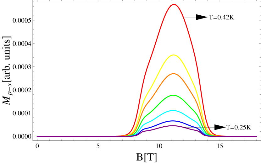
Figure 2: (color online) Isotherms of $M_{p-s}$ as a function of magnetic field for various temperatures $T=0.25K,\,0.27K,\,0.30K,\,0.33K,\,0.36K,\,0.38K,\,\,0.42K$. The parameters used for this plot: $J_{\parallel}=3.6K,\,J_{\perp}=14.4K,\,g_{p-s}=0.04$, $\frac{v}{a}=18K$.

The temperature dependance of $M_{p-s}$ (Fig. 3) for $B_{eff}=0$ gives a good fit to a power law $M_{p-s}\sim T^{\sigma}$, with $\sigma\cong 4.5$.

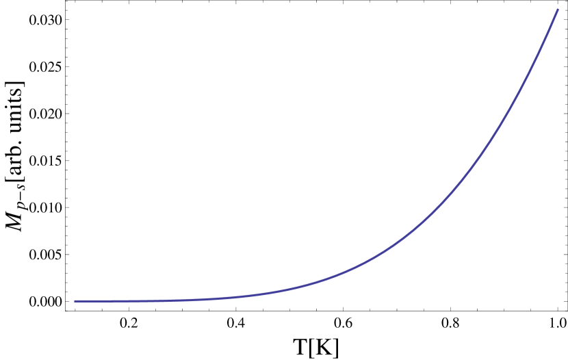
Figure 3: (color online) $M_{p-s}$ at half-filling ($B_{eff}=0$) as a function of temperature. The parameters used for this plot: $J_{\parallel}=3.6K,\,J_{\perp}=14.4K,\,g_{p-s}=0.04,\,\frac{v}{a}=18K$.

We next recall that under the approximation $v_{F}\ll v$, one obtains $\alpha\ll\beta$ [see Eqs. (II.3), (41)], which implies that one hybrid mode $\phi_{1}$ is phonon-like, while $\phi_{2}$ is spinon-like. Therefore, the scattering of longitudinal phonons is included to a good approximation only in the $M_{1}$ element of the memory matrix. This is added to the disorder term already retrieved earlier, and a $B$-independent contribution which assumes a power-law dependance on $T$. We thus obtain an expression of the form

$$M_{1}=D_{1}\left(\frac{T}{T_{0}}\right)^{K_{2}\beta^{2}/2+K_{1}\alpha^{2}/2}+D_{p}T^{\gamma}+M_{p-s}\;.$$ (81)

A similar expression, excluding the first term, holds for $M_{3}$ which describes the scattering of transverse acoustic phonons. Substituting in (67), we obtain the final expression for $\kappa(B,T)$ and consequently for $\Delta\kappa(B,T)$ [Eq. (2)]. The resulting $B$ and $T$ dependance of $\Delta\kappa(B)/\kappa(0)$ are plotted as a function of magnetic field for different temperatures (Fig. 4). We note that this result, although based on a highly simplified minimal model which captures the main physics of the system, qualitatively reproduces the prominent features of the experimental data of Ref. BPCB, .

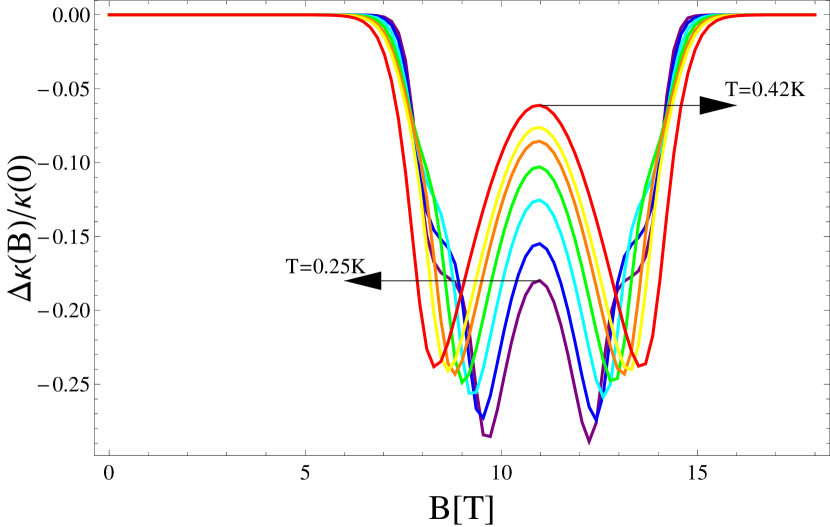
Figure 4: (color online) Isotherms of the normalized magnetothermal conductivity as a function of magnetic field for various temperatures $T=0.25K,\,0.27K,\,0.30K,\,0.33K,\,0.36K,\,0.38K,\,\,0.42K$. The parameters used for this plot: $J_{\parallel}=3.6K,\,J_{\perp}=14.4K,\,g_{p-s}=0.04,\,D=1.6\times 10^{-8},\,\,\frac{v}{a}=18K,\,D_{p}=7.4\times 10^{-8},\,D_{3}=4.6\times 10^{-6},\,\gamma=4$.

IV Summary and Discussion

In this work we studied the thermal conductivity of weakly disordered spin ladders subject to a magnetic field and coupled to phonons. We found that due to coupling between the phonons and the spins, the elementary degrees of freedom are hybrid spinon-phonon modes and strong scattering of phonons on spinons is induced. Our study of the phonon-spinon scattering found that due to energy and momentum conservation only certain backscattering processes are allowed. The phonon-spinon scattering along with umklapp and disorder scattering lead to a prominent dip in the thermal conductivity. We examined the mechanisms responsible for the relaxation of the heat current, and showed that an interplay between umklapp, weak disorder and phonon-spinon scatterings underlies the transport properties at low temperatures. For this system it leads to minima in the thermal conductivity isotherms when the effective field is of the order of the temperature $|B_{eff}|\sim T$, while a local maximum appears for zero effective field, when $B=B_{0}$. In the vicinity of $B_{0}$ there is a single dimensionless parameter $\delta$ which determines the leading field and temperature dependencies of the thermal conductivity. $\delta$ depends on the field via the momentum $\Delta k$ [Eq. (37)]: by substituting $\Delta k$ into $\delta$ [Eq. (III.1)] we obtain an approximate (for $v_{2}\sim v_{F}$) expression for $\delta$:

$$\delta\equiv\frac{v_{2}\Delta k}{4\pi T}=\frac{v_{2}B_{eff}}{gT}\sim\frac{B_{eff}}{T}\;.$$ (82)

These features can be compared with the effects seen in chains solog2 (by interchanging $B_{eff}$ and $B$) where the single minimum is at a field $B\sim T$ and the maximum at $B=0$. Our results for the thermal conductivity isotherms (Fig. 4) display similar field and temperature dependance to those measured in the experimentBPCB .

It should be emphasized that our model relies on some simplifying assumptions, and most importantly focuses on a purely 1D system corresponding to a single ladder. To account for the perpendicular magnetothermal effects measured in the experiment BPCB , our model should be extended to include phonons traveling perpendicular to the chains direction. Taking into account the coupling of such phonons with the spin ladders could result in hybrid spinon-phonon degrees of freedom with higher-dimensional dynamics. Hence, due to this hybridization we expect to obtain a higher dimensional spin-liquid-like state with strong anisotropies which will account for the perpendicular magnetothermal transport.

An additional limitation on the applicability of our theory to a realistic system is that we have assumed a naive model for the disorder, and in particular treat it perturbatively. This approximation breaks down at sufficiently low $T$: the disorder being a relevant perturbation eventually leads to localization, and an effective breaking of the ladders to weakly coupled segments of finite length solog1 ; BPCB .

Finally, it should be noted that we have implemented an approximate mapping of a ladder onto a chain milla which amounts to the truncation of high energy triplet states, and is formally justified for $J_{\perp}\gg J_{\parallel}$. Coupling to the high energy sector is likely to induce asymmetry between positive and negative deviations of $B$ from $B_{0}$, as indeed observed in the experiment BPCB .

As a concluding remark, in this work we focused on the limit $v_{F}\ll v$, compatible with the parameters of BPCB. However, in other quasi 1D spin compounds, where $J\sim\Theta_{D}$ (e.g., ${\rm NaV_{2}O_{5}}$ [NaVO, ] and NO[Cu(NO₃)₃] [CF, ]), the spinons and phonons velocities are comparable in size $v_{F}\sim v$. Hence a strong hybridization between the two degrees of freedom is expected in such compounds. Our theoretical approach can be extended to account for this phenomenon as well; we expect to investigate it further in future work.

Appendix A Umklapp Memory Matrix

Before proceeding into the calculations of correlation functions, we show that due to the conservation law (42), simple relations between the umklapp matrix elements can be found. Substituting Eqs. (II.3), (II.3) into (III.1) and using Eq. (53), we get

$$J_{1}+J_{2}=J_{\phi}+J_{U}$$ (83)

where $J_{U}$ is the longitudinal phonons current $J_{U}=\int dxP_{l}\partial_{x}U_{l}$. In addition we have

$$F_{U}=[J_{U},H_{u}]=0\,,\quad\Rightarrow F_{1}+F_{2}=F_{\phi}\;.$$ (84)

Substituting this into the conservation law (42), we find

$$F_{1}+F_{2}=\frac{\Delta k}{4}F_{s}.$$ (85)

Then it is easy to see, from $M_{pq}\sim\langle F_{p};F_{q}\rangle$, the following relations:

$$M_{s1}^{u}=\frac{\Delta k}{4}M^{u}_{ss}-M_{s2}^{u},$$

$$M_{12}^{u}=\frac{\Delta k}{4}M_{s2}^{u}-M_{22}^{u},$$ (86)

$$M_{11}^{u}=\frac{\Delta k}{4}M_{s1}^{u}-M_{12}^{u}.$$

According to Eq. (51) and (52), we need to calculate the Fourier transform of retarded correlation functions of the form

$$C_{pq}^{u}(x,t)=\langle f_{p}^{u}(x,t);f_{q}^{u}(0,0)\rangle_{0},$$ (87)

with the force density operators $f_{p}^{u}(x,t)$ defined so that

$$F_{p}^{u}=i[J_{p},H_{u}]\equiv\int\,dxf_{p}^{u}(x),$$ (88)

in which $H_{u}$ is the umklapp term defined in Eq. (37). The expectation value $\langle...\rangle_{0}$ is evaluated with respect to $H_{0}$ (36). The first umklapp term to calculate is $M^{u}_{ss}$; from commutator identities we find

$$f_{s}^{u}(x)=i[\Pi(x),H_{u}]=$$ (89)

$$ig_{u}\int dx^{\prime}[\Pi(x),\cos[4\phi(x^{\prime})-\Delta kx^{\prime}]]=-4\pi g_{u}\sin[4\phi(x)-\Delta kx]\;.$$

To calculate correlation functions between trigonometric functions, we use the result (appendix C in [gia, ]):

$$\langle\prod_{j}e^{iA_{j}\phi(r_{j})}\rangle=e^{-\frac{1}{2}K\sum_{i<j}A_{i}A_{j}K\mathcal{F}_{1}(r_{i}-r_{j})},$$ (90)

with $A_{i}$ some constants, $K$ the LL parameter, and $\mathcal{F}_{1}=\frac{1}{2}\ln\left[\left(\frac{\beta u}{\pi a}\right)^{2}\left(\sinh^{2}\left(\frac{\pi x}{\beta u}\right)+\sin^{2}\left(\frac{\pi\tau}{\beta}\right)\right)\right]$, this correlation function has the property that for $\sum_{i}A_{i}\neq 0$, it equals zero. Since $H_{0}$ is separable in terms of the eigenmodes $\phi_{i}$ ($i=1,2$), the correlation function $C^{u}_{ss}$ can be written as a product of two correlation functions

$$C_{ss}^{u}(x,t)=C_{1}(x,t)C_{2}(x,t)\equiv\langle e^{i[2\alpha\phi_{1}(x,t)-2\alpha\phi_{1}(0,0)]}\rangle\langle e^{i[2\beta\phi_{2}(x,t)-2\beta\phi_{2}(0,0)]}\rangle,$$ (91)

where the correlation function of each species of the eigenmodes is calculated independently with respect to the corresponding LL Hamiltonian. This yields:

$$C_{ss}^{u}(x,t)\cong\sin(\pi K_{2}\beta^{2})\left(\frac{T}{T_{0}}\right)^{2K_{2}\beta^{2}+2K_{1}\alpha^{2}}(\sinh[\pi T(x/v_{1}-t+i\epsilon)]\sinh[\pi T(x/v_{1}+t-i\epsilon)])^{-K_{1}\alpha^{2}}\times$$

$$(\sinh[\pi T(x/v_{2}-t+i\epsilon)]\sinh[\pi T(x/v_{2}+t-i\epsilon)])^{-K_{2}\beta^{2}},\quad T_{0}=\frac{v_{2}}{2\pi a},$$ (92)

with $\alpha=2C$ and $\beta=2\lambda^{2}S$ defined in Eq. (41), the LL parameters $K_{1/2}$ are defined in Eq. (33). The Fourier transform $C_{ss}^{u}(\Delta k,\omega)$ is evaluated using the approximation $K_{1}\alpha^{2}\sim 0$, which simplifies the correlation function into an expression that can be calculated straightforward by the integral integral :

$$\int_{0}^{\infty}d\xi\sinh^{-\eta/2}(\pi T\xi)e^{iz\xi}=\frac{2^{\eta-1}}{\pi T}B(\eta/4-\frac{iz}{2\pi T},1-\eta/2)\;$$ (93)

where $B(x,y)=\frac{\Gamma(x)\Gamma(y)}{\Gamma(x+y)}$ is the Beta function. This yields

$$C_{ss}^{u}(\Delta k,\omega)=4g_{u}^{2}\sin(\pi K_{2}\beta^{2})\left(\frac{T}{T_{0}}\right)^{2K_{2}\beta^{2}+2K_{1}\alpha^{2}-2}B[K_{2}\beta^{2}/2-\frac{i(\omega/v_{2}-\Delta k)}{4\pi T},1-K_{2}\beta^{2}]B[K_{2}\beta^{2}/2-\frac{i(\omega/v_{2}+\Delta k)}{4\pi T},1-K_{2}\beta^{2}]\;,$$ (94)

and consequently the matrix element

$$M_{ss}^{u}=-i\partial_{\omega}C_{ss}^{u}|_{\omega=0}=\frac{g_{u}^{2}}{2\pi^{2}}\sin(\pi K_{2}\beta^{2})\times$$

$$\left(\frac{T}{T_{0}}\right)^{2K_{2}\beta^{2}+2K_{1}\alpha^{2}-3}B[K_{2}\beta^{2}/2-i\delta,1-K_{2}\beta^{2}]B[K_{2}\beta^{2}/2+i\delta,1-K_{2}\beta^{2}]\Re[\Psi(1-K_{2}\beta^{2}/2-i\delta)-\Psi(K_{2}\beta^{2}/2+i\delta)],$$ (95)

$$\delta\equiv\frac{v_{2}\Delta k}{4\pi T}\;.$$

After deriving the expression for $M_{ss}^{u}$, we wish to show that $M_{s2}^{u}$ is proportional to $M_{ss}^{u}$, and the rest of the elements are found from Eq. (A). Again, using commutator identities we have,

$$C_{s2}^{u}=-iC_{1}(x,t)\partial_{x}C_{2}(x,t),$$ (96)

then

$$M_{s2}^{u}=\int tdt\int dx\Im[C_{s2}^{u}(x,t)]e^{i\Delta kx}.$$ (97)

Using $\partial_{x}e^{2i\beta\phi_{2}(x,t)}=2i\beta\partial_{x}\phi_{2}(x,t)e^{2i\beta\phi_{2}(x,t)}$ and integrating by parts we have

$$\int dx\partial_{x}C_{2}(x,t)e^{i\Delta kx}=-\int dxC_{2}(x,t)\partial_{x}(e^{i\Delta kx})=-i\Delta k\int dxC_{2}e^{i\Delta kx}$$ (98)

which gives the simple relation

$$M_{s2}^{u}=-\frac{1}{4i}(-i\Delta k)M_{ss}^{u}\Rightarrow M_{s2}^{u}=\frac{\Delta k}{4}M_{ss}^{u}\;.$$ (99)

In a similar way

$$M_{22}^{u}=(\frac{\Delta k}{4})^{2}M_{ss}^{u}\;.$$ (100)

By substituting Eqs. (99), and (100) into Eq. (A) we see that all the elements with $p\text{ or }q=1$ vanish, and the derivation of the umklapp memory matrix is complete.

Appendix B Disorder Memory Matrix

Now we turn to the calculation of the disorder part of the memory matrix. Note that all the non diagonal elements are zero. Since we are interested only in the leading temperature and field dependencies of the memory matrix, the results of the integrals in this section will be important only to get the powers of $T$ in each matrix element. The force operators is derived from $H_{d}$ [Eq. (38)], using

$$F_{d}^{u}=i[J_{p},{H}_{d}]=i\int dx\zeta(x)[J_{p},\cos(2\phi(x))]\;.$$ (101)

Eq. (90) is again useful: after disorder averaging, and using the identity $\overline{\zeta(x)\zeta(0)}=D\delta(x)$ [Eq. (39)], we get

$$C_{ss}^{d}(\omega)=\frac{D}{\pi^{2}}\left(\frac{T}{2T_{0}}\right)^{K_{2}\beta^{2}/2+K_{1}\alpha^{2}/2}\times$$

$$\int dte^{i\omega t}|\sinh(\pi Tt)\sinh(-\pi Tt)|^{-K_{2}\beta^{2}/2-K_{1}\alpha^{2}/2}=\frac{D}{2\pi^{3}}\left(\frac{T}{T_{0}}\right)^{K_{2}\beta^{2}/2+K_{1}\alpha^{2}/2-1}B[K_{2}\beta^{2}/4-\frac{i\omega}{2\pi T},1-K_{2}\beta^{2}/2]\;.$$ (102)

$$M_{ss}^{d}=-i\frac{\partial C_{ss}^{d}}{\partial\omega}|_{\omega=0}=D_{ss}T^{K_{2}\beta^{2}/2+K_{1}\alpha^{2}/2-2},$$

$$D_{ss}\cong\frac{D}{\pi v_{2}}\;.$$ (103)

After some algebra,

$$C_{11}^{d}(\omega)=D\left(\frac{T}{2T_{0}}\right)^{K_{2}\beta^{2}/2+K_{1}\alpha^{2}/2}\int dx\delta(x)\int dte^{i\omega t}\times$$

$$\partial_{x}^{2}[(\sinh[\pi T(x/v_{1}-t+i\epsilon)]\sinh[\pi T(x/v_{1}+t-i\epsilon)])^{-K_{1}\alpha^{2}/4}](\sinh[\pi T(x/v_{2}-t+i\epsilon)]\sinh[\pi T(x/v_{2}+t-i\epsilon)])^{-K_{2}\beta^{2}/4},$$ (104)

$$\Rightarrow C_{11}^{d}(\omega)\cong\frac{DK_{1}\alpha^{2}}{2}\left(\frac{T}{T_{0}}\right)^{K_{2}\beta^{2}/2+K_{1}\alpha^{2}/2+1}B[K_{2}\beta^{2}/4+K_{1}\alpha^{2}/4+1-\frac{i\omega}{4\pi T},-1-K_{2}\beta^{2}/2-K_{1}\alpha^{2}/2]\;.$$

$$M_{11}^{d}=-i\frac{\partial C_{11}^{d}}{\partial\omega}|_{\omega=0}\cong D_{11}\left(\frac{T}{T_{0}}\right)^{K_{2}\beta^{2}/2+K_{1}\alpha^{2}/2},$$

$$D_{11}\cong\frac{DK_{1}\alpha^{2}}{2v_{1}}.$$ (105)

The result for $M_{22}^{d}$ is pretty much the same

$$M_{22}^{d}=-i\frac{\partial C_{22}^{d}}{\partial\omega}|_{\omega=0}\cong D_{22}\left(\frac{T}{T_{0}}\right)^{K_{2}\beta^{2}/2+K_{1}\alpha^{2}/2}$$

$$D_{22}\cong\frac{DK_{2}\beta^{2}}{2v_{2}}$$ (106)

Appendix C Phonon-Spinon Memory Matrix

In this appendix we detail the calculation of the correlation function appearing in the memory matrix elements responsible for phonon-spinon scattering.

$$C_{p-s}(\omega)=\int dte^{i\omega t}\langle F_{p-s}(t);F_{p-s}(0)\rangle=$$

$$v^{4}g_{p-s}^{2}\int dt\sum_{kk^{\prime}pp^{\prime}G_{n};k_{1}k_{1}^{\prime}p_{1}p_{1}^{\prime}G_{n1}}e^{i(\omega+\Delta\omega)t}\delta(k-k^{\prime}+p-p^{\prime}-G_{n})\delta(k_{1}-k_{1}^{\prime}+p_{1}-p_{1}^{\prime}-G_{n1})pp^{\prime}(p^{\prime}-p)p_{1}p_{1}^{\prime}(p_{1}^{\prime}-p_{1})\times$$

$$[\langle c_{k^{\prime}}^{{\dagger}}c_{k}c_{k_{1}^{\prime}}^{{\dagger}}c_{k_{1}}\rangle\langle b_{p^{\prime}}^{{\dagger}}b_{p}b_{p_{1}^{\prime}}^{{\dagger}}b_{p_{1}}\rangle-\langle c_{k_{1}^{\prime}}^{{\dagger}}c_{k_{1}}c_{k^{\prime}}^{{\dagger}}c_{k}\rangle\langle b_{p_{1}^{\prime}}^{{\dagger}}b_{p_{1}}b_{p^{\prime}}^{{\dagger}}b_{p}\rangle].$$

$$\Delta\omega\equiv\epsilon_{k}-\epsilon_{k-q}+\omega_{p}-\omega_{p+q}.$$ (107)

Using Wick’s theorem, one obtains

$$\langle\hat{c}_{k^{\prime}}^{{\dagger}}\hat{c}_{k}\hat{c}_{k_{1}^{\prime}}^{{\dagger}}\hat{c}_{k_{1}}\rangle=f_{k}f_{k_{1}}\delta_{k^{\prime}k}\delta_{k_{1}^{\prime}k_{1}}-f_{k}f_{k_{1}}\delta_{k^{\prime}k_{1}}\delta_{k_{1}^{\prime}k}+f_{k_{1}}\delta_{k^{\prime}k_{1}}\delta_{k_{1}^{\prime}k},$$ (108)

and similarly for the other expectation values. We thus get

$$C_{p-s}(\omega)=\sum_{kpq}W_{pq}\delta(\omega+\Delta\omega)n_{p+q}f_{k-q}(1+n_{p})(1-f_{k}),$$

$$W_{pq}\sim-2v^{2}g_{p-s}^{2}|p(p+q)|q^{2},\quad q\equiv p^{\prime}-p.$$ (109)

where $f_{k}=(e^{(\epsilon_{k}-\mu)/T}+1)^{-1},\;n_{p}=(e^{\omega_{p}/T}-1)^{-1}$, are Fermi and Bose distributions respectively.

References

• (1) T. Giamarchi, Quantum Physics in One Dimension (Oxford University Press, 2004).
• (2) X. Zotos, J. Phys. Soc. Jpn. Suppl. 74, 173 (2005)
• (3) I. Affleck, in Fields, Strings and Critical Phenomena, Les Houches, Session XLIX, edited by E. Brezin and J. Zinn-Justin (North-Holland, Amsterdam, 1988).
• (4) L. Balents, Nature 464, 199 (2010).
• (5) Bethe, Z. Phys. 71, 205 (1931).
• (6) D. G. Shelton, A. A. Nersesyan and A. M. Tsvelik, Phys. Rev B 53, 8521 (1996).
• (7) E. Dagotto and T. M. Rice, Science. 271 618 (1996).
• (8) R. Chitra and T. Giamarchi, Phys. rev. B 55, 5816 (1997).
• (9) M. Klanjsek, H. Mayaffre, C. Berthier, M. Horvati$\acute{c}$, B. Chiari, O. Piovesana, P. Bouillot, C. Kollath, E. Orignac, R. Citro and T. Giamarchi, Phys. Rev. Lett. 101, 137207 (2008).
• (10) K. Kudo, S. Ishikawa, T. Noji, T. Adachi, Y. Koike, K. Maki, S. Tsuji and K. Kumagai, J. Low Temp. Phys. 117, 1689 (1999).
• (11) A. V. Sologubenko, K. Gianno, H. R. Ott, U. Ammerahl and A. Revcolevschi, Phys. Rev. Lett. 84, 2714 (2000); A. V. Sologubenko, E. Felder, K. Gianno, H. R. Ott, A. Vietkine and A. Revcolevschi, Phys. Rev. B 62, R6108 (2000); A. V. Sologubenko, K. Gianno, H. R. Ott, A. Vietkine and A. Revcolevschi, Phys. Rev. B 64, 054412 (2001).
• (12) C. Hess, C. Baumann, U. Ammerahl, B. Büchner, F. Heidrich-Meisner, W. Brenig, and A. Revcolevschi, Phys. Rev. B 64, 184305 (2001).
• (13) E. Shimshoni, N. Andrei, and A. Rosch, Phys. Rev. B 68, 104401 (2003).
• (14) A. L. Chernyshev and A. V. Rozhkov, Phys. Rev. B 72, 104423 (2005).
• (15) A. V. Sologubenko, K. Berggold, T. Lorentz, A. Rosch, E. Shimshoni, M. D. Philips and M.M. Turnbull, Phys. Rev. Lett. 98, 107201 (2007).
• (16) E. Shimshoni, D. Rasch, P. Jung, A.V. Sologubenko and A. Rosch, Phys. Rev. B 79, 064406 (2009).
• (17) A. V. Sologubenko, T. Lorenz, J. A. Mydosh, B. Thielemann, H. M. Rønnow, Ch. Rüegg and K. W. Krämer, Phys. Rev. B 80, 220411(R) (2009)
• (18) David Rasch, Transport theory in low dimensional systems, Ph.D. thesis (University of Cologne, 2010).
• (19) F. Mila, Eur. Phys. Jour. B 6 201 (1998).
• (20) F. D. M. Haldane, Phys. Rev. Lett. 45, 1358 (1980).
• (21) R. Zwanzig, J. Chem. Phys. 33, 1338 (1960); H. Mori, Prog. Theor. Phys. 33, 423 (1965); D. Forster, Hydrodynamic fluctuations, Broken symmetry and Correlation functions, (Benjamin, Massachusetts, 1975); W. Götze and P. Wölfle, Phys. Rev. B 6, 1226 (1972).
• (22) A. Rosch and N. Andrei, Phys. Rev. Lett. 85, 1092 (2000).
• (23) P. Jung and A. Rosch, Phys. Rev. B 75, 245104 (2007).
• (24) A. N. Vasil ev, V. V. Pryadun, D. I. Khomskii, G. Dhalenne, and A. Revcolevschi, Phys. Rev. Lett. 81, 1949 (1998).
• (25) O. Volkova, I. Morozov, V. Shutov, E. Lapsheva, P. Sindzingre, O. Cepas, M. Yehia, V. Kataev, R. Klingeler, B. Büchner and A. Vasiliev, Phys. Rev. B 82, 054413 (2010); V. Gnezdilov, P. Lemmens, Yu. G. Pashkevich, D. Wulferding, I.V. Morozov, O.S. Volkova and A. Vasiliev, arXiv:1203.2818.
• (26) I. S. Gradshteyn and I.M. Ryzhik, Tables of Integrals, Series, and Products (Academic, New York 1965) formula 3.312.1