On latent position inference from doubly stochastic messaging activities
Abstract
We model messaging activities as a hierarchical doubly stochastic point process with three main levels, and develop an iterative algorithm for inferring actors’ relative latent positions from a stream of messaging activity data. Each of the message-exchanging actors is modeled as a process in a latent space. The actors’ latent positions are assumed to be influenced by the distribution of a much larger population over the latent space. Each actor’s movement in the latent space is modeled as being governed by two parameters that we call confidence and visibility, in addition to dependence on the population distribution. The messaging frequency between a pair of actors is assumed to be inversely proportional to the distance between their latent positions. Our inference algorithm is based on a projection approach to an online filtering problem. The algorithm associates each actor with a probability density-valued process, and each probability density is assumed to be a mixture of basis functions. For efficient numerical experiments, we further develop our algorithm for the case where the basis functions are obtained by translating and scaling a standard Gaussian density.
keywords:
Social network; Multiple doubly stochastic processes; Classification; ClusteringAMS:
62M0, 60G35, 60G551 Introduction
Communication networks are presenting ever-increasing challenges in a wide range of applications, and there is great interest in inferential methods for exploiting the information they contain. A common source of such data is a corpus of time-stamped messages such as e-mails or SMS (short message service). Such messaging data is often useful for inferring a social structure of the community that generates the data. In particular, messaging data is an asset to anyone who would like to cluster actors according to their similarity. A practitioner is often privy to messaging data in a streaming fashion, where the word streaming describes a practical limitation, as the practitioner might be privy only to the incoming data in a fixed summarized form without any possibility to retrieve past information. It is in the practitioner’s interest to transform the summarized data so that the transformed data is appropriate for detecting emerging social trends in the source community.
We mathematically model such streaming data as a collection of tuples of the form of time and actors, where and represent actors exchanging the -th message and represents the occurrence time of the -th message. There are many models suitable for dealing with such data. The most notable are the Cox hazard model, the doubly stochastic process (also known as the Cox process), and the self-exciting process (although self-exciting processes are sometimes considered as special cases of the Cox hazard model). For references on these topics, see Andersen et al. (1995), Snyder (1975) and Bremaud (1981). All three models are related to each other; however, the distinctions are crucial to statistical inference as they stem from different assumptions on information available for (online) inference. To transform data to a data representation more suitable for clustering actors, we model as a (multivariate) doubly stochastic process, and develop a method for embedding as a stochastic process taking values in for some suitably chosen .
2 Related works
For statistical inference when there is information available beyond , the Cox-proportional hazard model is a natural choice. In Heard et al. (2010) and Perry and Wolfe (2013), for instance, instantaneous intensity of messaging activities between each pair of actors is assumed to be a function of, in the language of generalized linear model theory, known covariates with unknown regression parameters. More specifically, in Heard et al. (2010), the authors consider a model where with and representing independent counting processes, e.g., are Bernoulli random variables and are random variables from the exponential family. On the other hand, in Perry and Wolfe (2013), a Cox multiplicative model was considered where . The model in Perry and Wolfe (2013) posits that actor interacts with actor at a baseline rate modulated by the pair’s covariate whose value at time is known and is a common parameter for all pairs. In Perry and Wolfe (2013), it is shown under some mild conditions that one can estimate the global parameter consistently. In Stomakhin et al. (2011), the intensity is modeled for adversarial interaction between macro level groups, and a problem of nominating unknown participants in an event as a missing data problem is entertained using a self-exciting point process model. In particular, while no explicit intensity between a pair of actors (gang members) is modeled, the event intensity between a pair of groups (gangs) is modeled, and the spatio-temporal model’s chosen intensity process is self-exciting in the sense that each event can affect the intensity process.
When data is the only information at hand, a common approach is to construct a time series of (multi-)graphs to model association among actors. For such an approach, a simple method to obtain a time series of graphs from is to “pairwise threshold” along a sequence of non-overlapping time intervals. That is, given an interval, for each pair of actors and , an edge between vertex and vertex is formed if the number of messaging events between them during the interval exceeds a certain threshold. This is the approach taken in Cortes et al. (2003); Eckmann et al. (2004); Adamic and Adar (2005), Lee and Maggioni (2011) and Ranola et al. (2010), to mention just a few examples. The resulting graph representation is often thought to capture the structure of some underlying social dynamics. However, recent empirical research, e.g., Choudhury et al. (2010), has begun to challenge this approach by noting that changing the thresholding parameter can produce dramatically different graphs.
Another useful approach when is the only information available is to use a doubly stochastic process model in which count processes are driven by latent factor processes. This is the approach taken explicitly in Lee and Priebe (2011) and Tang et al. (2013), and this is also done implicitly in Chi and Kolda (2012). In Lee and Priebe (2011) and Tang et al. (2013) interactions between actors are specified by proximity in their latent positions; the closer two actors are to each other in their latent configuration, the more likely they exchange messages. Using our model, we consider a problem of clustering actors “online” by studying their messaging activities. This allows us a more geometric approach afforded by embedding data to an representation for some fixed dimension .
In this paper, we propose a useful mathematical formulation of the problem as a filtering problem based on both a multivariate point process observation and a population latent position distribution.
3 Notation
As a convention, we assume that a vector is a column vector if its dimension needs to be disambiguated. We denote by the filtration up to time that models the information generated by undirected communication activities between actors in the community, where “undirected” here means we do not know which actor is the sender and which is the receiver. We denote by the space of probability measures on . For a probability density function defined on , denotes the probability density function that is proportional to where the normalizing constant does not depend on . The set of all matrices over the reals is denoted by . For each matrix , we write . Given a vector , we write for its Euclidean norm. Let and . For each and , we write for the Hadamard product of and , i.e., denotes component-wise multiplication. Given vectors in , the Gram matrix of the ordered collection is the matrix such that its - entry is the inner product of and . Given a matrix , is the column vector whose -th entry is the -th diagonal element of . With a slight abuse of notation, given a vector , we will also denote by the diagonal matrix such that its -th diagonal entry is . We always use for the number of actors under observation and for the dimension of the latent space. We denote by the -fold product of . An element of will be written in bold face letters, e.g. . Similarly, bold faced letters will typically be used to denote objects associated with the actors collectively. An exception to this convention is the identity matrix which is denoted by , where the dimension is specified only if needed for clarification. Also, we write as the column matrix of ones. With a bit of abuse of notation, we also write for an indicator function, and when confusion is possible, we will make our meaning clear.
4 Hierarchical Modeling
Our actors under observation are assumed to be a subpopulation of a bigger population. That is, we observe actors that are sampled from a population for a longitudinal study. We are not privy to the actors’ latent features that determine the frequency of pairwise messaging activities, but we do observe messaging activities . A notional illustration of our approach thus far is summarized in Figure 1, Figure 2, and Figure 3. In both Figure 2 and Figure 3, represents the (same) initial time when there was no cluster structure, and and represent the emerging and fully developed latent position clusters which represent the object of our inference task.
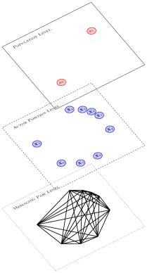
Population density process level
The message-generating actors are assumed to be members of a community, which we call the population. The aspect of the population that we model in this paper is its members’ distribution over a latent space in which the proximity between a pair of actors determines the likelihood of the pair exchanging messages. The population distribution is to be time-varying and a mixture of component distributions.
The latent space is assumed to be for some , and the population distribution at time is assumed to have a continuous density . To be more precise, we assume that the (sample) path is such that for each ,
where
-
•
is a smooth sample path of a stationary (potentially degenerate) diffusion process taking values in ,
-
•
is a probability density function on with convex support with its mean vector being the zero vector and its covariance matrix being a positive definite (symmetric) matrix,
-
•
is a smooth sample path of an -valued (potentially non-stationary or degenerate) diffusion process,
-
•
is a smooth sample path of a stationary (potentially degenerate) diffusion process taking values in .
Note that it is implicitly assumed that , and additionally, we also assume that for each and , the -th moment of the -th coordinate of is finite, i.e., .
In this paper, we take and as exogenous modeling elements. However, for an example of a model with yet further hierarchical structure, one could take a cue from a continuous time version of the classic “co-integration” theory, e.g., see Comte (1999). The idea is that the location of the -th center is non-stationary, but the inter-point distance between a combination of the centers is stationary. More specifically, one could further assume that there exist matrix , matrix and matrix such that
-
•
is the dimensional zero matrix,
-
•
is a dimensional Brownian motion,
-
•
is a stationary diffusion process.
Thus, the position of centers are unpredictable, but the relative distance between each pair of centers are as predictable as that of a stationary process.
Actor position process level
Figure 2 sketches the connection between actors and populations. We first define a process for a single actor. To begin, for each , given and , we write
where
The formulation here for the and is based on a quadratic Taylor-series approximation of a so-called “bounded confidence” model studied in Gomez-Serrano et al. (2012). Here, the value of represents the confidence level of actor on its current position and represents the visibility of other actors’ position by actor . Roughly speaking, an actor with a small value of and a large value of will be influenced greatly by actors that are positioned both near and far in the latent space whereas an actor with a large value of and a small value of will be influenced only a small amount by actors that are nearby in the latent space. For further discussion on our motivation for the form of , see Appendix A.
For each actor , the deterministic path is assumed to be continuous, taking values in a compact subset of . It is assumed that given , each actor’s latent position process is a diffusion process whose generator is , and moreover we assume that are mutually independent. For each , let
where each is assumed to be a column vector, i.e., a matrix. In other words, the -th row of is the transpose of .
Messaging process level
Denote by the number of messages sent from actor to actor . Also, denote by the number of messages exchanged between actor and actor . Note that . For each actor , we assume that the path is deterministic, continuous and takes values in . For each , we assume that
For our algorithm development and Experiment in Section 6, we take
| (1) |
but for Experiment in Section 6, we take . Next, by way of assumption, for each pair, say, actor and actor , we eliminate the possibility that both actor and actor send messages concurrently to each other. More specifically, we assume that
| (2) | |||
| (3) |
For future reference, we let
| (4) | |||
| (5) |
5 Algorithm for computing posterior processes
We denote by the conditional distribution of given , i.e., for each ,
| (6) |
For the rest of this paper, we shall assume that the (random) measure is absolutely continuous with respect to Lebesgue measure with its density denoted by . That is, for . Denote by the -th marginal posterior distribution of , i.e., for each , , and let denote its density.
5.1 Theoretical background
In Theorem 1, the exact formula for updating the posterior is presented, and in Theorem 2, our working formula used in our numerical experiments is given. We develop our theory for the case where and are the same for all actors for simplicity, as generalization to the case of each actor having different values for and is straightforward but requires some additional notational complexity.
Theorem 1.
For each and ,
where is an matrix such that for each , and for each , , and is an matrix such that for each pair , and for each pair , .
Hereafter, for developing algorithms further for efficient computations, we make the assumption that for each ,
| (7) |
where denotes the joint density for actors , and .
Theorem 2.
For each function , we have
Replacing with a Dirac delta generalized function, Theorem 2 states that for each ,
where denotes the formal adjoint operator of . For use only within Algorithm 4,
| (8) | |||
| (9) |
5.2 A mixture projection approach
The projection filter is an algorithm which provides an approximation to the conditional distribution of the latent process in a systematic way, the method being based on the differential geometric approach to statistics, cf. Bain and Crisan (2009). When the space on which we project is a mixture family, as in Brigo (2011), the projection filter is equivalent to an approximate filtering via the Galerkin method, cf. Gunther et al. (1997). Following this idea, starting from Theorem 2, we obtain below in Theorem 3 the basic formula for our approximate filtering algorithm.
To be more specific, consider a set of probability density functions . Then, let be the space of all probability density functions that can be written as a probability-weighted sum of . That is, if and only if for some probability vector on indices . In particular, for deriving our algorithms, we will assume that for some systematic choice of , each probability density under consideration is a member of .
Among many possible choices for in Theorem 3 are a multivariate Haar wavelet basis and a multivariate Daubechies basis. On the other hand, a Gaussian mixture model is pervasively used throughout statistical inference tasks such as clustering and classification in algorithms such as -means clustering. As such, we develop our algorithms with an eye towards use with other Gaussian mixture model-based algorithms. In Appendix B, we further develop our algorithm under the assumption that
where is the standard Gaussian density function defined on , , and the finite sequence is to be chosen judiciously prior to implementing the algorithm.
Preparing for our next result in Theorem 3, we let be the symmetric matrix such that , and for each , let be the symmetric matrix such that its -entry is . Collectively, we denote by the three-way tensor whose entry is . Let be the matrix such that its -entry is , where is the differential operator such that
| (10) |
with
| (11) | |||
| (12) |
Theorem 3.
Suppose that for each , and , . Let denote the column vector whose -th entry is . Then,
| (13) |
5.3 Algorithm for continuous embeddings
5.3.1 Classical multidimensional scaling
In our application, our final analysis is completed by clustering the posterior distributions. Instead of working directly with posteriors, an infinite-dimensional object, we propose to work with objects in an Euclidean space each of which represents a particular actor. However, given and , using their mean vectors or their KL distance for clustering can be uninformative. For example, if , then their mean vectors would be the same and their KL distance would be zero. However, if is the density of, say, a normal random vector such that its mean is zero and its covariance matrix is for a large value of , then concluding that actor and actor are similar could be misleading.
To alleviate such situations in a clustering step of our numerical experiments, we propose using a multivariate statistical technique called classical multidimensional scaling (CMDS) to obtain a lower dimensional representation of . More specifically, we achieve this by representing each actor as a point in , where the configuration is obtained by solving the optimization problem
| (14) |
where denotes a strictly decreasing function defined on taking values in . For example, one can take where is chosen so that for all possible values of . Another possibility among many others is to choose if is chosen so that for all possible values of .
We denote by the set of solutions to the optimization problem (14). Given a vector of probability densities on , it can be shown that the solution set is not empty and is closed under orthogonal transformations.
In the classical embedding literature, ensuring continuous embeddings is neglected as it is not relevant to their applications. However, for our work, this is crucial as we study their evolution through time, i.e., ideally, we would like to see that a small change in time corresponds to a small change in latent location. In this section, we propose an extension to the CMDS algorithm to remedy the aforementioned non-uniqueness issue, and show that the resulting algorithm ensures continuity of embeddings.
In our numerical experiments, for each , we choose a particular element of the solution set so that depends on in a consistent manner.
5.3.2 Continuous selection
By a dissimilarity matrix, we shall mean a real symmetric non-negative matrix whose diagonal entries are all zeros. First, fix such that . Then, for each dissimilarity matrix , define
where . The elements of are known as classical multidimensional scalings, and as discussed in Borg and Groenen (2005), it is well known that is not empty provided that the rank of is at least . Our discussion in this section concerns making a selection from so that the map is continuous over the set of dissimilarity matrices such that is of rank at least .
Let be a dissimilarity matrix such that the rank of is at least . We begin by choosing an element of , say , through classical dimensional scaling. Let be the eigenvalue decomposition of , where and is the diagonal matrix whose entries are the eigenvalues in non-increasing order. By the rank condition, we have . First, we formally write
| (15) |
where
- (i)
-
is the matrix with its entry ,
- (ii)
-
is the diagonal matrix whose -th diagonal entry is .
Dependence of on will be suppressed in our notation unless needed for clarity. Now, if the diagonals of are distinct, then is well defined. However, in general, due to potential geometric multiplicity of an eigenvalue, our definition of can be ambiguous. This is the main challenge in making a continuous selection and we resolve this issue in our following discussion.
For our remaining discussion, without loss of generality, we may assume that for each dissimilarity matrix , is well-defined by making an arbitrary choice if there is more than one CMDS solution. Note that the mapping may not be a continuous selection. We now remedy this. First, fix an matrix and let
where runs over all real orthogonal matrices. Then, define
| (16) |
Algorithm 5 yields the solution and the proof of the following theorem, Theorem 4, can be found in Appendix E.
Theorem 4.
Suppose that the matrix is of full column rank. Then, the mapping yields a well-defined continuous function on the space of dissimilarity matrices such that is of rank at least .

5.4 Technical observations
Here we discuss some insightful facts related to our model given the assumption stated in the last section. First, we have the following:
Theorem 5.
Fix and suppose that for a.e. . The operator is elliptic, i.e., for each , the matrix is positive definite.
Proof.
Note that for each ,
Note that and for each , and that away from a subspace of whose Lebesgue measure is zero. It follows that for each , whence is positive definite. ∎
Now, we further examine Algorithm 1, Algorithm 2, Algorithm 3, Algorithm 4, Algorithm 5, and discuss some technical points behinds these algorithms.
In Algorithm 2, existence and uniqueness of follows from Theorem 5. The continuity of follows from Theorem 5 and Strook (2008). In Algorithm 3, for simulating a sample path of , we use the so-called time-change property; that is, we use the fact that the process given by is a unit-rate simple Poisson process, where and and . For simulation, we use its dual result, i.e., is a point process whose intensity process is , where is a path of a unit-rate simple Poisson process. Also, we note that for computation of , online inference is a necessary part of our simulation in Algorithm 3; that is, we need to compute In Algorithm 3 and Algorithm 4, near-infinitesimally-small means so small that the likelihood of having more than one event during a time interval of length is practically negligible. Also, by StandardNormalVector in Algorithm 2 and UnitExponentialVariable in Algorithm 3, we mean generating, respectively, a single normal random vector with its mean vector being zero and its covariance matrix being the identity matrix, and a single exponential random variable whose mean is one.
6 Simulation experiments
In our experiments, we hope to detect clusters with accuracy and speed similar to that possible if the latent positions were actually observed even though we use only information in estimated from information contained in . We denote the end-time for our simulation as . There are two simulation experiments presented in this section, and the computing environment used in each experiment is reported at the end of this section.
Experiment 1
We take and we assume that for each and actor , and . For the population process we take for each
where
Then, we also consider , where
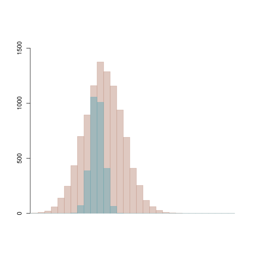
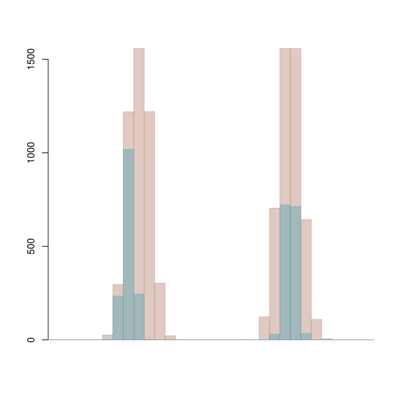
There is only one population density; in other words, . Note that even with one population center, we can have more than one empirical mode for the subpopulation. One of these modes is near zero, and another mode is near one. The reason for this is that because of the value of and , when an actor is too far away from the mode of the population process, the population process affects the actors on its tail only by negligibly small amount. In Figure 8 and Figure 7, a sample path of the true latent position of each of eight actors is illustrated in black lines. It is apparent that in the , all eight actors are equally informed of the population mode shift, but in the case, only the last three were able to adapt to the change, and the first five actors are surprised by the abrupt change at time .
Our simulation is discretized. Our unit time is , and in Figure 8, each tick in the horizontal axis corresponds to an integral multiple of . The jump term in our update formula is quite sensitive to the number of actors being considered. As such, for updating the jump term, we further discretized into subintervals for numerical stability of our update iterations. For , each unit interval is associated with sub-iterations, and the total number of the (main) iteration is , and we use instead of in each -th subiteration of each main iteration staring at time .
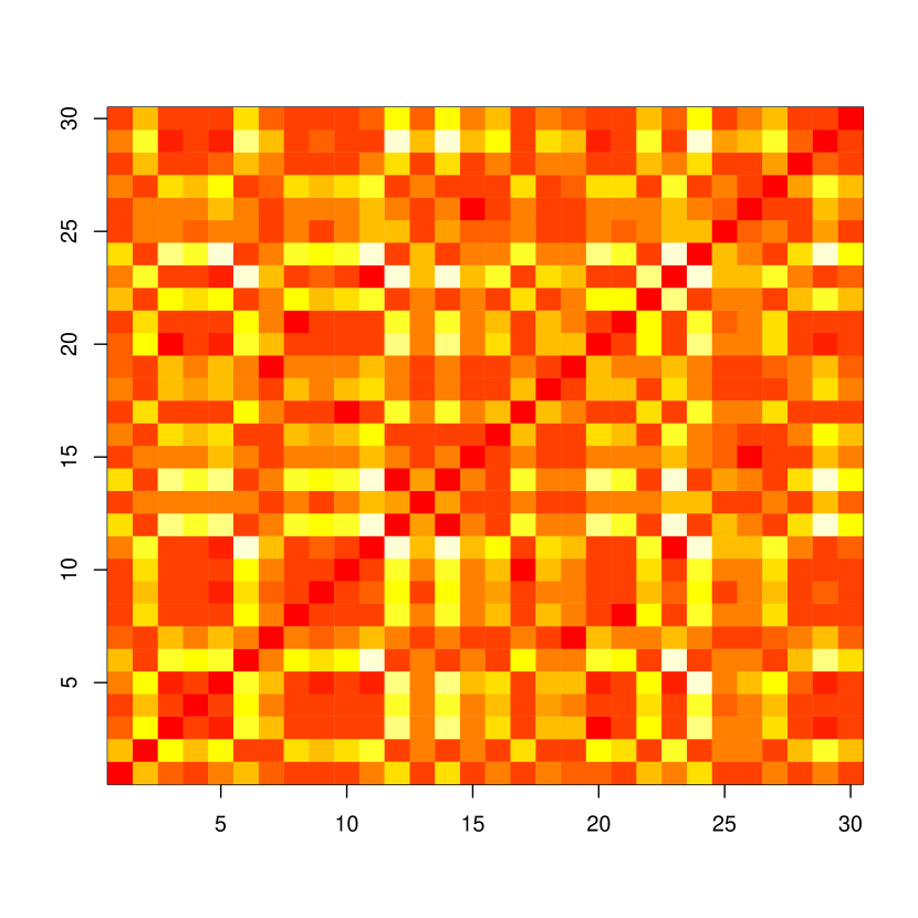
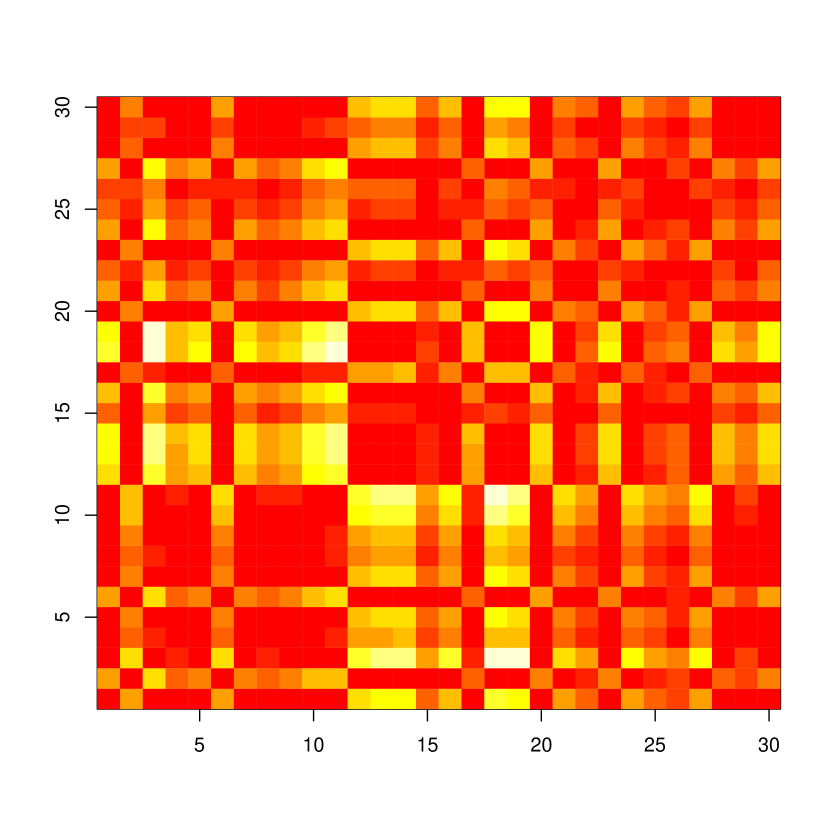
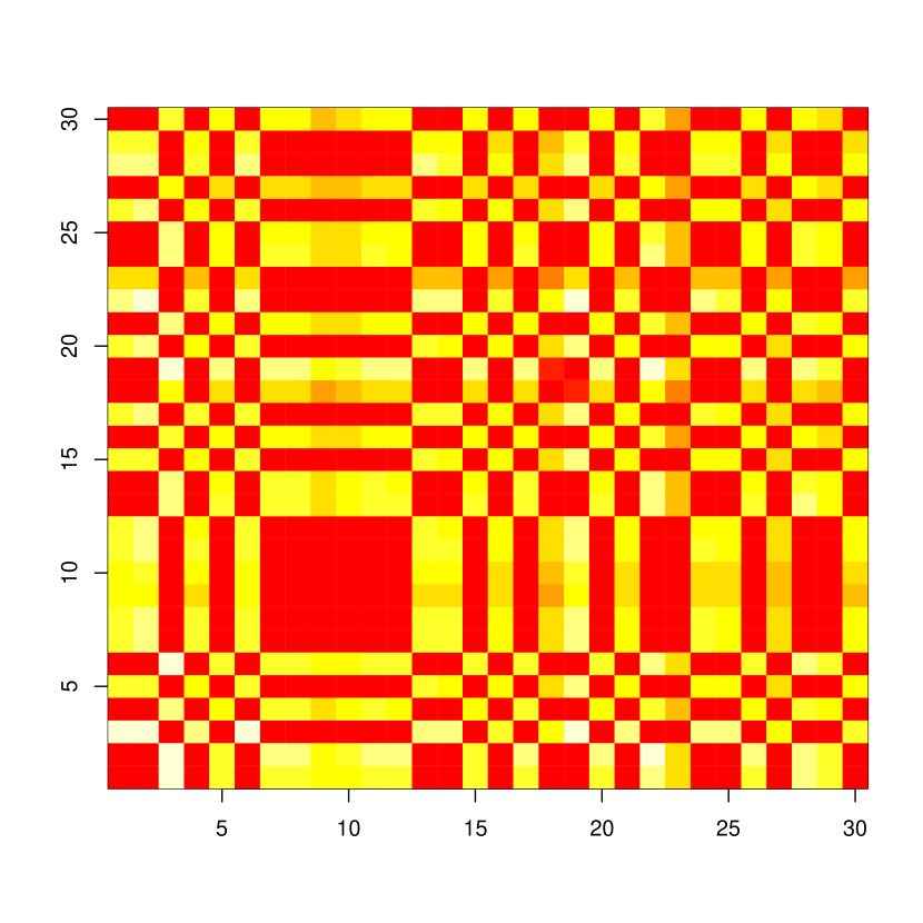
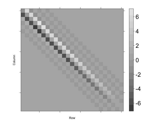
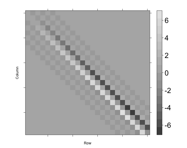
To implement our mixture projection algorithm, we take . The initial position of the actors are sampled from the initial population distribution . We take . The discretized version of is illustrated in Figure 5. For inference during our experiment, we have dropped the second order term and used only the first order term to keep the cost of running our experiment low. On the other hand, for simulating the actors’ latent positions, we have used both the first and second order term of . The value of gives the first part of the change in . Note that in both Figure 5(a) and Figure 5(b), the entries that are sufficiently far off from the diagonals are near zero.
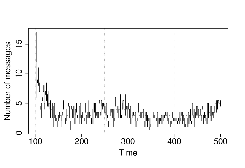
For , the time plot of the number of messages produced during interval is given in Figure 6, and shows transient behaviors of varying degrees of messaging intensity over the interval. Our set up for produced a simulation sample output of observing messages amongst the actors in unit time once the population center changed abruptly from to at the start of the -th unit time interval, i.e., . In other words, after , a single unit time is roughly associated with the amount of time during which the whole subpopulation of eight actors exchanges around messages, or equivalently, during which each pair of actors exchange around messages. On the other hand, in both and for the interval , the subpopulation messaging rate is relatively constant at the rate of messages over each unit interval, and this is expected as all eight actors are tightly situated around .
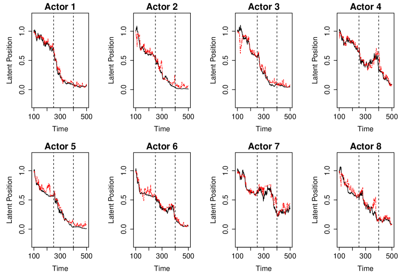
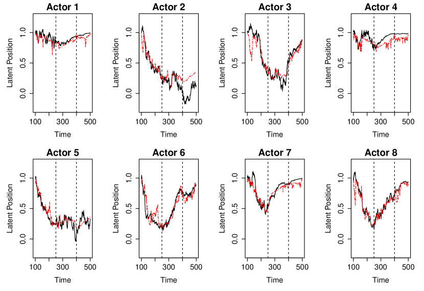
Our experiments for and
both show that the filtered positions for
all eight actors are close to the exact positions.
Experiment 2
In this experiment, for each , we have used the empirical distribution of
to obtain an estimate of by partitioning the latent space into sufficiently small intervals, where we place a uniform kernel of height equal to the proportion of that lies in that interval. Our inference is on . Recall that denotes the size of the subpopulation. The number is the size of the full population. This set-up is closer to the motivation for our work, the bounded confidence model, Gomez-Serrano et al. (2012), and the connection with our model in this paper is made in Appendix A. In theory, the general setup in Experiment 1 is comparable to the setup in Experiment 2 when in Experiment 2 is taken to be .
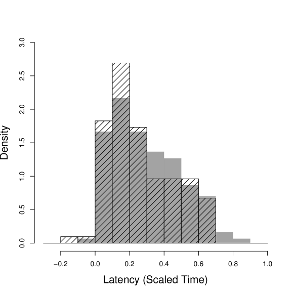
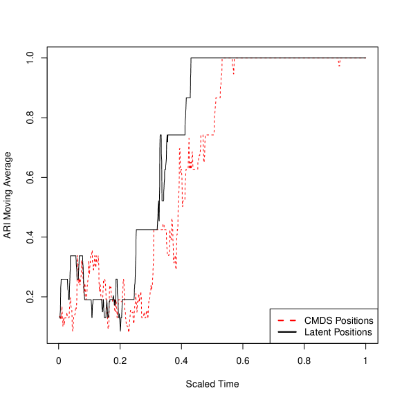
We set , , , and . We take the clustering based on as the ground truth. Note that here is comparable to in Experiment 1, or more generally, in our model. We set up the simulation to observe roughly 3000 messages amongst the actors in unit time. This translates to per actor per unit time. Note that this is a rough estimate as the messaging intensity is time-dependent and stochastic. In Figure 11, we have snapshots of and those of for a single simulation run. Denote as the latency
where the dependency on our choice for a clustering algorithm is suppressed in our notation and for some ,
where denotes a moving average of the Adjusted Rand Index (c.f. Rand (1971) and Hubert and Arabie (1985)) and we fix to be a -means clustering algorithm for concreteness. We use the latency as a performance measure for a clustering algorithm under our framework. For our projection, we use a Haar basis, i.e., a set of simple step functions, where the width of the intervals used in the experiment is . Also, unlike in Experiment 1, we take
These changes require us to modify our algorithm slightly. However, the necessary modifications are straightforward, and we leave the details to the reader.
It is important to note that we do not assume knowledge of the latent position of any individual, ; instead, we use only our knowledge of the overall population. As the number gets larger, as shown in Gomez-Serrano et al. (2012), the dependence among
diminishes, agreeing more closely with the model we specified in our framework. We investigate the behavior of our algorithm for small, medium and large values of , showing robustness of our framework in the face of limited information. Recall that Figure 11 shows results for . Figure 9 compares the latency for and . The clarity and accuracy of the clustering suffers with significant reductions in information used to estimate the priors .
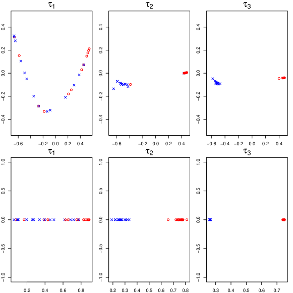
In Figure 11, we present snapshots of and for a single simulation run.
Note that is a CMDS embedding of a dissimilarity matrix
based on the posteriors . The colors denote the final cluster
membership as determined from -means clustering with . It is
clear that the emerging cluster structure of the lags
slightly behind that of in both accuracy and clarity; comparing the
middle two figures, we can see that there are a few data points misclassified
at time . Indeed, Figure 10 shows that the clustering
based on the embedded positions mirrors that possible with the true but
unobserved latent positions with a small latency.
Computing Environment
For Experiment 1, we used R 2.14.1 (64 bit) under Ubuntu 12.0.4 on an Intel Core i7 CPU 870 @ 2.93 GHz 8 machine with 16 GB RAM. For a single run for , and actors, our experiment took , and seconds respectively. For Experiment 2, we used a Red Hat Linux cluster with 24 nodes with 24 2.5 MHz CPUs and 132 GB memory each. Each Monte Carlo replicate took a single slot. A single replicate took approximately 3000 seconds.
7 Conclusion and Future Work
We have described a strategy for clustering actors based on messaging activities. Our analysis is completed by clustering a CMDS embedding of posteriors. We have presented ways to simplify posterior analysis on two levels. The first level allows us to obtain an estimate of the posteriors in an online manner. The second level allows us to reduce our analysis to studying diffusion processes, which is often a starting point for addressing the optimal stopping problem.
We have illustrated in our numerical experiments that the assumptions used to derive our two simplified approaches are mild enough to be useful for our inference task at hand, i.e., clustering.
We believe that our framework has potential for tackling the problems faced by the social network practitioner regarding emergence of structure. We intend to develop a measure of confidence for our inferred latent positions. This will be crucial to many applications, as it will provide the decision-maker with information about whether to act or to wait for more data to increase the confidence in the inferred positions. A measure of confidence would therefore be a way to establish a stopping rule. Noting that we took the parameters of our model to be exogenous, we will need to explore robustness of our inference to incorrect parameter choices and then make explicit an algorithm for parameter estimation. Making our algorithm more scalable is also an area of our interest. These areas of future work will be key to applying our framework on substantial problems.
Acknowledgements
This work is partially supported by a National Security Science and Engineering Faculty Fellowship (NSSEFF), by the Acheson J. Duncan Fund for the Advancement of Research in Statistics, and by the Johns Hopkins University Human Language Technology Center of Excellence (JHU HLT COE). We also thank Dr. Youngser Park for his technical assistance.
Appendix A Motivation for the form of the differential operator
A.1 Bounded confidence model: an adaptation
Our work in this paper is in part influenced by a so-called bounded confidence model in Gomez-Serrano et al. (2012) which focuses on establishing a propagation of chaos property of the interacting particles model studied there. When denoting the actors’ latent positions , in the bounded confidence model, the opportunities for (latent) position changes that each actor experiences is modeled as a simple Poisson process. When there is a change at time , the change is assumed to involve precisely two actors, say, actor and actor , such that their position and differs by at most . This yields an inhomogeneity in the rate at which actors change their locations. Then, the exact amount of change is specified by the following formula:
where is a fixed constant. Roughly speaking, upon interaction, actor keeps percent of its original position, and is allowed to be influenced by percent of the original position of actor , and vice versa.
Fix constants and . Then, define by letting for each and ,
Studied in Gomez-Serrano et al. (2012) particularly is the interaction between and where is the empirical distribution of . As shown in Gomez-Serrano et al. (2012), the bounded confidence model has an appealing feature that the parameter space for the underlying parameters and can be partitioned according to the type of consensus that the population eventually reaches, namely, a total consensus and a partial consensus. In a total consensus regime, for sufficiently large , everyone is expected to gather tightly around some fixed common point . On the other hand, in a partial consensus regime, (depending on and ), there is a finite collection of distinct values in separated by at least , to exactly one of which each actor’s position is attracted. In particular, the (asymptotic) position of actors yields a partition of the actor set when the exact locations of are known. Generally, is contracting toward for some closed convex non-empty disjoint subsets and of in the sense that for some , for each and .
In our adaptation, for analytic tractability, we replace the indicator function with , take to be an exogenous modeling element, and take to be potentially time dependent, yielding the operator
| (17) |
The second numerical experiment in Section 6 focuses on the case where the community starts with no apparent clustering but as time passes, each actor becomes a member of exactly one of clusters, where each cluster is uniquely identified by a closed convex subset of the latent space .
A.2 A quadratic Taylor series approximation
In this work, we use a model that that captures the action in (17) up to the second order. To begin, note that
where and denote respectively the gradient and the Hessian of at , and H.O.T. denotes the higher order terms. Suppose that is given. Now, we have
where and are given by the following:
Dropping the term associated with H.O.T., we obtain the following:
Appendix B The mixture projection filter formula
B.1 Proof of Theorem 3
For each , we see that
We first consider the second term of the right side of (13).
Now, we have that
and that
Hence,
Next, for the first term of the right side of (13), we have
In summary, for each , we have
and our claim follows from this.
B.2 Preliminary lemmas
This section contains two formulas to be used in the next section. Our result and proof in Lemma 7 is stated in the same notation as in Lemma 6. Recall that .
Lemma 6.
Let and . Then,
where is the Gram matrix for and is the matrix whose -entry is .
Proof.
Let and for each , let . First, note that
Now,
Our claim follows from this. ∎
Lemma 7.
Let be the standard multivariate normal density defined on . Also, fix a sequence , and a sequence .
Proof.
B.3 Formula for in a multivariate normal density case
Here, we assume, as done in Theorem 3, that and , where for simplicity, we have written . In this section, we fix to be the standard multivariate normal density defined on and recall that . Also, we fix , and a sequence .
Lemma 8.
Fix , and . For each ,
| (18) | |||
| (19) |
Proof.
Let
where to simplify the expression of , we have used the fact that
Also, note that
Using Lemma 7 with , and , we see that
Then, for our claim in (18), it is enough to see that
Next, we show our claim in (19). Hereafter, to ease our notation, we write for . First, for , we have
and hence,
On the other hand, for , we have
and so, we have
Our claim in (19) follows. ∎
For Lemma 9 and Lemma 10, by , we denote the Gram matrix for , and define to be as in Lemma 6 for , , . Let
To simplify our notation, we let
Define and note
Also, denote by the multivariate normal density defined on such that its mean vector is and its covariance matrix is . For and , we write
and note that in particular,
Lemma 9 and Lemma 10 are associated, respectively, with the first and the second terms appearing in the right side of (20).
Lemma 9.
For each and , we have
Proof.
To ease our notation, we first let
It follows that
| (21) | |||
| (22) |
We compute instead of directly working with (11). First, we observe that
and that
Using Lemma 6 on the third equality, we see that
Continuing with the calculation,
| (23) | |||
| (24) | |||
| (25) |
Putting together (23), (24), (25) and (22), and plugging in the full expression for , we see that
Our claim follows after summing over and replacing with its full expression. ∎
Lemma 10.
For each , and ,
Proof.
Note that
where
We first compute the diagonal terms, i.e., the cases. Note that
and also that
Next, we compute the off-diagonal terms, i.e., the cases. First, using our calculation just above, we see that we note that
Our claim follows from this after combining them together, and simplifying the combined term into a matrix notation. ∎
Appendix C Proof for Theorem 1
Here, we will take the convention that is organized as a matrix. By the -th row of , we mean . Let
where for each and ,
In other words, is the (random) conditional characteristic function of . Note
Also, let, for each and ,
| (26) |
For each , denotes the function obtained by fixing all other indices different from the -th actor indices but letting the -th actor indices to be free, and if is in the domain of the operator , with some abuse of notation, we write:
Similarly, for each , let
In other words, denotes the conditional characteristic function of the -th row of , and also, let, for , and ,
| (27) |
Note that the definition of is actually independent of a particular choice of vertex as they are all identically distributed.
One can prove the next result by directly following Snyder (1975), but one needs to adapt to the fact that the underlying process can now be a time-inhomogeneous non-linear Markov process. The proof details are left to the reader. For a survey of similar techniques, see also Kunita (1997) and Bain and Crisan (2009).
Proposition 11.
For each and ,
Our proof of Theorem 1 is by brute force calculation, starting from Proposition 11. In particular, our claim in Theorem 1 follows from Proposition 11 by directly applying Lemma 12, Lemma 13 and Lemma 14 which we list and prove now.
Lemma 12.
For each ,
Proof.
Fix , , and . Then, for each , we have:
We have
and hence,
It follows that
∎
Lemma 13.
For each , we have:
Proof.
Fix and note:
and that
Treating as a generalized function (i.e. a tempered distribution), we have:
∎
Lemma 14.
For each , we have:
Proof.
Note
∎
Appendix D Proof of Theorem 2
Recall that for each , denotes the function obtained by fixing all other indices different from the -th actor indices but letting the -th actor indices to be free. Fix . Let be such that for all . For each ,
Then, the claimed formula follows from our assumption in (7).
Appendix E Proof of Theorem 4
Suppose that as and that for each , satisfies the rank condition, i.e., is of rank at least . Note that each is a non-empty compact subset of since for any real orthogonal matrix . In particular, for sufficiently small , we may assume that . It is enough to show that for each arbitrary convergent subsequence of ,
| (28) |
Consider an arbitrary convergent subsequence of . We begin by observing some linear algebraic facts. First, any sequence of real orthogonal matrices has a convergent subsequence whose limit is also real orthogonal. Next, since both and are of rank , there exists a unique real orthogonal matrix such that
and in fact, where is a singular value decomposition of , and is the corresponding unique right factor in the polar decomposition of . Note that this implies the well-definition part of our claim on . Also, since , we have that
For relevant linear algebra computation details for these facts, see Horn and Johnson (1985, pg. 69, pg. 370, pg. 412, and pg. 431).
Now, by taking a subsequence if necessary, we also have that for some matrix such that , . Then,
Next, note that if has distinct diagonal elements, then we also have so that . On the other hand, more generally, i.e., even when there are some repeated diagonal elements, we can find a matrix such that . To see this, note that the -th column of is also an eigenvector of for the eigenvalue , and , and hence it follows that for some real orthogonal matrix , we have . Moreover, exploiting the block structure of owing to algebraic multiplicity of eigenvalues, we can in fact choose so that . Then,
Now, we have
where is a real orthogonal matrix and and implicitly the limit was taken along a further subsequence when necessary. Moreover,
In summary, we have:
By definition of , along with the facts that (i) all of the convergent subsequences share the common limit, (ii) each subsequence has a convergent subsequence, and (iii) and have of full column rank , we have (28).
References
- Adamic and Adar [2005] L. Adamic and E. Adar. How to search a social network. Social Networks, 27:187–2003, 2005.
- Andersen et al. [1995] P. K. Andersen, O. Borgan, R. Gill, and N. Keiding. Statistical Models Based on Counting Processes. Springer, 1995.
- Bain and Crisan [2009] A. Bain and D. Crisan. Fundamentals of Stochastic Filtering. Springer, 2009.
- Borg and Groenen [2005] I. Borg and P. J. F. Groenen. Modern Multidimensional Scaling: Theory and Applications. Springer, 2005.
- Bremaud [1981] P. Bremaud. Point processes and queues. Springer-Verlag, 1981.
- Brigo [2011] D. Brigo. The direct geometric structure on a manifold of probability densities with applications to filtering. 2011. URL http://arxiv.org/abs/1111.6801.
- Chi and Kolda [2012] E. Chi and T. Kolda. On Tensors, Sparsity, and Non-negative Factorizations. SIAM Journal on Matrix Analysis and Application, 33(4), 2012.
- Choudhury et al. [2010] M. De Choudhury, W. Mason, J. Hofman, and D. Watts. Inferring relevant social networks from interpersonal communication. In In Proc. 19th Intl Conf. World Wide Web, New York, pages 301—310. Association for Computing Machinery, 2010.
- Comte [1999] F. Comte. Discrete and continuous time cointegration. Journal of Econometrics, (88):207–226, 1999.
- Cortes et al. [2003] C. Cortes, D. Pregibon, and C. Volinsky. Computational methods for dynamic graphs. Journal of Computational and Graphical Statistics, 12:950–970, 2003.
- Eckmann et al. [2004] J.-P. Eckmann, E. Moses, and D. Sergi. Entropy of dialogues creates coherent structure in e-mail traffic. Proceedings of the National Academy of Sciences of the United States of America, 101:14333–14337, 2004.
- Gomez-Serrano et al. [2012] J. Gomez-Serrano, C. Graham, and J.-Y. Le Beudec. The Bounded Confidence Model of Opinion Dynamics. Mathematical Models and Methods in Applied Sciences, 22, 2012.
- Gunther et al. [1997] J. Gunther, R. Beard, J. Wilson, T. Oliphant, and W. Stirling. Fast Nonlinear Filtering via Galerkin’s Method. In Proceedings of the American Control Conference, 1997.
- Heard et al. [2010] N. Heard, D. Weston, K. Platanioti, and D. Hand. Bayesian anomaly detection methods for social networks. Ann. Appl. Statist., 4:645–662, 2010.
- Horn and Johnson [1985] R. Horn and C. Johnson. Matrix analysis. Cambridge, 1985.
- Hubert and Arabie [1985] L. Hubert and P. Arabie. Comparing partitions. Journal of the Classification, 1985.
- Kunita [1997] H. Kunita. Stochastic flows and stochastic differential equations. Cambridge University Press, 1997.
- Lee and Maggioni [2011] J. D. Lee and M. Maggioni. Multiscale Analysis of Time Series of Graphs. In Proc. SampTA, 2011.
- Lee and Priebe [2011] N. H. Lee and C. E. Priebe. A Latent Process Model for Time Series of Attributed Random Graphs. Statistical Inference for Stochastic Processes, 14(3):231–253, October 2011.
- Perry and Wolfe [2013] P. Perry and P. Wolfe. Point process modelling for directed interaction networks. Journal of the Royal Statistical Society, Series B, 2013. URL http://arxiv.org/abs/1011.1703.
- Rand [1971] W. Rand. Objective Criteria for the Evaluation of Clustering Methods. Journal of the American Statistical Association, 1971.
- Ranola et al. [2010] J. Ranola, S. Ahn, M. Sehl, D. Smith, and K. Lange. A Poisson model for random multigraphs. Bioinformatics, 26, 2010.
- Snyder [1975] D. Snyder. Random point processes. John Wiley & Sons Inc, 1975.
- Stomakhin et al. [2011] A. Stomakhin, M. Short, and A. Bertozzi. Reconstruction of missing data in social networks based on temporal patterns of interactions. Inverse Problems, 2011.
- Strook [2008] D. W. Strook. Partial Differential Equations for Probablist. Cambridge University Press, 2008.
- Tang et al. [2013] M. Tang, Y. Park, N. H. Lee, and C. E. Priebe. Attribute Fusion in a Latent Process Model for Time Series of Graphs. IEEE Transactions on Signal Processing, 61(7):1721–1732, 2013.