A Hough Transform Approach to Solving Linear Min-Max Problems

Several ways to accelerate the solution of 2D/3D linear min-max problems in $n$ constraints are discussed. We also present an algorithm for solving such problems in the 2D case, which is superior to Cgal’s linear programming solver, both in performance and in stability.

1 Purpose

This work is focused on several ways to accelerate the solution of 2D/3D linear min-max problems in $n$ constraints. We also present an algorithm for solving such problems in the 2D case, which is superior to Cgal’s linear programming solver, both in performance and in stability.

Problem 1.

Linear Min-Max problem, also known as $L_{\infty}$ linear optimization

$$\arg\min_{x,y\in\mathbb{R}}\left(\max_{i\in\left[n\right]}\left|a_{i}x+b_{i}y+c_{i}\right|\right)=\arg\min_{x,y}\left(\left\|M\cdot\left(x,y,1\right)^{T}\right\|_{\infty}\right),$$

where $M=\left[a|b|c\right]$.

This problem can be re-written as a Linear Programming of the following form.

Problem 2.

$$\mbox{minimize}_{x,y,t} t$$

s.t $$a_{1}x+b_{1}y+c_{1}\leq t$$

$$\,\,\,\,\,\,\,\,\,\,\,\,\,\,\vdots$$

$$a_{n}x+b_{n}y+c_{n}\leq t.$$

It is known for several decades (Megiddo (1984)) that general Linear Programming problems (and thus, also linear min-max problems) can be solved in $\mathcal{O}\left(n\right)$ time when the dimension is constant. Therefore, there is only hope to demonstrate a constant factor acceleration; however, in real applications, this can be valuable.

2 The Hough Transform

We begin with a quick overview of a natural extension to the Hough Transform Hough (1962) to 3D. We note that the following theorems, although proved for 3D, hold equally well in 2D; the proofs are identical if we rename the $z$ coordinate into $y$.

Given a point $p=\left(a,b,c\right)$ in $\mathbb{R}^{3}$, we define its dual plane as $\mathcal{H}\left(p\right)=\ell\left(x,y\right)=ax+by-c$, and given a plane $\pi\left(x,y\right)=ax+by+c$, we define its dual point as $\mathcal{H}\left(\pi\right)=\left(a,b,-c\right)$. The usefulness of these definitions is highlighted in the following lemmas.

Lemma 3.

A point $p=\left(x_{0},y_{0},z_{0}\right)$ is above a plane $\pi\left(x,y\right)=ax+by+c$ iff the plane $\mathcal{H}\left(p\right)$ is below the point $\mathcal{H}\left(\pi\right)$. Moreover, $p$ is on $\pi$ iff $\mathcal{H}$$\left(\pi\right)$ is on $\mathcal{H}\left(p\right)$.

Proof.

We know that $\pi\left(x_{0},y_{0}\right)=x_{0}a+y_{0}b+c<z_{0}$; by definition of the Hough transform, $\left[\mathcal{H}\left(p\right)\right]\left(\mathcal{H}\left(\pi\right)_{x},\mathcal{H}\left(\pi\right)_{y}\right)=x_{0}\mathcal{H}\left(\pi\right)_{x}+y_{0}\mathcal{H}\left(\pi\right)_{y}-z_{0}$ which equals $x_{0}a+y_{0}b-z_{0}$. Because $x_{0}a+y_{0}b+c<z_{0}$, we must have $x_{0}a+y_{0}b-z_{0}<-c$, concluding that $\left[\mathcal{H}\left(p\right)\right]\left(\mathcal{H}\left(\pi\right)_{x},\mathcal{H}\left(\pi\right)_{y}\right)<\mathcal{H}\left(\pi\right)_{z}$. A very similar argument can be used to show that a point is on a plane iff its dual is on its dual. ∎

Lemma 4.

The upper envelope of a set of planes corresponds to the lower convex hull of the planes’ dual points.

Proof.

By definition, a point $p$ on the upper envelope of a set of planes $\left\{\pi_{i}\right\}$ is above all of them (except several on which it lies), and by Lemma 3 we have that the plane $\mathcal{H}\left(p\right)$ is below all the points $\mathcal{H}\left(\pi_{i}\right)$ (except several which it touches). The converse is also true - every plane $\pi$ that is part of the lower convex hull is lower than all points $p_{i}$ (except several which it touches), therefore $\mathcal{H}\left(\pi\right)$ must be above all the planes $\mathcal{H}\left(p_{i}\right)$. ∎

We will henceforth denote the convex hull of a set of points $P$ by $\mathcal{CH}\left(P\right)$, and its lower convex hull by $\mathcal{LH}\left(P\right)$. Figure 1 demonstrates the above lemmas in the 2D case.

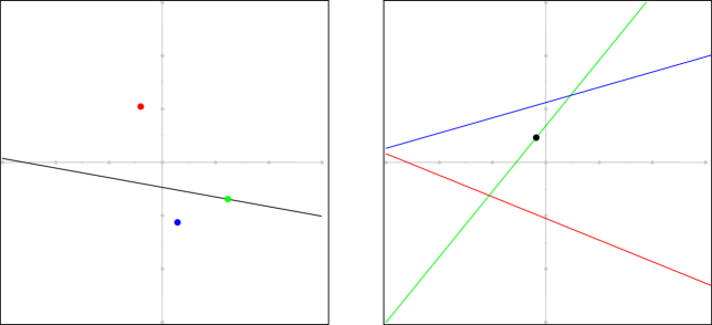
Figure 1: Hough Transform of three points and a line (plane in 3D). Lines and points, and their duals, are related by their color.

3 A Linear Min-Max Problem in the Hough space

Solving the linear program is equivalent to finding the lowest point of the upper envelope of the set of planes defined by

$$z_{k}\left(x,y\right)=a_{k}x+b_{k}y+c\,\,\,\,k=1,2,\dots,n.$$

We saw that the upper envelope corresponds to the lower convex hull of the set of points $DP=\left\{\left(a_{k},b_{k},-c_{k}\right)\right\}_{k=1}^{n}$. It is now obvious that a solution to Problem 2, which is a point $\left(x,y,t\right)$ on the upper envelope, corresponds to a plane in the dual space, which is defined by a face of $\mathcal{LH}\left(DP\right)$.

Consider an optimum for the target function of the linear problem, namely $t_{opt}$, and define the following plane which is parallel to the $x-y$ plane: $\pi\left(x,y\right)=0\cdot x+0\cdot y+1\cdot t_{opt}$. The dual to this plane, $\mathcal{H}\left(\pi\right)$, is a point on the $z$ axis. Because the optimal solution $p$ to Problem 2 is a point that is on $\pi$, its dual $\mathcal{H}\left(p\right)$ is a plane on which the point $\mathcal{H}\left(\pi\right)$ must be. This means that the dual to the plane that has the highest intersection with the $z=0$ axis (and is part of $\mathcal{LH}\left(DP\right)$) is the solution to the linear program. Moreover, it is obvious that if there is a face of the lower convex hull that intersects the $z$ axis, it has the highest intersecting plane. If there is no such face, either all of the points have a positive $a_{k}$, or all have a negative $a_{k}$, which means the problem is unbounded.

The last two statements suggest that solving our linear program is equivalent to finding the face of the lower convex hull that intersects the $z$ axis. Unfortunately, we are unaware of an $\mathcal{O}\left(n\right)$ method to do so.

Figure 2 demonstrates the above lemmas in the 2D case.

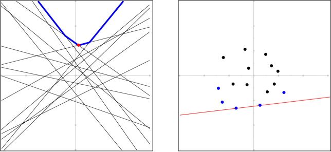
Figure 2: Left: a linear min-max problem, and its solution (red point). Right: duals of planes defining the problem, and the dual to the solution (red line).

4 The 2D Case: Solving Problem 2 in the Hough plane

Although the last section ends in a pessimistic note, this section provides an algorithm which in practice, solves 2D linear min-max problems much faster than Cgal’s solve_linear_program Fischer et al. (2011). We were unable, at the time of writing this work, to provide a complexity proof; however, experiments support the conjecture it is linear in the number of constraints. See Figure 3

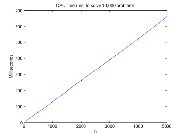
Figure 3: CPU time in milliseconds to solve 10,000 random problems with $n$ constraints (our algorithm)

To clarify: we remove the $y-$coordinate from our problem formulation and rename $z$ into $y$, to obtain the following class of problems:

$$\mbox{minimize}_{x,t} t$$

s.t $$a_{1}x+b_{1}\leq t$$

$$\,\,\,\,\,\,\,\,\,\,\,\,\,\,\vdots$$

$$a_{n}x+b_{n}\leq t.$$

The algorithm is as follows.

Input: A set of $n$ constraints: $a_{i}x+b_{i}\leq t,\,\,\,\,i\in\left[n\right]$

Output: Optimal primal point $\left(x,t\right)$

1. Transform constraints into a set of points $DP$

2. Partition $DP$ into $L$ (points with negative $x-$coordinate) and $R$ (positive)

3. Pick some point $p_{0}\in L$

4. Repeat until no change:

   1. Given $p_{i}$ in $L$ ($R$), find a point $p_{i+1}$ in $R$ ($L$) with the largest clockwise (counter-clockwise) turn from $p_{i}$.

5. Compute the line that intersects the last two points $p_{k}$ and $p_{k+1}$: $\ell\left(x\right)=mx-mp_{k}^{\left(x\right)}+p_{k}^{\left(y\right)}$ where $m=\left(p_{k+1}^{\left(y\right)}-p_{k}^{\left(y\right)}\right)/\left(p_{k+1}^{\left(x\right)}-p_{k}^{\left(x\right)}\right)$

6. Compute the dual to this plane: $\left(m,mp_{k}^{\left(x\right)}-p_{k}^{\left(y\right)}\right)$

7. Return either (6) or $-\infty$.

Algorithm 1 Solving in Hough plane (2D)

First, we should prove the algorithm takes a finite number of steps.

Claim 5.

Step (4) in Algorithm 1 terminates.

Proof.

Suppose we are at step $i+1$, and the last two points are $p_{i}$ and $p_{i+1}$. Also assume without loss of generality that $p_{i}\in L$ and therefore $p_{i+1}\in R$. Next, either step (4a) terminates (we’re done) or a new point $p_{i+2}\in L$ is selected. The criterion for the selection is that $p_{i+2}$ constitutes a counter-clockwise turn from $p_{i}$, which is equivalent to to the line $\left(p_{i+2},p_{i+1}\right)$ having a larger inclination than the line $\left(p_{i},p_{i+1}\right)$. However, because both lines intersect $p_{i+1}$, and the second one has a larger inclination, its intersection with the $y$ axis is smaller than that of the first one. This means that the $y-$intersection of any $\left(p_{i},p_{i+1}\right)$ is smaller than the $y-$intersection of any line $\left(p_{j},p_{j+1}\right)$ for all $i>j$. Because the number of points is finite, the minimum of $y-$intersections of lines defined by any pair of points in $DP$ is finite, therefore step (4a) terminates. ∎

We are left with showing that when step (4a) terminates, the points $p_{k}$ and $p_{k+1}$ are indeed part of $\mathcal{LH}\left(DP\right)$; the fact that the segment $\left(p_{k},p_{k+1}\right)$ intersects the $y$ axis is obvious.

Proof.

Assume without loss of generality that $p_{k}\in L$ and therefore $p_{k+1}\in R$. By step (4a) we know that no point in $R$ has a clockwise turn from the line $\left(p_{k},p_{k+1}\right)$, or equivalently, that all the points in $R$ are above this line. Similarly, no point in $L$ is above this same line for symmetric reasons. This means this line supports $DP$ (from below), which means it must be on its lower convex hull. ∎

Figure 4 demonstrates the algorithm.

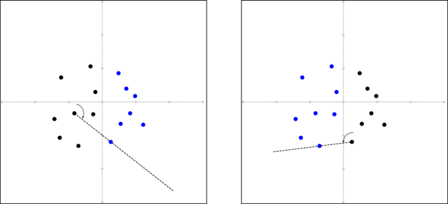
Figure 4: Two applications of step 4a

4.1 Experimental Verification

We pit our algorithm against Cgal’s linear programming solver Fischer et al. (2011). The constraints were drawn from a 2D Gaussian random variable $X\sim\left[N\left(E=0,\sigma^{2}=10\right)\right]^{2}$. As is evident in Figure 5 which depicts the ratio between running times of the two solvers, versus the number of constraints $n$, the new algorithm is about 10 times faster than Cgal’s.

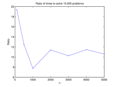
Figure 5: Ratio of time to solve 10,000 problems, vs. problem size ($n$)

4.1.1 Implementation notes

Our solver only uses addition and multiplication and is highly-parallelizable. No divisions are used, which results in a faster and more stable solver.

Cgal’s solver requires the use of so-cold exact types, such as rational numbers or arbitrary-precision floating point numbers; the use of such types is extremely slow at this time, because of the way Cgal uses them. Therefore, the solver was tricked to using simple machine double-precision floating point numbers. This resulted in numerical failure when the number of constraints $n$ was greater than $\approx 10^{5}$. Our solver, however, is working even with this number of constraints. Moreover, the only numerically sensitive step in our algorithm is in Step (4a), which involves deciding if three points define a clockwise turn. This is done by computing $\left(p_{1}-p_{0}\right)\wedge\left(p_{2}-p_{0}\right)\overset{?}{>}0$, which can be done by setting $\tilde{p}_{i}=p_{i}-p_{0}$ and then deciding if

$$\tilde{p}_{1}^{x}\cdot\tilde{p}_{2}^{y}\mbox{ is greater than }\tilde{p}_{1}^{y}\cdot\tilde{p}_{2}^{x},$$

or equivalently,

$$\frac{\tilde{p}_{1}^{x}}{\tilde{p}_{1}^{y}}\mbox{ is greater than }\frac{\tilde{p}_{2}^{x}}{\tilde{p}_{2}^{y}}.$$

This comparison can be performed in exact by converting each fraction to a continued fraction, which is still much faster than using an arbitrary-precision floating point number.

A computer using Core 2 Quad (Q9400) @ 2.66 GHz and 6GB RAM was used for the benchmarking. 10,000 random problems were solved by each of the solvers, and their results compared.

5 The 3D Case: Discarding of Constraints

To again recede to a pessimistic note, we were unable to extend the 2D algorithm into 3D. However, modifying the problem at hand allows us to quickly and safely discard of some of the constraints. The modified problem has two more constraints: the solution point $\left(x,y,t\right)$ must have its coordinates $x$ and $y$ between 0 and 1.

Problem 6.

$$\mbox{minimize}_{x,y,t} t$$

s.t $$a_{1}x+b_{1}y+c_{1}\leq t$$

$$\,\,\,\,\,\,\,\,\,\,\,\,\,\,\vdots$$

$$a_{n}x+b_{n}y+c_{n}\leq t$$

$$x\in\left[0,1\right]$$

$$y\in\left[0,1\right].$$

This problem is indeed very specific, but is in the core of the GMDS algorithm Bronstein et al. (2006) in the $L_{\infty}$ norm, where $x$ and $y$ represent barycentric coordinates inside a triangle.

To reiterate, solving Problem 6 is equivalent to finding the face of the 3D lower convex hull of the points which are dual to the planes defined by the constraints, which intersects the $z$ axis. In addition, if this (only) plane $z\left(x,y\right)=ax+by+z$ has either $a\notin\left[0,1\right]$ and/or $b\notin\left[0,1\right]$, the solution must be on the boundary of the feasible set.

In other words, it is possible to discard of all of the points in $DP$ which support planes with either $a\notin\left[0,1\right]$ and/or $b\notin\left[0,1\right]$ and not change the solution, provided that the boundaries of the feasible set are checked. We note that $a$ corresponds to the inclination in the $x$ direction, and $b$ to the inclination in the $y$ direction.

To illustrate the points which can be discarded, consider a simplification of the problem to 2D. Figure 6 shows a set of points for which we should find a line that supports the rest of the points, from below, and has the highest $y-$intersect. Surely, we can discard of the points on the left of the lowest point, because these points are either interior, or support segments of $\mathcal{LH}\left(DP\right)$ which have negative inclinations. Also, points on the right of the lowest point, which define lines with inclination greater than 1 can also be discarded.

Figure 6: Points in red only support segments which have a negative inclination. Blue ones only support segments with inclinations greater than 1.

The last two statements are true in 2D, but not necessarily in 3D - removing points changes the convex hull, and there is danger that the new convex hull will introduce bogus solutions to the problem. We will see later that this is not the case, and removing the points is indeed safe.

The main result is detailed in Theorem 12, which is based on the following propositions.

Definition 7.

A point $p=\left(p_{x},p_{y},p_{z}\right)$ is behind another point $q=\left(q_{x},q_{y},q_{z}\right)$ if $p_{x}<q_{x}$, $p_{y}<q_{y}$ and $p_{z}>q_{z}$.

Proposition 8.

Let $p^{min}\in DP$ be a point with a minimal $z-$coordinate, and let $p\in DP$ be point which is behind $p^{min}$. Then any plane defined by $n\cdot\left(q-p\right)=0$ that:

1. Goes through $p$,

2. Supports $\mathcal{CH}\left(DP\right)$, that is, for any point $q\in DP$ we have $n\cdot\left(q-p\right)\geq 0$, and;

3. Has a positive $z-$coordinate $n_{z}$

cannot be a solution to Problem 6 , because its dual point has negative $x$ and/or $y$ coordinate.

Proof.

Apply Requirement (2) to the point $q=p^{min}$, for which $q-p$ equals $\left(+\alpha,+\beta,-\gamma\right)$ for some positive $\alpha,\beta$ and $\gamma$. The result is the relation $n_{x}\alpha+n_{y}\beta>n_{z}\gamma$, which forces either of $n_{x}$ or $n_{y}$ to be positive. Now, because $\left(n_{x},n_{y},n_{z}\right)$ is a normal to a plane, the corresponding plane equation must be $n_{z}\cdot z\left(x,y\right)=\left(-n_{x}\right)x+\left(-n_{y}\right)y+c$ for some constant $c$. Because $n_{z}$ is positive by Requirement (3), either of the coefficients of the plane must be negative, which means the dual to this plane cannot be a solution to Problem 6. ∎

We can state a similar result for points which are “too steep” with respect to $p^{min}$.

Definition 9.

A point $p=\left(p_{x},p_{y},p_{z}\right)$ is too steep with respect to another point $q=\left(q_{x},q_{y},q_{z}\right)$ if $p\succ q$ (larger in all coordinates), and

$$\frac{p_{z}-q_{z}}{p_{x}-q_{x}}>1\mbox{ and }\frac{p_{z}-q_{z}}{p_{y}-q_{y}}>1.$$

Proposition 10.

Let $p^{min}\in DP$ be a point with a minimal $z-$coordinate, and let $p\in DP$ be a point which is too steep with respect to $p^{min}$. That is, with all coordinates larger than those of $p^{min}$ such that the vector $p^{min}-p=\left(-\alpha,-\beta,-\gamma\right)$, $\alpha,\beta$ and $\gamma$ positive, satisfies

$$\alpha<\gamma\mbox{ and }\beta<\gamma.$$

Then any plane defined by $n\cdot\left(q-p\right)=0$ that:

1. Goes through $p$,

2. Supports $\mathcal{CH}\left(DP\right)$, that is, for any point $q\in DP$ we have $n\cdot\left(q-p\right)\geq 0$, and;

3. Has a positive $z-$coordinate $n_{z}$

cannot be a solution to Problem 6, because its dual point has its $x$ and/or $y$ coordinate larger than 1.

Proof.

In a similar way to the proof of Proposition 8, we obtain

$$\left(n_{x},n_{y},n_{z}\right)\cdot\left(-\alpha,-\beta,-\gamma\right)=\left(-n_{x}\right)\alpha+\left(-n_{y}\right)\beta-n_{z}\gamma,$$

which implies

$$\left(-\frac{n_{x}}{n_{z}}\right)\alpha+\left(-\frac{n_{y}}{n_{z}}\right)\beta>\gamma.$$

We can normalize $n$ such that $n_{z}$ will be 1, without changing its sign, because $n_{z}$ is positive by Requirement (3):

$$\left(-n_{x}\right)\frac{\alpha}{\gamma}+\left(-n_{y}\right)\frac{\beta}{\gamma}>1.$$

Now, if both $\alpha/\gamma$ and $\beta/\gamma$ are smaller than 1, $n_{x}$ and $n_{y}$ cannot be both larger than -1. Noting that the explicit plane equation which the normal vector $n$ (with $n_{z}=1$) induces is $z\left(x,y\right)=\left(-n_{x}\right)x+\left(-n_{y}\right)y+c$ for some $c$, leads to the conclusion that at least one of the coefficients of the plane must be larger than 1, and therefore its dual point cannot be a solution to the linear program. ∎

We state a simple characterization of lower convex hulls :

Lemma 11.

Any plane $\pi$ defined by $n\cdot\left(q-p\right)=0$, which supports $\mathcal{LH}\left(DP\right)$ must have a positive $z-$coordinate of $n$ , $n_{z}$.

Proof.

Since $\pi$ is part of the lower convex hull, there must be a pair of points $q_{1}$ and $q_{2}$ such that $q_{1}$ is on $\pi$, and $q_{2}=q_{1}+\epsilon\left(0,0,1\right)$; therefore, the condition $n\cdot\left(q_{1}-q_{2}\right)>0$ forces $n_{z}>0$. ∎

We are now ready to show that we can safely discard of a class of constraints.

Theorem 12.

Discarding of points which are behind $p^{min}$ (as defined in Proposition 8), or are too steep (as defined in Proposition 10) leads to a min-max problem which is equivalent to Problem 6.

Proof.

We will prove for points which are behind $p^{min}$; the proof for points which are too steep is almost identical, and is left for the reader.

Let $p$ be a point which is behind $p^{min}$. First, any face which $p$ supports and is part of $\mathcal{LH}\left(DP\right)$ cannot be a solution, therefore removing $p$ does not change the solution to Problem 6 (apply Lemma 11 and Proposition 8). However, there still remains a possibility that removing $p$ creates new faces in $\mathcal{LH}\left(DP\right)$ which results in a bogus solution to Problem 6. We now show it is not the case.

We consider the incremental convex hull construction algorithm detailed in de Berg (2000). Suppose we have $A=\mathcal{LH}\left(DP\backslash p\right)$, and would like to construct $B=\mathcal{LH}\left(DP\right)$. This is done by finding all the faces of $A$ which are visible to $p$, that is, all faces which separate $p$ from $DP\backslash p$. These faces are then removed, and the hole is filled using faces that $p$ supports.

A convex hull of a set of points $P$ is unique; one way to see this is to recall one definition of $\mathcal{CH}\left(P\right)$ - the intersection of all convex sets that contain $P$. This uniqueness implies that the faces that are added to the convex hull, when we remove $p$, are the faces that would have been removed if we constructed $B$ from $A$ using the aforementioned algorithm. This characterizes the faces that are added to $A$ when we remove $p$ - they all define planes which separate $p$ from $DP\backslash p$. See Figure 7.

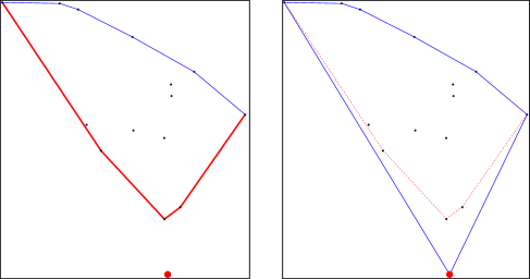
Figure 7: Incremental convex hull construction. Left: before adding the marked point, with visible faces emphasized. Right: after the addition. Note that removing the marked point from the convex hull on the right image, would result in the convex hull that appears in the left image.

Formally, these planes are defined by some normal $n$ and a point $p^{\prime}$, and have $n\cdot\left(q-p^{\prime}\right)\geq 0$ for all $q\in DP\backslash p$ but $n\cdot\left(p-p^{\prime}\right)\leq 0$. Such a plane, when translated so that its passes through $p$, is defined by $n\cdot\left(q-p\right)=0$. We note that for any $q\in DP\backslash p$, we have

$$n\cdot\left(q-p\right) = n\cdot\left(q-p+p^{\prime}-p^{\prime}\right)$$

$$= n\cdot\left(q-p^{\prime}\right)+\left(-n\cdot\left(p-p^{\prime}\right)\right)$$

$$\geq 0,$$

which means the translated plane goes through $p$, supports $\mathcal{CH}\left(DP\right)$ and has a positive $n_{z}$ component (we assumed the original face belonged to $\mathcal{LH}\left(DP\right)$). This means it satisfies the requirements of Proposition 8, and therefore this plane (translated or not) cannot be a solution to Problem 6, which concludes the proof. ∎

With regard to the computational cost of these purgings, we note that they are highly-parallelizable, in addition to being a single-pass over the points.

References

- Bronstein et al. [2006] Alexander M. Bronstein, Michael M. Bronstein, and Ron Kimmel. Generalized multidimensional scaling: a framework for isometry-invariant partial surface matching. Proc. National Academy of Sciences (PNAS), Volume 103/5:1168–1172, January 2006.
- de Berg [2000] Mark de Berg. Computational geometry: algorithms and applications. Springer, 2000. ISBN 9783540656203. URL http://books.google.com/books?id=C8zaAWuOIOcC.
- Fischer et al. [2011] Kaspar Fischer, Bernd Gärtner, Sven Schönherr, and Frans Wessendorp. Linear and quadratic programming solver. In CGAL User and Reference Manual. CGAL Editorial Board, 3.8 edition, 2011. http //www.cgal.org/Manual/3.8/doc_html/cgal_manual/packages.html#Pkg QPSolver.
- Hough [1962] Paul V. C. Hough. Method and means for recognizing complex patterns, March 1962. URL http://www.google.com/patents?vid=3069654.
- Megiddo [1984] Nimrod Megiddo. Linear programming in linear time when the dimension is fixed. Journal of The ACM, 31:114–127, 1984. doi: 10.1145/2422.322418.