Stability of Fractional Order Switching Systems

Abstract

This paper addresses the stabilization issue for fractional order switching systems. Common Lyapunov method is generalized for fractional order systems and frequency domain stability equivalent to this method is proposed to prove the quadratic stability. Some examples are given to show the applicability and effectiveness of the proposed theory.

, ,

1 Introduction

The past decade has witnessed an enormous interest in switched systems whose behaviour can be described mathematically using a mixture of logic based switching and difference/differential equations. By a switched system we mean a hybrid dynamical system consisting of a family of continuous-time subsystems and a rule that orchestrates the switching among them (Liberzon (2003), Daafouz et al. (2002)). A primary motivation for studying such systems came partly from the fact that switched systems and switched multi-controller systems have numerous applications in control of mechanical systems, process control, automotive industry, power systems, traffic control, and so on. In addition, there exists a large class of nonlinear systems which can be stabilized by switching control schemes, but cannot be stabilized by any continuous static state feedback control law Lin and Antsaklis (2009).

Recent efforts in switched system research typically focus on the analysis of dynamic behaviors, such as stability, controllability and observability, and aim to design controllers with guaranteed stability and optimized performance (refer to Lin and Antsaklis (2009), Shorten et al. (2007) for a survey in recent results in the field). To be more precise, the study of the stability issues of switched systems gives rise to a number of interesting and challenging mathematical problems, which have been of increasing interest in the recent decade.

Typically, the approach adopted to analyze these systems is to employ theories that have been developed for differential equations. To this respect, most results are based on Lyapunov’s stability theory which has played a dominant role in the analysis of dynamical systems for more than a century. Existence of quadratic Lyapunov functions for each of the constituent LTI systems is not sufficient for the stability of switched systems. However, it is well known that the switched system is stable if there exists some common Lyapunov function that satisfies the conditions of the Lyapunov theory simultaneously for all constituent subsystems (see e.g. Liberzon (2003); Narendra and Balakrishnan (1994); Mori et al. (1998); Shim et al. (1998). Although Molchanov and Pyatnitskii (1989) established a number of converse theorems, showing that such common Lyapunov function always exists when the switched linear system is stable for arbitrary switching, general conditions for determining the existence of a common Lyapunov function for switched systems are unknown. Likewise, a frequency domain method equivalent to the common Lyapunov one may make the control and stability analysis easier. For example, Kunze and Karimi (2011) propose a frequency domain equivalent of common Lyapunov function based on strictly positive realness (SPR) of the system in order to analyze the quadratic stability of switching systems.

Given this context, the contribution of our work is to bring together theories from several areas of control and to present stability issues in a unified manner for fractional order switching systems.

The remainder of this paper is organized as follows. Section 2 provides a collection of important issues concerning stability of switched systems. The main contribution of this paper is presented in Section 3, i.e., the stability theory developed for fractional order switched systems. Section 4 gives some examples to show the applicability and goodness of the proposed stability issues. Section 5 draws the concluding remarks.

2 Preliminaries

When a system becomes unstable, the output of the system goes to infinity (or negative infinity), which often poses a security problem in the immediate vicinity. Also, systems which become unstable often incur a certain amount of physical damage, which can become costly. For the sake of clarity, a collection of important issues concerning stability of switched systems is given in this section, mainly using Lyapunov theory.

2.1 Stability theorems and basic definitions

The idea behind Lyapunov’s stability theory is as follows: assume there exists a positive definite function with a unique minimum at the equilibrium. One can think of such a function as a generalized description of the energy of the system. If we perturb the state from its equilibrium, the energy will initially rise. If the energy of the system constantly decreases along the solution of the autonomous system, it will eventually bring the state back to the equilibrium. Such functions are called Lyapunov functions. While Lyapunov theorems generalize to nonlinear systems and locally stable equilibria we shall only state them in the form applicable to our system class. Consider an autonomous nonlinear dynamical system

$$\dot{x}\left(t\right)=f(x\left(t\right)),\ x\left(0\right)=x_{0},$$ (1)

where $x(t)\in\mathcal{D}\subseteq\mathbb{R}^{n}$ denotes the system state vector, $\mathcal{D}$ an open set containing the origin, and $f:\mathcal{D}\rightarrow\mathbb{R}^{n}$ continuous on $\mathcal{D}$. Suppose $f$ has an equilibrium; without loss of generality, we may assume that it is at origin. Then, Lyapunov stability for continuos systems can be summarized in the following theorems.

Theorem 1

Let $x=0$ be an equilibrium point of (1). Assume that there exists an open set $\mathcal{D}$ with $0\in\mathcal{D}$ and a continuously differentiable function $V:\mathcal{D}\rightarrow\mathbb{R}$ such that:

1. $V(0)=0,$

2. $V(x)>0$ for all $x\in\mathcal{D}\backslash\{0\}$, and

3. $\frac{\partial V}{\partial x}(x)f(x)\leq 0$ for all $x\in\mathcal{D}.$

then $x=0$ is a stable equilibrium point of (1).

Theorem 2

If, in addition, $\frac{\partial V}{\partial x}(x)f(x)\leq 0$ for all $x\in\mathcal{D}\backslash\{0\}$, then $x=0$ is an asymptotically stable equilibrium point.

Definition 1 (Quadratic Stability)

A linear system

$$\dot{x}=Ax,$$ (2)

is said to be quadratically stable in $\mathbb{R}$ if there exists a positive definite matrix $P\in\mathbb{R}^{n\times n}$ such that,

$$A^{T}P+PA<0.$$

Definition 2 ($t^{-a}$ Stability)

The trajectory $x(t)=0$ of the system $\frac{d^{\alpha}x(t)}{dt^{\alpha}}=f(t,x(t))$ is $t^{-a}$ asymptotically stable if the uniform asymptotic stability condition is met and if there is a positive real $a$ such that :
$\forall\left\|x\left(t\right)\right\|,t\leq t_{0}\ \exists\ N\left(x\left(t\right),t\leq t_{0}\right),\ t_{1}\left(x\left(t\right),t\leq t_{0}\right)$ such that $\forall t\leq t_{0},\ \left\|x\left(t\right)\right\|\leq\ N\left(t-t_{1}\right)^{-a}.$

$t^{-a}$ stability will thus be used to refer to the asymptotic stability of fractional systems. The fact that the components of the state $x(t)$ decay slowly towards $0$ following $t^{-a}$ leads to fractional systems sometimes being treated as long memory systems.

Let us consider a fractional order linear time invariant (FO-LTI) system as:

$$D^{\alpha}x=Ax,x\in\mathbb{R}^{n}$$ (3)

where $\alpha$ is the fractional order.

Theorem 3 (Moze et al. (2007))

A fractional system given by (3) with order $\alpha$, $1\leq\alpha<2$, is $t^{-a}$ asymptotically stable if and only if there exists a matrix $P=P^{T}>0$, $P\in\mathbb{R}^{n\times n}$, such that

$$\begin{bmatrix}\left(A^{T}P+PA\right)\sin\left(\phi\right)&\left(A^{T}P-PA\right)\cos\left(\phi\right)\\ \left(-A^{T}P+PA\right)\cos\left(\phi\right)&\left(A^{T}P+PA\right)\sin\left(\phi\right)\end{bmatrix}<0,$$ (4)

where $\phi=\frac{\alpha\pi}{2}$.

Theorem 4 (Moze et al. (2007))

A fractional order system given by (3) with order $\alpha$, $0<\alpha\leq 1$, is $t^{-a}$ asymptotically stable if and only if there exists a positive definite matrix $P\in\mathbb{R}^{n}$ such that

$$\left(-\left(-A\right)^{\frac{1}{2-\alpha}}\right)^{T}P+P\left(-\left(-A\right)^{\frac{1}{2-\alpha}}\right)<0.$$ (5)

2.2 Common quadratic Lyapunov functions

Consider a switched system as follows:

$$\dot{x}=Ax,A\in co\left\{A_{1},...,A_{L}\right\},$$ (6)

where $"co"$ denotes the convex combination and $A_{i},i=1,...,L$ is the switching subsystem. According to Pardalos and Rosen (1987), (6) can be alternatively written as:

$$\dot{x}=Ax,A=\sum_{i=1}^{L}\lambda_{i}A_{i},\forall\lambda_{i}\geq 0,\sum_{i=1}^{L}\lambda_{i}=1.$$ (7)

Theorem 5 (Boyd et al. (1994))

A system given by (7) is quadratically stable if and only if there exists a matrix $P=P^{T}>0$, $P\in\mathbb{R}^{n}\times n$, such that

$$A_{i}^{T}P+PA_{i}<0,\forall i=1,...,L.$$

2.3 Quadratic stability in frequency domain

Kunze and Karimi (2011) propose an equivalent to common Lyapunov stability conditions in frequency domain. The relation between SPRness and the quadratic stability can be stated in the following theorem. For further information about the specification of state space system, refer to Section 3.

Theorem 6 (Kunze and Karimi (2011))

Consider $c_{1}(s)$ and $c_{2}(s)$, two stable polynomials of order $n$, corresponding to the systems $\dot{x}=A_{1}x$ and $\dot{x}=A_{2}x$, respectively, then the following statements are equivalent:

1. $\frac{c_{1}(s)}{c_{2}(s)}$ and $\frac{c_{2}(s)}{c_{1}(s)}$ are SPR.

2. $\left|\arg(c_{1}(j\omega))-\arg(c_{2}(j\omega))\right|<\frac{\pi}{2}$ $\forall$ $\omega$.

3. $A_{1}$ and $A_{2}$ are quadratically stable, which means that $\exists P=P^{T}>0\in\mathbb{R}^{n\times n}$ such that $A_{1}^{T}P+PA_{1}<0$ , $A_{2}^{T}P+PA_{2}<0$.

3 Quadratic stability of fractional order switching systems

This section will study two ways to obtain the quadratic stability of fractional order switching systems generalizing common Lyapunov functions for fractional order switching systems and obtaining an equivalent in frequency domain, respectively.

3.1 Common quadratic Lyapunov functions of fractional order system

Let us consider a fractional order switched system as:

$$D^{\alpha}{x}=Ax,A\in co\left\{A_{1},...,A_{L}\right\},$$ (8)

where $\alpha$ is the fractional order.

Theorem 7

A fractional system described by (8) with order $\alpha$, $1\leq\alpha<2$, is quadratically stable if and only if there exists a matrix $P=P^{T}>0$, $P\in\mathbb{R}^{n\times n}$, such that

$$\begin{bmatrix}\left(A_{i}^{T}P+PA_{i}\right)\sin\left(\phi\right)&\left(A_{i}^{T}P-PA_{i}\right)\cos\left(\phi\right)\\ \left(-A_{i}^{T}P+PA_{i}\right)\cos\left(\phi\right)&\left(A_{i}^{T}P+PA_{i}\right)\sin\left(\phi\right)\end{bmatrix}<0,$$

$$\forall i=1,...,L.$$ (9)

Proof 1

System (8) can be rewritten as:

$$D^{\alpha}{x}=Ax,A=\sum_{i=1}^{L}\lambda_{i}A_{i},\forall\lambda_{i}\geq 0,\sum_{i=1}^{L}\lambda_{i}=1.$$ (10)

Then, from Theorem 3, and (8), we have

$$\begin{bmatrix}\left(\mathcal{M}^{T}P+P\mathcal{M}\right)\sin(\phi)&\left(\mathcal{M}^{T}P-P\mathcal{M}\right)\cos(\phi)\\ \left(-\mathcal{M}^{T}P+P\mathcal{M}\right)\cos(\phi)&\left(\mathcal{M}^{T}P+P\mathcal{M}\right)\sin(\phi)\end{bmatrix},$$

$$\forall\lambda_{i}\geq 0,\sum_{i=1}^{L}\lambda_{i}=1$$

$$\Leftrightarrow\sum_{i=1}^{L}\lambda_{i}\left(\begin{bmatrix}\left(A_{i}^{T}P+PA_{i}\right)\sin(\phi)&\left(A_{i}^{T}P-PA_{i}\right)\cos(\phi)\\ \left(-A_{i}^{T}P+PA_{i}\right)\cos(\phi)&\left(A_{i}^{T}P+PA_{i}\right)\sin(\phi)\end{bmatrix}\right),$$

$$\forall\lambda_{i}\geq 0,\sum_{i=1}^{L}\lambda_{i}=1.$$

where $\mathcal{M}=\sum_{i=1}^{L}\lambda_{i}A_{i}$ and $\phi=\frac{\alpha\pi}{2}$. Therefore, it is obvious that (8) is quadratically stable if and only if

$$\begin{bmatrix}\left(A_{i}^{T}P+PA_{i}\right)\sin(\phi)&\left(A_{i}^{T}P-PA_{i}\right)\cos(\phi)\\ \left(-A_{i}^{T}P+PA_{i}\right)\cos(\phi)&\left(A_{i}^{T}P+PA_{i}\right)\sin(\phi)\end{bmatrix}<0,$$

$$\forall i=1,...,L.$$ (11)

Theorem 8

A fractional system given by (8) with order $\alpha$, $0<\alpha\leq 1$, is quadratically stable if and only if there exists a matrix $P=P^{T}>0$, $P\in\mathbb{R}^{n\times n}$, such that

$$\left(-\left(-A_{i}\right)^{\frac{1}{2-\alpha}}\right)^{T}P+P\left(-\left(-A_{i}\right)^{\frac{1}{2-\alpha}}\right)<0,\forall i=1,...,L.$$ (12)

Proof 2

Assume $\left[I^{(1-\alpha)}x(t)\right]_{t=0}=0$, the fractional order system (8) with order $\alpha$, $0<\alpha\leq 1$, can be replaced by the following integer order system Moze et al. (2007):

$$\dot{z}=A_{f}z,A_{f}\in Co\left\{A_{f_{1}},...,A_{f_{L}}\right\}$$ (13)

$$z=C_{f}x,$$ (14)

where $A_{f_{i}}=\begin{bmatrix}0&\cdots&0&A_{i}^{1/\alpha}\\ A_{i}^{1/\alpha}&\cdots&0&0\\ &\ddots&&\vdots\\ \cdots&0&A_{i}^{1/\alpha}&0\end{bmatrix}$ and $C_{f}=\begin{bmatrix}0&\cdots&0&1\end{bmatrix}$. Writing (13) in an alternative way yields:

$$\dot{z}=A_{f}z,A_{f}=\sum_{i=1}^{L}\lambda_{i}A_{f_{i}},\forall\lambda_{i}\geq 0,\sum_{i=1}^{L}\lambda_{i}=1.$$ (15)

Therefore, assuming a positive definite matrix $\mathcal{P}>0$ with proper size and, based on LMI method, the system (8) with order $\alpha$, $0<\alpha\leq 1$, is quadratically stable if:

$$A^{T}_{f}\mathcal{P}+\mathcal{P}A_{f}<0\Rightarrow$$ (16)

$$\sum_{i=1}^{L}\lambda_{i}(A^{T}_{f_{i}}\mathcal{P}+\mathcal{P}A_{f_{i}})<0\Rightarrow$$ (17)

$$A^{T}_{f_{i}}\mathcal{P}+\mathcal{P}A_{f_{i}}<0,\forall i=1,...,L.$$ (18)

Then, it is obvious that expression (18) is satisfied if and only if (Moze et al. (2007))

$$(A^{1/\alpha}_{i})^{T}{P}+{P}A^{1/\alpha}_{i}<0,\forall i=1,...,L,$$ (19)

where $P$ is a positive definite matrix. In Moze et al. (2007) it is shown that condition (19) is sufficient but not necessary to guarantee quadratic stability. The necessary and sufficient condition for fractional order system is given by Theorem 5. Therefore, the necessary and sufficient condition for fractional order system is

$$\left(-\left(-A_{i}\right)^{\frac{1}{2-\alpha}}\right)^{T}P+P\left(-\left(-A_{i}\right)^{\frac{1}{2-\alpha}}\right)<0,\forall i=1,...,L.$$ (20)

3.2 Frequency domain stability

In this section, a link between quadratic stability using Lyapunov theory and SPR properties will be provided, i.e., a connection between time domain and frequency domain conditions in order to obtain quadratic stability of fractional order switching systems.

Consider a stable pseudo-polynomial of order $n\alpha$ as:

$$d(s)=s^{n\alpha}+d_{n-1}s^{(n-1)\alpha}+\cdots+d_{1}s^{\alpha}+d_{0},$$ (21)

which corresponds to the fractional order system $D^{\alpha}x=Ax$. Furthermore, consider a polynomial of order $2n$ as:

$$c(s)=s^{n}+c_{n-1}s^{(n-1)}+\cdots+c_{1}s+c_{0},$$ (22)

which corresponds to $\dot{\tilde{x}}=\tilde{A}\tilde{x}$. Assign

$$C=\begin{bmatrix}c_{2n-1},&...,&c_{1},&c_{0}\end{bmatrix},$$ (23)

$$D=\begin{bmatrix}d_{n-1},&...,&d_{1},&d_{0}\end{bmatrix}.$$ (24)

and

$$\tilde{A}=\begin{bmatrix}-c_{n-1}&-c_{n-2}&\cdots&-c_{1}&-c_{0}\\ 1&0&\cdots&0&0\\ 0&1&\cdots&0&0\\ \vdots&\vdots&\ddots&\vdots&\vdots\\ 0&0&\cdots&0&1\\ &&&&\end{bmatrix},$$ (25)

$$A=\begin{bmatrix}-d_{n-1}&-d_{n-2}&\cdots&-d_{1}&-d_{0}\\ 1&0&\cdots&0&0\\ 0&1&\cdots&0&0\\ \vdots&\vdots&\ddots&\vdots&\vdots\\ 0&0&\cdots&0&1\\ &&&&\end{bmatrix}.$$ (26)

In the following, the necessary and sufficient condition for the quadratic stability of fractional order switching systems will be given.

Theorem 9

Consider $d_{1}(s)$ and $d_{2}(s)$, two stable pseudo-polynomials of order $n$, corresponding to the systems $D^{\alpha}x=A_{1}x$ and $D^{\alpha}x=A_{2}x$ with order $\alpha$, $1\leq\alpha<2$, respectively, then the following statements are equivalent:

1. $$\left|\arg\left(\det((A_{1}^{2}-\omega^{2}I)-2(j\omega)A_{1}\sin\frac{\alpha\pi}{2})\right)-\right.$$

   $$\left.\arg\left(\det((A_{2}^{2}-\omega^{2}I)-2(j\omega)A_{2}\sin\frac{\alpha\pi}{2})\right)\right|<\frac{\pi}{2},\forall\omega.$$

2. $A_{1}$ and $A_{2}$ are quadratically stable meaning that: $\exists P=P^{T}>0\in\mathbb{R}^{n\times n}$ such that

   $$\begin{bmatrix}\left(A_{i}^{T}P+PA_{i}\right)\sin(\phi)&\left(A_{i}^{T}P-PA_{i}\right)\cos(\phi)\\ \left(-A_{i}^{T}P+PA_{i}\right)\cos(\phi)&\left(A_{i}^{T}P+PA_{i}\right)\sin(\phi)\end{bmatrix}<0,$$

   $$\forall i=1,2.$$

Proof 3

Consider $c_{1}(s)$ and $c_{2}(s)$ are characteristic polynomials corresponding to $\dot{\tilde{x}}=\tilde{A}_{1}\tilde{x}$ and $\dot{\tilde{x}}=\tilde{A}_{2}\tilde{x}$, respectively, where $\tilde{A}_{i}=\begin{bmatrix}A_{i}\sin(\phi)&A_{i}\cos(\phi)\\ -A_{i}\cos(\phi)&A_{i}\sin(\phi)\end{bmatrix},i=1,2.$ According to Theorem 6, the following statements are equivalents:

1. $\frac{c_{1}(s)}{c_{2}(s)}$ and $\frac{c_{2}(s)}{c_{1}(s)}$ are SPR, where $c_{i}(s)=\det(sI-\tilde{A}_{i}),i=1,2$.

2. $\left|\arg(c_{1}(j\omega))-\arg(c_{2}(j\omega))\right|<\frac{\pi}{2}$ $\forall$ $\omega$.

3. $\tilde{A}_{1}$ and $\tilde{A}_{2}$ are quadratically stable meaning that: $\exists\mathcal{P}=\mathcal{P}^{T}>0\in\mathbb{R}^{2n\times 2n}$ such that $\tilde{A}_{1}^{T}\mathcal{P}+\mathcal{P}\tilde{A}_{1}<0$ , $\tilde{A}_{2}^{T}\mathcal{P}+\mathcal{P}\tilde{A}_{2}<0$.

Now, consider $d_{1}(s)$ and $d_{2}(s)$ are characteristic pseudo-polynomials corresponding to the fractional order systems $D^{\alpha}x=A_{1}x$ and $D^{\alpha}x=A_{2}x$ with order $\alpha$, $1\leq\alpha<2$, respectively. The relation between $A_{i}$ and $\tilde{A}_{i}$ is given by (25). From (22), we have

$$\left|\arg(c_{1}(j\omega))-\arg(c_{2}(j\omega))\right|=$$

$$\left|\arg(j\omega I-\tilde{A_{1}})-\arg(j\omega I-\tilde{A_{2}})\right|<\frac{\pi}{2},$$

$$\Leftrightarrow\left|\arg\left(\det((A_{1}^{2}-\omega^{2}I)-2(j\omega)A_{1}\sin(\phi)\right)-\right.$$

$$\left.\arg\left(\det((A_{2}^{2}-\omega^{2}I)-2(j\omega)A_{2}\sin(\phi)\right)\right|<\frac{\pi}{2},\forall\omega.$$

where $I$ is the identity matrix with the proper size.

Define, $\mathcal{P}=\begin{bmatrix}P&0\\ 0&P\end{bmatrix},P=P^{T}>0,P\in\mathbb{R}^{n\times n}$. Then,

$$\tilde{A}_{i}^{T}\mathcal{P}+\mathcal{P}\tilde{A}_{i}=\begin{bmatrix}A_{i}^{T}\sin(\phi)&-A_{i}^{T}\cos(\phi)\\ A_{i}^{T}\cos(\phi)&A_{i}^{T}\sin(\phi)\end{bmatrix}\begin{bmatrix}P&0\\ 0&P\end{bmatrix}+$$

$$\begin{bmatrix}P&0\\ 0&P\end{bmatrix}\begin{bmatrix}A\sin(\phi)&A\cos(\phi)\\ -A\cos(\phi)&A\sin(\phi)\end{bmatrix}<0,$$

$$\Leftrightarrow\begin{bmatrix}\left(A_{i}^{T}P+PA_{i}\right)\sin(\phi)&\left(A_{i}^{T}P-PA_{i}\right)\cos(\phi)\\ \left(-A_{i}^{T}P+PA_{i}\right)\cos(\phi)&\left(A_{i}^{T}P+PA_{i}\right)\sin(\phi)\end{bmatrix}<0,$$

$$\forall i=1,2.$$

Therefore, the theorem is proved.

Theorem 10

Consider two stable fractional order systems $D^{\alpha}x=A_{1}x$ and $D^{\alpha}x=A_{2}x$ with order $\alpha$, $0<\alpha\leq 1$, then the following statements are equivalent:

1. $\left|\arg(\det(\mathcal{A}_{1}-j\omega I))-\arg(\det(\mathcal{A}_{2}-j\omega I))\right|<\frac{\pi}{2}$ $\forall$ $\omega$.

2. $A_{1}$ and $A_{2}$ are quadratically stable, which means that $\exists P=P^{T}>0\in\mathbb{R}^{n\times n}$ such that

   $$\left(-\left(-A_{i}\right)^{\frac{1}{2-\alpha}}\right)^{T}P+P\left(-\left(-A_{i}\right)^{\frac{1}{2-\alpha}}\right)<0,\forall i=1,2,$$

where $\mathcal{A}_{i}=-\left(-A_{i}\right)^{\frac{1}{2-\alpha}},\forall i=1,2$ and $I$ is the identity matrix.

Proof 4

Define $c_{i}(s)=\det(\mathcal{A}_{i}-sI)$, $i=1,2$. According to Theorem 6 and common quadratic stability theorem for fractional order system with order $\alpha$, $0<\alpha\leq 1$, i.e., Theorem 12, proof is straightforward.

Although the theory developed in the frequency domain no necessarily proves the SPRness, a relation was obtained as an equivalent issue of quadratic stability. Concerning the ease of designing fractional order controllers in frequency domain, the stability analysis in frequency domain will be really useful for fractional order switching systems.

4 Illustrative Examples

In this section, some examples are given in order to show the applicability of the theories developed for fractional order switching systems.

Example 1

Let us consider the switching system (8) with order $\alpha=0.6$, where $A_{1}=\begin{bmatrix}0.3529&1.6044\\ -1.6044&-4.4602\end{bmatrix}$ and $A_{2}=\begin{bmatrix}0.3661&0.9237\\ -0.4618&-0.1558\end{bmatrix}$. Applying Theorem 12 yields:

$$\mathcal{A}_{1}=\begin{bmatrix}0&1\\ -1&-3\end{bmatrix},\mathcal{A}_{2}=\begin{bmatrix}0&1\\ -0.5&-0.5\end{bmatrix}$$

Then, choosing a common matrix $P=\begin{bmatrix}3&1\\ 1&4\end{bmatrix}$, the stability conditions

$$\left(-\left(-A_{1}\right)^{\frac{1}{2-\alpha}}\right)^{T}P+P\left(-\left(-A_{1}\right)^{\frac{1}{2-\alpha}}\right)=\begin{bmatrix}-2&-4\\ -4&-22\end{bmatrix}<0$$

$$\left(-\left(-A_{2}\right)^{\frac{1}{2-\alpha}}\right)^{T}P+P\left(-\left(-A_{2}\right)^{\frac{1}{2-\alpha}}\right)=\begin{bmatrix}-1&0.5\\ 0.5&-2\end{bmatrix}<0$$

are satisfied and the switching system is quadratically stable. Now let us compare the results with the frequency domain analysis. Applying Theorem 10, the following condition

$$\left|\tan^{-1}\left(\frac{3\omega}{1+\omega^{2}}\right)-\tan^{-1}\left(\frac{0.5\omega}{0.5+\omega^{2}}\right)\right|<\frac{\pi}{2},\forall\omega$$ (27)

should be satisfied. The phase difference of (27) is depicted in Fig. 1. As can be observed, the maximum phase difference is $51.51^{o}$, which is less than $90^{o}$, that implies the switching stability condition is satisfied and the system is quadratically stable.

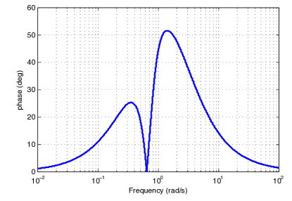
Figure 1: Phase difference of condition (27) for the system in Example 1

Example 2

Now, let us consider the switching system given by (8) with order $\alpha=0.75$, where $A_{1}=\begin{bmatrix}0&1\\ -1&0.5\end{bmatrix}$ and $A_{2}=\begin{bmatrix}0&1\\ -0.5&0.1\end{bmatrix}$. Applying Theorem 10, we have:

$$\mathcal{A}_{1}=\begin{bmatrix}-0.3684&1.0263\\ -1.0263&0.1448\end{bmatrix},\mathcal{A}_{2}=\begin{bmatrix}-0.2450&1.0390\\ -0.5195&-0.1411\end{bmatrix}$$

and the following frequency domain condition

$$\left|\tan^{-1}\left(\frac{0.2236\omega}{1+\omega^{2}}\right)-\tan^{-1}\left(\frac{0.3861\omega}{0.4977+\omega^{2}}\right)\right|<\frac{\pi}{2},\forall\omega$$ (28)

should be satisfied. The same as previous example, condition (28) is depicted in Fig. 2. It is shown that the maximum phase difference of condition (28) is $80.02^{o}$, so the switching system is quadratically stable.

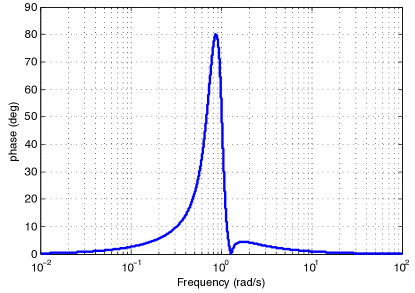
Figure 2: Phase difference of condition (28) for the system in Example 2

Example 3

Let us now consider the same switching system as in Example 2, but with an order bigger than $1$, $1<\alpha<2$. Applying Theorem 9, the following condition:

$$\left|\arg\left(\det\left(\begin{bmatrix}-1.75-\omega^{2}&-2.1-2j\sin(\phi)\\ 3.675+3.5j\sin(\phi)&2.66-\omega^{2}+4.2j\sin(\phi)\end{bmatrix}\right)\right)-\right.$$

$$\left.\arg\left(\det\left(\begin{bmatrix}-3-\omega^{2}&-3-2j\sin(\phi)\\ 9+6j\sin(\phi)&6-\omega^{2}+6j\sin(\phi)\end{bmatrix}\right)\right)\right|<\frac{\pi}{2},\forall\omega$$ (29)

where $\phi=\frac{\alpha\pi}{2}$ should be satisfied for all $\alpha$, $1<\alpha<2$. Figure 3 represents the condition (29) when the fractional order $\alpha$ is changing in the interval $(1,2)$. In order to make this example clearer, the interval of variation of $\alpha$ is divided into three subintervals. As a matter of fact, Fig. 3 (a) shows the phase difference (29) for systems with the order $\alpha\in(1,1.5]\cup[1.7,2)$, whereas Fig. 3 (b) corresponds to systems with order $\alpha\in(1.5,1.7)$. As can be seen, the system is quadratically stable if its order $\alpha\in(1,1.5]\cup[1.7,2)$. The stability region of the considered system is shown in Fig. 4, in which the maximum values of (29) are plotted versus its order $\alpha$.

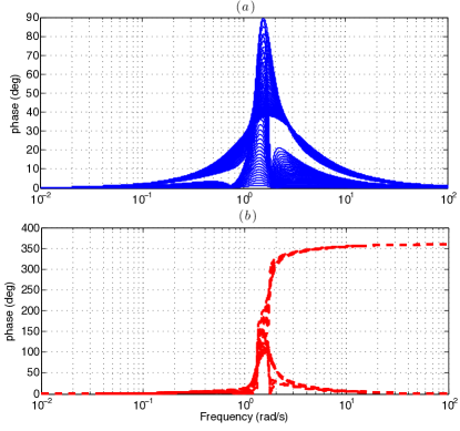
Figure 3: Phase difference of condition (29) for the system in Example 3 for different values of the order $\alpha$: (a) $\alpha\in(1,1.5]\cup[1.7,2)$ (b) $\alpha\in(1.5,1.7)$

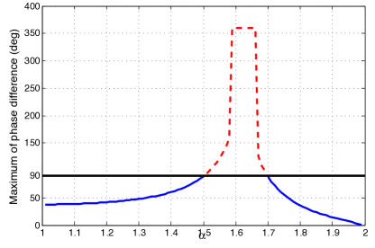
Figure 4: Maximum value of (29) versus $\alpha$

5 Conclusion

This paper studies the quadratic stability for fractional order switching systems. In particular, equivalent Lyapunov conditions in frequency domain are developed for this kind of systems to prove their quadratic stability. Some illustrative examples are given to show the applicability and validation of the proposed theory.

Our future efforts will focus on finding a relation between the frequency domain method proposed in this paper and SPRness.

References

Boyd et al. [1994]
Boyd, S., Ghaoui, L.E., Feron, E., and Balakrishnan, V. (1994).
Linear Matrix Inequalities in System and Control Theory.
SIAM.
Daafouz et al. [2002]
Daafouz, J., Riedinger, P., and Iung, C. (2002).
Stability analysis and control synthesis for switched systems: A
switched Lyapunov function approach.
IEEE Transactions on Automatic Control, 47(11), 1883 – 1887.