1INFN, Laboratori Nazionali di Frascati,
Via E. Fermi 40, I-00044, Frascati,
Italy
2Dipartimento di Fisica, Università di Roma ’La Sapienza’
and INFN, Sezione di Roma,
Piazzale A. Moro 2, I-00185, Roma, Italy
Searching for heavy neutral gauge bosons , predicted in extensions of the Standard Model based on a gauge symmetry, is one of the challenging objectives of the experiments carried out at the Large Hadron Collider. In this paper, we study phenomenology at hadron colliders according to several -based models and in the Sequential Standard Model. In particular, possible decays into supersymmetric particles are included, in addition to the Standard Model modes so far investigated. We point out the impact of the group on the MSSM spectrum and, for a better understanding, we consider a few benchmarks points in the parameter space. We account for the D-term contribution, due to the breaking of , to slepton and squark masses and investigate its effect on decays into sfermions. Results on branching ratios and cross sections are presented, as a function of the MSSM and parameters, which are varied within suitable ranges. We pay special attention to final states with leptons and missing energy and make predictions on the number of events with sparticle production in decays, for a few values of integrated luminosity and centre-of-mass energy of the LHC.
Keywords: Physics Beyond the Standard Model; Collider
Phenomenology;
Supersymmetry;
Heavy Gauge Bosons; Grand Unification Theories.
1 Introduction
The Standard Model (SM) of the strong and electroweak interactions has been so far successfully tested at several machines, such the LEP and Tevatron accelerators and has been lately confirmed by the data collected by the Large Hadron Collider (LHC). New physics models have nonetheless been proposed to solve the drawbacks of the SM, namely the hierarchy problem, the Dark Matter observation or the still undetected Higgs boson, responsible for the mass generation. The large amount of data collected at the centre-of-mass energy of 7 TeV at the LHC opens a window to extensively search for new physics. The further increase to 8 and ultimately 14 TeV, as well as higher integrated luminosities, will extend this investigation in the near future.
The simplest possible extension of the SM consists in a gauge group of larger rank involving the introduction of one extra factor, inspired by Grand Unification Theories (GUTs), which leads to the prediction of a new neutral gauge boson . The phenomenology of the has been studied from a theoretical viewpoint (see, e.g., the reviews [1, 2] or the more recent work in Refs. [3, 4]), whereas searches for new heavy gauge bosons have been carried out at the Tevatron by the CDF [5] and D0 [6] Collaborations and at the LHC by ATLAS [7] and CMS [8]. Besides the bosons yielded by the extra group, the analyses have also investigated the so-called Sequential Standard Model (), i.e. a with the same couplings to fermions and gauge bosons as the of the SM. The Sequential Standard Model does not have theoretical bases like the models, but it is used as a benchmark, since, as will be seen later on, the production cross section is just function of the mass and there is no dependence on other parameters.
The Tevatron analyses searched for high-mass dielectron resonances in collisions at 1.96 TeV and set a lower mass limit of about 1023 (D0) and 963 (CDF) GeV for the . The LHC experiments investigated the production of both dielectrons and dimuons at large invariant masses and several models of production, i.e. different gauge groups. The CMS Collaboration, by using event samples corresponding to an integrated luminosity of fb-1, excluded a with SM-like couplings and mass below 2.32 TeV, a GUT-inspired below 1.49-1.69 TeV and a Kaluza–Klein graviton in extra-dimension models [9] below 0.71-1.63 TeV. The ATLAS Collaboration analyzed 5 fb-1 of data and obtained a bound of 2.21 TeV for the SM-like case, in the range 1.76-1.96 TeV for the scenarios and about 0.91-2.16 TeV for the Randall–Sundrum gravitons 111The exclusion ranges depend on the specific model and, for the graviton searches, on the coupling value..
All such analyses, and therefore the obtained exclusion limits, crucially rely on the assumption that the decays into Standard Model particles, with branching ratios depending on its mass and, in the GUT-driven case, on the parameters characterizing the specific model: such a choice is dictated by the sake of minimizing the parameters ruling the phenomenology. As a matter of fact, in the perspective of searching for new physics at the LHC, there is no actual reason to exclude decays into channels beyond the SM, such as its supersymmetry. In fact, new physics contributions to the width will significantly decrease the branching ratios into SM particles, and therefore the mass limits quoted by the experiments may have to be revisited. Furthermore, decays into supersymmetric particles, if existing, represent an excellent tool to investigate the electroweak interactions at the LHC in a phase-space corner that cannot be explored by employing the usual techniques. Therefore, the possible discovery of supersymmetry in processes would open the road to additional investigations, since one would need to formulate a scenario accommodating both sparticles and heavy gauge bosons.
The scope of this paper is indeed the investigation of the phenomenology of bosons at the LHC, assuming that they can decay into both SM and supersymmetric particles. As for supersymmetry, we shall refer to the Minimal Supersymmetric Standard Model (MSSM) [10, 11] and study the dependence on the MSSM parameters. A pioneering study of supersymmetric contributions to decays was carried out in [12], wherein the partial widths in all SM and MSSM channels were derived analytically, and the branching ratios computed for a few scenarios. However, the numerical analysis was performed for a mass =700 GeV, presently ruled out by the late experimental measurements, and only for one point of the supersymmetric phase space. Therefore, no firm conclusion could be drawn about the feasibility to search for the within supersymmetry at the LHC. This issue was tackled again more recently. Ref. [13] studied how the mass exclusion limits change once sparticle and exotic decay modes are included, for many models and varying the supersymmetric particle masses from 0 to 2.5 TeV. The Higgs and neutralino sectors in extensions of the MSSM, including GUT-inspired models, were thoroughly debated in [14] and [15], respectively. Ref. [16] considered the B-L gauge group, B and L being the baryon and lepton numbers, and focused on the decay of the into charged-slepton pairs for a few points in the MSSM phase space and various values of and slepton masses. Ref. [17] investigated all possible decays of the in the SM and MSSM, and several models, for two sets of supersymmetric parameters and a mass in the 1-2 TeV range.
In the following, we shall extend the above work in several aspects. Special attention will be paid to the MSSM spectrum after the addition of the gauge symmetry. Squark and slepton masses will be parametrized as the sum of a soft mass and the so-called D- and F-terms [18]. In particular, accounting for the D-term has an impact on the sfermion masses, which get an extra contribution driven by the group. Higgs, chargino and neutralino masses will be determined by diagonalizing the corresponding mass matrices. A detailed study will be thereafter undertaken by allowing the and MSSM parameters to run within suitable ranges, taking into account the recent experimental limits. Throughout this work, particular care will be taken about the decay of the into slepton pairs, i.e. charged sleptons or sneutrinos, eventually leading to final states with four charged leptons or two charged leptons and missing energy, due to neutralinos. In fact, in the complex hadronic environment of the LHC, leptonic final states are the best channels to perform precise measurements and searches. Slepton production in decays has the advantage that the mass is a further kinematical constrain on the invariant mass of the slepton pair. Moreover, the extension of the MSSM by means of the gauge group provides also an interesting scenario to study Dark Matter candidates, such as neutralinos [19, 20] or right-handed sneutrinos [21], whose annihilation or scattering processes may proceed through the coupling with a boson.
We shall present results for the production cross sections and the branching ratios into both Standard Model and supersymmetric final states, thoroughly scanning the U(1)′ and MSSM parameter spaces, which will enable one to estimate the LHC event rates with sparticle production in decays. We point out that, in order to draw a statement on the feasibility of the LHC to search for supersymmetry in decays, one should also account for the Standard Model backgrounds. However, in assessing whether the signal can be separated from the background, one would need to consider exclusive final states, wherein acceptance cuts on final-state jets, leptons and possible missing energy, as well as detector effects, are expected to play a role. The framework of a Monte Carlo generator [22, 23], wherein both signal and background events are provided with parton showers, hadronization, underlying event and detector simulations, is therefore the ideal one to carry out such a comparison. We shall thus defer a detailed investigation of the backgrounds to a future study, after the implementation of our modelling for production and decay in a Monte Carlo code.
The paper is organized as follows. In Section 2 we shall briefly discuss the gauge group yielding the boson and the particle content of the MSSM. Section 3 will be devoted to summarize the new features of the MSSM, once it is used in conjunction with the group. In Section 4, as a case study, we will choose a specific point of the MSSM/ parameter space, named ‘Representative Point’, and discuss the MSSM spectrum in this scenario. In Section 5, we shall present the branching ratios into SM and BSM particles for several models and in the Sequential Standard Model. We will first investigate the decay rates in a particular ‘Reference Point’ of the parameter space and then vary the mixing angle and the MSSM parameters. Particular attention will be devoted to the decays into sleptons and to the dependence of the branching fractions on the slepton mass. In Section 6 the leading-order cross section for production in the scenarios and in the Sequential Standard Model will be calculated. Besides, the number of events with sparticle production in decays will be computed for a few energy and luminosity phases of the LHC. In Section 7 we shall summarize the main results of our study and make some final remarks on the future developments of the analysis here presented. In Appendix A the main formulas used to calculate the branching ratios will be presented.
2 Modelling production and decay
As discussed in the Introduction, we shall consider extensions of the Standard Model leading to bosons, which will be allowed to decay into both SM and supersymmetric particles. For the sake of simplicity and minimizing the dependence of our analysis on unknown parameters, we shall refer to the MSSM. In this section we wish to briefly review the main aspects of the models used for production and decay.
2.1 models and charges
There are several possible extensions of the SM that can be achieved by adding an extra gauge group, typical of string-inspired GUTs (see, e.g., Refs. [1, 2] for a review): each model is characterized by the coupling constants, the breaking scale of and the scalar particle responsible for its breaking, the quantum numbers of fermions and bosons according to . Throughout our work, we shall focus on the models explored by the experimental collaborations.
Among the gauge models, special care has been taken about those coming from a Grand Unification gauge group , having rank 6, which breaks according to:
| (1) |
followed by
| (2) |
The neutral vector bosons associated with the and groups are called and , respectively. Any other model is characterized by an angle and leads to a boson which can be expressed as 222In Eq. (3) we followed the notation in [12] and we shall stick to it throughout this paper. One can easily recover the notation used in [1] by replacing .:
| (3) |
The orthogonal combination to Eq. (3) is supposed to be relevant only at the Planck scale and can therefore be neglected even at LHC energies. Another model, named U(1), is inherited by the direct breaking of to the Standard Model (SM) group, i.e. SU(2) U(1)Y, as in superstring-inspired models:
| (4) |
The yielded gauge boson is called and corresponds to a mixing angle in Eq. (3). The model orthogonal to U(1), i.e. , leads to a neutral boson which will be referred to as . Furthermore, in the so-called secluded model, a S model extends the MSSM with a singlet field [24]. The connection with the E6 groups is achieved assuming a mixing angle and a gauge boson .
In the Grand Unification group E6 the matter superfields are included in the fundamental representation of dimension 27:
| (5) |
In Eq. (5), is a doublet containing the left-handed quarks, i.e.
| (6) |
whereas includes the left-handed leptons:
| (7) |
In Eqs. (6) and (7), , and denote generic quark and lepton flavours. Likewise, , , and are singlets, which are conjugate to the left-handed fields and thus correspond to right-handed quarks and leptons 333Following [18], the conjugate fields are related to the right-handed ones via relations like .. In the case of supersymmetric extensions of the Standard Model, such as the MSSM, , , , , and will be superfields containing also left-handed sfermions. Furthermore, in Eq. (5), and are colour-singlet, electroweak doublets which can be interpreted as Higgs pairs:
| (8) |
In the MSSM, and are superfields containing also the supersymmetric partners of the Higgs bosons, i.e. the fermionic higgsinos. Another possible description of the and fields in the representation 27 is that they consist of left-handed exotic leptons (sleptons) and , with the same SM quantum numbers as the Higgs fields in Eq. (8) [12] 444In the assumption that and contain exotic leptons, it is: and .. Moreover, in Eq. (5), and are exotic vector-like quarks (squarks) and is a SM singlet 555A variety of notation is in use in the literature to denote the exotic fields in the 27 representation. For example, in [2, 25, 26] the exotic quarks and are called and .. In our phenomenological analysis, as well as in those performed in Refs. [12, 16, 17], leptons and quarks contained in the and fields are neglected and assumed to be too heavy to contribute to phenomenology. We are nevertheless aware that this is a quite strong assumption and that in forthcoming BSM investigations one may well assume that such exotics leptons and quarks (sleptons and squarks) are lighter than the and therefore they can contribute to decays.
When E6 breaks according to Eqs. (1) and (2), the fields in Eq. (5) are reorganized according to SO(10) and SU(5). The SU(5) representations are the following:
| (9) |
From the point of view of SO(10), the assignment of the fields in the representations 16, 10 and 1 is not uniquely determined. In particular, there is no actual reason to decide which representation should be included in 16 rather than in 10. The usual assignment consists in having in the representation 16 the SM fermions and in the 10 the exotics:
| (10) |
An alternative description is instead achieved by including and in the 16, with and in the 10; this ’unconventional’ E6 scenario has been intensively studied in Refs. [25, 26, 27] and leads to a different phenomenology. In our paper, we shall assume the ‘conventional’ SO(10) representations, as in Eq. (10). Nevertheless, it can be shown [27] that, given a mixing angle , the unconventional E6 scenario can be recovered by applying the transformation:
| (11) |
In fact, in our phenomenological analysis, we shall also consider the N model leading to the so-called boson, with a mixing angle . According to Eq. (11), the model corresponds to the one, but in the unconventional E6 scenario. Table 1 summarizes the -based models which will be investigated throughout this paper, along with the values of the mixing angle .
The charges of the fields in Eq. (5), assuming that they are organized in the SO(10) representations as in (10), are listed in Table 2. Under a generic rotation, the charge of a field is the following combination of the and charges:
| (12) |
| Model | |
|---|---|
| 0 | |
| -1 | 1 | |
| -1 | 1 | |
| 3 | 1 | |
| 3 | 1 | |
| -1 | 1 | |
| -5 | 1 | |
| -2 | -2 | |
| 2 | -2 | |
| 0 | 4 | |
| 2 | -2 | |
| -2 | -2 |
Besides the gauge groups, another model which is experimentally investigated is the so-called Sequential Standard Model (SSM), yielding a gauge boson , heavier than the boson, but with the same couplings to fermions and gauge bosons as in the SM. As discussed in the Introduction, although the SSM is not based on strong theoretical arguments, studying the phenomenology is very useful, since it depends only on one parameter, the mass, and therefore it can set a benchmark for the -based analyses.
In the following, the coupling constants of , and will be named , and , respectively, with , being the Weinberg angle. We shall also assume, as occurs in E6-inspired models, a proportionality relation between the two U(1) couplings, as originally proposed in [28]:
| (13) |
Before closing this subsection, we wish to stress that, in general, the electroweak-interaction eigenstates and mix to yield the mass eigenstates, usually labelled as and . Ref. [29] addressed this issue by using precise electroweak data from several experiments and concluded that the mixing angle is very small for any model, namely -. Likewise, even the mixing associated with the extra kinetic terms due to the two U(1) groups is small and can be neglected [30].
2.2 Particle content of the Minimal Supersymmetric Standard Model
The Minimal Supersymmetric Standard Model (MSSM) is the most investigated scenario for supersymmetry, as it presents a limited set of new parameters and particle content with respect to the Standard Model. Above all, the MSSM contains the supersymmetric partners of the SM particles: scalar sfermions, such as sleptons and () and squarks (), and fermionic gauginos, i.e. , , and . It exhibits two Higgs doublets, which, after giving mass to and bosons, lead to five scalar degrees of freedom, usually parametrized in terms of two CP-even neutral scalars, and , with lighter than , one CP-odd neutral pseudoscalar , and a pair of charged Higgs bosons . Each Higgs has a supersymmetric fermionic partner, named higgsino. The light scalar Higgs, i.e. , roughly corresponds to the SM Higgs.
The weak gauginos mix with the higgsinos to form the mass eigenstates: two pairs of charginos (and ) and four neutralinos (, , and ), where is the lightest and the heaviest. Particle masses and couplings in the MSSM are determined after diagonalizing the relevant mass matrices. Hereafter, we assume the conservation of R-parity, with the values = +1 for SM particles and = -1 for their supersymmetric partners. This implies the existence of a stable Lightest Supersymmetric Particle (LSP), present in any supersymmetric decay chain. The lightest neutralino, i.e. , is often assumed to be the LSP.
As for the Higgs sector, besides the two Higgs doublets of the MSSM, the extra requires another singlet Higgs to break the symmetry and give mass to the itself. Moreover, two extra neutralinos are necessary, since one has a new neutral gaugino, i.e. the supersymmetric partner of the , and a further higgsino, associated with the above extra Higgs. As for the sfermions, squark and slepton masses will get an an extra contribution to the so-called D-term, depending on the sfermion charges and Higgs vacuum expectation values. As will be discussed below, such D-terms, when summed to the soft masses and to the F-terms, will have a crucial impact on sfermion spectra and, whenever large and negative, they may even lead to discarding some MSSM/ scenarios.
3 Extending the MSSM with the extra group
In our modelling of production and decay into SM as well as supersymmetric particles, the phenomenological analysis in Ref. [12] will be further expanded and generalized. In this section we summarize a few relevant points which are important for our discussion, referring to the work in [12] for more details.
3.1 Higgs bosons in the MSSM and U models
The two Higgs doublets predicted by the MSSM ( and ) can be identified with the scalar components of the superfields and in Eq. (5), whereas the extra Higgs (), necessary to break the symmetry and give mass to the , is associated with the scalar part of the singlet . The three Higgs bosons are thus two weak-isospin doublets and one singlet:
, , .
The vacuum expectation values of the neutral Higgs bosons are given by , with . From the Higgs vacuum expectation values, one obtains the MSSM parameter , i.e.
| (14) |
Hereafter, we shall denote the Higgs charges according to the U(1)′ symmetry as:
| (15) |
Their values can be obtained using the numbers in Table 2 and Eq. (12).
The MSSM superpotential contains a Higgs coupling term giving rise to the well-known parameter; because of the extra field , our model presents the additional contribution , leading to a trilinear scalar potential for the neutral Higgs bosons
| (16) |
The parameter in Eq. (16) is related to the usual term by means of the following relation, involving the vacuum expectation value of [12]:
| (17) |
After symmetry breaking and giving mass to , and bosons, one is left with two charged (), and four neutral Higgs bosons, i.e. one pseudoscalar and three scalars , and 666We point out that in [12] the three neutral Higgs bosons are denoted by , with and the pseudoscalar one by .. Following [31], the charged-Higgs mass is obtained by diagonalizing the mass mixing matrix
| (18) |
and is given by
| (19) |
We refer to [12] for the mass matrix of the CP-even neutral Higgs bosons: the mass eigenvalues are to be evaluated numerically and cannot be expressed in closed analytical form. One can nonetheless anticipate that the mass of the heaviest is typically about the mass, and therefore the cannot decay into channels containing .
The mass of the pseudoscalar Higgs is obtained after diagonalizing its mass matrix and can be computed analytically, as done in [31]:
| (20) |
where 777In Eqs. (19) and (20) we have fixed the typing mistakes contained in Ref. [12], wherein the expressions for the masses of charged and pseudoscalar Higgs bosons contain extra factors of 2..
3.2 Neutralinos and charginos
Besides the four neutralinos of the MSSM, , two extra neutralinos are required, namely and , associated with the and with the new neutral Higgs breaking . The neutralino mass matrix is typically written in the basis of the supersymmetric neutral bosons . It depends on the Higgs vacuum expectation values, on the soft masses of the gauginos , and , named , and hereafter, and on the Higgs charges , and . It reads:
| (21) |
The neutralino mass eigenstates and their masses are obtained numerically after diagonalizing the above matrix. Approximate analytic expressions for the neutrino masses, valid whenever , , , and are much smaller than , can be found in [32].
Since the new and Higgs bosons are neutral, the chargino sector of the MSSM remains unchanged even after adding the extra group. The chargino mass matrix is given by [10]
| (22) |
and its eigenvalues are
| (23) |
with
| (24) |
3.3 Sfermions
In principle, for the sake of a reliable determination of the sfermion masses, one would need to carry out a full investigation within models for supersymmetry breaking, such as gauge-, gravity- or anomaly-mediated mechanisms. Studying supersymmetry-breaking scenarios goes nevertheless beyond the scopes of the present work. We just point out that supersymmetry can be spontaneously broken if the so-called D-term and/or the F-term in the MSSM scalar potential have non-zero vacuum expectation values, which can be achieved by means of the Fayet–Iliopoulos [33] or O’Raifeartaigh [34] mechanisms, respectively. 888The scalar potential is given, in terms of D- and F-terms, by , with and , where is the superpotential, are the scalar (Higgs) fields, and the coupling constant and the generators of the gauge group of the theory.
The sfermion squared masses can thus be expressed as the sum of a soft term , often set to the same value for both squarks and sleptons at a given scale, and the corrections due to D- and F-terms [18]. The F-terms are proportional to the SM fermion masses and therefore they are mostly relevant for the stop quarks. The D-term can be, in principle, important for both light and heavy sfermions and, for the purpose our study, it consists of two contributions. A first term is a correction due to the hyperfine splitting driven by the electroweak symmetry breaking, already present in the MSSM. For a fermion of weak isospin , weak hypercharge and electric charge , this contribution to the D-term reads:
| (25) |
A second contribution is due to possible extensions of the MSSM, such as our group, and is related to the Higgs bosons which break the new symmetry:
| (26) |
where , and are the Higgs charges defined in Eq. (15) and the charge of sfermion . When dealing with the Sequential Standard Model , only the first contribution to the D-term, Eq. (25), must be evaluated.
Left- and right-handed sfermions mix and therefore, in order to obtain the mass eigenstates, one needs to diagonalize the following squared mass matrix:
| (27) |
The value of the soft masses and the scale at which they are evaluated are in principle arbitrary, as long as the physical sfermion masses, obtained after diagonalizing the matrix (27), fall within the current experimental limits for slepton and squark searches. Following Ref. [12], we assume a common soft mass of the order of few TeV for all the sfermions at the scale and add to it the D- and F-term contributions. Another possibility would be, as done e.g. in [18], fixing the soft mass at a high ultraviolet scale, such as the Planck mass, and then evolving it down to the typical energy of the process, by means of renormalization group equations.
As an example, we present the expression for the matrix elements in the case of an up-type squark:
| (28) | |||||
| (29) | |||||
| (30) |
where , is the soft mass at the energy scale and is the coupling constant entering in the Higgs-sfermion interaction term.
The dependence on and on the mixing angle is embedded in the term; analogous expressions hold for down squarks and sleptons [12]. In the following, the up-squark mass eigenstates will be named as and and their masses as and . Likewise, , and will be the mass eigenstates for down-type squarks, charged sleptons and sneutrinos and their masses will be denoted by , and , respectively.
The terms in Eqs. (28) and (29), as well as the the mixing term (30) are inherited by the F-terms in the scalar potential. As the mass of SM light quarks and leptons is very small, such terms are typically irrelevant and the mass matrix of sleptons and light squarks is roughly diagonal. On the contrary, the mixing term can be relevant for top squarks, and therefore the stop mass eigenstates can in principle be different from the weak eigenstates . However, we can anticipate that, as will be seen later on, for a boson with a mass of the order of a few TeV, much higher than the top-quark mass, even the stop mixing term will be negligible.
4 Representative Point
The investigation on production and decays into SM and BSM particles depends on several parameters, such as the or supersymmetric particle masses; the experimental searches for physics beyond the Standard Model set exclusion limits on such quantities [35].
In the following, we shall first consider a specific configuration of the parameter space, which we call ’Representative Point’, to study the phenomenology in a scenario yielding non-zero branching ratios in the more relevant decay channels. Then, each parameter will be varied individually, in order to investigate its relevance on the physical quantities.
The set of parameters chosen is the following:
| (31) |
where the value of corresponds to the model and by and we have denoted any possible quark and lepton flavour, respectively. In Eq. (31) the gaugino masses and satisfy, within very good accuracy, the following relation, inspired by Grand Unification Theories:
| (32) |
4.1 Sfermion masses
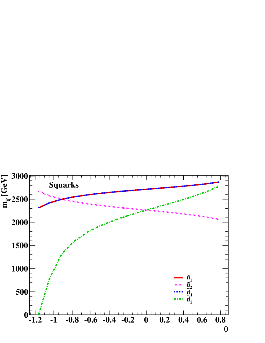
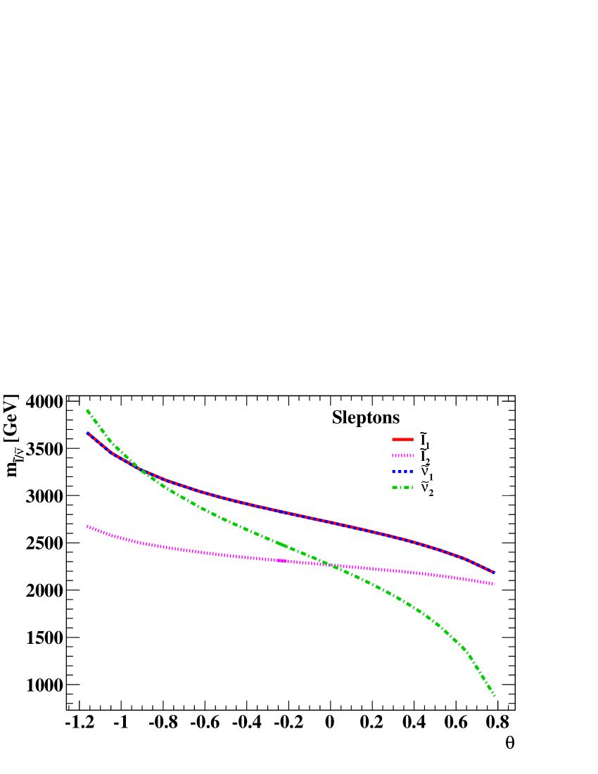
The sfermion masses are given by the sum of a common soft mass, which we have set to the same values for all squarks and sleptons at the scale, as in Eq. (31), and the F- and D-terms, given in Eqs. (27)–(30). The D-term, and then the sfermion squared masses, is expected to depend strongly on the and MSSM parameters, and can possibly be negative and large, up to the point of leading to an unphysical (imaginary) sfermion mass. The F-term, being proportional to the lepton/quark masses, is significant only for top squarks. In Fig. 1 we study the dependence of squark (left) and slepton (right) masses on the mixing angle . The symbols , and stand for generic up-, down-type squarks, charged sleptons and sneutrinos, respectively. With the parametrization in Eq. (31), in particular the fact that the mass has been fixed to 3 TeV, a value much higher than SM quark and lepton masses, the sfermion masses do not depend on the squark or slepton flavour. In this case, even the stop mixing term is negligible, so that the masses are roughly equal to those of the other up-type squarks.
In Fig. 1 the mass spectra are presented in the range : in fact, for and the squared masses of and become negative and thus unphysical, respectively, due to a D-tem which is negative and large. This implies that the model , corresponding to , cannot be investigated within supersymmetry for the scenario in Eq. (31), as it does not yield a meaningful sfermion spectrum. In the following, we shall still investigate the phenomenology of the in a generic Two Higgs Doublet Model, but the sfermion decay modes will not contribute to its decay width. From Fig. 1 (left) one can learn that the masses of and are degenerate and vary from about 2.2 to 3 TeV for increasing values of , whereas the mass decreases from 2.7 to about 2 TeV. A stronger dependence on is exhibited by : it is almost zero for and about 3 TeV for . The slepton masses, as shown in Fig. 1 (right), decrease as increases: the mass of is degenerate with and shows a larger variation (from 3.7 to 2.2 TeV) than (from 2.7 to 2.2 TeV). Sneutrinos exhibit a remarkable dependence: can be as high as 4 TeV for and almost zero for .
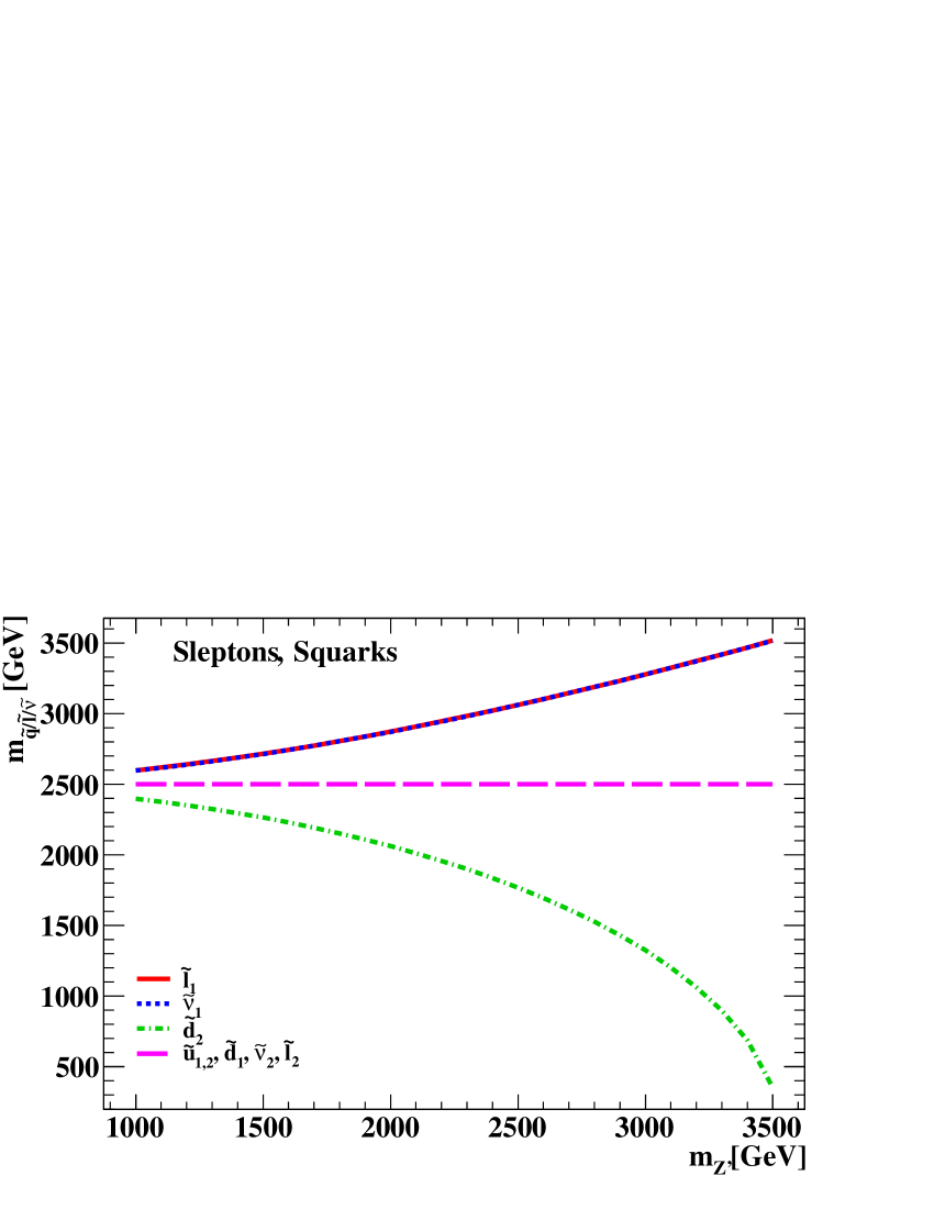
The D-term correction, and therefore the sfermion masses, is also function of the mass: this dependence is studied for the model and the parameters set as in the Representative Point, in the range TeV. In Fig. 2 the squark and slepton masses are plotted with respect to , obtaining quite cumbersome results. The masses of , , and are independent of ; on the contrary, and are degenerate and increase from 2.5 TeV ( TeV) to about 3.5 TeV ( TeV). The mass of is TeV for TeV and for TeV; due to the large negative D-term for squarks, no physical solution for is allowed above TeV.
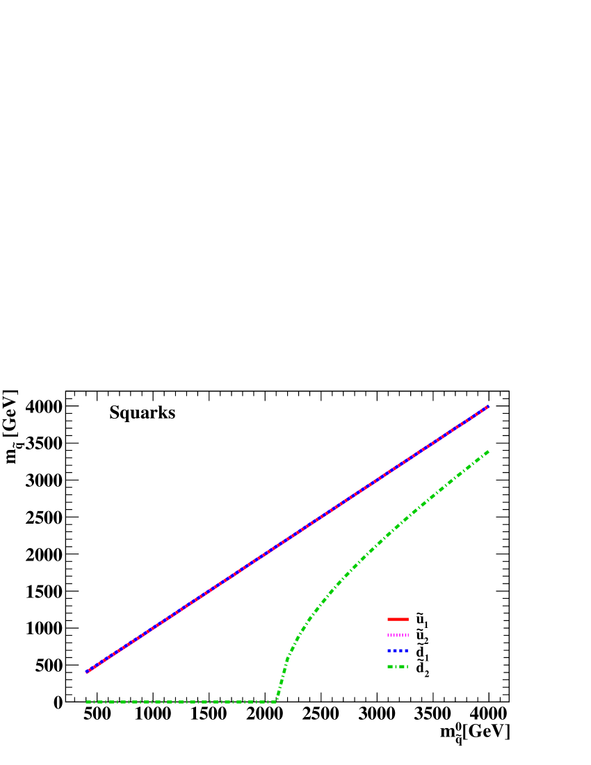
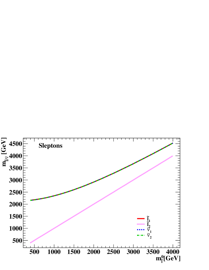
The dependence of the sfermion masses on the initial values and , set at the mass scale, and varied from 400 GeV to 4 TeV, is presented in Fig. 3. As expected, given Eqs. (28)-(30), all sfermion masses are monotonically increasing function of ; in the case of , , and , being the D-term negligible, they are degenerate and approximately equal to in the whole explored range. The mass of the squark is instead physical only for 2.1 TeV and increases up to the value TeV for TeV. The masses , and are also degenerate and vary from about 2.1 TeV ( GeV) to 4.5 TeV ( TeV).
We also studied the variation of the sfermion masses with respect to , in the range , and on the trilinear coupling , for , but found very little dependence on such parameters. Moreover, there is no dependence on , and , which do not enter in the expressions of the sfermion masses, even after the D-term correction.
4.2 Neutralino masses
We wish to study the dependence of the neutralino masses on the parameters playing a role in our analysis: unlike the sfermion masses, they depend also on the gaugino masses , and . Table 3 reports the six neutralino masses for the parametrization in Eq. (31). For TeV, decays into channels containing the heaviest neutralino are not permitted because of phase-space restrictions. and therefore they can be discarded in the Representative Point scenario. Being TeV, decays into states containing are kinematically allowed, but one can already foresee very small branching ratios.
| 94.6 GeV | 156.6 GeV | 212.2 GeV | 261.0 GeV | 2541.0 GeV | 3541.0 GeV |
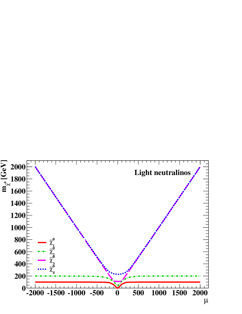
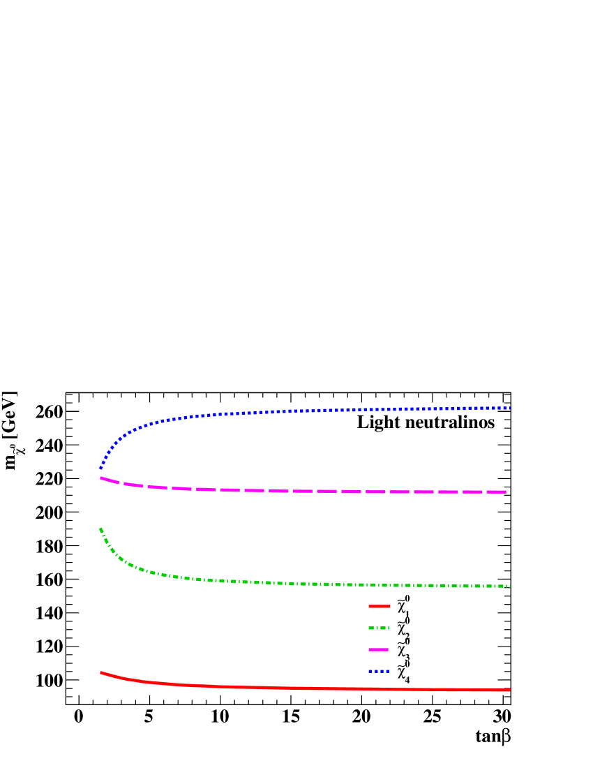
Figure 4 presents the dependence of the mass of the four lightest neutralinos, i.e. , on the supersymmetry parameters (left) and (right), for and , with the others as in Eq. (31). The distribution of the masses of is symmetric with respect to . Nevertheless, and increase from 0 () to about 100 () and 200 GeV () in the range GeV, whereas they are almost constant for . On the contrary, the masses of and exhibit a minimum for , about 110 and 230 GeV respectively, and increase monotonically in terms of , with a behaviour leading to for large . As for , a small dependence is visible only in the low range, i.e. , with the masses of , and slightly decreasing and the one of mildly increasing. Outside this range, the light neutralino masses are roughly independent of .
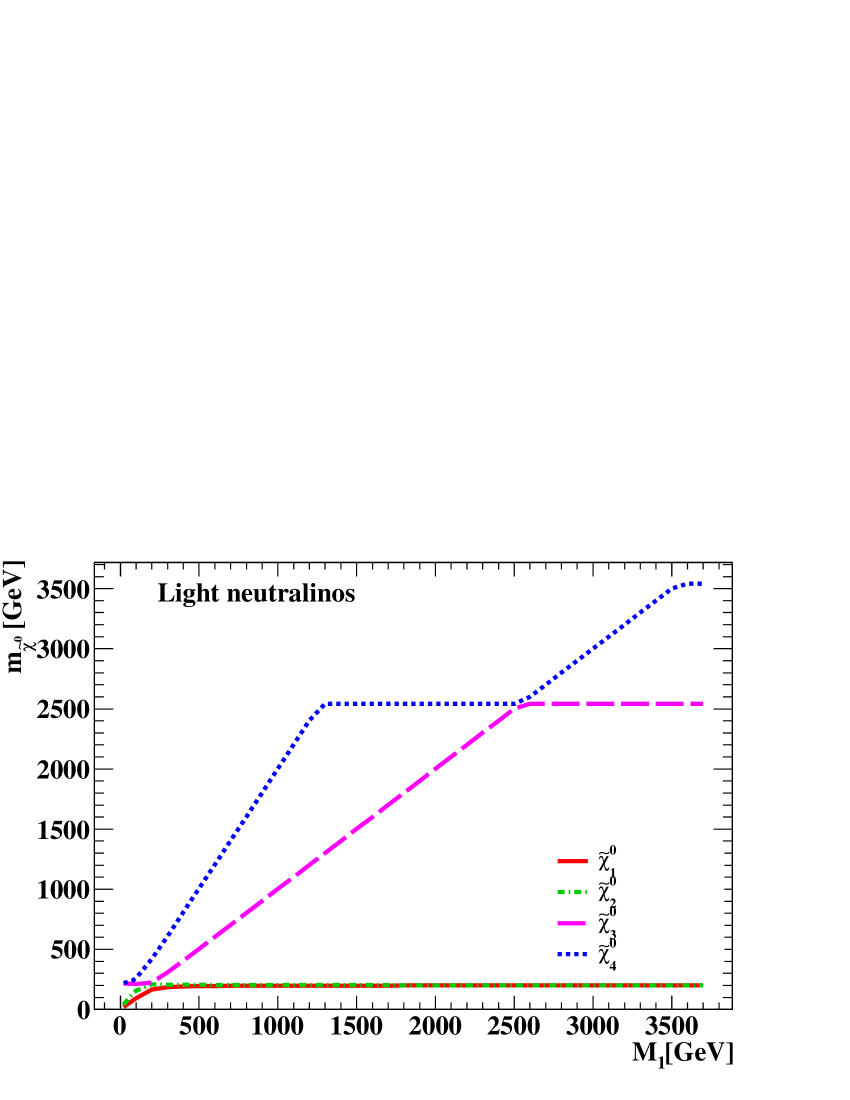
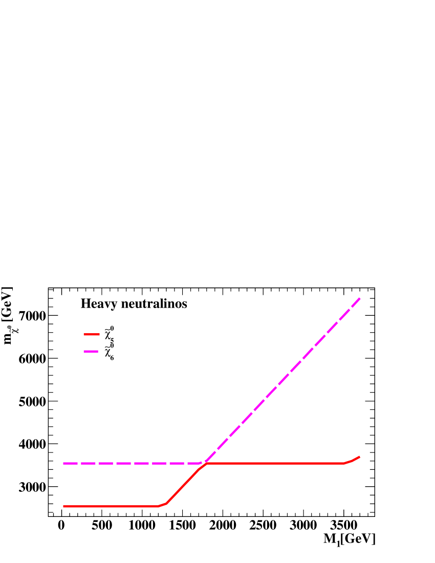
In Fig. 5 we present the dependence of the light (left) and heavy (right) neutralino masses on the gaugino mass for . In the light case, the masses exhibit a step-like behaviour: and have roughly the same value through all range, growing for small and amounting to approximately 200 GeV for GeV. The mass increases in the range and is about TeV for 2.5 TeV. The mass of is roughly for TeV, then TeV, up to TeV, and ultimately for larger . As for the heavy neutralinos, the mass of is TeV for TeV, then it increases linearly in the range TeV and it is TeV for TeV. The mass of the heaviest neutralino is constant, namely TeV, for TeV, then it grows linearly, reaching the value TeV for TeV.
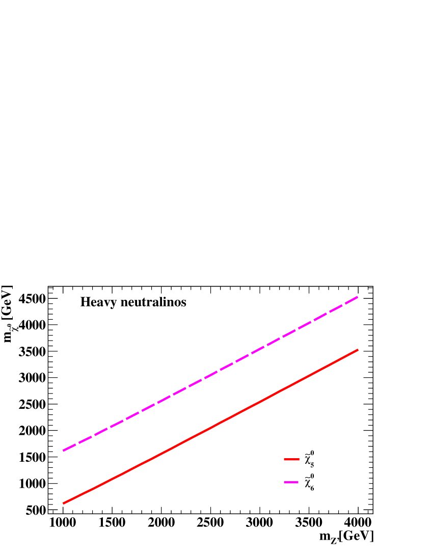
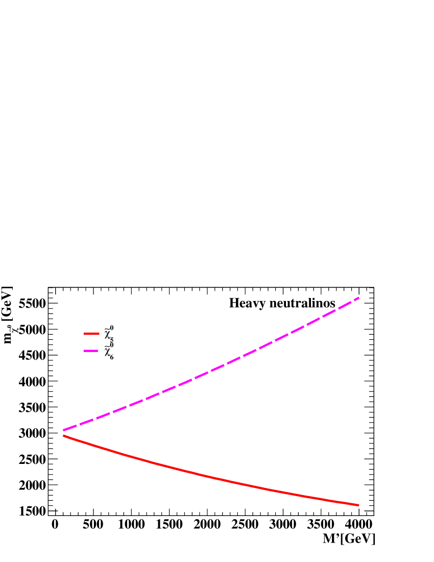
Figure 6 presents the masses of and with respect to the mass in the range 1 TeV 4 TeV (left) and to the parameter for 100 GeV 4 TeV (right). The masses of and grow linearly as a function of , whereas they exhibit opposite behaviour with respect to , as increases from 3 to 5.5 TeV and decreases from 3 to 1.5 TeV. The four light-neutralino masses are instead roughly independent of and , as expected.
4.3 Chargino masses
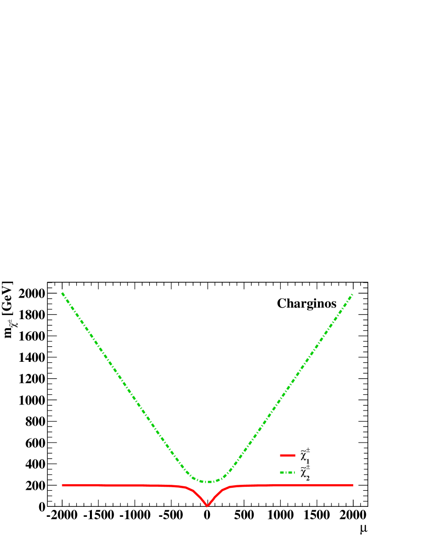
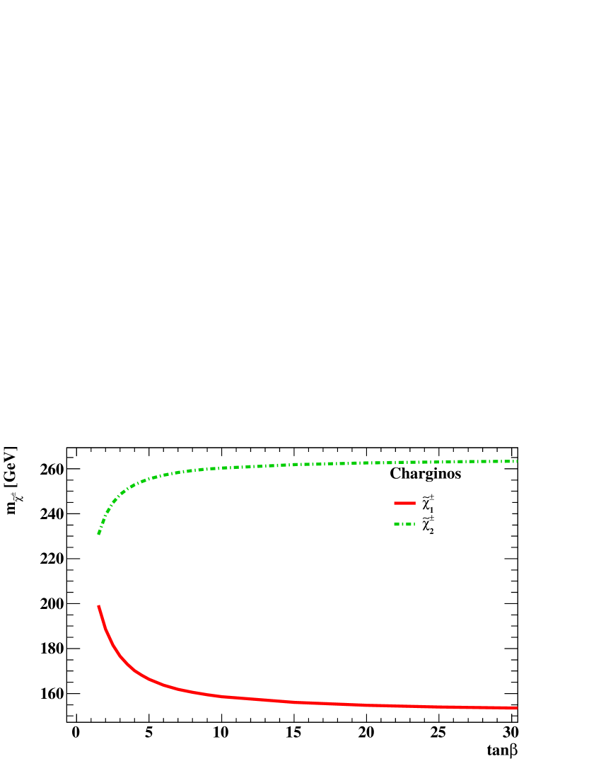
As discussed before, the chargino sector remains unchanged after the introduction of the extra group . Therefore, the chargino masses do not depend on the U(1)′ new parameter and on , but just on the MSSM parameters , and . Figures 7 and 8 show the dependence on such quantities, which are varied individually, with the other parameters fixed as in Eq. (31).
The dependence on , displayed in Fig. 7 (left), is symmetric with respect to . In particular, varies significantly, from about 3 to 200 GeV, only for GeV, whereas the heavier chargino mass exhibits a behaviour and is as large as 2 TeV for GeV. As for , Fig. 7 (right), the mass of the heavy chargino increases quite mildly from 230 to about 263 GeV, whereas decreases from almost 200 GeV () to about 154 GeV ().
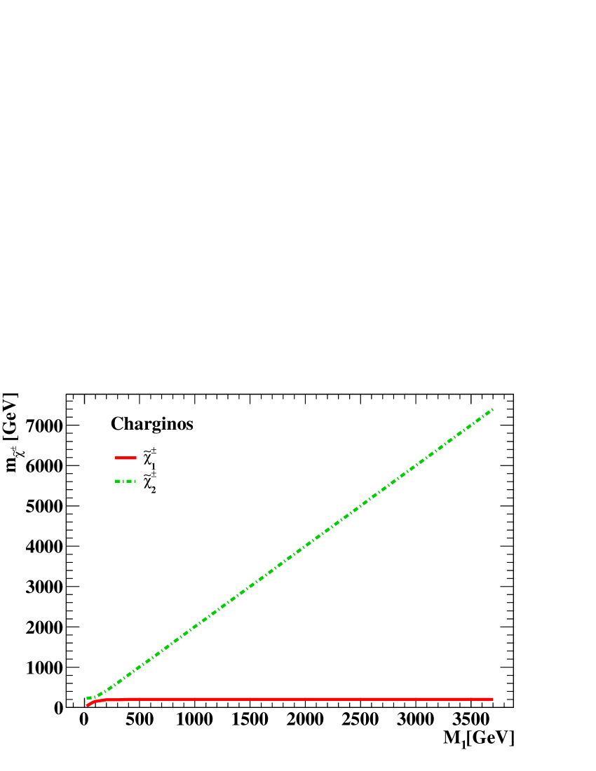
The variation with respect to , presented in Fig. 8, is instead quite different for the two charginos. The mass of the lighter one changes very little only for GeV, whereas for larger it is about GeV. The mass of increases almost linearly with and and is for large .
4.4 Higgs masses
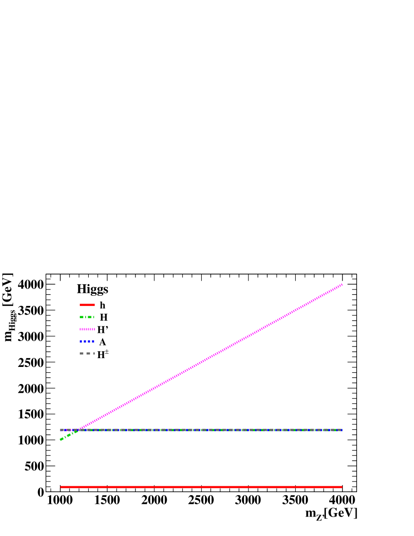
As pointed out before in the paper, after adding the symmetry, one has an extra neutral scalar Higgs, named , besides the Higgs sector of the MSSM, i.e. the bosons , , and . The phenomenology will thus depend on the three Higgs masses and vacuum expectation values , and . In the Representative Point parametrization, the lightest has a mass GeV, , and are degenerate and have a mass of about 1190 GeV, whereas the -inherited is about 3 TeV, like the . Therefore, in this scenario the is not capable of decaying into final states containing .
Figure 9 presents the variation of the Higgs masses in terms of (left) and (right); Fig. 10 shows the dependence on (left) and (right). One can immediately notice that the mass of the lightest is roughly independent of these quantities and it is GeV through the whole , , and ranges. Since the supersymmetric light Higgs should roughly play the role of the SM Higgs boson, a value of about 90 GeV for its mass is too low, given the current limits from LEP [36] and Tevatron [37] experiments and the recent LHC results [38, 39] on the observation of a new Higgs-like particle with a mass about 125 GeV. This is due to the fact that the mass obtained after diagonalizing the neutral Higgs mass matrix is just a tree-level result; the possible inclusion of radiative corrections should increase the light Higgs mass value in such a way to be consistent with the experimental limits. In fact, the Representative Point will be used only to illustrate the features of the particle spectra in the MSSM, after one adds the extra symmetry group. Any realistic analysis of decays in supersymmetry should of course use values of the Higgs masses accounting for higher-order corrections and in agreement with the experimental data.
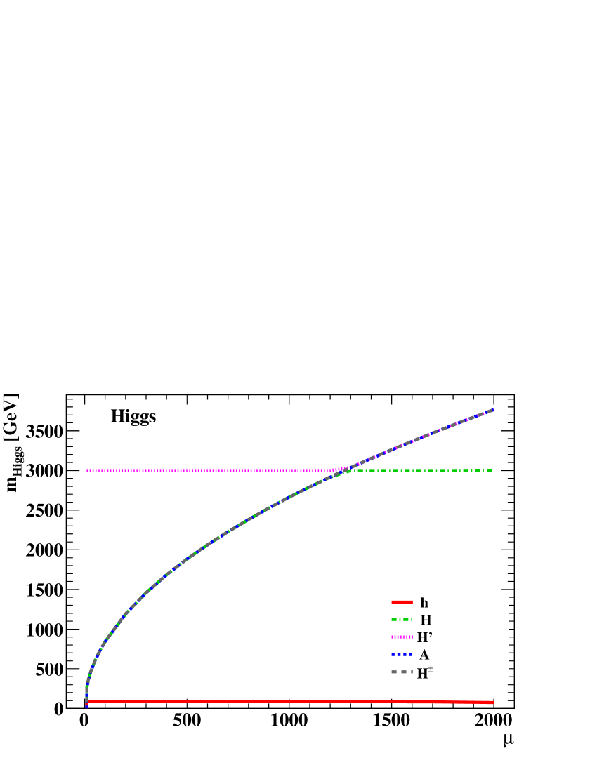
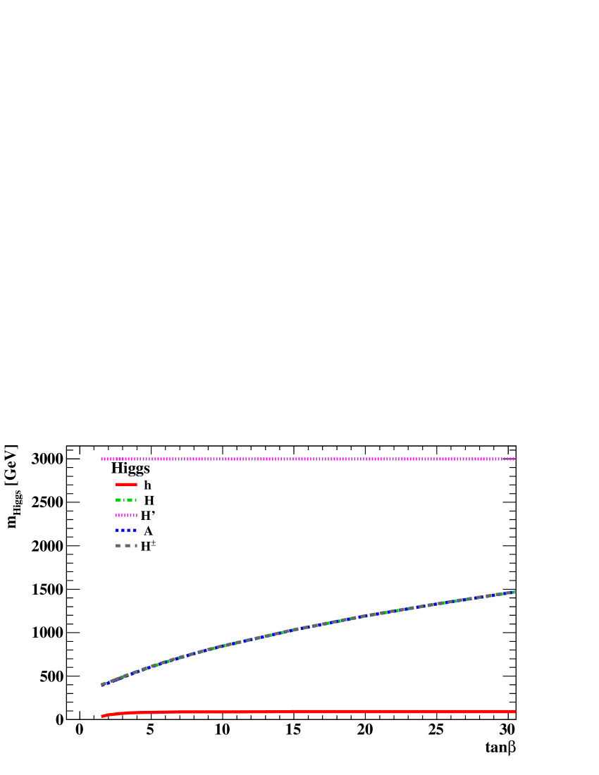
The heavy MSSM scalar Higgs is physical, i.e. its squared mass positive definlite, only for positive values of , therefore in Fig. 9 the Higgs masses are plotted for . The mass of increases monotonically from 0 () to 3 TeV ( GeV), and then it is also for larger -values. As for the -inherited , its mass is about for GeV; for larger it increases monotonically, up to TeV, value reached for GeV. In other words, for GeV, and behave as if they exchanged their roles, with increasing and constant . The masses of and exhibit instead the same behaviour and increase monotonically with respect to in the whole range. It is also interesting to notice that, for GeV, one has . As for the dependence on , presented in Fig. 9 (right), the masses of , and are almost degenerate and increase from about 400 GeV () to approximately 1.5 TeV (). The mass of is instead TeV for any value of .
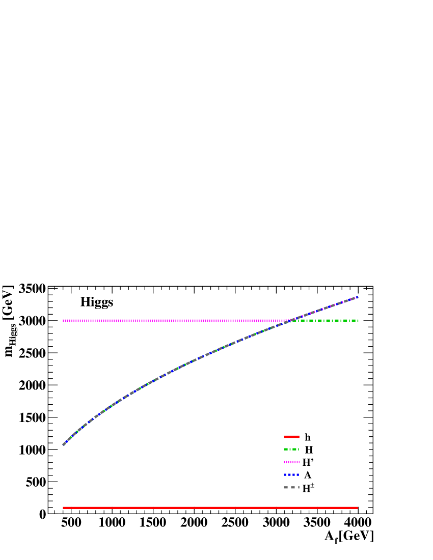
The dependence of the Higgs masses on the mass in the range 1 TeV TeV is presented in Fig. 10 (left). and are degenerate and their mass is constantly equal to 1.19 TeV in the whole explored region. The mass is TeV for TeV, then it slightly increases and amounts to TeV in the range 1.2 TeV TeV. Figure 10 (right) shows the Higgs masses as functions of the trilinear coupling for . The masses of the charged and pseudoscalar Higgs bosons are degenerate and increase from 1.1 TeV ( GeV) to about 3.4 TeV ( TeV). The mass of the scalar neutral is degenerate with the ones of and for , then it is TeV for between 3.2 and 4 TeV. The mass is constant, i.e. TeV for , then it increases in the same manner as the masses of and . As already observed for the dependence, and exchange their roles for TeV.
4.5 Consistency of the MSSM masses with ISAJET
An experimental search for supersymmetric decays demands the implementation of our MSSM/ scenario in a Monte Carlo event generator. Therefore, it is essential to verify whether our mass spectra are consistent with those provided by the codes typically used to compute masses and decay rates in supersymmetry. For this purpose, a widely used program is the ISAJET package [40], containing all the MSSM data; the supersymmetric particle masses and branching ratios obtained by running ISAJET are then used by programs, such as HERWIG [22] and PYTHIA [23], which simulate hard scattering, parton showers, hadronization and underlying event, for an assigned MSSM configuration. It is thus crucial assessing whether such an approach can still be employed even after the inclusion of the extra boson. Squark and slepton masses, corrected by the D-term contribution, can be directly given as an input to ISAJET. Moreover, the chargino spectrum is unchanged, being the neutral, whereas the extra , being too heavy, is not relevant for the phenomenology. Besides, the masses of the MSSM Higgs bosons , , and depend very mildly on the parameters. In the neutralino sector, the two additional and are also too heavy to be phenomenologically relevant. However, the neutralino mass matrix, Eq. (21), depends also on extra new parameters, such as , and the charges . Therefore, even the mass of the four light neutralinos can potentially feel the effect of the presence of the .
We quote in Table 4 the eigenvalues of the neutralino mass matrix, Eq. (21), along with the masses yielded by ISAJET, for the parameter configuration corresponding to the Representative Point, Eq. (31). For the sake of completeness, we also present the Higgs and chargino mass values obtained in our framework ( and MSSM), to investigate whether they agree with the ISAJET results (only MSSM).
| Model | ||||||||||
|---|---|---|---|---|---|---|---|---|---|---|
| /MSSM | 94.6 | 156.6 | 212.2 | 261.0 | 90.7 | 1190.0 | 1190.0 | 1190.0 | 155.0 | 263.0 |
| MSSM | 91.3 | 152.2 | 210.2 | 266.7 | 114.1 | 1190.0 | 1197.9 | 1200.7 | 147.5 | 266.8 |
From Table 4 one learns that the masses of the neutralinos agree within 5%; a larger discrepancy is instead found, about 20%, for the mass of the lightest Higgs, i.e. ; as pointed out before, this difference is due to the fact that, unlike ISAJET, our calculation is just a tree-level one and does not include radiative corrections. Both Higgs masses are nevertheless much smaller than the , fixed to 3 TeV in the Representative Point; therefore, decays into Higgs bosons will not be significantly affected by this discrepancy.
As for the chargino masses, the difference between our analytical calculation and the prediction of ISAJET is approximately 5% for and 1% for . Overall, one can say that some differences in the spectra yielded by our computations and ISAJET are visible, but they should not have much impact on phenomenology. The implementation of the model in HERWIG or PYTHIA, along with the employment of a standalone program like ISAJET for masses and branching ratios in supersymmetry, may thus provide a useful tool to explore phenomenology in an extended MSSM.
4.6 decays in the Representative Point
Before concluding this section, we wish to present the branching ratios of the boson into both SM and new-physics particles. If BSM decays are competitive with the SM ones, then the current limits on the mass will have to be reconsidered. We shall first present the branching ratios in the Representative Point parametrization, Eq. (31), i.e. a boson with mass 3 TeV, and then we will vary the quantities entering in our analysis.
4.6.1 Branching ratios in the Representative Point
In Table 5 we summarize, for the reader’s convenience, the masses of the BSM particles for the parameters in Eq. (31), in such a way to figure out the decay channels which are kinematically permitted.
| 2499.4 | 2499.7 | 2500.7 | 1323.1 | 3279.0 | 2500.4 | 3278.1 | 3279.1 |
| 94.6 | 156.5 | 212.2 | 260.9 | 2541.4 | 3541.4 | 154.8 | 262.1 |
| 90.7 | 1190.7 | 1190.7 | 3000.0 | 1193.4 |
At this point it is possible to calculate the widths into the kinematically allowed decay channels. The SM decay channels are the same as the boson, i.e. quark or lepton pairs, with the addition of the mode, which is accessible due to the higher mass. However, since the has no direct coupling to bosons, the occurs only via mixing and therefore one can already foresee small branching ratios. Furthermore, the extended MSSM allows decays into squarks, i.e. ( and ), charged sleptons , sneutrinos (, , , ), neutralino, chargino, or Higgs (, , , , , , ) pairs, as well as into states with Higgs bosons associated with , such as , and .
We refer to [12] for the analytical form of such widths, at leading order in the coupling constant, i.e. ; in Appendix A the main formulas will be summarized. Summing up all partial rates, one can thus obtain the total width and the branching ratios into the allowed decay channels.
In Table 6 we quote the branching ratios in the Representative Point parametrization. Since, at the scale of 3 TeV, one does not distinguish the quark or lepton flavour, the quoted branching ratios are summed over all possible flavours and , , and denote any possible up-, down-type quark, charged-lepton or neutrino pair. Likewise, , , and are their supersymmetric counterparts. We present separately the branching ratios into all possible different species of charginos and neutralinos, as they yield different decay chains and final-state configurations.
| Final state | BR | Final state | BR |
|---|---|---|---|
| 0.00 | 0.07 | ||
| 40.67 | 0.43 | ||
| 13.56 | 0.71 | ||
| 27.11 | 0.27 | ||
| 0.00 | |||
| 9.58 | 0.65 | ||
| 0.00 | 2.13 | ||
| 0.00 | 0.80 | ||
| 0.50 | 1.75 | ||
| 1.31 | |||
| 0.51 | |||
| 0.25 | |||
| 0.00 | 0.00 | ||
| 0.00 | 0.00 | ||
| 1.76 | |||
| 1.95 | |||
| 0.54 |
In Table 6, several branching ratios are zero or very small: the decays into up-type squarks and sleptons, heavy neutralinos and the -inherited are kinematically forbidden for a of 3 TeV. The only allowed decay into sfermion pairs is the one into down-type squarks . Despite being kinematically permitted, the width into up-type quarks vanishes, since, as will be clarified in Appendix A, in the model the vector () and vector-axial () couplings, contained in the in the interaction Lagrangian of the with up quarks, are zero. From Table 6 we learn that, at the Representative Point, the SM decays account for roughly the 77% of the total width and the BSM ones for the remaining 23%. As for the BSM modes, the rate into down squarks is about 9% of the total rate, the ones into charginos and neutralinos 4.2% and 8.4%, respectively. In the gaugino sector, the channels and have the highest branching ratios. The decay into has a very small branching fraction and is experimentally undetectable if is the lightest supersymmetric particle (LSP). The final states with Higgs bosons are characterized by very small rates: the branching fractions into and are about 0.5%, the one into roughly 0.1% and an even lower rate, , is yielded by the modes , and .
These considerations, obtained in the particular configuration of the Reference Point, Eq. (31), can be extended to a more general context. We can then conclude that the BSM branching fractions are not negligible and should be taken into account in the evaluation of the mass limits.
4.6.2 Parameter dependence of the branching ratios
In this subsection we wish to investigate how the branching fractions into SM and supersymmetric particles fare with respect to the and MSSM parameters. As in Section 3, the study will be carried out at the Representative Point, varying each parameter individually.
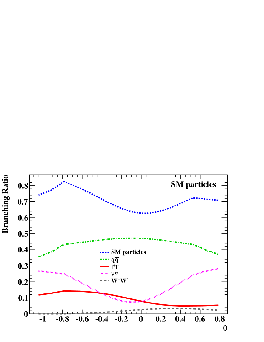
In Fig. 11, the dependence of the branching ratios on the mixing angle is presented for SM (left) and BSM (right) decay modes, in the range ; for the SM channels, we have also plotted the total branching ratio. The decay rate into quarks exhibits a quite flat distribution, amounting to about 40% for central values of and slightly decreasing for large . The branching ratio into neutrino pairs is enhanced for at the edges of the explored range, being about 25%, and presents a minimum for . The rate into charged leptons varies between 5 and 15%, with a small enhancement around ; the branching fraction into is below 2% in the whole range.
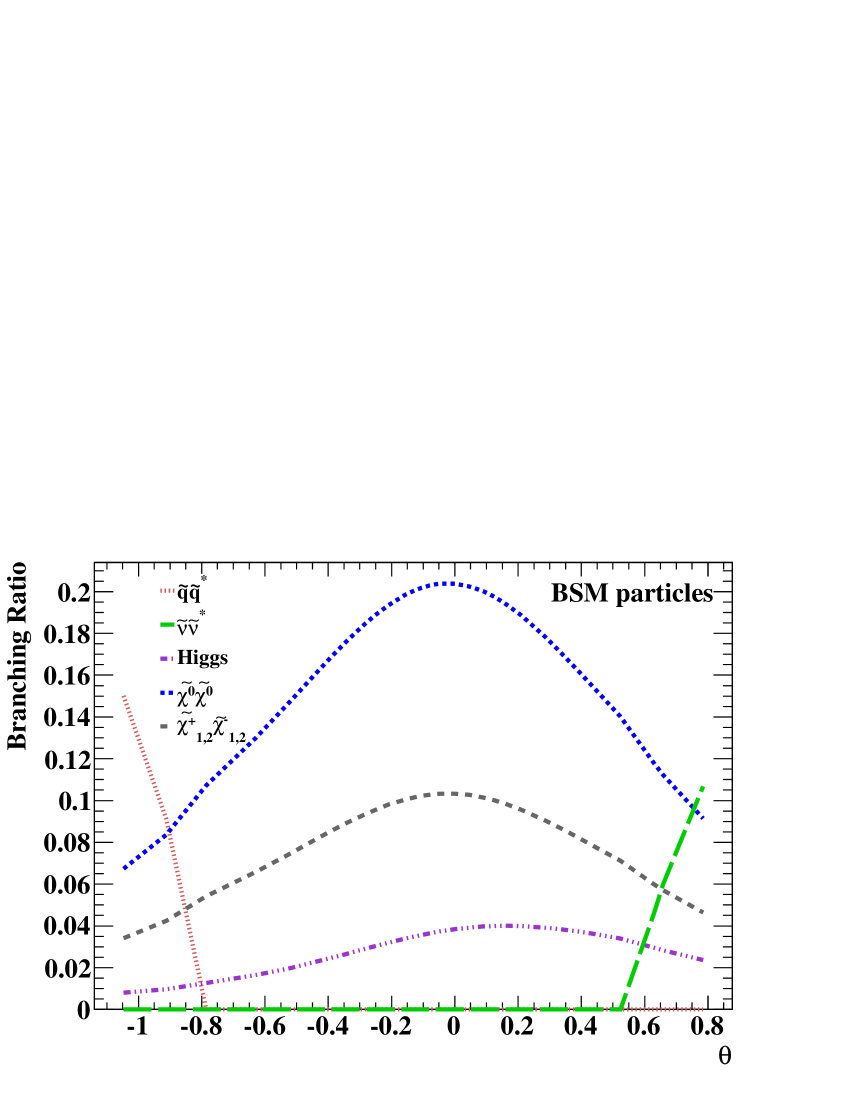
As for the BSM channels, described in Fig. 11 (right), the neutralino, chargino, and Higgs modes have a similar behaviour, with a central broad maximum around and branching ratios about 20%, 10% and 3%, respectively The sneutrino modes give a non-negligible contribution only for , reaching about 10%, at the boundary of the investigated region, i.e. . The squark-pair channel has a significant rate, about 15%, for negative mixing angles, i.e. . The rates in the Higgs channels lie between the neutralino and chargino ones and exhibit a maximum value, about 10%, for .
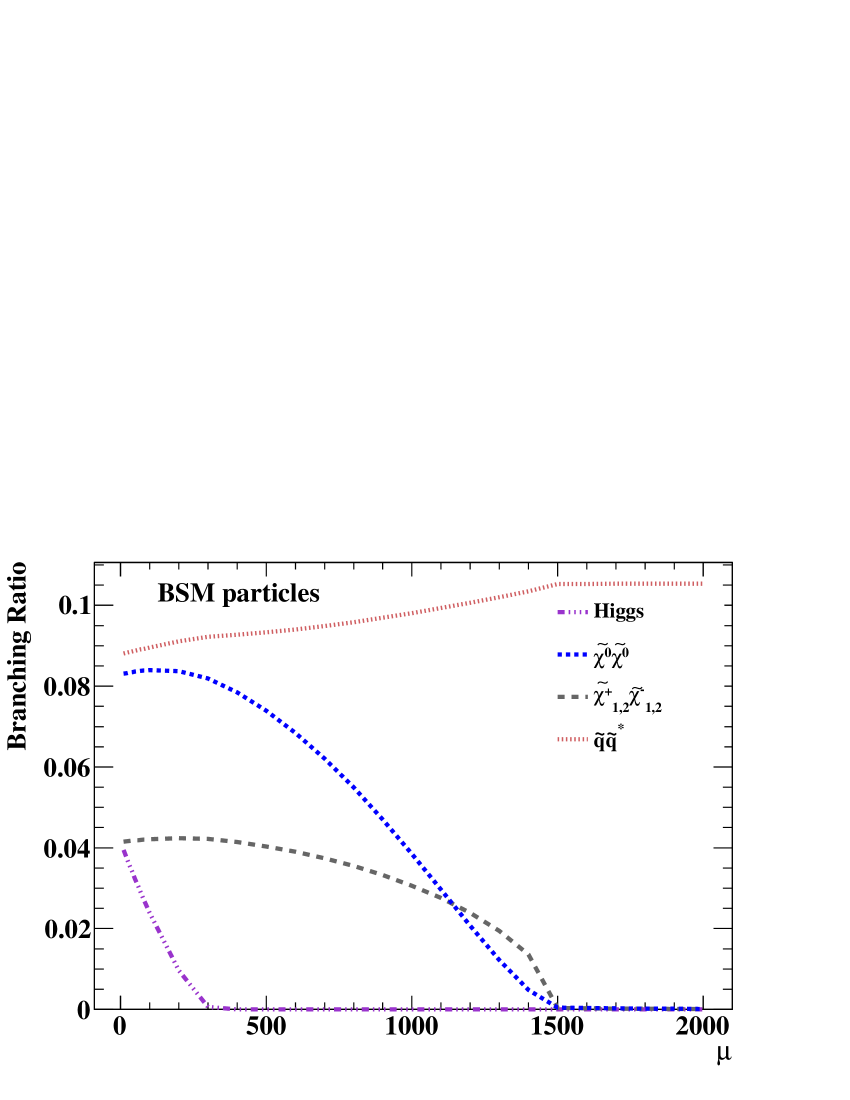
Figure 12 presents the dependence of the BSM branching ratios on the MSSM parameters (left) and (right). The SM rates are not shown, since their dependence on these parameters is negligible. The decay rate into squarks slightly increases from 9 to 10% in the explored range; the neutralino branching ratio decreases quite rapidly from about 8% () to zero ( GeV). The rate into charginos is about 4% for small values of , then it smoothly decreases, being negligible for GeV. The branching fraction into Higgs modes is almost 4% at and rapidly becomes nearly zero for GeV. As for , the , and modes are roughly independent of it, with rates about 9% (squarks), 8% (neutralinos) and 4% (charginos). The decays into states with Higgs bosons account for 4% of the width at small and are below for .
5 decays into final states with leptons
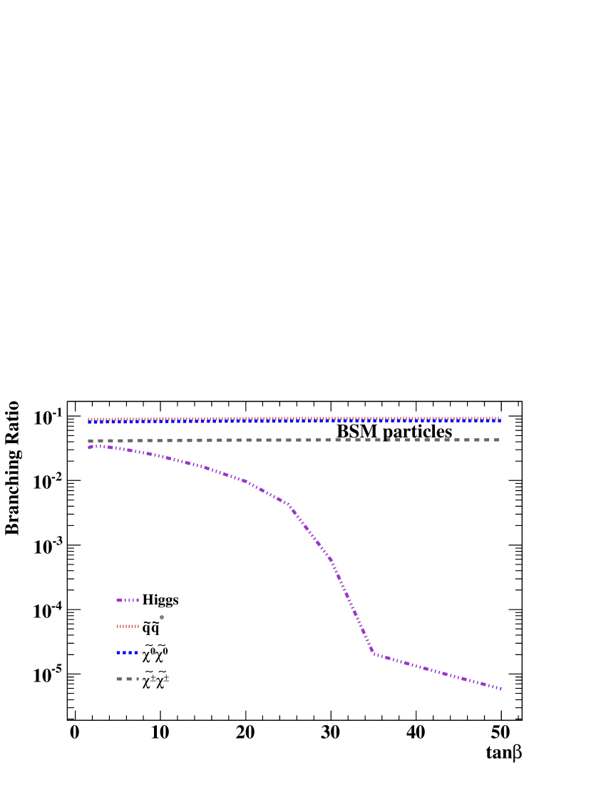
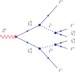
Leptonic final states are considered as golden channels from the viewpoint of the LHC experimental searches. To exploit these features, this study will be focused on the decays of the boson into supersymmetric particles, leading to final states with leptons and missing energy, due to the presence of neutralinos or neutrinos. Final states with two charged leptons and missing energy come from primary decays , presented in Fig. 13, with the charged sleptons decaying into a lepton and a neutralino.
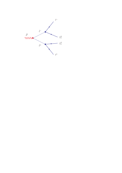
Furthermore, primary decays into charginos , followed by and (), as in Fig. 14, yield final states with two charged leptons and missing energy as well. With respect to the direct production in collisions, where the partonic centre-of-mass energy is not uniquely determined, the production of charginos in decays has the advantage that the mass sets a kinematic constrain on the chargino invariant mass.
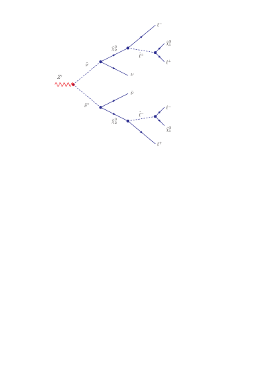
A decay chain, leading to four charged leptons and missing energy, is yielded by decays into neutralinos , with subsequent and , as in Fig. 15. Finally, we shall also investigate the decay into sneutrino pairs, such as , followed by and , with an intermediate charged slepton (see Fig. 16). The final state of the latest decay chain is made of four charged leptons plus missing energy, due to neutrinos and neutralinos.
In the following, we wish to present a study of decays into leptonic final states for a given set of the MSSM and parameters. In particular, we shall be interested in understanding the behaviour of such rates as a function of the slepton mass, which will be treated as a free parameter. In order to increase the rate into sleptons, with respect to the scenario yielded by the Representative Point, the squark mass at the scale will be increased to 5 TeV, in such a way to suppress decays into hadronic jets.
In our study we consider the models in Table 1 and vary the initial slepton mass for several fixed values of , with the goal of determining an optimal combination of and , enhancing the rates into leptonic final states, i.e. the decay modes containing primary sleptons, charginos or neutralinos. The other parameters are set to the following Reference Point:
| (33) | |||||
Any given parametrization will be taken into account only if the sfermion masses are physical after the addition of the D-term. Hereafter, we denote by , , and the branching ratios into quark, charged-lepton, neutrino and pairs, with BRSM being the total SM decay rate. Likewise, BR, BR and BR are the rates into squarks, charged sleptons and sneutrinos, , , , , are the ones into chargino, neutralino, charged- and neutral-Higgs pairs, the branching fraction into . Moreover, for convenience, is the sum of the branching ratios into and and BRBSM the total BSM branching ratio.
5.1 Reference Point: Model
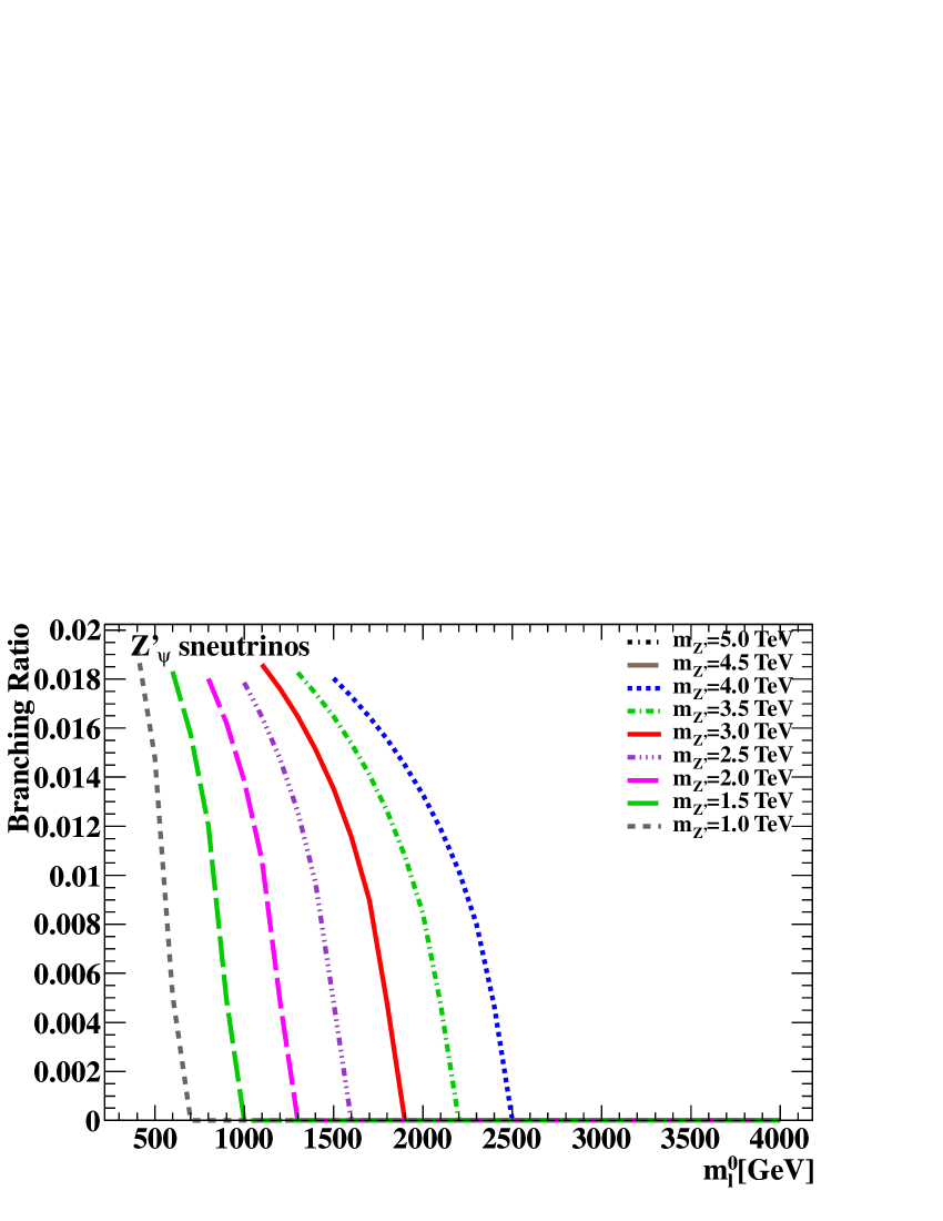
An extra group with a mixing angle leads to a new neutral boson labelled as . In Table 7 we list the masses of charged ( and ) and neutral ( and ) sleptons, for various and for the values of which, as will be clarified later, yield a physical sfermion spectrum and a maximum and minimum rate into sneutrinos. From Table 7 we learn that the decays into pairs of charged sleptons are always kinematically forbidden, whereas the decay into pairs is accessible. The effect of the D-term on the mass of is remarkable: variations of of few hundreds GeV induce in a change of 1 TeV or more, especially for large values of the mass.
| 1000 | 800 | 736.9 | 665.9 | 732.6 | 379.3 |
|---|---|---|---|---|---|
| 1000 | 900 | 844.4 | 783.2 | 840.6 | 560.2 |
| 1500 | 1100 | 994.0 | 873.8 | 990.8 | 298.0 |
| 1500 | 1300 | 1211.6 | 1115.1 | 1209.0 | 754.2 |
| 2000 | 1500 | 1361.2 | 1205.6 | 1358.9 | 503.8 |
| 2000 | 1800 | 1686.1 | 1563.1 | 1684.2 | 1115.3 |
| 2500 | 1800 | 1618.0 | 1411.9 | 1616.1 | 344.7 |
| 2500 | 2200 | 2053.8 | 1895.6 | 2052.2 | 1311.0 |
| 3000 | 2200 | 1985.7 | 1744.6 | 1984.1 | 586.4 |
| 3000 | 2600 | 2421.4 | 2227.9 | 2420.0 | 1504.6 |
| 3500 | 2500 | 2242.3 | 1950.2 | 2240.9 | 358.9 |
| 3500 | 3100 | 2896.2 | 2676.5 | 2895.1 | 1867.8 |
| 4000 | 2900 | 2610.2 | 2283.3 | 2608.9 | 643.3 |
| 4000 | 3500 | 3263.9 | 3008.9 | 3262.9 | 2062.5 |
| BR | BR | ||||||||||
|---|---|---|---|---|---|---|---|---|---|---|---|
| 1.0 | 0.8 | 39.45 | 5.24 | 27.26 | 3.01 | 2.91 | 4.92 | 8.64 | 8.54 | 74.97 | 25.03 |
| 1.0 | 0.9 | 43.14 | 5.73 | 29.81 | 3.30 | 3.18 | 5.38 | 9.45 | 0.00 | 81.98 | 18.02 |
| 1.5 | 1.1 | 37.82 | 4.93 | 25.63 | 2.71 | 2.67 | 5.16 | 9.76 | 11.31 | 71.10 | 28.90 |
| 1.5 | 1.3 | 42.65 | 5.56 | 28.90 | 3.06 | 3.01 | 5.82 | 11.00 | 0.00 | 80.16 | 19.84 |
| 2.0 | 1.5 | 37.97 | 4.91 | 25.54 | 2.66 | 2.64 | 5.33 | 10.33 | 10.61 | 71.48 | 28.52 |
| 2.0 | 1.8 | 42.47 | 5.49 | 28.57 | 2.98 | 2.95 | 5.96 | 11.56 | 0.00 | 79.52 | 20.48 |
| 2.5 | 1.8 | 37.46 | 4.83 | 25.12 | 2.60 | 2.59 | 5.33 | 10.44 | 11.61 | 70.02 | 29.98 |
| 2.5 | 2.2 | 42.39 | 5.47 | 28.42 | 2.94 | 2.93 | 6.02 | 11.81 | 0.00 | 79.21 | 20.79 |
| 3.0 | 2.2 | 37.60 | 4.84 | 25.17 | 2.59 | 2.59 | 5.38 | 10.61 | 11.14 | 70.19 | 29.81 |
| 3.0 | 2.6 | 42.31 | 5.45 | 28.32 | 2.92 | 2.91 | 6.06 | 11.94 | 0.00 | 78.64 | 21.36 |
| 3.5 | 2.5 | 37.30 | 4.80 | 24.94 | 2.56 | 2.56 | 5.36 | 10.61 | 11.73 | 69.59 | 30.41 |
| 3.5 | 3.1 | 42.26 | 5.43 | 28.25 | 2.90 | 2.90 | 6.07 | 12.02 | 0.00 | 78.84 | 21.16 |
| 4.0 | 2.9 | 37.41 | 4.81 | 25.00 | 2.56 | 2.56 | 5.39 | 10.70 | 11.38 | 69.78 | 30.22 |
| 4.0 | 3.5 | 42.22 | 5.43 | 28.21 | 2.89 | 2.89 | 6.08 | 12.07 | 0.00 | 78.74 | 21.26 |
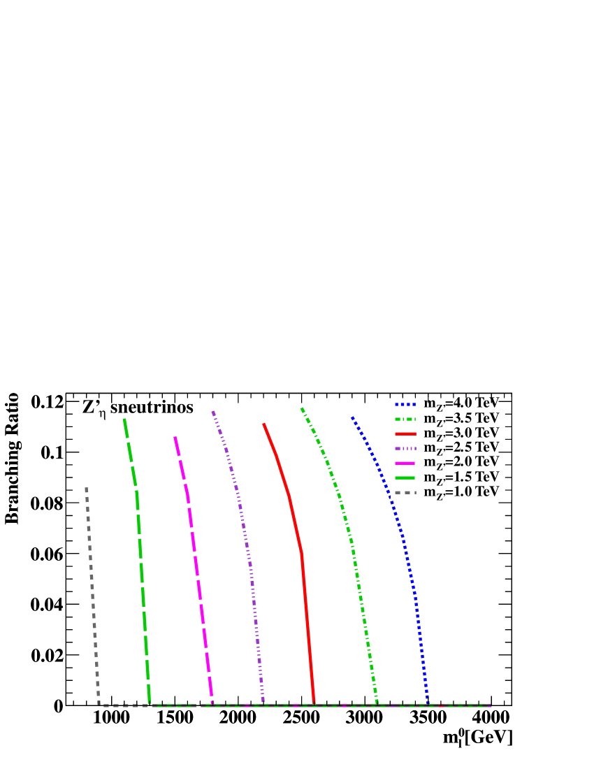
Table 8 summarizes the branching ratios into all allowed SM and BSM channels, for the same and values as in Table 7, whereas Fig. 17 presents the branching ratio as a function of and for 1 TeV 4 TeV. The branching fraction into sneutrinos can be as large as about 11% for any value of ; for larger the sneutrino rate decreases, as displayed in Fig. 17. Furthermore, Table 8 shows that, within the scenario identified by the Reference Point, even the decays into charginos and neutralinos are accessible, with branching ratios about 5-6% (charginos) and 10-12% (neutralinos). Decays into pairs or Higgs bosons associated with ’s are also permitted, with rates about 3%. The decrease of the sneutrino rate for large results in an enhancement of the SM branching ratios into and neutrino pairs. As a whole, summing up the contributions from sneutrinos, charginos and neutralinos, the branching ratio into BSM particles runs from 24 to 33%, thus displaying the relevance of those decays in any analysis on production in a supersymmetric scenario.
5.2 Reference Point:
An extra group with a mixing angle leads to a neutral vector boson labelled as (Table 1). In Table 9, we quote the slepton masses for a few values of and : as before, the results are presented for the two values of which are found to enhance and minimize the slepton rate. For any mass value, the D-term enhances by few hundreds GeV the masses of and and strongly decreases and , especially for small and large . In Table 10 we present the branching ratios into all channels, for the same values of and as in Table 9. Unlike the case, supersymmetric decays into charged-slepton pairs are allowed for , with a branching ratio, about 2%, roughly equal to the sneutrino rate. Furthermore, even the decays into gauginos are relevant, with rates into and about 10 and 20%, respectively. The decays into boson pairs, i.e. and , are also non-negligible and account for about 3% of the total width.
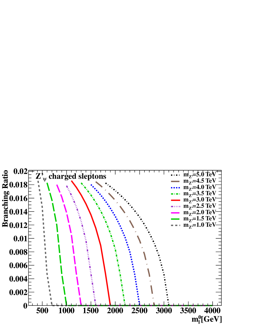
As a whole, the modelling above depicted yields branching ratios of the order of 35-40% into BSM particle, and therefore it looks like being a promising scenario to investigate production within the MSSM. Figure 18 finally displays the branching ratios into sneutrinos and charged sleptons as a function of and for several values of .
| 1000 | 400 | 535.2 | 194.2 | 529.2 | 189.2 |
|---|---|---|---|---|---|
| 1000 | 700 | 785.1 | 606.4 | 781.0 | 604.8 |
| 1500 | 600 | 801.7 | 285.4 | 797.7 | 282.0 |
| 1500 | 1000 | 1132.6 | 849.4 | 112.7 | 848.3 |
| 2000 | 800 | 1068.4 | 377.8 | 1065.4 | 375.2 |
| 2000 | 1300 | 1480.3 | 1092.1 | 1478.2 | 1091.2 |
| 2500 | 1000 | 1335.2 | 470.6 | 1333.8 | 468.6 |
| 2500 | 1600 | 1828.3 | 1334.7 | 1826.6 | 1334.0 |
| 3000 | 1100 | 1528.5 | 296.2 | 1526.4 | 292.9 |
| 3000 | 1900 | 2176.3 | 1577.2 | 2174.9 | 1576.6 |
| 3500 | 1300 | 1795.2 | 401.8 | 1793.4 | 399.4 |
| 3500 | 2200 | 2524.4 | 1819.7 | 2523.2 | 1819.2 |
| 4000 | 1500 | 2061.9 | 502.7 | 2060.4 | 500.8 |
| 4000 | 2500 | 2872.5 | 2062.2 | 2871.4 | 2061.7 |
| 4500 | 1600 | 2256.7 | 177.4 | 2255.3 | 171.9 |
| 4500 | 2800 | 3220.7 | 2304.7 | 3219.7 | 2304.2 |
| 5000 | 1800 | 2523.2 | 343.1 | 2521.9 | 340.3 |
| 5000 | 3100 | 3568.8 | 2547.1 | 3567.9 | 2546.7 |
| BR | BR | |||||||||||
|---|---|---|---|---|---|---|---|---|---|---|---|---|
| 1.0 | 0.4 | 48.16 | 8.26 | 8.26 | 3.00 | 2.89 | 9.13 | 16.53 | 1.91 | 1.90 | 67.69 | 32.31 |
| 1.0 | 0.7 | 50.07 | 8.59 | 8.59 | 3.08 | 2.99 | 9.49 | 17.18 | 0.00 | 0.00 | 70.33 | 29.67 |
| 1.5 | 0.6 | 46.78 | 7.90 | 7.90 | 2.71 | 2.69 | 9.73 | 18.64 | 1.83 | 1.83 | 65.28 | 34.72 |
| 1.5 | 1.0 | 48.55 | 8.20 | 8.20 | 2.81 | 2.79 | 10.10 | 19.35 | 0.00 | 0.00 | 67.76 | 32.24 |
| 2.0 | 0.8 | 46.30 | 7.77 | 7.77 | 2.62 | 2.62 | 9.92 | 19.37 | 1.80 | 1.80 | 64.47 | 35.53 |
| 2.0 | 1.3 | 48.03 | 8.06 | 8.06 | 2.72 | 2.72 | 10.29 | 20.10 | 0.00 | 0.00 | 66.88 | 33.12 |
| 2.5 | 1.0 | 46.01 | 7.70 | 7.70 | 2.58 | 2.59 | 9.99 | 19.68 | 1.79 | 1.78 | 64.00 | 36.00 |
| 2.5 | 1.6 | 47.72 | 7.99 | 7.99 | 2.67 | 2.68 | 10.36 | 20.41 | 0.00 | 0.00 | 66.37 | 33.63 |
| 3.0 | 1.1 | 45.35 | 7.58 | 7.58 | 2.53 | 2.54 | 9.92 | 19.63 | 1.86 | 1.86 | 63.04 | 36.96 |
| 3.0 | 1.9 | 47.10 | 7.88 | 7.88 | 2.62 | 2.64 | 10.30 | 20.39 | 0.00 | 0.00 | 65.47 | 34.53 |
| 3.5 | 1.3 | 44.91 | 7.50 | 7.50 | 2.49 | 2.51 | 9.86 | 19.58 | 1.83 | 1.83 | 62.41 | 37.59 |
| 3.5 | 2.2 | 46.61 | 7.79 | 7.79 | 2.59 | 2.61 | 10.24 | 20.32 | 0.00 | 0.00 | 64.78 | 35.22 |
| 4.0 | 1.5 | 44.60 | 7.45 | 7.45 | 2.47 | 2.49 | 9.82 | 19.53 | 1.80 | 1.80 | 61.96 | 38.04 |
| 4.0 | 2.5 | 46.26 | 7.72 | 7.72 | 2.56 | 2.58 | 10.19 | 20.26 | 0.00 | 0.00 | 64.27 | 35.73 |
| 4.5 | 1.6 | 44.32 | 7.40 | 7.40 | 2.45 | 2.47 | 9.78 | 19.47 | 1.84 | 1.84 | 61.56 | 38.44 |
| 4.5 | 2.8 | 46.01 | 7.68 | 7.68 | 2.54 | 2.57 | 10.15 | 20.21 | 0.00 | 0.00 | 63.91 | 36.09 |
| 5.0 | 1.8 | 44.16 | 7.37 | 7.37 | 2.44 | 2.46 | 9.76 | 19.44 | 1.82 | 1.82 | 61.33 | 38.67 |
| 5.0 | 3.1 | 45.83 | 7.65 | 7.65 | 2.53 | 2.55 | 10.13 | 20.18 | 0.00 | 0.00 | 63.65 | 36.35 |
5.3 Reference Point:
In this subsection we investigate the phenomenology of the boson, i.e. a gauge group with a mixing angle (Table 1), along the lines of the previous sections. As discussed above, the model is interesting since it corresponds to the model, but with the unconventional assignment of the SO(10) representations. Referring to the notation in Eq. (5), in the unconventional E6 model the fields and are in the representation 16 and and in the 10 of SO(10).
Table 11 presents the slepton masses varying and for the values of which minimize and maximize the slepton rate. The D-term addition to increases the mass of and and decreases the mass of ; its impact on is negligible and one can assume . Both decays into and are kinematically allowed, whereas and are too heavy to contribute to the width.
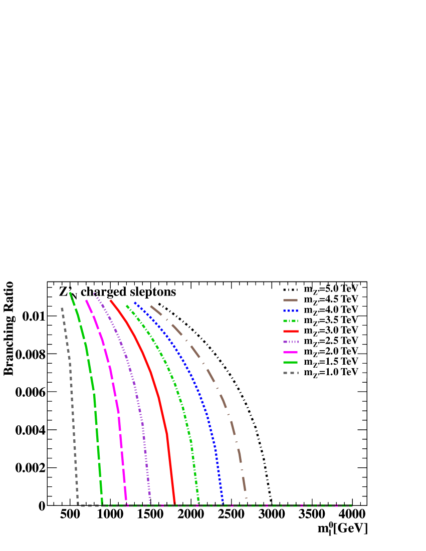
Table 12 quotes the branching ratios for the , computed for the same values of and as in Table 11. Although is kinematically allowed, the coupling of the to sneutrinos is zero for , since, as will be discussed in Appendix A, the rate into right-handed sfermions vanishes for equal vector and vector-axial coupling, i.e. : therefore, this decay mode can be discarded. As for the other supersymmetric channels, the rates into charginos and neutralinos are quite significant and amount to about 9% and 28%, respectively. The decays into and states account for approximately 1-2%, whereas the branching ratio into charged-slepton pairs is about 1%, even in the most favourable case. As a whole, the rates into BSM final states run from 18 to about 35% and therefore are a relevant contribution to the total cross section. Figure 19 finally presents the variation of the charged-slepton branching ratio as a function of , for a few values of .
| 1000 | 400 | 601.1 | 249.7 | 595.8 | 400.0 |
|---|---|---|---|---|---|
| 1000 | 600 | 749.2 | 512.2 | 745.0 | 600.0 |
| 1500 | 500 | 837.4 | 165.4 | 833.6 | 500.0 |
| 1500 | 900 | 1123.1 | 766.4 | 1120.2 | 900.0 |
| 2000 | 700 | 1136.4 | 303.9 | 1133.6 | 700.0 |
| 2000 | 1200 | 1497.1 | 1021.0 | 1495.0 | 1200.0 |
| 2500 | 800 | 1375.8 | 131.8 | 1372.9 | 800.0 |
| 2500 | 1500 | 1871.2 | 1275.7 | 1869.5 | 1500.0 |
| 3000 | 1000 | 1673.7 | 319.9 | 1671.8 | 1000.0 |
| 3000 | 1800 | 2245.3 | 1530.4 | 2243.9 | 1800.0 |
| 3500 | 1200 | 1972.6 | 466.2 | 1971.0 | 1200.0 |
| 3500 | 2100 | 2619.4 | 1785.3 | 2618.2 | 2100.0 |
| 4000 | 1300 | 2211.6 | 303.9 | 2210.2 | 1300.0 |
| 4000 | 2400 | 2993.6 | 2040.2 | 2992.5 | 2400.0 |
| 4500 | 1500 | 2510.2 | 476.8 | 2509.0 | 1500.0 |
| 4500 | 2700 | 3367.7 | 2295.1 | 3366.7 | 2700.0 |
| 5000 | 1600 | 2749.8 | 249.7 | 2748.6 | 1600.0 |
| 5000 | 3100 | 3822.5 | 2666.9 | 3821.6 | 3100.0 |
| BR | |||||||||||
|---|---|---|---|---|---|---|---|---|---|---|---|
| 1.0 | 0.4 | 49.51 | 11.98 | 9.59 | 1.71 | 1.68 | 8.71 | 15.78 | 1.04 | 72.79 | 27.21 |
| 1.0 | 0.6 | 50.03 | 12.11 | 9.69 | 1.73 | 1.69 | 8.80 | 15.94 | 0.00 | 73.56 | 26.44 |
| 1.5 | 0.5 | 47.99 | 11.51 | 9.21 | 1.57 | 1.57 | 9.26 | 17.76 | 1.12 | 70.28 | 29.72 |
| 1.5 | 0.9 | 48.53 | 11.64 | 9.31 | 1.59 | 1.59 | 9.36 | 17.96 | 0.00 | 71.08 | 28.92 |
| 2.0 | 0.7 | 47.50 | 11.36 | 9.08 | 1.53 | 1.54 | 9.44 | 18.46 | 1.08 | 69.47 | 30.53 |
| 2.0 | 1.2 | 48.02 | 11.48 | 9.18 | 1.54 | 1.55 | 9.55 | 18.66 | 0.00 | 70.22 | 29.78 |
| 2.5 | 0.8 | 47.16 | 11.26 | 9.01 | 1.50 | 1.52 | 9.50 | 18.73 | 1.12 | 68.92 | 31.08 |
| 2.5 | 1.5 | 47.69 | 11.38 | 9.11 | 1.52 | 1.53 | 9.61 | 18.94 | 0.00 | 69.70 | 30.30 |
| 3.0 | 1.0 | 46.43 | 11.30 | 8.86 | 1.47 | 1.49 | 9.43 | 18.66 | 1.08 | 67.83 | 32.17 |
| 3.0 | 1.8 | 46.94 | 11.20 | 8.96 | 1.49 | 1.50 | 9.53 | 18.86 | 0.00 | 68.58 | 31.42 |
| 3.5 | 1.2 | 45.85 | 10.93 | 8.74 | 1.45 | 1.47 | 9.35 | 18.56 | 1.05 | 66.98 | 33.02 |
| 3.5 | 2.1 | 46.34 | 11.05 | 8.84 | 1.46 | 1.48 | 9.45 | 18.76 | 0.00 | 67.68 | 32.32 |
| 4.0 | 1.3 | 45.42 | 10.83 | 8.66 | 1.43 | 1.45 | 9.29 | 18.47 | 1.07 | 66.34 | 33.66 |
| 4.0 | 2.4 | 45.91 | 10.94 | 8.75 | 1.45 | 1.47 | 9.39 | 18.67 | 0.00 | 67.06 | 32.94 |
| 4.5 | 1.5 | 45.13 | 10.75 | 8.60 | 1.42 | 1.44 | 9.24 | 18.41 | 1.05 | 65.90 | 34.10 |
| 4.5 | 2.7 | 45.60 | 10.87 | 8.70 | 1.44 | 1.46 | 9.34 | 18.60 | 0.00 | 66.61 | 33.39 |
| 5.0 | 1.6 | 44.90 | 10.70 | 8.56 | 1.41 | 1.43 | 9.21 | 18.35 | 1.06 | 65.56 | 34.44 |
| 5.0 | 3.1 | 45.38 | 10.81 | 8.65 | 1.43 | 1.45 | 9.31 | 18.55 | 0.00 | 66.27 | 33.73 |
5.4 Reference Point:
The -based model leading to a , i.e. a mixing angle , has been extensively discussed, as it corresponds to the Representative Point. It exhibits the property that the initial slepton mass can be as low as a few GeV, still preserving a physical scenario for the sfermion masses. In the following, we shall assume a lower limit of GeV and present results also for 1 TeV, in order to give an estimate of the dependence on .
In Table 13 the charged- and neutral-slepton masses are listed for a few values of and . We already noticed, when discussing the Representative Point and Fig. 3, that the D-term correction to the slepton mass is quite important for , and , especially for small values of : this behaviour is confirmed by Table 13. The D-term turns out to be positive and quite large and the only kinematically permitted decay into sfermions is . However, as in the case, the vector and vector-axial coupling are equal, i.e. , thus preventing this decay mode for the reasons which will be clarified in Appendix A. The conclusion is that in the Reference Point scenario, the boson can decay into neither charged nor neutral sleptons. Therefore, the dependence of the branching ratios on is not interesting and Table 14 just reports the decay rates for fixed TeV. The total BSM branching ratio lies between 12 and 17% and is mostly due to decays into chargino () and neutralino (-9%) pairs. Decays involving supersymmetric Higgs bosons, such as , and final states, are possible, but with a total branching ratio which is negligible for small masses and at most for TeV. As for the decay into SM quarks, it was already pointed out in Table 6 that the rate into pairs is zero since the couplings and (see also Appendix A) vanish for . Therefore, in Table 14, BR only accounts for decays into down quarks.
| 1000 | 200 | 736.3 | 204.7 | 732.0 | 734.8 |
|---|---|---|---|---|---|
| 1000 | 1000 | 1226.6 | 1001.0 | 1223.0 | 1224.7 |
| 1500 | 200 | 1080.4 | 204.7 | 1077.4 | 1079.3 |
| 1500 | 1000 | 1458.5 | 1001.0 | 1456.3 | 1457.7 |
| 2000 | 200 | 1429.1 | 204.7 | 1426.8 | 1428.3 |
| 2000 | 1000 | 1732.7 | 1001.0 | 1730.8 | 1732.0 |
| 2500 | 200 | 1779.7 | 204.7 | 1777.9 | 1779.0 |
| 2500 | 3000 | 3482.4 | 3000.3 | 3481.5 | 3482.1 |
| 3000 | 200 | 2131.5 | 204.7 | 2129.7 | 2130.7 |
| 3000 | 3000 | 3674.5 | 3000.3 | 3673.7 | 3674.2 |
| 3500 | 200 | 2483.4 | 204.7 | 2482.1 | 2482.9 |
| 3500 | 3000 | 3889.4 | 3000.3 | 3888.5 | 3889.1 |
| 4000 | 200 | 2836.9 | 204.7 | 2834.8 | 2835.5 |
| 4000 | 3000 | 4123.4 | 3000.3 | 4122.6 | 4123.1 |
| 4500 | 200 | 3188.6 | 204.7 | 3187.6 | 3188.3 |
| 4500 | 3000 | 4373.5 | 3000.3 | 4372.7 | 4373.2 |
| 5000 | 200 | 3541.5 | 204.7 | 3540.6 | 3541.2 |
| 5000 | 3000 | 4637.0 | 3000.3 | 4636.4 | 4636.8 |
| 1.0 | 1.0 | 44.06 | 14.69 | 29.37 | 0.00 | 4.31 | 7.58 | 88.11 | 11.89 | ||
| 1.5 | 1.0 | 43.39 | 14.46 | 28.93 | 0.00 | 4.56 | 8.65 | 86.78 | 13.22 | ||
| 2.0 | 1.0 | 43.16 | 14.38 | 28.77 | 0.00 | 4.65 | 9.03 | 86.31 | 13.69 | ||
| 2.5 | 1.0 | 42.99 | 14.33 | 28.66 | 0.06 | 0.07 | 4.68 | 9.19 | 85.98 | 14.02 | |
| 3.0 | 1.0 | 42.53 | 14.18 | 28.36 | 0.53 | 0.53 | 4.66 | 9.20 | 85.07 | 14.93 | |
| 3.5 | 1.0 | 42.16 | 14.05 | 28.11 | 0.91 | 0.92 | 4.64 | 9.19 | 84.33 | 15.67 | |
| 4.0 | 1.0 | 41.90 | 13.96 | 27.93 | 1.20 | 1.21 | 4.62 | 9.17 | 83.79 | 16.21 | |
| 4.5 | 1.0 | 41.70 | 13.90 | 27.80 | 1.40 | 1.41 | 4.61 | 9.16 | 83.40 | 16.60 | |
| 5.0 | 1.0 | 41.56 | 13.85 | 27.71 | 1.56 | 0.01 | 1.57 | 4.60 | 9.15 | 83.12 | 16.88 |
5.5 Reference Point:
The boson corresponds to a a mixing angle . As in the model, one can set a small value of the initial slepton mass, such as GeV, and still have a meaningful supersymmetric spectrum. The results on slepton masses and branching ratios are summarized in Tables 15 and 16. Since the decay rates are roughly independent of the slepton mass, in Table 16 the branching ratios are quoted only for GeV. From Table 15 we learn that the D-term contribution to slepton masses is positive and that is the only decay kinematically allowed, at least for relatively small values of . However, as displayed in Table 15, the branching ratio into such charged sleptons is very small, about 0.1%, even for low values. As for the other BSM decay modes, the most relevant ones are into chargino (about 3%) and neutralino (about 6-7%) pairs, the others being quite negligible. It is interesting, however, noticing that for TeV the branching ratio into squark pairs starts to play a role, amounting to roughly 8%. In fact, although we set a high value like TeV, for relatively large masses, i.e. TeV, the D-term for -type squarks starts to be negative, in such a way that final states are kinematically permitted. As a whole, one can say that, at the Reference Point, for TeV the BSM decay rate is about 10-12%, but it becomes much higher for larger masses, even above 20%, due to the opening of the decay into squark pairs. However, since the experimental signature of squark production is given by jets in the final state, it is quite difficult separating them from the QCD backgrounds. This scenario seems therefore not very promising for a possible discovery of supersymmetry via decays.
| 1000 | 200 | 917.9 | 376.8 | 914.4 | 1020.0 |
|---|---|---|---|---|---|
| 1000 | 1000 | 1342.6 | 1049.7 | 1340.2 | 1414.3 |
| 1500 | 200 | 1357.4 | 516.7 | 1355.0 | 1513.4 |
| 1500 | 1000 | 1674.1 | 1107.7 | 1672.2 | 1802.9 |
| 2000 | 200 | 1800.7 | 664.8 | 1798.9 | 2010.0 |
| 2000 | 1000 | 2050.0 | 1184.0 | 2048.4 | 2236.1 |
| 2500 | 200 | 2245.5 | 816.7 | 2244.1 | 2508.0 |
| 2500 | 3000 | 3742.0 | 3102.7 | 3741.1 | 3905.2 |
| 3000 | 200 | 2691.2 | 970.5 | 2690.0 | 3006.7 |
| 3000 | 3000 | 4025.2 | 3146.7 | 4024.4 | 4242.7 |
| 3500 | 200 | 3137.3 | 1125.6 | 3136.3 | 3505.7 |
| 3500 | 3000 | 4336.2 | 3198.0 | 4335.4 | 4609.8 |
| 4000 | 200 | 3583.6 | 1281.4 | 3582.7 | 4005.0 |
| 4000 | 3000 | 4669.3 | 3256.1 | 4668.6 | 5000.0 |
| 4500 | 200 | 4030.2 | 1437.7 | 4029.4 | 4504.5 |
| 4500 | 3000 | 5020.2 | 3320.7 | 5019.6 | 5408.4 |
| 5000 | 200 | 4476.9 | 1594.3 | 4476.2 | 5004.0 |
| 5000 | 3000 | 5385.4 | 3391.4 | 5384.8 | 5831.0 |
| BRZh | BR | BR | ||||||||||
|---|---|---|---|---|---|---|---|---|---|---|---|---|
| 1.0 | 0.2 | 42.29 | 13.70 | 34.57 | 0.15 | 0.14 | 3.33 | 5.75 | 0.07 | 0.00 | 90.71 | 9.29 |
| 1.5 | 0.2 | 41.84 | 13.54 | 34.16 | 0.15 | 0.14 | 3.51 | 6.59 | 0.07 | 0.00 | 89.68 | 10.32 |
| 2.0 | 0.2 | 41.67 | 13.48 | 34.02 | 0.14 | 0.14 | 3.57 | 6.90 | 0.08 | 0.00 | 89.32 | 10.68 |
| 2.5 | 0.2 | 41.56 | 13.44 | 33.91 | 0.14 | 0.14 | 3.59 | 7.03 | 0.08 | 0.00 | 89.06 | 10.94 |
| 3.0 | 0.2 | 41.25 | 13.34 | 33.66 | 0.14 | 0.14 | 3.58 | 7.06 | 0.08 | 0.00 | 88.39 | 11.61 |
| 3.5 | 0.2 | 40.99 | 13.26 | 33.45 | 0.14 | 0.14 | 3.57 | 7.07 | 0.08 | 0.00 | 87.84 | 12.16 |
| 4.0 | 0.2 | 40.81 | 13.20 | 33.30 | 0.14 | 0.14 | 3.56 | 7.07 | 0.08 | 0.00 | 87.44 | 12.56 |
| 4.5 | 0.2 | 40.67 | 13.15 | 33.19 | 0.14 | 0.14 | 3.56 | 7.07 | 0.08 | 0.00 | 87.15 | 12.85 |
| 5.0 | 0.2 | 37.34 | 12.07 | 30.46 | 0.13 | 0.13 | 3.27 | 6.50 | 0.07 | 7.97 | 80.00 | 20.00 |
5.6 Reference Point:
The group corresponding to a mixing angle and a boson does not lead to a meaningful sfermion scenario in the explored range of parameters, as the sfermion masses are unphysical after the addition of the D-term. This feature of the model, already observed in the Representative Point parametrization (see Section 4.1 and the spectrum in Fig. 1), holds even for a higher initial squark mass, such as TeV, as in the Reference Point. It is nevertheless worthwhile presenting in Table 17 the Standard Model branching ratios, along with those into Higgs and vector bosons in a generic Two Higgs Doublet Model. For any the rates into quark and neutrino pairs are the dominant ones, being about 40-45%, whereas the branching ratio into lepton states is approximately 12% and the other modes (, , and ) account for the remaining 1-3%.
| BRSM | BRBSM | ||||||||
|---|---|---|---|---|---|---|---|---|---|
| 1.0 | 44.35 | 12.44 | 42.29 | 0.90 | 0.00 | 0.02 | 99.98 | 0.02 | |
| 2.0 | 44.32 | 12.34 | 41.96 | 0.84 | 0.00 | 0.28 | 0.26 | 99.46 | 0.54 |
| 3.0 | 44.03 | 12.24 | 41.63 | 0.82 | 0.24 | 0.53 | 0.52 | 98.71 | 1.29 |
| 4.0 | 43.84 | 12.18 | 41.43 | 0.82 | 0.46 | 0.64 | 0.63 | 98.27 | 1.73 |
| 5.0 | 43.74 | 12.15 | 41.33 | 0.81 | 0.58 | 0.70 | 0.69 | 98.03 | 1.97 |
5.7 Reference Point:
A widely used model in the analyses of the experimental data is the Sequential Standard Model (SSM): in this framework the coupling to SM and MSSM particles is the same as the boson. The SSM is considered as a benchmark, since the production cross section is only function of the mass and there is no dependence on the mixing angle and possible new physics parameters, such as the MSSM ones.
As for the supersymmetric sector, the sfermion masses get the D-term contribution associated with the hyperfine splitting, Eq. (25), but not the one due to further extensions of the MSSM, namely Eq. (26), proportional to in the case of . Moreover, the coupling to sfermions is simply given by , as in the SM. Since the hyperfine-splitting D-term is quite small, the sfermion spectrum is physical even for low values of . Table 18 reports the sfermion masses obtained at the Reference Point, Eq. (33), for a few values of and varying from 100 GeV to , the highest value kinematically allowed. For GeV, because of the D-term, decreases by about 25%, and slightly increase and is roughly unchanged. For large values of , the D-term is negligible and all slepton masses are approximately equal to .
Tables 19 and 20 present, respectively, the SM and BSM branching ratios of the at the Reference Point, for the values of and slepton masses listed in Table 18. The decays into BSM particles exhibit rates, about 60-65%, which can be even higher than the SM ones, accounting for the remaining 35-40%. In fact, this turns out to be mostly due to the decays into neutralinos, accounting for more than 30%, and into charginos, about 16-18%. The branching fractions into sleptons are quite small: the one into sneutrinos is less than 4% and the one into charges sleptons about 1-2%. The mode contributes with a rate about 4-5%, the one is relevant only for TeV, with a branching ratio which can reach 3%, the and channels are accessible for TeV, with decay fractions between 1 and 4%. The variation of the sneutrino and charged-slepton branching ratios as a function of the slepton mass at the scale is displayed in Fig. 20 for 1 TeV4 TeV.
| 1000 | 100 | 110.6 | 109.1 | 76.6 | 100.0 |
|---|---|---|---|---|---|
| 1000 | 500 | 502.2 | 501.9 | 495.8 | 500 |
| 1500 | 100 | 110.6 | 109.1 | 76.6 | 100.0 |
| 1500 | 750 | 751.5 | 751.3 | 747.2 | 750.0 |
| 2000 | 100 | 110.6 | 109.1 | 76.6 | 100.0 |
| 2000 | 1000 | 1001.1 | 1000.9 | 997.9 | 1000.0 |
| 2500 | 100 | 110.6 | 109.1 | 76.6 | 100.0 |
| 2500 | 1250 | 1250.9 | 1250.8 | 1248.3 | 1250.0 |
| 3000 | 100 | 110.6 | 109.1 | 76.6 | 100.0 |
| 3000 | 1500 | 1001.1 | 1000.9 | 997.9 | 1000.0 |
| 3500 | 100 | 110.6 | 109.1 | 76.6 | 100.0 |
| 3500 | 1750 | 1750.6 | 1750.6 | 1748.8 | 1750.0 |
| 4000 | 100 | 110.6 | 109.1 | 76.6 | 100.0 |
| 4000 | 2000 | 2000.6 | 2000.5 | 1999.0 | 2000.0 |
| 4500 | 100 | 110.6 | 109.1 | 76.6 | 100.0 |
| 4500 | 2250 | 2250.5 | 2250.4 | 2249.1 | 2250.0 |
| 5000 | 100 | 110.6 | 109.1 | 76.6 | 100.0 |
| 5000 | 2500 | 2500.4 | 2500.4 | 2499.2 | 2500.0 |
| BR | BR | BR | BR | BRSM | ||
|---|---|---|---|---|---|---|
| 1.0 | 0.10 | 29.61 | 3.87 | 7.69 | 5.56 | 46.73 |
| 1.0 | 0.50 | 31.38 | 4.10 | 8.15 | 5.90 | 49.53 |
| 1.5 | 0.10 | 27.38 | 3.53 | 7.02 | 4.86 | 42.79 |
| 1.5 | 0.75 | 28.89 | 3.73 | 7.41 | 5.13 | 45.15 |
| 2.0 | 0.10 | 26.21 | 3.36 | 6.69 | 4.56 | 40.83 |
| 2.0 | 1.00 | 27.59 | 3.54 | 7.04 | 4.80 | 42.98 |
| 2.5 | 0.10 | 25.35 | 3.25 | 6.46 | 4.37 | 39.42 |
| 2.5 | 1.25 | 26.64 | 3.41 | 6.79 | 4.59 | 41.42 |
| 3.0 | 0.10 | 24.78 | 3.17 | 6.31 | 4.25 | 38.51 |
| 3.0 | 1.50 | 26.01 | 1.66 | 6.62 | 4.46 | 40.42 |
| 3.5 | 0.10 | 24.42 | 3.12 | 6.21 | 4.17 | 37.92 |
| 3.5 | 1.75 | 25.61 | 1.40 | 6.51 | 4.37 | 39.78 |
| 4.0 | 0.10 | 24.18 | 3.09 | 6.15 | 4.12 | 37.54 |
| 4.0 | 2.00 | 25.35 | 1.21 | 6.44 | 4.32 | 39.35 |
| 4.5 | 0.10 | 24.01 | 3.07 | 6.10 | 4.09 | 37.27 |
| 4.5 | 2.25 | 25.16 | 1.07 | 6.39 | 4.28 | 39.06 |
| 5.0 | 0.10 | 23.89 | 3.05 | 6.07 | 4.06 | 37.07 |
| 5.0 | 2.50 | 25.03 | 0.96 | 6.36 | 4.25 | 38.84 |
| BR | BRZh | BhA | BR | BR | BR | BR | BRBSM | ||
|---|---|---|---|---|---|---|---|---|---|
| 1.0 | 0.10 | 0.00 | 0.00 | 18.31 | 29.30 | 1.89 | 3.77 | 53.27 | |
| 1.0 | 0.50 | 0.00 | 0.00 | 19.41 | 31.06 | 0.00 | 0.00 | 50.47 | |
| 1.5 | 0.10 | 0.00 | 0.87 | 0.76 | 17.84 | 32.52 | 1.75 | 3.48 | 57.21 |
| 1.5 | 0.75 | 0.00 | 0.92 | 0.80 | 18.82 | 34.31 | 0.00 | 0.00 | 54.55 |
| 2.0 | 0.10 | 0.00 | 1.93 | 1.85 | 17.37 | 33.01 | 1.67 | 3.33 | 59.17 |
| 2.0 | 1.00 | 0.00 | 2.04 | 1.95 | 18.28 | 34.75 | 0.00 | 0.00 | 57.02 |
| 2.5 | 0.10 | 0.91 | 2.59 | 2.53 | 16.93 | 32.78 | 1.62 | 3.22 | 60.58 |
| 2.5 | 1.25 | 0.95 | 2.72 | 2.66 | 17.79 | 34.45 | 0.00 | 0.00 | 58.57 |
| 3.0 | 0.10 | 1.72 | 2.98 | 2.94 | 16.62 | 32.51 | 1.58 | 3.15 | 61.49 |
| 3.0 | 1.50 | 1.81 | 3.13 | 3.08 | 17.44 | 34.12 | 0.00 | 0.00 | 59.58 |
| 3.5 | 0.10 | 2.27 | 3.23 | 3.20 | 16.42 | 32.30 | 1.56 | 3.10 | 62.08 |
| 3.5 | 1.75 | 2.38 | 3.38 | 3.35 | 17.22 | 33.88 | 0.00 | 0.00 | 60.22 |
| 4.0 | 0.10 | 2.65 | 3.39 | 3.37 | 16.28 | 32.16 | 1.54 | 3.07 | 62.46 |
| 4.0 | 2.00 | 2.78 | 3.56 | 3.53 | 17.07 | 33.71 | 0.00 | 0.00 | 60.65 |
| 4.5 | 0.10 | 2.91 | 3.51 | 3.49 | 16.19 | 32.06 | 1.53 | 3.05 | 62.73 |
| 4.5 | 2.25 | 3.05 | 3.67 | 3.65 | 16.96 | 33.59 | 0.00 | 0.00 | 60.94 |
| 5.0 | 0.10 | 3.11 | 3.59 | 3.57 | 16.12 | 31.98 | 1.52 | 3.03 | 62.93 |
| 5.0 | 2.50 | 3.26 | 3.76 | 3.74 | 16.89 | 33.51 | 0.00 | 0.00 | 61.16 |
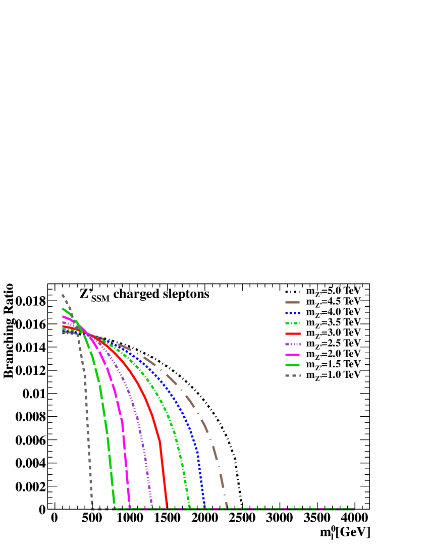
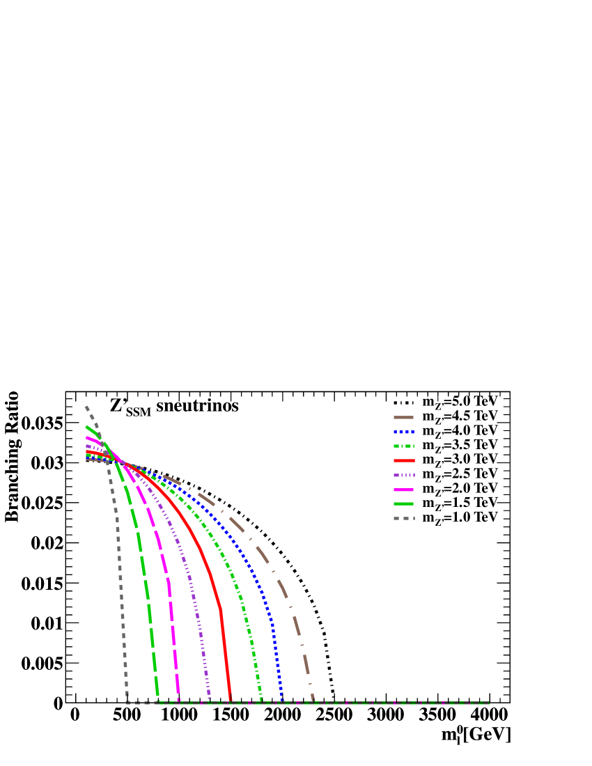
6 Cross sections and event rates at the LHC
In this section we present the total cross section for production at the LHC according to the models discussed throughout this paper, i.e. Table 1, as well as the Sequential Standard Model. We consider collisions at three centre-of-mass energies: 7 TeV (the 2011 LHC run), 8 TeV (the 2012 run) and 14 TeV, the ultimate project energy. For each energy we shall calculate the cross section and estimate the expected number of events with a boson decaying into supersymmetric particles, for a few values of integrated luminosity.
6.1 Leading order production cross section
The cross sections are computed at leading order (LO), employing the LO parton distribution functions CTEQ6L [41] and setting the factorization scale equal to the mass. Using a different LO PDF has a negligible impact on the results. The cross section for Drell–Yan like processes has been computed up to next-to-next-to leading order (NNLO) in QCD and, in principle, the calculations carried out in Refs. [42, 43] can be easily extended to production processes. However, since all partial widths and branching ratios have been evaluated at LO, for the sake of consistency, we decided to stick to the lowest-level approximation.
The parton-level process is analogous to production, i.e. it is the purely SM quark-antiquark annihilation . Since the coupling of the to the quarks depends on the specific scenario, the production rate is a function of the mixing angle and of the mass, but is independent of the MSSM parameters. In the Sequential Standard Model, the cross section just depends on the mass of the . Figures 21–23 present the total cross section for the different models investigated throughout this work, as a function of , at the energies of 7 TeV (Fig. 21), 8 TeV (Fig. 22) and 14 TeV (Fig. 23). For each centre-of-mass energy, we present the results on linear (left) and logarithmic (right) scales. Tables 21, 22 and 23 quote the numerical values of the LO production cross section, varying from 1 to 5 TeV, with steps of 500 GeV, in models and in the Sequential Standard Model.
The highest production cross section is given by the SSM, whereas the model yields the lowest rate; the predictions of the other models lie between these results and are almost indistinguishable for large . Moreover, the rates decrease by several orders of magnitude once increases. In detail, at TeV, the SSM cross section runs from 1.6 pb ( TeV) to pb ( TeV). The production rate for the -based varies from to pb in the same range, with very little differences among the models. At the centre-of-mass energy of 8 TeV, the variation is between 2.3 pb ( at TeV) and pb (all other models at 5 TeV). At TeV, for a mass of 1 TeV the cross section varies from about 8 pb () to 1.8 pb (); for TeV, all models yield a rate around pb.
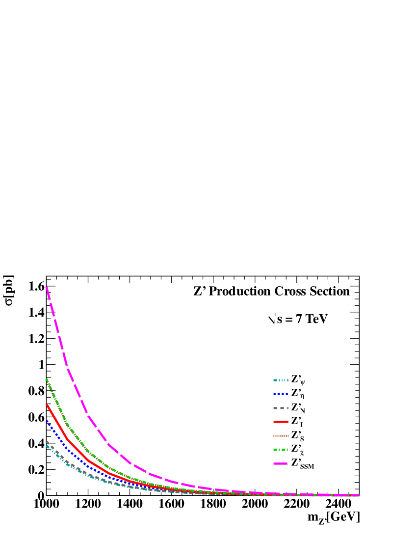
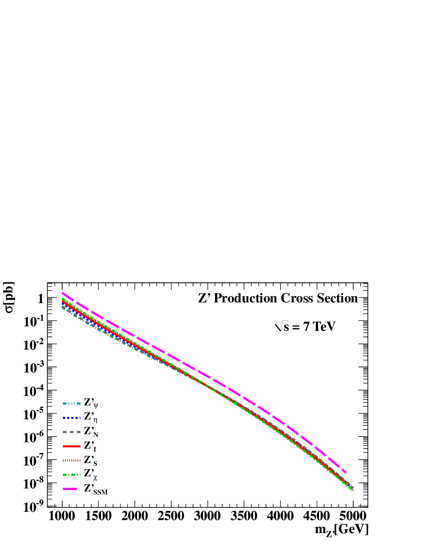
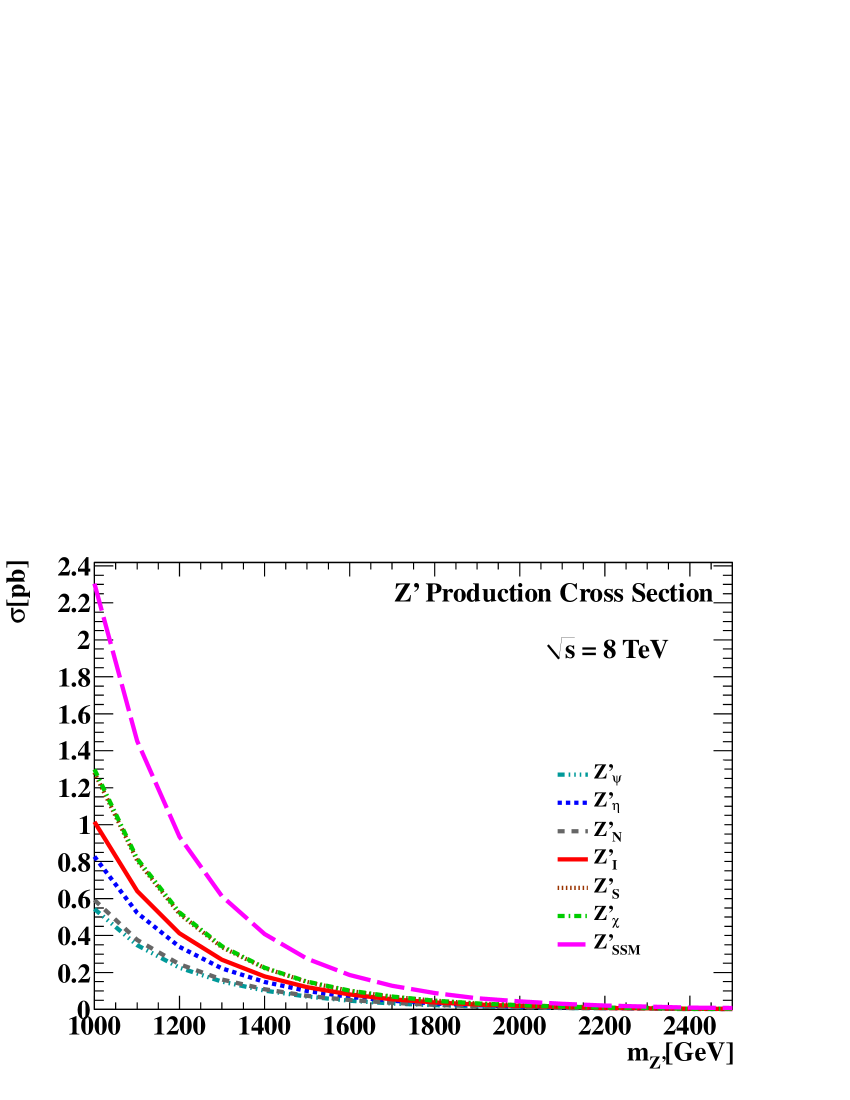
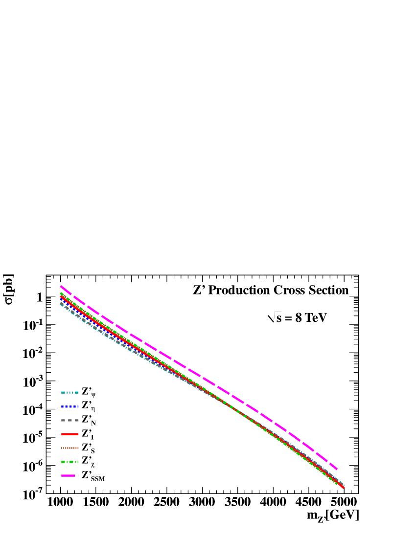
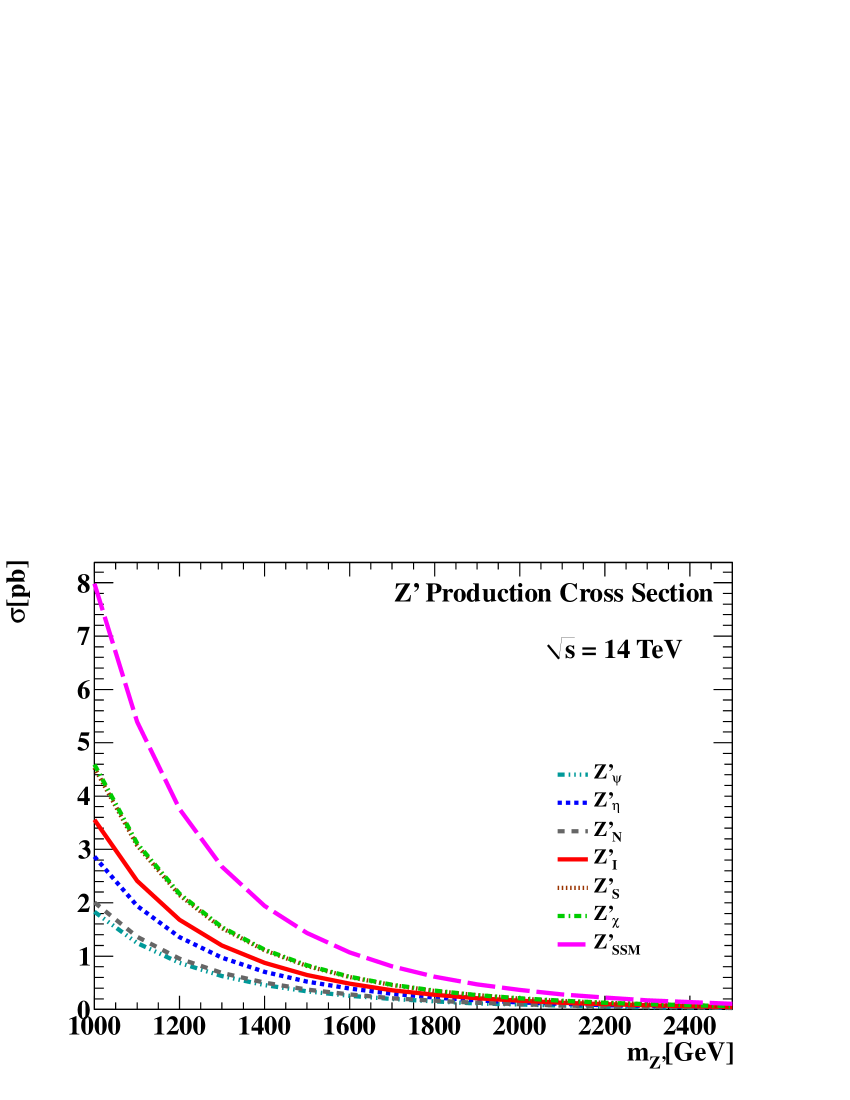
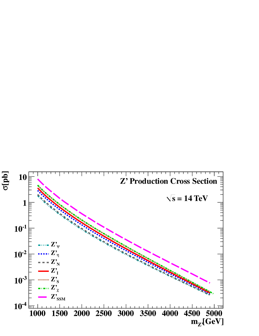
| 1.0 | 0.57 | 0.38 | 0.41 | 0.70 | 0.88 | 0.89 | 1.59 |
| 1.5 | 0.16 | ||||||
| 2.0 | |||||||
| 2.5 | |||||||
| 3.0 | |||||||
| 3.5 | |||||||
| 4.0 | |||||||
| 4.5 | |||||||
| 5.0 |
| 1.0 | 0.83 | 0.54 | 1.01 | 1.28 | 1.28 | 1.30 | 2.30 |
| 1.5 | 0.27 | ||||||
| 2.0 | |||||||
| 2.5 | |||||||
| 3.0 | |||||||
| 3.5 | |||||||
| 4.0 | |||||||
| 4.5 | |||||||
| 5.0 |
6.2 Event rates with sparticle production in decays at the LHC
In the following, we wish to investigate the domain where possible decays into supersymmetric particles could be detectable. For this purpose, we consider two scenarios: =8 TeV, with an integrated luminosity, =20 fb-1, as expected in the 2012 LHC data taking, and, in future perspective, =14 TeV with =100 fb-1. In the narrow-width approximation, the foreseen number of events in decays is simply given by the product of integrated luminosity, production cross section and relevant branching ratio.
The expected event rates in the two considered scenarios are summarized in Tables 24 and 25, for =1.5 and 2 TeV and setting the slepton mass to the values which in Tables 8–20 maximize the slepton rate. We discarded the model as it does not yield a sfermion spectrum after the addition of the D-term to squark and slepton masses. As discussed in Section 5, leptonic final states in supersymmetric events can be yielded by direct decays (Fig. 13) or by a cascade originated from primary decays into sneutrino, chargino or neutralino pairs (see Figs. 14, 15 and 16). By adding up such rates, one obtains the so-called cascade branching ratio:
| (34) |
In Tables 24 and 25 Nslep and Ncasc are the number of events with a decaying into a primary charged-slepton pairs or into a supersymmetric cascade, respectively. In both luminosity (energy) regimes, due to the large cross section, the Sequential Standard Model is the one yielding the highest production of supersymmetric particles in decays, up to - for cascade events at TeV and =100 fb-1 and a mass TeV. As discussed in Sections 5.1 and 5.4, in the and models direct decays into charged sleptons are prevented, but sneutrino, neutralino and chargino productions are accessible, with expected number of events from 50 to according to , energy and integrated luminosity. As for the model, in the high-luminosity phase, a few hundreds of direct sleptons and up to cascade particles can be produced for TeV. For =20 fb-1 and TeV, direct slepton decays are negligible, but about 400 and 70 cascade events can be expected for a mass of 1.5 and 2 TeV, respectively. The boson leads to many cascade particles in the high-luminosity regime, between and , and a few tenths of direct leptons. For the lower-luminosity case, there are no directly produced charged sleptons, whereas the cascade sparticles are about 30 (=1.5 TeV) and 46 ( TeV).
Before concluding this subsection, we point out that, although the numbers in Tables 24 and 25 encourage optimistic predictions on decays into sparticles, especially in the high-luminosity phase, before drawing a conclusive statement on this issue, it will be necessary carrying out a careful study accounting for detector acceptance and resolution, triggering efficiency and cuts on final-state jets and leptons. Hence, the results presented in this paper should be seen a first step towards a more thorough investigation, which requires, above all, the implementation of the models herein discussed into a Monte Carlo event generator. In this perspective, one should compare the Monte Carlo predictions with the experimental data following, e.g., the approach proposed in [44] or investigating the observables suggested in [45] to search for new physics in Drell–Yan like events mediated by a new heavy resonance. The same analysis should be also performed for the Standard Model backgrounds: as discussed in the Introduction, we shall defer the implementation of the modelling for production and decays, as well as the comparison with the simulation of the backgrounds, to future work.
| Model | Ncasc | Nslep | |
|---|---|---|---|
| 1.5 | 523 | – | |
| 2 | 55 | – | |
| 1.5 | 599 | 36 | |
| 2 | 73 | 4 | |
| 1.5 | 400 | 17 | |
| 2 | 70 | 3 | |
| 1.5 | 317 | – | |
| 2 | 50 | – | |
| 1.5 | 30 | – | |
| 2 | 46 | – | |
| 1.5 | 2968 | 95 | |
| 2 | 462 | 14 |
| Model | Ncasc | Nslep | |
|---|---|---|---|
| 1.5 | 13650 | – | |
| 2.0 | 2344 | – | |
| 1.5 | 10241 | 622 | |
| 2.0 | 2784 | 162 | |
| 1.5 | 9979 | 414 | |
| 2.0 | 2705 | 104 | |
| 1.5 | 8507 | – | |
| 2.0 | 2230 | – | |
| 1.5 | 8242 | 65 | |
| 2.0 | 2146 | 16 | |
| 1.5 | 775715 | 24774 | |
| 2 | 19570 | 606 |
7 Conclusions
In this paper, we discussed production and decay of new neutral bosons, according to new physics models based on a gauge group and in the Sequential Standard Model. Unlike most analyses undertaken so far, based on SM decays, we also included supersymmetric decay modes, as predicted by the Minimal Supersymmetric Standard Model: in this perspective, the current mass limits may have to be revisited. Extending the MSSM with the symmetry implies new features, such as an extra scalar neutral Higgs boson, two novel neutralinos and a modification of the sfermion masses due to an additional contribution to the so-called D-term. The particle mass spectra were studied in terms of the parameters characterizing the group and the MSSM; in particular, we discarded scenarios wherein, for fixed values of the sfermion soft mass, squarks or sleptons are not physical after the addition of the D-term. The same study has been performed for the purpose of the partial widths and branching ratios, paying special attention to final states with charged leptons and missing energy. In fact, these configurations are favourable for an experimental detection at hadron colliders and can be yielded by intermediate charged sleptons or a supersymmetric cascade through neutralinos, chargino and sneutrinos. The branching ratios of these decays have been investigated in all the models, as a function of the slepton mass.
We finally computed the production LO cross section in all scenarios and gave an estimate of the number of supersymmetric events in decays, in the narrow-width approximation and for few values of centre-of-mass energy and integrated luminosity. The outcome of this study is that, for some models and parametrizations, one can even have up to - events with sparticle production in decays. As an additional remark, we wish to point out that the decay presents two interesting features. First, the mass will set an additional constrain on the slepton invariant mass; second, it allows the exploration of corners of the phase space which would be instead unaccessible through other processes, e.g. Drell–Yan like events.
In summary, we consider our investigation a useful starting point to study production and decay beyond the Standard Model, such as within supersymmetric theories, drawing guidelines for future experimental analyses. In future perspective, it will be very interesting performing a study including parton showers, finite-width and hadronization corrections, as well as experimental effects, like the detector simulation and the acceptance cuts. In this way, one will eventually be able to draw a statement on the mass limits within supersymmetry. To reach these objectives, the models for production and decay, examined throughout this paper, will have to be implemented in Monte Carlo programs, such as HERWIG or PYTHIA, and the supersymmetry signals compared with the Standard Model backgrounds simulated, e.g., by means of the ALPGEN code [46]. In the framework of an event generator, it will also be possible, in the same manner as the experimental analyses do, rescaling the total cross section in such a way to include higher-order QCD corrections. For this purpose, the use of the FEWZ code [47], which simulates vector boson production at hadron colliders at NNLO, with fully exclusive final states, is planned. Other possible extensions of our analysis consist in investigating more thoroughly the unconventional assignment of the SM and exotic fields to the SU(10) representations, as well as scenarios wherein the exotic leptons (sleptons) and quarks (squarks), predicted by the grand-unified group E6, but discarded in the present work, are lighter than the and therefore capable of contributing to its decay width. This is in progress.
8 Acknowledgements
We are especially indebted to T. Gherghetta for a very useful correspondence aiming at understanding the results and the modelling of Ref. [12]. We acknowledge R. Barbieri, M.L. Mangano, B. Mele, E. Nardi and M.H. Seymour for discussions on these and related topics. We are grateful to V. Sanz, who pointed out a mistake in a Feynman diagram presented in the previous versions of this paper.
Appendix A decay rates into standard and supersymmetric particles
The Lagrangian term describing the interaction of the with fermions is given by:
| (35) |
with
| (36) |
Setting , the vector and axial-vector couplings read:
| (37) |
where the charges of left- and right-handed fermions can be obtained by using Eq. (12) and Table 2. In terms of the mixing angle , such couplings read:
| (38) |
One can thus write the width into fermion pairs as:
| (39) |
where the colour factor is for quarks and for leptons. With the charges listed in Table 2 and employing Eq. (38), one can show that, in the model, namely , the vector and vector-axial couplings of the with up-type quarks vanish, i.e. . In fact, when discussing phenomenology at the Representative Point (Section 4), it was pointed out that its branching ratio into pairs is null.
Likewise, the interaction Lagrangian of the sfermions with the reads:
| (40) |
The width into left- or right-handed sfermions is given by:
| (41) |
where the sign refers to left- and right-handed sfermions, respectively. Eq. (41) is expressed in terms of weak eigenstates ; its generalization to the mass eigenstates is straightforward and discussed in [12]. However, for the parametrizations used throughout this paper, sfermion mixing is always negligible and Eq. (41) can be safely used even to calculate the branching ratios into and final states.
From Eq. (41) one can learn that the rate into left- and right-handed sfermions vanishes for and , respectively. In fact, for , according to Eq. (35), the only couples to left-handed fermions and therefore in the MSSM, in absence of left-right mixing, there is no coupling with right-handed sfermions. Likewise, for , the only couples to right-handed fermions and sfermions and the rate into pairs is null. For example, in the model, it is , whereas, in the model, . Therefore, as remarked in Sections 5.3 and 5.4, the and are suppressed, although they are kinematically permitted at the Reference Point.
As for the Higgs sector, defining , and the charges as in Eq. (15) and , one can obtain the rate for decays into charged-Higgs pairs [48]
| (42) |
and associated production of a boson with a charged Higgs 999Eq. (43) corrects a typing mistake present in Ref. [12], wherein the decay width is instead 4 times smaller than in (43).
| (43) | |||||
As the has no direct coupling with ’s, the decay into pairs occurs by means of the - mixture. For small values of the - mixing angle, this width reads [48]:
| (44) |
In order to obtain the widths into -Higgs pairs, i.e. , or final states, or into scalar-pseudoscalar neutral-Higgs pairs, such as , or , one first needs to diagonalize the neutral Higgs mass matrix (see [12]). The -Higgs rate can be written in compact form as:
| (45) | |||||
where for final states , and , respectively, and is the matrix which diagonalizes the Higgs mass matrix in the basis. Likewise, using the same notation as in Eq. (45), the scalar-pseudoscalar Higgs width reads:
| (46) | |||||
Finally, one can derive the decay widths into gauginos. As for neutralinos, after diagonalizing the mass matrix (21), the interaction Lagrangian reads:
| (47) |
where is a generalized coupling depending on the diagonalizing-matrix elements and has been calculated numerically. The partial rate into neutralino pairs () with masses and is thus given by:
| (48) | |||||
Finally, the Lagrangian term corresponding to the coupling of the with charginos is given by:
| (49) |
The generalized vector and vector-axial couplings can be expressed in terms of , the angles of the unitary transformation diagonalizing the chargino mass matrix [18], and the Higgs charges as follows [12]:
| (50) |
In the above equations, . The analytical expressions for can be found in [18] and are not reported here for brevity. The rate into chargino pairs is finally given by:
| (51) | |||||
References
- [1] P. Langacker, Rev. Mod. Phys. 81 (2009) 1199.
- [2] J.L. Hewett and T.G. Rizzo, Phys. Rep. 183 (1989) 193.
- [3] E. Salvioni, G. Villadoro and F. Zwirner, JHEP 0911 (2009) 068.
- [4] E. Salvioni, A. Strumia and F. Zwirner, JHEP 1003 (2010) 010.
- [5] CDF Collaboration, Phys. Rev. Lett. 106 (2011) 121801.
- [6] D0 Collaboration, Phys. Lett. B695 (2011) 88.
- [7] ATLAS Collaboration, Phys. Rev. Lett. 107 (2011) 272002; Phys. Lett. B700 (2011) 163.
- [8] CMS Collaboration, JHEP 1105 (2011) 093.
- [9] L. Randall and R. Sundrum, Phys. Rev. Lett. 83 (1999) 4690.
- [10] H. E. Haber and G. L. Kane, Phys. Rep. 117 (1985) 75.
- [11] R. Barbieri, S. Ferrara, and C. A. Savoy, Phys. Lett. B119 (1982) 343.
-
[12]
T. Gherghetta, T. A. Kaeding, and G. L. Kane, Phys. Rev. D57 (1998) 3178.
See also the unpublished version, arXiv:hep-ph/9701343v2, for the complete expressions of mass matrices and decay widths. - [13] J. Kang and P. Langacker, Phys. Rev. D71 (2005) 035014.
- [14] V. Barger, P. Langacker, H.-S. Lee and G. Shaughnessy, Phys. Rev. D73 (2006) 115010.
- [15] V. Barger, P. Langacker and G. Shaughnessy, Phys. Lett. (2007) B644 361.
- [16] M. Baumgart, T. Hartman, C. Kilic and L.-T. Wang, JHEP 0711 (2007) 084.
- [17] C.-F. Chang, K. Cheung and T.-C. Yuan, JHEP 1109 (2011) 058.
- [18] S. P. Martin, ’A Supersymmetry Primer’, in Perspectives on Supersymmetry II, G.L. Kane ed., pp. 1-153,arXiv:hep-ph/9709356.
- [19] B. de Carlos and J. Espinosa, Phys. Lett. B407 (1997) 12.
- [20] J. Kalinowski, S.F. King and J.P. Roberts, JHEP 0901 (2009) 066.
- [21] G. Bélanger, J. Da Silva and A. Pukhov, JCAP 1112 (2011) 014.
-
[22]
G. Corcella et al., JHEP 0101 (2001) 010;
S. Gieseke et al., arXiv:1102.1672 [hep-ph]. - [23] T. Sjostrand, S. Mrenna and P. Skands, JHEP 0605 (2006) 026; Comput. Phys. Commun. 178 (2008) 852.
- [24] J. Erler, P. Langacker and T. Li, Phys. Rev. D66 (2002) 015002.
- [25] E. Nardi, Phys. Rev. D48 (1993) 3277.
- [26] E. Nardi, Phys. Rev. D49 (1994) 4394.
- [27] E. Nardi and T.G. Rizzo, Phys. Rev. D50 (1994) 203.
- [28] R.W. Robinett and J.L. Rosner, Phys. Rev. D25 (1982) 3036; Erratum-ibid. D27 (1983) 679.
- [29] J. Erler, P. Langacker, S. Munir and E. Rojas, JHEP 0908 (2009) 017.
- [30] K.S. Babu, C. Kolda and J. March-Russell, Phys. Rev. D54 (1996) 4635.
- [31] V. Barger and K. Whisnant, Int. J. Mod. Phys. A3 (1988) 1907.
- [32] S. Nandi, Phys. Lett. 197 (1997) 144.
- [33] P. Fayet and J. Iliopoulos, Phys. Lett. B51 (1974) 461.
- [34] L. O’Raifeartaigh, Nucl. Phys. B96 (1975) 331.
- [35] K. Nakamura et al., J. Phys. G37 (2010) 075021.
- [36] ALEPH, DELPHI, L3, OPAL Collaborations, and LEP Working Group for Higgs Boson Searches, Phys. Lett. B565 (2003) 61.
- [37] CDF and D0 Collaborations, Phys. Rev. Lett. 104 (2010) 061802; Phys. Rev. Lett. 109 (2012) 071804.
- [38] ATLAS Collaboration, Phys. Lett. B710 (2012) 49; Phys. Rev. D86 (2012) 032003.
- [39] CMS Collaboration, Phys. Lett. B710 (2012) 26; Phys. Lett. B716 (2012) 30.
- [40] F. E. Paige, S. D. Protopopescu, H. Baer, and X. Tata, hep-ph/0312045.
- [41] J. Pumplin, D.R. Stump, J. Huston, H.L. Lai, P. Nadolsky and W.K. Tung, JHEP 0207 (2002) 012.
- [42] R. Hamberg, W. L. van Neerven and T. Matsuura, Nucl. Phys. B359 (1991) 343; Erratum-ibid. B644 (2002) 403.
- [43] R. V. Harlander and W. B. Kilgore, Phys. Rev. Lett. 88 (2002) 201801.
- [44] J. Erler, P. Langacker, S. Munir and E. Rojas, JHEP 1111 (2011) 076.
- [45] C.-W. Chiang, N.D. Christensen, G.-J. Ding and T. Han, Phys. Rev. D85 (2012) 015023.
- [46] M.L. Mangano, M. Moretti, F. Piccinini, R. Pittau and A. Polosa, JHEP 0307 (2003) 001.
- [47] R. Gavin, Y. Li, F. Petriello and S. Quackenbush, Comput. Phys. Commun. 182 (2011) 2388.
- [48] N.G. Deshpande and J. Trampetic, Phys. Lett. B206 (1988) 665.