Thermodynamic formalism for dissipative quantum walks

Abstract

We consider the dynamical properties of dissipative continuous time quantum walks on directed graphs. Using a large deviation approach we construct a thermodynamic formalism allowing us to define a dynamical order parameter, and to identify transitions between dynamical regimes. For a particular class of dissipative quantum walks we propose a new quantum generalization of the the classical pagerank vector, used to rank the importance of nodes in a directed graph. We also provide an example where one can characterize the dynamical transition from an effective classical random walk to a dissipative quantum walk as a thermodynamic crossover between distinct dynamical regimes.

I Introduction

For a system in thermodynamic equilibrium Statistical Mechanics and Thermodynamics provide the formalism to characterize different phases of matter, and the transitions from one phase to another Hill and Physics (1987). Quantum fluctuations alone can give origin, at zero temperature, to quantum phase transitions Sachdev (2011) whose effects can experimentally be observed in a critical region at small but finite temperatures. Away from thermodynamic equilibrium engineered open quantum systems provide a more recent source of interest Verstraete et al. (2009); Diehl et al. (2008); Kraus et al. (2008). In these latter settings a controlled environment can be used to drive the system to a steady state whose properties depend on system and environment parameters. This approach has been used to study dissipative phase transitions controlled by the coupling constants in the equation of motion Diehl et al. (2010), and to formulate a dissipative model of quantum computation Verstraete et al. (2009).

Most of the research on quantum dissipative systems focuses on the static properties of the steady state, in this work we adopt a different dynamical perspective, where the time parameter plays a more explicit role in characterizing the system. This allows us to study the occurrence of dynamical crossovers or dynamical phase transitions driven by fluctuations in the ensemble of possible evolutions. The model systems that we consider, of relevance both to quantum computation and condensed matter, are dissipative Continuous Time Quantum Walks (CTQWs). The standard CTQWs (the unitary analog of classical random walks) describe the coherent motion of an excitation on the vertices of an undirected graph Aharonov et al. (2001); Farhi and Gutmann (1998); Childs et al. (2002); Farhi et al. (2008). They are a powerful tool in quantum computation, providing a useful approach to algorithms’ design, and an alternative framework for universal quantum computation Childs (2009). More recently CTQWs have also been used to describe transport properties in complex networks Mulken and Blumen (2011); Tsomokos (2011), while dissipative CTQWs have found applications in the context of quantum biologyRebentrost et al. (2009a); Mohseni et al. (2008); Plenio and Huelga (2008); Caruso et al. (2009); Rebentrost et al. (2009b); Giorda et al. (2011), and quantum state transfer in superconducting qubits Strauch (2009); Strauch and Williams (2008).

In this work, following Whitfield et al. (2010), we will refer to dissipative CTQWs as Quantum Stochastic Walks (QSWs). Using the quantum jump approach Plenio and Knight (1997) we study the statistical properties of the ensemble of trajectories originated by QSWs. The mathematical tool allowing us to probe the dynamics of the system and the structure of the space of trajectories is known as Large Deviation (LD) theory Touchette (2009). The latter finds applications in different areas of statistical mechanics and computer science (see Touchette (2009) and references therein). Using the LD approach it is possible to construct a formalism, for the ensemble of possible evolutions, resembling standard thermodynamics. Since the LD theory overlaps with the thermodynamic formalism developed by Ruelle and others Ruelle (2004) in the context of chaos theory and dynamical systems, in the following we will use the expressions thermodynamic formalism and LD approach interchangeably.

From the application of the thermodynamic formalism to QSWs we obtain two main results: first, a quantum generalization of the pagerank vector Brin and Page (1998); Langville and Meyer (2006), a measure used to rank the importance of nodes in a graph; second, a tool to study transitions from classical to quantum dissipative dynamical regimes from a thermodynamic point of view (see Shikano (2011) for a different approach). In particular, we provide an instance of a simple QSW presenting a dynamical crossover between the two regimes.

The rest of the paper is divided as follows: in the second section we define the notion of QSW as introduced in Whitfield et al. (2010); in the third section we provide a brief introduction to the LD approach; in the fourth section we apply the thermodynamic formalism to describe the dynamics of a QSW on a directed graphs; while the last section is devoted to discussions and conclusions.

II Quantum stochastic walks

QSWs are a class of stochastic processes introduced in Whitfield et al. (2010) with the purpose of generalizing both continuous time quantum walks, and classical random walks Venegas-Andraca (2008) into a single framework. A QSW is specified by a quantum master equation in Lindblad form Breuer and Petruccione (2002) describing the evolution of the system’s density matrix

$$\dot{\rho}=-i[H,\rho]+\sum_{k=1}^{N_{L}}L_{k}\rho L_{k}^{\dagger}-\frac{1}{2}\{L_{k}^{\dagger}L_{k},\rho\},$$ (1)

where $[\cdot,\cdot]$ and $\{\cdot,\cdot\}$ stand respectively for the commutator and the anticommutator, and the operators $L_{k}$ are called jump operators. The dynamics described by eq. 1 is characterized by the interplay between a coherent part associated to $H$, and an incoherent part associated to the jump operators $\{L_{k}\}$. If only the coherent term was present the QSW would correspond to a standard CTQW. On the other hand, it can be shown that if only the incoherent term was present the QSW would correspond to a classical random walk for the diagonal elements of $\rho(t)$ Whitfield et al. (2010).

A standard stochastic method to study the dynamics described by eq. 1 is provided by the quantum jump approach Plenio and Knight (1997); Breuer and Petruccione (2002). In this framework one considers an ensemble of piecewise deterministic evolutions of pure states $\{|\psi_{\alpha}(t)\rangle\}$ (where $\alpha$ labels an element in the ensemble). The average over different trajectories (or histories) provides the state of the system at each instant of time

$$\rho(t)=\left[|\psi_{\alpha}(t)\rangle\langle\psi_{\alpha}(t)|\right]_{\rm ave}\equiv\sum_{\alpha=1}^{N_{\alpha}}\frac{|\psi_{\alpha}(t)\rangle\langle\psi_{\alpha}(t)|}{N_{\alpha}}.$$ (2)

The dynamics of each pure state evolves deterministically for some time-interval according to the following non-hermitian effective Hamiltonian

$$H_{\rm eff}\equiv H-i\sum_{k=1}^{N_{L}}\frac{1}{2}L_{k}^{\dagger}L_{k}.$$ (3)

The deterministic evolution is interrupted at certain random times $\tau$ by a quantum jump operator $L_{k}$, which projects the state according to

$$|\psi(\tau)\rangle\rightarrow\frac{L_{k}|\psi(\tau)\rangle}{\|L_{k}|\psi(\tau)\rangle\|_{2}}.$$ (4)

In between random jumps the state evolves according to $H_{\rm eff}$. The use of an ensemble of quantum trajectories associated to the QSW in eq. 1 is also referred to as the stochastic unraveling of the quantum master equation. More details on this method can be found in Plenio and Knight (1997); Breuer and Petruccione (2002).

Since the quantum walker evolves on a graph we also need to specify how the graph’s structure enters into eq. 1. A natural way to proceed is to use the set of multi-indices $\{(i,j)\}$ (where $i$ and $j$ are the nodes of the graph) to label the index $k$ in $L_{k}$

$$L_{k}\rightarrow L_{ij}\equiv M_{ij}|i\rangle\langle j|,$$ (5)

and the matrix $M$ contains the rate coefficients of the jumps from $|j\rangle$ to $|i\rangle$, in the site basis. This way the quantum jump in eq. 4 corresponds to hopping from one site to another at a rate given by $M$. For the coherent part of the evolution the Hamiltonian $H$ in eq. 1 is identified with the adjacency matrix of the graph with all directions removed, so that $H$ is a symmetric matrix. Note that only the dissipative part in the master equation is the one that encodes for the direction of the edges. In the next section we introduce the thermodynamic formalism used to study the evolution of a QSW.

III Large deviation theory and thermodynamic formalism

The dynamics of a stochastic system provides many useful information that cannot be accessed from the knowledge of the stationary state alone. The large deviation approach is the mathematical framework allowing us to access this extra information Touchette (2009). In fact, recently, its application to classical and quantum nonequilibrium dynamics has being crucial to show the presence of dynamical phase transitions and dynamical crossover phenomena Hedges et al. (2009); Garrahan and Lesanovsky (2010); Garrahan et al. (2007). In particular, as first observed in Garrahan and Lesanovsky (2010), the quantum jump approach provides a quantum stochastic process that is well suited to be analysed with the LD theory. In what follows we show how to adapt the method developed in Garrahan and Lesanovsky (2010) to the context of QSWs.

Given a quantum stochastic walker evolving according to eq. 1, we are interested in the time record of jump events associated to one or more operators $L_{k}$. In the quantum jump approach this record is one particular realization of a quantum trajectory. Introducing a variable $K$, which counts the number of events (or jumps) up to a certain time for a particular jump operator, we define the probability

$$p(K,t)\equiv{\rm Tr}[\rho(K,t)],$$ (6)

corresponding to the observation of a number $K$ of events up to time $t$. $\rho(K,t)$ is the density matrix of the system conditioned on the observation of those $K$ events. The probability generating function of the distribution $p(K,t)$ is given by

$$Z(s,t)\equiv\sum_{K=0}^{\infty}e^{-sK}p(K,t)={\rm Tr}\sum_{K=0}^{\infty}e^{-sK}\rho(K,t).$$ (7)

We define the auxiliary operator $\rho(s,t)$ as the Laplace transform of $\rho(K,t)$

$$\rho(s,t)\equiv\sum_{K=0}^{\infty}e^{-sK}\rho(K,t).$$ (8)

The long time behavior of the generating function $Z$ has the following large deviation form

$$Z(s,t)\approx e^{t\theta(s)}.$$ (9)

The reason why this is the case will be more clear when we consider the dynamics of $\rho(s,t)$ in the limit $t\rightarrow\infty$. Equation 9 defines the function $\theta$ which, in this formalism, is the analogue of a thermodynamic free-energy density, while $s$ is interpreted as an intensive thermodynamic variable (the analogue of a chemical potential for example), conjugate to the counting variable $K$, and the time parameter plays the role of a volume. The function $\theta$ is the fundamental object characterizing the dynamics of the process in terms of thermodynamic properties in the space of stochastic trajectories (the ensemble of possible time records for the counting variable $K$). Note that it is possible to consider not just one, but instead a set of jump processes associated to the jump operators $\{L_{k_{i}}\}$, and correspondingly a set of counting variables $\{K_{i}\}$ can be taken into account. Accordingly one can introduce different intensive parameters $\{s_{i}\}$, conjugated to $\{K_{i}\}$. Since in the following we associate one counting variable to each node of a graph, we use the vector notation for the variables $\vec{s}$ and $\vec{K}$.

The dynamical free-energy $\theta$ can be obtained from the diagonalization of a generalized Liouville superoperator describing the dynamics of the auxiliary operator $\rho(\vec{s},t)$. As shown in appendix A the Laplace transform in eq. 8 decouples the evolution of $\rho(\vec{K},t)$ for different vectors $\vec{K}$, and this allows us to derive the following generalized quantum master equation for the auxiliary operator

$$\dot{\rho}(\vec{s},t)=\mathbb{W}_{\vec{s}}[\rho(\vec{s},t)]\equiv\mathbb{L}[\rho({\vec{s}},t)]+\mathbb{V}_{\vec{s}}[\rho(\vec{s},t)].$$ (10)

$\mathbb{L}$ is the same Liouville superoperator as in eq. 1

$$\mathbb{L}[\cdot]=-i[H,\cdot]+\sum_{k=1}^{N_{L}}L_{k}\cdot L_{k}^{\dagger}-\frac{1}{2}\{L_{k}^{\dagger}L_{k},\cdot\},$$ (11)

while

$$\mathbb{V}_{\vec{s}}[\cdot]=\sum_{d}(e^{-s_{d}}-1)L_{d}\cdot L_{d}^{\dagger},$$ (12)

and $d$ labels elements of a subset of $\{1,...,N_{L}\}$, those associated to the jump processes that we want to track in time. When all the entries of $\vec{s}$ are 0 we recover the real typical dynamics, otherwise $\mathbb{W}_{\vec{s}}$ determines an evolution whose unfolding into trajectories is biased by $e^{-\vec{s}}$. Following Garrahan and Lesanovsky (2010) we call this ensemble of trajectories the $s$-ensemble. In the classical context the analogue of $\mathbb{W}_{\vec{s}}$ is known as the Lebowitz-Spohn operator Lebowitz and Spohn (1999), and the free-energy function $\theta$ is given by the largest real part of its eigenvalues. In the quantum case one can adopt a similar prescription and identify $\theta({\vec{s}})$ with the largest real part of the eigenvalues of $\mathbb{W}_{\vec{s}}$ Garrahan and Lesanovsky (2010), accordingly with eq. 9 and with the fact that for long times the largest real part of the eigenvalues will be the dominant one in evaluating $Z(s,t)$. Once we have associated a dynamical free-energy to the ensemble of quantum trajectories of the system we can consider derivatives of the free-energy function, whose behavior tell us about the presence of dynamical crossovers or dynamical phase transitions. As an example calculation we now derive the form of the first and second derivatives of the dynamic free-energy. Using eqs. 7, 9 and 8 we can write in the long time limit

$$\theta({\vec{s}})=\frac{d}{dt}{\rm Log}\;{\rm Tr}\rho({\vec{s}},t)=\frac{{\rm Tr}\dot{\rho}({\vec{s}},t)}{Z({\vec{s}},t)}.$$ (13)

The numerator in the last expression equals to

$${\rm Tr}\dot{\rho}({\vec{s}},t)={\rm Tr}\mathbb{W}_{\vec{s}}[{\rho}({\vec{s}},t)]={\rm Tr}\mathbb{V}_{\vec{s}}[{\rho}({\vec{s}},t)],$$ (14)

where the last equality follows simply from eq. 1 and the cyclicity property of the trace. Hence we have that

$$\theta({\vec{s}})=\frac{{\rm Tr}\mathbb{V}_{\vec{s}}[\rho(\vec{s},t)]}{Z({\vec{s}},t)}=\sum_{d}(e^{-{{s_{d}}}}-1){\rm Tr}\;L_{d}^{\dagger}L_{d}\tilde{\rho}({\vec{s}},t),$$ (15)

where we have introduced the normalized density matrix

$$\tilde{\rho}({\vec{s}},t)\equiv\frac{\rho({\vec{s}},t)}{Z({\vec{s}},t)}.$$ (16)

Notice that $\theta(0)=0$, consistently with the existence of a steady state for the dynamics described by $\mathbb{L}$. The partial derivative of $\theta$ with respect to $s_{d}$, for a particular $d$, is given by

$$\partial_{d}\theta\equiv\frac{\partial\theta}{\partial s_{d}}=(e^{-s_{d}}-1){\rm Tr}(O_{d}\partial_{d}\tilde{\rho})-e^{-s_{d}}{\rm Tr}(O_{d}\tilde{\rho}),$$ (17)

where $O_{d}\equiv L_{d}^{\dagger}L_{d}$. We now introduce the activity vector parameter $\vec{\alpha}$, given by the inverse of the first derivative of $\theta(\vec{s})$

$$\alpha_{d}\equiv-\partial_{d}\theta.$$ (18)

It is easy to see that, at $s=0$, the activity coincides with ${\rm Tr}[O_{d}{\rho}^{(ss)}]$; ${\rho}^{(ss)}$ being the stationary state associated with $\mathbb{L}$. This means that, at $s=0$, the dynamical activity $\vec{\alpha}$ coincides with the static expectation value of the operator $O_{d}$ in the steady state, so in this case there is a direct correspondence between static and dynamic order parameters. Hence it is not necessary to perform a dynamical analysis to access the value of the activity at $s=0$. Nevertheless higher order derivatives of the free-energy function, and the behavior of the system at $s\neq 0$ cannot be determined by static quantities. Those are the kind of information that can be accessed only with the LD approach. For a general value of $\vec{s}$ it is easy to show that $t\alpha_{d}=[K_{d}]_{\rm ave}$, in fact

$$\frac{[K_{d}]_{\rm ave}}{t} = \frac{\sum K_{d}e^{-\vec{s}\cdot\vec{K}}p(\vec{K},t)}{tZ}$$ (19)

$$= \frac{-\partial_{d}{\rm Log}Z}{t}=-\partial_{d}\theta=\alpha_{d}.$$

This explains why $\vec{\alpha}$ is named activity: it coincides with the typical number of jump events per unit of time, for a particular value of $\vec{s}$.

The second partial derivative of $\theta$ in the $d$ direction is given by

$$\partial^{2}_{d}\theta = e^{-s_{d}}{\rm Tr}(O_{d}\tilde{\rho})-2e^{-s_{d}}{\rm Tr}(O_{d}\partial_{d}\tilde{\rho})$$ (20)

$$+(e^{-s_{d}}-1){\rm Tr}(O_{d}\partial_{d}^{2}\tilde{\rho}).$$

For the second derivative, even at $s=0$, one does not have a correspondence to any purely static observable. A useful quantity to look at in order to estimate the fluctuations in time of the local activity is provided by the index of dispersion

$$\delta_{d}(s)\equiv-\frac{\partial^{2}_{d}\theta(s)}{\partial_{d}\theta(s)},$$ (21)

the ratio between the variance and the mean of the counting variable $K$ for a particular jump process. In the next section we apply the above formalism in the context of dissipative continuous time quantum walks.

IV Quantum stochastic dynamics on directed graphs

In this section we study the dynamical properties of a QSW on a directed graph using the thermodynamic formalism. In particular, we consider the QSW that has been introduced in Sánchez-Burillo et al. (2012) with the purpose of defining a quantum analogue of the classical notion of pagerank Brin and Page (1998). The latter is a particular graph centrality measure, i.e. an estimate of the relative importance of a node in a graph with respect to the dynamic of a random walker on the graph. Following Sánchez-Burillo et al. (2012) we consider the quantum master equation given by

$$\dot{\rho}=-i[H,\rho]+\sum_{k=1}^{N_{L}}L_{ij}\rho L_{ij}^{\dagger}-\frac{1}{2}\{L_{ij}^{\dagger}L_{ij},\rho\},$$ (22)

where, in particular, $H$ is the adjacency matrix of the graph obtained by removing the directions on the edges, and the jump operators are defined by

$$L_{ij}\equiv\sqrt{G_{ij}}|i\rangle\langle j|.$$ (23)

The matrix $G$, called Google matrix, is a stochastic matrix associated to an irreducible and aperiodic classical random walk on the graph (for a precise definition of the Google matrix see (Langville and Meyer, 2006)). As shown in Sánchez-Burillo et al. (2012), using a theorem by Spohn Spohn (1977) it is possible to prove that the dynamics described by eq. 22 is relaxing, i.e. that the stationary state is unique. The classical random walk described by the stochastic matrix $G$ also has the same property, and its stationary state is called pagerank, denoted with $\vec{\pi}$. Notice that, without the coherent part given by $H$, the dynamics for the diagonal elements of $\rho(t)$ provided by eq. 22 is identical to the classical random walk described by the Google matrix, and in particular its stationary state coincides with the classical pagerank Sánchez-Burillo et al. (2012). On the other hand, adding the coherent term $H$ modifies the dynamics and the stationary state, allowing for a quantum generalization of the pagerank vector. We are now going to use the thermodynamic formalism to detail the differences between the purely classical and the more general quantum open dynamics.

We start calculating the value of the activity at $s=0$ for the set of jump operators $\{L_{ij};\;j=1,...,n\}$, associated to a chosen node $i$. Using eqs. 17 and 23 we have

$$\alpha_{i}(0)=\sum_{j}G_{ij}{\rm Tr}[|j\rangle\langle j|\rho^{(ss)})=\sum_{j}G_{ij}\rho_{jj}^{(ss)}.$$ (24)

This equation tells us that the activity at $s=0$ is related in a simple way to the diagonal entries of the steady state, through the stochastic matrix $G$. Without the presence of the Hamiltonian $H$ in eq. 22 we would have that $\rho^{(ss)}$ is equal to ${\rm diag}(\pi_{1},\dots,\pi_{n})$, hence

$$\alpha_{i}(0)=\sum_{j}G_{ij}\rho_{jj}^{(ss)}=\sum_{j}G_{ij}\pi_{j}=\pi_{i},$$ (25)

where the last equality follows from the definition of the pagerank vector, the stationary state of $G$. This result is simply a check of the consistency of the thermodynamic formalism applied to the classical pagerank, and it states that at long times the probability of finding the walker in the $i$-th node is equal to the average number of times the walker hits the $i$-th node. It is interesting to observe that the quantum case is different. When the coherent term $H$ is present the stationary state is different from the mixed classical state associated to the pagerank vector: $\rho^{(ss)}\neq{\rm diag}(\pi_{1},\dots,\pi_{n})$. Hence the equation

$$\alpha_{i}(0)=\sum_{j}G_{ij}\rho_{jj}^{(ss)}$$ (26)

defines a dynamical quantum analogue of the classical pagerank given by $\vec{\alpha}$, which is different from the static quantum pagerank $\rho^{(ss)}$ of Sánchez-Burillo et al. (2012). The values provided by $\vec{\alpha}$ quantify the typical number of times the walker jumps into a particular node in the long time limit. On the other hand $\rho^{(ss)}$ provides the probability of finding the walker at a particular node. While a purely classical dynamics would not distinguish between the two quantities, as shown by eq. 26, the quantum dissipative dynamics does differentiate the two because of the coherences (off-diagonal elements) present in the steady state.

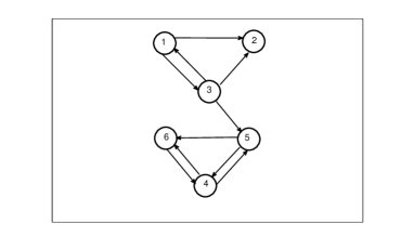
Figure 1: The directed graph that we consider as an example for the application of the thermodynamic formalism to QSWs.

We consider now, as an example, the QSW on the directed graph shown in fig. 1. We set the dimension of the vector $\vec{s}$ to be equal to the size of the graph and, in order to simplify the discussion, we choose all the entries of $\vec{s}$ equal to the same parameter $s$. A similar analysis for a simpler 2-node directed graph can be found in appendix B. The dynamical free-energy $\theta$ is plotted in fig. 2, where one can see that it is equal to 0 at $s=0$, consistently with the fact that the physical dynamic is relaxing, given that $\theta$ is the largest real eigenvalue of $\mathbb{W}_{s}$ in eq. 10.

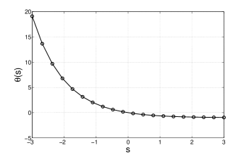
Figure 2: The dynamical free-energy $\theta(s)$ for the QSW associated to the graph in fig. 1.

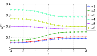
Figure 3: (color online) The normalized dynamical activity of the six nodes of the graph in fig. 1. For this particular example the ranking provided by the activity order parameter does not change as a function of $s$ (see text for more details).

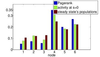
Figure 4: (color online) A comparison between the classical pagerank (left bars), the dynamical activity at $s=0$ (middle bars), and the populations in the steady state (right bars). These values are obtained with respect to the graph shown in fig. 1. Note that the extreme left values in the plot correspond to the classical pagerank.

More interesting is the behavior of the first two partial derivatives of the free-energy function. In fig. 3 we plot the normalized activity with respect to different sites

$$\alpha_{i}^{(n)}\equiv\frac{\alpha_{i}(\vec{s})}{\sum_{i=1}^{6}\alpha_{i}(\vec{s})}.$$ (27)

The figure shows a smooth dynamical crossover from the active region, where large negative values of $s$ favour trajectories with many jumps, to the inactive region, where large positive values of $s$ favour trajectories with few jumps [see eq. 12]. Note that eq. 27 is not well defined in the limit $s\rightarrow\infty$, since in this case one is left with a purely deterministic evolution according to $H_{\rm eff}$ [see eq. 3], which implies $\alpha_{i}(s\rightarrow\infty)=0$. This is not a problem for our approach, since one could always use the unnormalized activity $\vec{\alpha}$, which is well defined for every value of $s$. However the normalized $\vec{\alpha}^{(n)}$ is useful, since it makes the quantitative comparison between the classical pagerank and its quantum dynamical generalization easier. Moreover, in the limit $s\rightarrow-\infty$ the dynamics in eq. 10 is dominated by $\mathbb{V}_{\vec{s}}$, with no time intervals of deterministic evolution. These two extreme scenarios select trajectories that are either associated to “lazy” QSWs which never jumps, or to very active QSWs that are effectively equivalent to the classical random walk described by $G$ (in fact $\vec{\alpha}^{(n)}$ in this limit coincides with the classical pagerank). The transition between the two extreme ensembles of trajectories is controlled by the parameter $s$. For the particular example that we consider the activity ranking (the sorted list of the elements in the vector $\vec{\alpha}$) is preserved for all values of $s$, so in particular it coincides with the classical ranking provided by $\vec{\pi}$, as shown in fig. 3. However the specific values of the activity ranking is a function of $s$, and it could be the case that particular graphs show some rank crossings as $s$ is changed. We note that the situation is different if one considers the quantum ranking provided by the population (the occupation probability) at each node in the steady state Sánchez-Burillo et al. (2012). As shown in fig. 4 the population ranking is different for nodes 2 and 3, with respect to the classical pagerank and the activity ranking. This simple example shows a peculiar aspect of QSWs with respect to classical random walks, i.e. their richer dynamical behavior translates in distinguishable ways of estimating nodes’ centralities.

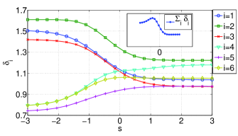
Figure 5: (color online) The stability parameter quantifying fluctuations in the trajectories for different values of $s$. Each line corresponds to a node in the graph of fig. 1. The inset shows the sum with respect to all nodes of the same quantities, and it shows a maximum close to $s=-1$.

We now look at the dynamical fluctuations of the counting processes. In fig. 5 we plot $\delta_{i}$ [see eq. 21] with respect to different nodes. As we said before $\delta_{i}$ is a measure of the dispersion of the counting variable with respect to its average value, and it provides information on the fluctuations in time of the stochastic process. In particular for $\delta_{i}>1$ the process is said to be over-dispersed, meaning that the jumps are clustered in time, having time windows with many jumps, and time windows with almost no jumps. On the other hand, if $\delta_{i}<1$ the process is under-dispersed, meaning that the jump events are more uniformly distributed in time. The dynamical index of dispersion $\delta_{i}$ can itself provide a centrality measure for the $i$-th node, quantifying the stability (or robustness) of the activity index with respect to fluctuations: the smaller $\delta_{i}$, the smaller are the fluctuations in time of $\alpha_{i}$. Similarly one can introduce a global index of dispersion: $\delta\equiv\sum_{i}\delta_{i}$, quantifying the fluctuations at the level of the whole network. In fig. 5 one can see a crossover in the dynamical robustness from the active region (associated to an effectively classical dynamics), to the inactive region. Comparing the two extreme behaviours one notices a remarkable difference in terms of dynamical fluctuations of the local activities. In the classical regime the top 3 ranked nodes are also the more stable, while the lowest 3 are over-dispersed. In the quantum regime this is not the case anymore, and all the nodes fluctuates with more similar intensities. In general their stability ranking is strongly dependent on $s$ in a region approximately delimited by $s=-2$ and $s=0$. The inset in the same figure shows the total index of dispersion, i.e. the sum of all site’s indexes, which measures the global dynamical fluctuations. It is interesting to observe that in the transition from classical trajectories to quantum trajectories the behavior of the total dispersion is not monotonic, and it shows a maximum close to $s=-1$ in the active region. The maximum in the global index of dispersion supports the interpretation of a thermodynamic crossover from an effectively classical to a quantum regime in the space of trajectories. This can be seen more clearly in fig. 6, where we plot the relation between the drop in the normalized activity of the 4th sites (the most active), and the global dispersion index. From the figure one can identify two distinct values of the activity order parameter, corresponding to distinguished dynamical phases, together with an increase in dynamical fluctuations in the region separating the two, which includes the physically relevant point $s=0$. In fig. 5 one can see that the stability ranking is highly dependent on $s$ around $0$, which implies that small fluctuations in the dynamical trajectories will have a noticeable effect on $\vec{\delta}_{i}$.

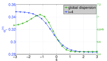
Figure 6: (color online) The figure shows the activity order parameter for the 4-th node in the graph of fig. 1 (triangles), and the total fluctuations of the dynamical trajectories on the same graph (circles). The presence of a maximum in the fluctuations corresponding to the region where the dynamical order parameter is changing is an indication of a crossover phenomenon.

V Conclusions and outlook

In conclusion, we have applied the large deviation approach to study the dynamics of quantum stochastic walks, a particular case of dissipative quantum evolution on directed graphs. The LD approach allows one to formulate a thermodynamic formalism describing quantum dissipative evolutions. We find that the properties of the ensemble of dynamical trajectories of the quantum walker can be used to characterize the structure of the underlying graph. We introduce two new quantum centrality measures Boccaletti et al. (2006), the activity rank and the stability rank. These measures are of relevance in the context of complex networks theory Barrat et al. (2008); Barabási (2002, 2005), providing another connection between complex networks and quantum information theory Giraud et al. (2005); Braunstein et al. (2006); Kimble (2008); Lapeyre et al. (2009); Perseguers et al. (2010a); Perseguers (2010); Perseguers et al. (2010b); Anand et al. (2011); Wu and Zhu (2011); Cuquet and Calsamiglia (2011); Ionicioiu and Spiller (2012); Garnerone et al. (2012a); Paparo and Martin-Delgado (2012); Garnerone et al. (2012b); Sánchez-Burillo et al. (2012); Adhikari et al. (2012). Another interesting aspect of the thermodynamic approach to dissipative quantum walks is the possibility to frame dynamical phases of the evolution in the standard language of Statistical Mechanics and Thermodynamics. We provide an example showing that, already on a small directed graph, the quantum walker displays two dynamical regimes separated by a smooth thermodynamic crossover. Note that this approach is valid also for undirected graphs, though in this case the identification of the most relevant nodes can be simply done looking at the degree distribution: the higher the degree of a node, the higher will be its classical or quantum centrality measure; while the information related to fluctuations around the typical values is less trivial, and it can be obtained with the LD approach.

It would be of interest to understand the connections between the topology of the underlying graph and the dynamical phase space of the quantum dissipative process. The comparison between the simple case of a two-node graph provided in appendix B –where no crossover is present– and the more structured graph in fig. 1, suggests that the topology of the underlying graph can be responsible for the occurrence of different dynamical phases. In particular, exploring more complex graph structures, one could characterize the cases where the transition is sharp (as found in other physical contexts (Garrahan et al., 2007; Hedges et al., 2009; Garrahan and Lesanovsky, 2010)), which would imply a dynamical phase transition between effectively classical and quantum coherent regimes.

Appendix A Derivation of the generalized quantum master equation

We denote with

$$\vec{K}\equiv[K_{1},\dots,K_{i},\dots,K_{l}]$$ (28)

the vector corresponding to the occurrence, up to a certain time, of a number of $K_{i}$ events associated to the jump processes described by $L_{i}$: $K_{1}$ jumps associated to $L_{1}$, $K_{2}$ jumps associated to $L_{2}$ , and so on. The probability at time $t$ for the set of events $\vec{K}$ to occur is given by

$$p(\vec{K};t)\equiv{\rm Tr}\rho(\vec{K};t),$$ (29)

and $\rho(\vec{K};t)$ is the reduced density matrix of the system conditioned on the observation of the set $\vec{K}$ of events. We define the generating function $Z$ as follows

$$Z(\vec{s};t)\equiv\sum_{K_{1},\dots,K_{l}=0}^{\infty}e^{-\vec{s}\cdot\vec{K}}p(\vec{K};t)={\rm Tr}\rho(\vec{s};t),$$ (30)

where

$$\rho(\vec{s};t)\equiv\sum_{\vec{K}}e^{-\vec{s}\cdot\vec{K}}\rho(\vec{K};t).$$ (31)

Using eq. 1 the time evolution of $\rho(\vec{K};t)$, in the $\vec{K}$ sub-manifold, is given by

$$\dot{\rho}(\vec{K};t)=\mathbb{L}_{0}[{\rho}(\vec{K};t)]+\sum_{i}\mathbb{L}_{i}[{\rho}(\vec{K}^{(i)};t)],$$ (32)

with

$$\mathbb{L}_{0}[\cdot] \equiv -i[H,\cdot]-\frac{1}{2}\sum_{i}\{L_{i}^{\dagger}L_{i},\cdot\},$$

$$\mathbb{L}_{i}[{\rho}(\vec{K}^{(i)};t)] \equiv \sum_{i}L_{i}{\rho}(K_{1},\dots,K_{i}-1,\dots,K_{l};t)L_{i}^{\dagger}.$$

It follows that the generalized quantum master equation for $\rho(\vec{s};t)$ is given by

$$\dot{\rho}(\vec{s};t)=\sum_{\vec{K}}e^{-\vec{s}\cdot\vec{K}}\dot{\rho}(\vec{K};t)=$$

$$\sum_{\vec{K}}e^{-\vec{s}\cdot\vec{K}}\mathbb{L}_{0}[{\rho}(\vec{K};t)]+\sum_{\vec{K}}e^{-\vec{s}\cdot\vec{K}}\sum_{i}\mathbb{L}_{i}[{\rho}(\vec{K}^{(i)};t)]=$$

$$\mathbb{L}_{0}\left[\sum_{\vec{K}}e^{-\vec{s}\cdot\vec{K}}{\rho}(\vec{K};t)\right]+\sum_{i}\mathbb{L}_{i}\left[\sum_{\vec{K}}e^{-\vec{s}\cdot\vec{K}}{\rho}(\vec{K}^{(i)};t)\right]=$$

$$\mathbb{L}_{0}[{\rho}(\vec{s};t)]+\sum_{i}e^{-s_{i}}$$

$$\times\mathbb{L}_{i}\left[\sum_{\{K_{j\neq i}\}=0}^{\infty}e^{-\sum_{j\neq i}s_{j}K_{j}}\sum_{K_{i}=1}^{\infty}e^{-s_{i}(K_{i}-1)}\rho(\vec{K}^{(i)};t)\right]=$$

$$\mathbb{L}_{0}[{\rho}(\vec{s};t)]+\sum_{i}e^{-s_{i}}$$

$$\times\mathbb{L}_{i}\left[\sum_{\{K_{j\neq i}\}=0}^{\infty}e^{-\sum_{j\neq i}s_{j}K_{j}}\sum_{K_{i}=0}^{\infty}e^{-s_{i}K_{i}}\rho(\vec{K};t)\right]=$$

$$\mathbb{L}_{0}\left[\rho(\vec{s};t)\right]+\sum_{i}e^{-s_{i}}\mathbb{L}_{i}\left[\rho(\vec{s};t)\right]\equiv\mathbb{W}_{\vec{s}}\left[\rho(\vec{s};t)\right].$$ (34)

In the above derivation we simply made use of the linearity of the operators, and in the third equality we wrote the $\sum_{K_{i}=0}^{\infty}$ into a second equivalent way.

Appendix B Two-node directed graph

The most simple example of a directed graph is given by a two-node graph with a directed link (see fig. 7). This example is useful because it shows that a trivial graph structure does not show the dynamical crossover present in fig. 6. Figure 8 shows the result of the simulation. The function $\theta$ has the expected monotonic decreasing behavior as a function of $s$. The normalized activities $\alpha^{(n)}_{i=1,2}$ of the two nodes deviate most going from the active to the inactive dynamical region, which is different from the case of fig. 1, where more active trajectories allow to better distinguish the activities of the nodes. The index of dispersion $\delta_{i=1,2}$ increases in a smooth way for both nodes from the active to the inactive region, approaching a limiting value of 1, characteristic of a Poisson process. The global index of dispersion $\delta$ does not show any maximum between the active and the inactive region, implying the absence of dynamical crossovers between the two regimes, supporting the conjecture that more interesting dynamical effects (like crossovers or phase transitions) are associated to more structured graphs.

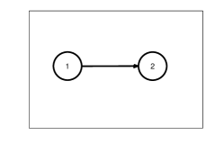
Figure 7: A directed two node graph.

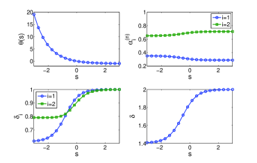
Figure 8: (color online) Simulation results for the directed 2-node graph in fig. 7. See the main text for comments.

References

- Hill and Physics (1987) T. L. Hill and Physics, An Introduction to Statistical Thermodynamics (Dover Books on Physics) (Dover Publications, 1987).
- Sachdev (2011) S. Sachdev, Quantum Phase Transitions, 2nd ed. (Cambridge University Press, 2011).
- Verstraete et al. (2009) F. Verstraete, M. Wolf, and J. Cirac, Nature Physics 5, 633 (2009).
- Diehl et al. (2008) S. Diehl, A. Micheli, A. Kantian, B. Kraus, H. Büchler, and P. Zoller, Nature Physics 4, 878 (2008).
- Kraus et al. (2008) B. Kraus, H. Büchler, S. Diehl, A. Kantian, A. Micheli, and P. Zoller, Physical Review A 78, 042307 (2008).
- Diehl et al. (2010) S. Diehl, A. Tomadin, A. Micheli, R. Fazio, and P. Zoller, Physical review letters 105, 15702 (2010).
- Aharonov et al. (2001) D. Aharonov, A. Ambainis, J. Kempe, and U. Vazirani, in Proceedings of the thirty-third annual ACM symposium on Theory of computing (ACM, 2001) pp. 50–59.
- Farhi and Gutmann (1998) E. Farhi and S. Gutmann, Phys. Rev. A 58, 915 (1998).
- Childs et al. (2002) A. Childs, E. Farhi, and S. Gutmann, Quantum Information Processing 1, 35 (2002).
- Farhi et al. (2008) E. Farhi, J. Goldstone, and S. Gutmann, Theory OF Computing 4, 169 (2008).
- Childs (2009) A. M. Childs, Phys. Rev. Lett. 102, 180501 (2009).
- Mulken and Blumen (2011) O. Mulken and A. Blumen, Physics Reports (2011).
- Tsomokos (2011) D. I. Tsomokos, Phys. Rev. A 83, 052315 (2011).
- Rebentrost et al. (2009a) P. Rebentrost, M. Mohseni, and A. Aspuru-Guzik, The Journal of Physical Chemistry B 113, 9942 (2009a).
- Mohseni et al. (2008) M. Mohseni, P. Rebentrost, S. Lloyd, and A. Aspuru-Guzik, The Journal of Chemical Physics 129, 174106 (2008).
- Plenio and Huelga (2008) M. Plenio and S. Huelga, New Journal of Physics 10, 113019 (2008).
- Caruso et al. (2009) F. Caruso, A. Chin, A. Datta, S. Huelga, and M. Plenio, The Journal of Chemical Physics 131, 105106 (2009).
- Rebentrost et al. (2009b) P. Rebentrost, M. Mohseni, I. Kassal, S. Lloyd, and A. Aspuru-Guzik, New Journal of Physics 11, 033003 (2009b).
- Giorda et al. (2011) P. Giorda, S. Garnerone, P. Zanardi, and S. Lloyd, Arxiv preprint arXiv:1106.1986 (2011).
- Strauch (2009) F. W. Strauch, Phys. Rev. A 79, 032319 (2009).
- Strauch and Williams (2008) F. Strauch and C. Williams, Physical Review B 78, 094516 (2008).
- Whitfield et al. (2010) J. Whitfield, C. Rodríguez-Rosario, and A. Aspuru-Guzik, Physical Review A 81, 022323 (2010).
- Plenio and Knight (1997) M. Plenio and P. Knight, Reviews of Modern Physics 70 (1997).
- Touchette (2009) H. Touchette, Physics Reports 478, 1 (2009).
- Ruelle (2004) D. Ruelle, Thermodynamic formalism: the mathematical structures of equilibrium statistical mechanics (Cambridge Univ Pr, 2004).
- Brin and Page (1998) S. Brin and L. Page, Computer Networks and ISDN Systems 30, 107 (1998).
- Langville and Meyer (2006) A. N. Langville and C. D. Meyer, Google’s PageRank and Beyond: The Science of Search Engine Rankings (Princeton University Press, 2006).
- Shikano (2011) Y. Shikano, in AIP Conference Proceedings, Vol. 1327 (2011) p. 487.
- Venegas-Andraca (2008) S. Venegas-Andraca, Synthesis Lectures on Quantum Computing 1, 1 (2008).
- Breuer and Petruccione (2002) H. Breuer and F. Petruccione, The theory of open quantum systems (Oxford: Oxford University Press, 2002).
- Hedges et al. (2009) L. Hedges, R. Jack, J. Garrahan, and D. Chandler, Science 323, 1309 (2009).
- Garrahan and Lesanovsky (2010) J. Garrahan and I. Lesanovsky, Physical review letters 104, 160601 (2010).
- Garrahan et al. (2007) J. Garrahan, R. Jack, V. Lecomte, E. Pitard, K. van Duijvendijk, and F. van Wijland, Physical review letters 98, 195702 (2007).
- Lebowitz and Spohn (1999) J. Lebowitz and H. Spohn, Journal of Statistical Physics 95, 333 (1999).
- Sánchez-Burillo et al. (2012) E. Sánchez-Burillo, J. Duch, J. Gómez-Gardeñes, and D. Zueco, Scientific Reports 2, 605 (2012).
- Spohn (1977) H. Spohn, Letters in Mathematical Physics 2, 33 (1977).
- Boccaletti et al. (2006) S. Boccaletti, V. Latora, Y. Moreno, M. Chavez, and D. Hwang, Physics reports 424, 175 (2006).
- Barrat et al. (2008) A. Barrat, M. Barthlemy, and A. Vespignani, Dynamical processes on complex networks (Cambridge University Press, 2008).
- Barabási (2002) A.-L. Barabási, Linked: The New Science of Networks, 1st ed. (Basic Books, 2002).
- Barabási (2005) A. Barabási, Nature Physics 1, 68 (2005).
- Giraud et al. (2005) O. Giraud, B. Georgeot, and D. Shepelyansky, Physical Review E 72, 036203 (2005).
- Braunstein et al. (2006) S. Braunstein, S. Ghosh, and S. Severini, Annals of Combinatorics 10, 291 (2006).
- Kimble (2008) H. Kimble, Nature 453, 1023 (2008).
- Lapeyre et al. (2009) G. J. Lapeyre, J. Wehr, and M. Lewenstein, Phys. Rev. A 79, 042324 (2009).
- Perseguers et al. (2010a) S. Perseguers, M. Lewenstein, A. Acín, and J. Cirac, Nature Physics 6, 539 (2010a).
- Perseguers (2010) S. Perseguers, Phys. Rev. A 81, 012310 (2010).
- Perseguers et al. (2010b) S. Perseguers, D. Cavalcanti, G. J. Lapeyre, M. Lewenstein, and A. Acín, Phys. Rev. A 81, 032327 (2010b).
- Anand et al. (2011) K. Anand, G. Bianconi, and S. Severini, Phys. Rev. E 83, 036109 (2011).
- Wu and Zhu (2011) L. Wu and S. Zhu, Phys. Rev. A 84, 052304 (2011).
- Cuquet and Calsamiglia (2011) M. Cuquet and J. Calsamiglia, Phys. Rev. A 83, 032319 (2011).
- Ionicioiu and Spiller (2012) R. Ionicioiu and T. P. Spiller, Phys. Rev. A 85, 062313 (2012).
- Garnerone et al. (2012a) S. Garnerone, P. Zanardi, and D. A. Lidar, Phys. Rev. Lett. 108, 230506 (2012a).
- Paparo and Martin-Delgado (2012) G. D. Paparo and M. A. Martin-Delgado, Scientific Reports 2, 444 (2012).
- Garnerone et al. (2012b) S. Garnerone, P. Giorda, and P. Zanardi, New Journal of Physics 14, 013011 (2012b).
- Adhikari et al. (2012) B. Adhikari, S. Adhikari, and S. Banerjee, Arxiv preprint arXiv:1205.2747 (2012).