Spectroscopic analysis of the two subgiant branches of the globular cluster NGC 1851

It has been found that globular clusters host multiple stellar populations. In particular, in NGC 1851 the subgiant branch (SGB) can be divided into two components and the distribution of stars along the horizontal branch (HB) is multimodal. Various authors have found that NGC 1851 possibly has a spread in [Fe/H], but the relation between this spread and the division in the SGB is unknown. We obtained blue (3950-4600 Å) intermediate resolution ($R\sim 8,000$) spectra for 47 stars on the bright and 30 on the faint SGB of NGC 1851 (b-SGB and f-SGB, respectively). The spectra were analysed by comparing with synthetic spectra. The determination of the atmospheric parameters to extremely high internal accuracy allows small errors to be recovered when comparing different stars in the cluster, in spite of their faintness ($V\sim 19$). Abundances were obtained for Fe, C, Ca, Cr, Sr, and Ba. We found that the b-SGB is slightly more metal-poor than the f-SGB, with [Fe/H]=$-1.227\pm 0.009$ and [Fe/H]=$-1.162\pm 0.012$, respectively. This implies that the f-SGB is only slightly older by $\sim 0.6$ Gyr than the b-SGB if the total CNO abundance is constant. There are more C-normal stars in the b-SGB than in the f-SGB. This is consistent with what is found for HB stars, if b-SGB are the progenitors of red HB stars, and f-SGB those of blue HB ones. As previously found, the abundances of the n-capture elements Sr and Ba have a bimodal distribution, reflecting the separation between f-SGB (Sr and Ba-rich) and b-SGB stars (Sr and Ba-poor). In both groups, there is a clear correlation between [Sr/Fe] and [Ba/Fe], suggesting that there is a real spread in the abundances of n-capture elements. By looking at the distribution of SGB stars in the [C/H] vs. T_eff diagram and in the [Ba/H] vs. [Sr/H] diagram, not a one-to-one relation is found among these quantities. There is some correlation between C and Ba abundances, while the same correlation for Sr is much more dubious. We identified six C-rich stars, which have a moderate overabundance of Sr and Ba and rather low N abundances. This group of stars might be the progenitors of these on the anomalous RGB in the $(v,v-y)$ diagram. These results are discussed within different scenarios for the formation of NGC 1851. It is possible that the two populations originated in different regions of a inhomogeneous parent object. However, the striking similarity with M 22 calls for a similar evolution for these two clusters. Deriving reliable CNO abundances for the two sequences would be crucial.

1 Introduction

Most, possibly all, globular clusters host multiple stellar populations (see reviews in Gratton et al. 2004, 2012a). The most sensitive diagnostics of these populations is the Na-O anticorrelation (Kraft 1994; Gratton et al. 2004), although very important information is also provided by the colour-magnitude diagram (see Piotto 2009; Gratton et al. 2010). In the majority of cases, available observations can be explained by two generations of stars: a primordial population, with the same chemical composition as field halo stars of similar metallicity; and a second generation, born from the ejecta of a fraction of the stars of the earlier one. The nature of the first generation of stars whose ejecta are used to form the second generation is still debated: they may be massive AGB stars undergoing hot bottom burning (see e.g. Ventura et al. 2001) or rapidly rotating massive stars (see e.g. Decressin et al. 2007; etc.). In addition, it is clear that the whole process is driven mainly by the total mass of the cluster (Carretta et al. 2010a), even though other parameters might have a role (location in the galaxy, orbit, etc.). However, there are a few cases that do not easily fit in this scenario and possibly require additional mechanisms to create multiple stellar populations. One of these anomalies is related to the splitting of the subgiant branch (SGB) which is observed in a few clusters, the most notable cases being NGC 1851 (Milone et al. 2008, 2009; Han et al. 2009) and M22 (=NGC 6656: Piotto 2009). This splitting might be attributed to either a quite large difference in age (of the order of 1 Gyr: Milone et al. 2008) or CNO content (by at least a factor of two: Cassisi et al. 2008). Both of these features cannot be easily related to the usual second generation scenario, where the age difference between the first/primordial and the second generation is thought to be less than 100 Myr, and no significant alteration of the sum of CNO elements is foreseen (see Carretta et al. 2005; Villanova et al. 2010, Yong et al. 2011). This calls for additional mechanisms that are not yet understood.

Both NGC 1851 and M22 have been studied quite extensively in the past few years. High dispersion spectra have been obtained for red giants (Yong & Grundahl 2008; Villanova et al. 2010; Carretta et al. 2010c, 2011a; Marino et al. 2011; Roederer et al. 2011) and horizontal branch (HB) stars (Gratton et al. 2012b). Marino et al. (2012) and Lardo et al. (2012) also obtained intermediate and low resolution spectra of SGB stars in M22 and NGC 1851, respectively. In addition, Strömgren photometry was obtained for red giant branch (RGB) stars by Grundahl et al. (1999) and Lee et al. (2009), and recently discussed by Carretta et al. (2011a, 2011b) and Lardo et al. (2012). This quite impressive dataset showed that the two clusters (which differ in metallicity by some 0.5 dex) appear to share numerous observational features. In both cases, there is evidence of a spread in metal abundance that is larger in M22 ($\sim 0.2$ dex in [Fe/H]) but also present in NGC 1851 (Lee et al 2009; Carretta et al. 2010b, 2010c, 2011a), although Villanova et al. (2010) found no evidence of an Fe spread among RGB stars from the split RGB. The neutron-capture elements that are mainly produced by the $s$-process are also found to have widely different star-to-star abundances that are correlated with both [Fe/H] and the abundances of light, proton-capture elements (Carretta et al. 2011a). Finally, a spread in the abundances of individual CNO elements has been found within both the bright and faint SGB (b-SGB and f-SGB, respectively), that is also correlated with the variation in heavier elements (Marino et al. 2012; Lardo et al. 2012).

NGC 1851 has additional peculiarities that have not yet been found in M22 where no bimodality in the HB exists, at least in the CMD, exists. The most obvious peculiarity is the bimodal distribution of stars along the HB (Walker 1992): about 60% of the stars reside on the red horizontal branch (RHB), some 30% being on the blue horizontal branch (BHB), and only 10% of the stars having intermediate colours that fall within the instability strip. It is unclear whether the difference in the distribution of stars along the HB with respect to M22 - where no bimodality has yet been discovered - might be explained simply by the different metallicity and age of the two clusters, or to some more significant difference in their formation scenarios. Gratton et al. (2012b) studied the chemical composition of about a hundred HB stars in NGC 1851. They found that both red and blue HB stars display separate Na-O anticorrelations, reinforcing the suggestion advanced by van den Bergh (1996), Catelan (1997), Carretta et al. (2010c, 2011a), and Bekki and Yong (2012) that NGC 1851 might possibly be the result of the merging of two clusters (another cluster which may be interesting in this context is Terzan 5, which also has a bimodal HB: see Ferraro et al. 2009 and Origlia et al. 2011). However, other observational results remain unexplained. There is a group of RHB stars with high Ba (and Na) abundances. These stars might possibly be related to the anomalous red sequence in the Strömgren $(v,v-y)$ diagram considered by Villanova et al. (2010) and Carretta et al. (2011a), which also exclusively consists of Ba-rich stars (Villanova et al. 2010), although Carretta et al. (2011a) found many other Ba-rich red giants in NGC 1851. A possible way of explaining the anomalous position of these stars in the $(v,v-y)$ diagram is to assume that they have a larger CNO content (see Carretta et al. 2011c and Gratton et al. 2012b). The sum of the abundances of CNO elements of these stars in NGC 1851 is debated: Yong & Grundahl (2008) and Yong et al. (2011; see Alves-Brito et al., 2012, for a similar claim for M 22) found indications of a large enhancement, while Villanova et al. (2010) instead found that they have a constant, low/normal CNO content. In all cases, this sequence contains $\sim 10-15$% of the stars, and can thus correspond directly to neither the f-SGB sequence (which consists of some 30-40% of the SGB stars of NGC 1851: Milone et al. 2008, 2009) nor the BHB (which makes up a similar fraction of the HB stars: Milone et al. 2009).

On the other hand, Han et al. (2009) found that the progeny of the f-SGB can be followed throughout the RGB in the $(U,U-I)$ diagram. A very similar result was obtained by Lardo et al. (2012) by using a particular combination of Strömgren colours ($(u+v)-(b+y)$). This combination, which compares the sum of the ultraviolet (UV) and violet magnitudes with sum of the blue and yellow ones, is actually conceptually similar to the Han et al. broad band photometry. In both cases, the clear separation of stars in these sequences might be caused by a combination of different effective temperatures and absorption by atomic lines and molecular bands in the UV, so that its interpretation in terms of abundances is not simple: Han et al. attributed the difference to heavy elements, Lardo et al. to CNO, and Carretta et al. (2010b, 2011b) found that it is very well-correlated with O and Na abundances on the upper part of the RGB. Lardo et al. found that summing up these stars over the whole RGB, the fraction is $\sim 30$%, as for f-SGB stars. Stars on the anomalous RGB in the $(v,v-y)$ diagram are however only a subset of the ”red” stars in the $(U,U-I)$ or $(u,(u-y)+(v-b))$ diagrams, and should result from the evolution of only part of the f-SGB stars.

A detailed study of the chemical composition of stars on both the bright (b-SGB) and faint (f-SGB) sequences of NGC 1851 might help us to understand the evolutionary history of this cluster, providing constraints on the ages and chemical compositions of its various populations. The SGB is possibly the part of the colour-magnitude diagram where subtle age differences may best be proven, but at present we do not even know the metallicity ranking of the two most important populations present in this cluster. Metallicity is a basic ingredient in age derivations, and even small abundance differences may have an impact in a case such as NGC 1851. Unfortunately, SGB stars are quite faint in such a distant cluster, so that high resolution spectra would require a prohibitively long exposure time even on eight meter class telescopes. Lardo et al. (2012) presented an analysis of low-resolution spectra for a total of 64 stars near the SGB of NGC 1851: they found separate C-N anticorrelations for stars on the two branches, and evidence that on average the sums of C+N differ by a factor of 2.5 between them. However, the spectra they used have a low resolution ($R\sim 1,000$) and they adopted a temperature scale that is apparently inconsistent with the evolutionary status of the stars observed. These facts cast doubts on their conclusions.

In this paper, we present the results of the analysis of new intermediate-resolution ($R\sim 8,000$) blue spectra of about eighty stars on the SGB of NGC 1851. These intermediate resolution spectra do not allow us to derive the abundances from weak lines, hence we are limited in the available diagnostics. However, we show that very useful information can be gathered once adequate care is taken in critical aspects of the analysis. The structure of this paper is as follows: the observational material is presented in Section 2; the analysis methods - which are quite unusual and were specially tailored for our case - are described in Section 3; our results are presented in Section 4. Discussion and conclusions are drawn in Section 5.

Figure 1: Top: Advanced Camera for Surveys colour-magnitude diagram for the subgiant branch of NGC 1851 from Milone et al. (2008). Bottom: The same, but using ground-based data. Observed stars on the b-SGB (filled circles) and f-SGB (open circles) are shown.

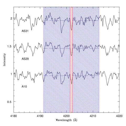
Figure 2: Portion of the spectra of three SGB stars of NGC 1851, including the strong Fe line at 4202 Å (AS31, AS29, and A10). Spectra of the first two stars have been shifted vertically for clarity. This is one of the fifteen strong Fe lines used in our Fe abundance derivation. The areas hatched in red and blue mark the regions used to evaluate the line index appropriate for this line as described in the text (red is the in-line region, blue is the reference one). The average flux within each of these regions are shown as horizontal dashed lines.

2 Observations and data reduction

Target stars on both the two SGBs were selected from the Advanced Camera for Survey (ACS) of the Hubble Space Telescope (HST) (Milone et al. 2008) and ground-based $VI$ photometry performed by Stetson, as described in Milone et al. (2009). In the first case, the high-precision photometry allowed a straightforward assignment of each star to its respective SGB, in the second some degree of uncertainty is present because the two SGBs are not so clearly separated, especially in the reddest part ($V-I>1.3$). Observed objects are shown in Fig. 1 as filled circles (b-SGB) and open circles (f-SGB), respectively.

The spectra were acquired with the GIRAFFE fibre-fed spectrograph at the Very Large Telescope (VLT) (Pasquini et al. 2004) under the ESO programme 084.D-0470 (PI Villanova), using the LR02 grating. They cover approximately the wavelength range 3950-4560 Å at a resolution of about 0.5 Å (FWHM). In this spectral range, there are many strong lines of H, Fe, Ca, Sr, Ba, and CH, as well as many other lines that were not used in the present analysis. Targets are quite faint (V$\sim$19), so for each we obtained 20$\times$45 min spectra in order to reach the required signal-to-noise (S/N) ($\sim$50). The spectra were reduced by the ESO personnel using the ESO FLAMES GIRAFFE pipeline version 2.8.7, and then rectified to an approximate continuum value. This was done in a homogeneous way for all spectra, and turned out to be very useful for our analysis. However, we should take into account the possibility that some systematic difference is induced by this rectification depending on for instance S/N of the spectra or temperature of the stars. In all cases, this ”rectification” of the spectra does not have the same meaning as tracing a continuum in high dispersion spectra, because at the resolution of the spectra no pixels remain unaffected by absorption of some spectral lines. This was considered in our analysis.

We measured radial velocities using the fxcor package in IRAF, adopting a synthetic spectrum as a template. All stars turned out to have a velocity compatible with that of the cluster confirming their membership. We obtained an average radial velocity of $318.2\pm 0.5$ km s^-1  with a root mean square (r.m.s.) scatter of 4.3 km s^-1; very similar results were obtained by considering separately b-SGB and f-SGB stars. For comparison, Scarpa et al. (2011) found an average velocity of $320.0\pm 0.4$ km s^-1 with an r.m.s. of 4.9 km s^-1 for 184 SGB stars, and that the cluster is slowly rotating (see also Bellazzini et al. 2012). Similar values were obtained by Carretta et al. (2011b) for stars on the RGB ($320.3\pm 0.4$ km s^-1, r.m.s. of 3.7 km s^-1), and by Gratton et al. (2012b) for stars on the RHB ($319.7\pm 0.5$ km s^-1, r.m.s. of 3.7 km s^-1), BHB ($321.6\pm 0.7$ km s^-1, r.m.s. of 4.1 km s^-1), and lower RGB ($320.3\pm 1.0$ km s^-1, r.m.s. of 3.6 km s^-1). The offsets between these different sets of radial velocity data are nominally larger than the statistical errors. In principle, we might expect to find small offsets between the average radial velocities for stars in different evolutionary phases that are produced by convective motions and gravitational redshifts; however, in the present study they are most likely due to systematic differences among results obtained using different gratings and templates. Before any additional step could be made, the spectra were then reduced to zero radial velocity.

A small portion of each of the spectra of three stars is shown in Figure 2.

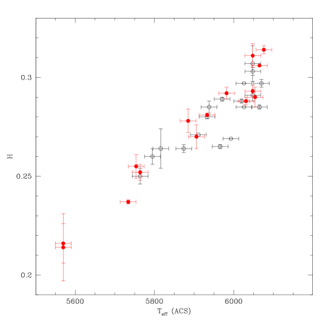
Figure 3: Comparison of temperatures derived using the ACS F606W-F814W colour and the parameter H describing the strengths of H$\gamma$ and H$\delta$. Filled red symbols are for f-SGB stars, and empty black symbols represent b-SGB ones.

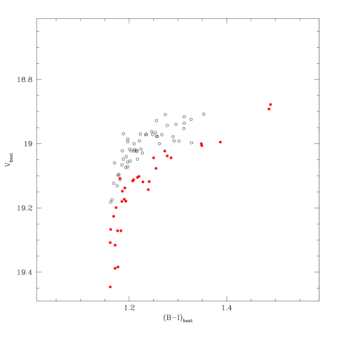
Figure 4: Pseudo colour-magnitude diagram obtained using our pseudo-colour $(B-I)_{\rm best}$. Symbols are as in Figure 3.

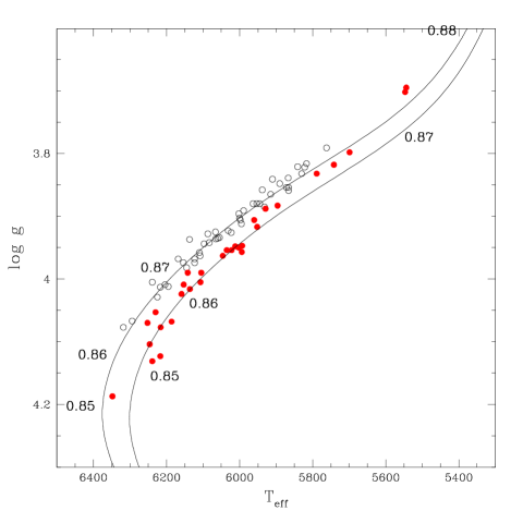
Figure 5: Distribution of the programme stars in the effective temperature-surface gravity plane. Symbols are as in Figure 3. We overimpose two $\alpha$-enhanced isochrones from the BASTI database (Pietrinferni et al. 2006), which were computed for [Fe/H] values appropriate to the two sequences ([Fe/H]=-1.22 and -1.17) and ages of 10.1 and 10.7 Gyr for b-SGB and f-SGB, respectively. Stellar masses along these isochrones are also given.

3 Analysis

Table 1: Atmospheric parameters and abundances in the program stars - Bright SGB

ID	$T_{\rm eff}$	$\log{g}$	$v_{t}$	$[$Fe/H$]$	$[$C/Fe$]$	$[$Ca/Fe$]$	$[$Cr/Fe$]$	$[$Sr/Fe$]$	$[$Ba/Fe$]$	$\Delta u-y$
	(K)		(km s-1)
A10	$6002\pm 21$	3.895	0.97	$-1.23\pm 0.04$	$-0.08\pm 0.03$	0.30	-0.36	$\leavevmode\nobreak\ \leavevmode\nobreak\ 0.14\pm 0.10$	0.81	-0.016
A12	$5989\pm 21$	3.890	0.97	$-1.22\pm 0.04$	$\leavevmode\nobreak\ \leavevmode\nobreak\ 0.11\pm 0.01$	0.49	-0.16	$-0.10\pm 0.20$	1.02	0.108
A13	$5915\pm 21$	3.864	0.98	$-1.42\pm 0.03$	$\leavevmode\nobreak\ \leavevmode\nobreak\ 0.25\pm 0.01$	0.43	0.02	$\leavevmode\nobreak\ \leavevmode\nobreak\ 0.15\pm 0.06$	0.95	0.054
A16	$5953\pm 21$	3.879	0.97	$-1.20\pm 0.03$	$-0.12\pm 0.02$	0.41	-0.36	$\leavevmode\nobreak\ \leavevmode\nobreak\ 0.27\pm 0.05$	1.10	0.325
A17	$6000\pm 21$	3.902	0.96	$-1.13\pm 0.03$	$-0.03\pm 0.02$	0.31	-0.02	$-0.09\pm 0.17$	0.56	0.133
A21	$5762\pm 21$	3.790	1.00	$-1.14\pm 0.03$	$\leavevmode\nobreak\ \leavevmode\nobreak\ 0.01\pm 0.03$	0.45	-0.04	$\leavevmode\nobreak\ \leavevmode\nobreak\ 0.11\pm 0.02$	0.88	0.001
A23	$6087\pm 21$	3.927	0.96	$-1.26\pm 0.04$	$\leavevmode\nobreak\ \leavevmode\nobreak\ 0.26\pm 0.02$	0.31	-0.10	$-0.01\pm 0.10$	0.94	0.062
A24	$5817\pm 21$	3.815	0.99	$-1.18\pm 0.03$	$\leavevmode\nobreak\ \leavevmode\nobreak\ 0.08\pm 0.03$	0.36	-0.41	$\leavevmode\nobreak\ \leavevmode\nobreak\ 0.01\pm 0.06$	0.69	-0.015
A25	$5945\pm 21$	3.879	0.97	$-1.22\pm 0.02$	$-0.01\pm 0.02$	0.32	-0.18	$\leavevmode\nobreak\ \leavevmode\nobreak\ 0.23\pm 0.00$	1.04	0.002
A27	$5872\pm 21$	3.853	0.98	$-1.11\pm 0.03$	$-0.05\pm 0.02$	0.27	-0.11	$\leavevmode\nobreak\ \leavevmode\nobreak\ 0.18\pm 0.03$	0.58	0.004
A29	$5998\pm 21$	3.905	0.96	$-1.26\pm 0.04$	$\leavevmode\nobreak\ \leavevmode\nobreak\ 0.10\pm 0.02$	0.37	-0.22	$-0.03\pm 0.13$	0.83	0.099
A30	$5995\pm 21$	3.911	0.96	$-1.20\pm 0.03$	$\leavevmode\nobreak\ \leavevmode\nobreak\ 0.08\pm 0.02$	0.37	-0.08	$\leavevmode\nobreak\ \leavevmode\nobreak\ 0.18\pm 0.07$	0.74	0.083
A34	$5867\pm 21$	3.838	0.98	$-1.20\pm 0.03$	$\leavevmode\nobreak\ \leavevmode\nobreak\ 0.09\pm 0.04$	0.42	-0.24	$\leavevmode\nobreak\ \leavevmode\nobreak\ 0.14\pm 0.03$	0.52	0.057
A35	$6060\pm 21$	3.934	0.95	$-1.25\pm 0.03$	$-0.05\pm 0.01$	0.34	-0.03	$\leavevmode\nobreak\ \leavevmode\nobreak\ 0.17\pm 0.17$	0.93	0.108
A03	$5841\pm 21$	3.820	0.99	$-1.16\pm 0.03$	$-0.13\pm 0.01$	0.44	-0.26	$\leavevmode\nobreak\ \leavevmode\nobreak\ 0.16\pm 0.03$	0.83	-0.034
A04	$6110\pm 21$	3.957	0.95	$-1.21\pm 0.05$	$-0.15\pm 0.05$	0.34	-0.10	$\leavevmode\nobreak\ \leavevmode\nobreak\ 0.21\pm 0.01$	0.99	0.120
A06	$5910\pm 21$	3.840	0.98	$-1.31\pm 0.04$	$\leavevmode\nobreak\ \leavevmode\nobreak\ 0.14\pm 0.02$	0.37	-0.31	$-0.04\pm 0.09$	0.89	-0.039
A09	$6066\pm 21$	3.924	0.96	$-1.30\pm 0.03$	$\leavevmode\nobreak\ \leavevmode\nobreak\ 0.23\pm 0.00$	0.38	-0.19	$\leavevmode\nobreak\ \leavevmode\nobreak\ 0.28\pm 0.07$	0.86	-0.040
AS12	$5830\pm 23$	3.831	0.99	$-1.27\pm 0.03$	$-0.19\pm 0.00$	0.37	-0.32	$\leavevmode\nobreak\ \leavevmode\nobreak\ 0.02\pm 0.12$	0.70	-0.055
AS14	$5866\pm 23$	3.858	0.98	$-1.21\pm 0.03$	$\leavevmode\nobreak\ \leavevmode\nobreak\ 0.11\pm 0.03$	0.38	-0.38	$\leavevmode\nobreak\ \leavevmode\nobreak\ 0.08\pm 0.10$	0.93	-0.017
AS15	$6097\pm 23$	3.943	0.95	$-1.15\pm 0.03$	$\leavevmode\nobreak\ \leavevmode\nobreak\ 0.17\pm 0.03$	0.31	0.14	$\leavevmode\nobreak\ \leavevmode\nobreak\ 0.28\pm 0.02$	1.03
AS18	$6031\pm 23$	3.922	0.96	$-1.24\pm 0.03$	$-0.16\pm 0.04$	0.39	-0.29	$\leavevmode\nobreak\ \leavevmode\nobreak\ 0.17\pm 0.01$	0.81	0.040
AS22	$6002\pm 23$	3.895	0.97	$-1.25\pm 0.03$	$\leavevmode\nobreak\ \leavevmode\nobreak\ 0.22\pm 0.02$	0.42	0.05	$\leavevmode\nobreak\ \leavevmode\nobreak\ 0.19\pm 0.09$	0.88
AS24	$5866\pm 23$	3.853	0.98	$-1.21\pm 0.04$	$-0.01\pm 0.00$	0.46	-0.07	$\leavevmode\nobreak\ \leavevmode\nobreak\ 0.06\pm 0.03$	1.04	-0.012
AS25	$5945\pm 23$	3.879	0.97	$-1.21\pm 0.04$	$\leavevmode\nobreak\ \leavevmode\nobreak\ 0.09\pm 0.03$	0.44	-0.14	$\leavevmode\nobreak\ \leavevmode\nobreak\ 0.15\pm 0.08$	0.93	-0.151
AS28	$6168\pm 23$	3.967	0.94	$-1.30\pm 0.04$	$\leavevmode\nobreak\ \leavevmode\nobreak\ 0.37\pm 0.01$	0.58	0.35	$\leavevmode\nobreak\ \leavevmode\nobreak\ 0.32\pm 0.16$	0.83	0.037
AS29	$6204\pm 23$	4.008	0.93	$-1.32\pm 0.05$	$\leavevmode\nobreak\ \leavevmode\nobreak\ 0.31\pm 0.03$	0.43	0.21	$\leavevmode\nobreak\ \leavevmode\nobreak\ 0.52\pm 0.04$	1.01	0.031
AS02	$6318\pm 23$	4.076	0.91	$-1.11\pm 0.04$	$\leavevmode\nobreak\ \leavevmode\nobreak\ 0.07\pm 0.06$	0.21	-0.02	$-0.02\pm 0.23$	0.81
AS31	$5822\pm 23$	3.821	0.99	$-1.21\pm 0.04$	$\leavevmode\nobreak\ \leavevmode\nobreak\ 0.14\pm 0.03$	0.37	-0.19	$\leavevmode\nobreak\ \leavevmode\nobreak\ 0.07\pm 0.06$	0.80
AS36	$6217\pm 23$	4.012	0.93	$-1.33\pm 0.06$	$\leavevmode\nobreak\ \leavevmode\nobreak\ 0.33\pm 0.05$	0.59	0.51	$\leavevmode\nobreak\ \leavevmode\nobreak\ 0.50\pm 0.08$	1.20
AS37	$6065\pm 23$	3.935	0.95	$-1.17\pm 0.03$	$-0.04\pm 0.03$	0.30	-0.33	$\leavevmode\nobreak\ \leavevmode\nobreak\ 0.14\pm 0.03$	0.85	-0.016
AS38	$5938\pm 23$	3.857	0.98	$-1.22\pm 0.03$	$\leavevmode\nobreak\ \leavevmode\nobreak\ 0.14\pm 0.01$	0.24	-0.02	$\leavevmode\nobreak\ \leavevmode\nobreak\ 0.12\pm 0.09$	0.82
AS39	$5932\pm 23$	3.884	0.97	$-1.30\pm 0.04$	$\leavevmode\nobreak\ \leavevmode\nobreak\ 0.23\pm 0.03$	0.48	-0.25	$\leavevmode\nobreak\ \leavevmode\nobreak\ 0.47\pm 0.02$	1.03	-0.072
AS40	$6294\pm 23$	4.066	0.91	$-1.18\pm 0.05$	$\leavevmode\nobreak\ \leavevmode\nobreak\ 0.21\pm 0.02$	0.60	0.24	$\leavevmode\nobreak\ \leavevmode\nobreak\ 0.42\pm 0.07$	1.19	0.004
AS42	$6108\pm 23$	3.962	0.94	$-1.30\pm 0.06$	$\leavevmode\nobreak\ \leavevmode\nobreak\ 0.31\pm 0.04$	0.27	0.24	$\leavevmode\nobreak\ \leavevmode\nobreak\ 0.34\pm 0.05$	1.26	-0.013
AS43	$6225\pm 23$	4.028	0.92	$-1.24\pm 0.04$	$\leavevmode\nobreak\ \leavevmode\nobreak\ 0.32\pm 0.03$	0.52	-0.16	$\leavevmode\nobreak\ \leavevmode\nobreak\ 0.04\pm 0.00$	0.83	0.055
AS44	$5890\pm 23$	3.847	0.98	$-1.23\pm 0.03$	$\leavevmode\nobreak\ \leavevmode\nobreak\ 0.03\pm 0.02$	0.47	-0.14	$\leavevmode\nobreak\ \leavevmode\nobreak\ 0.23\pm 0.02$	0.92	-0.028
AS45	$6154\pm 23$	3.973	0.94	$-1.17\pm 0.05$	$\leavevmode\nobreak\ \leavevmode\nobreak\ 0.21\pm 0.00$	0.41	0.10	$\leavevmode\nobreak\ \leavevmode\nobreak\ 0.11\pm 0.08$	0.84	-0.048
AS46	$6195\pm 23$	4.011	0.93	$-1.19\pm 0.05$	$\leavevmode\nobreak\ \leavevmode\nobreak\ 0.25\pm 0.01$	0.33	-0.19	$\leavevmode\nobreak\ \leavevmode\nobreak\ 0.03\pm 0.06$	0.79	-0.007
AS48	$6145\pm 23$	3.981	0.94	$-1.22\pm 0.04$	$\leavevmode\nobreak\ \leavevmode\nobreak\ 0.21\pm 0.03$	0.31	-0.19	$\leavevmode\nobreak\ \leavevmode\nobreak\ 0.11\pm 0.02$	0.79	-0.045
AS04	$6123\pm 23$	3.973	0.94	$-1.25\pm 0.05$	$\leavevmode\nobreak\ \leavevmode\nobreak\ 0.15\pm 0.03$	0.33	-0.12	$\leavevmode\nobreak\ \leavevmode\nobreak\ 0.35\pm 0.11$	1.07	-0.015
AS50	$6239\pm 23$	4.004	0.93	$-1.20\pm 0.05$	$\leavevmode\nobreak\ \leavevmode\nobreak\ 0.31\pm 0.02$	0.61	-0.21	$\leavevmode\nobreak\ \leavevmode\nobreak\ 0.12\pm 0.07$	1.09
AS54	$6083\pm 23$	3.941	0.95	$-1.16\pm 0.04$	$\leavevmode\nobreak\ \leavevmode\nobreak\ 0.26\pm 0.02$	0.46	0.09	$\leavevmode\nobreak\ \leavevmode\nobreak\ 0.46\pm 0.05$	1.09
AS56	$6123\pm 23$	3.967	0.94	$-1.28\pm 0.04$	$\leavevmode\nobreak\ \leavevmode\nobreak\ 0.06\pm 0.08$	0.43	0.12	$\leavevmode\nobreak\ \leavevmode\nobreak\ 0.34\pm 0.03$	0.70
AS05	$6023\pm 23$	3.925	0.96	$-1.26\pm 0.06$	$-0.09\pm 0.04$	0.35	-0.05	$\leavevmode\nobreak\ \leavevmode\nobreak\ 0.16\pm 0.12$	0.66
AS08	$6055\pm 23$	3.933	0.95	$-1.20\pm 0.04$	$-0.17\pm 0.09$	0.23	0.08	$\leavevmode\nobreak\ \leavevmode\nobreak\ 0.12\pm 0.03$	0.47
AS09	$5963\pm 23$	3.879	0.97	$-1.27\pm 0.04$	$\leavevmode\nobreak\ \leavevmode\nobreak\ 0.23\pm 0.03$	0.37	-0.28	$\leavevmode\nobreak\ \leavevmode\nobreak\ 0.17\pm 0.04$	0.77

Table 2: Atmospheric parameters and abundances in the program stars - Faint SGB

ID	$T_{\rm eff}$	$\log{g}$	$v_{t}$	$[$Fe/H$]$	$[$C/Fe$]$	$[$Ca/Fe$]$	$[$Cr/Fe$]$	$[$Sr/Fe$]$	$[$Ba/Fe$]$	$\Delta u-y$
	(K)		(km s-1)
B10	$5952\pm 21$	3.916	0.96	$-1.24\pm 0.04$	$\leavevmode\nobreak\ \leavevmode\nobreak\ 0.02\pm 0.05$	0.40	0.06	$\leavevmode\nobreak\ \leavevmode\nobreak\ 0.41\pm 0.03$	0.93	0.098
B11	$6022\pm 21$	3.953	0.95	$-1.23\pm 0.03$	$\leavevmode\nobreak\ \leavevmode\nobreak\ 0.05\pm 0.02$	0.50	-0.02	$\leavevmode\nobreak\ \leavevmode\nobreak\ 0.40\pm 0.02$	1.03	0.066
B12	$6046\pm 21$	3.962	0.94	$-1.19\pm 0.03$	$\leavevmode\nobreak\ \leavevmode\nobreak\ 0.20\pm 0.02$	0.43	0.05	$\leavevmode\nobreak\ \leavevmode\nobreak\ 0.37\pm 0.03$	1.20	-0.048
B13	$5547\pm 21$	3.701	1.03	$-1.04\pm 0.03$	$-0.37\pm 0.03$	0.40	-0.06			0.329
B15	$6107\pm 21$	4.004	0.93	$-1.13\pm 0.04$	$-0.19\pm 0.06$	0.35	-0.02	$\leavevmode\nobreak\ \leavevmode\nobreak\ 0.38\pm 0.01$	0.85	0.288
B16	$6002\pm 21$	3.949	0.95	$-1.13\pm 0.03$	$-0.20\pm 0.05$	0.43	-0.17	$\leavevmode\nobreak\ \leavevmode\nobreak\ 0.40\pm 0.17$	0.93	0.108
B18	$5789\pm 21$	3.831	0.99	$-1.15\pm 0.04$	$\leavevmode\nobreak\ \leavevmode\nobreak\ 0.00\pm 0.04$	0.48	-0.03	$\leavevmode\nobreak\ \leavevmode\nobreak\ 0.33\pm 0.10$	1.06	0.044
B01	$5544\pm 21$	3.694	1.03	$-1.12\pm 0.03$	$-0.34\pm 0.04$	0.59	-0.23			-0.004
B02	$6142\pm 21$	3.989	0.94	$-1.25\pm 0.03$	$\leavevmode\nobreak\ 0.03\pm 0.04$	0.25	-0.07	$\leavevmode\nobreak\ \leavevmode\nobreak\ 0.17\pm 0.11$	1.04	0.105
B03	$5929\pm 21$	3.887	0.97	$-1.10\pm 0.03$	$-0.15\pm 0.03$	0.40	-0.05	$\leavevmode\nobreak\ \leavevmode\nobreak\ 0.33\pm 0.01$	1.04	0.126
B04	$5742\pm 21$	3.817	0.99	$-1.13\pm 0.03$	$-0.24\pm 0.02$	0.36	-0.15	$\leavevmode\nobreak\ \leavevmode\nobreak\ 0.30\pm 0.03$	1.11	0.343
B05	$6012\pm 21$	3.947	0.95	$-1.22\pm 0.03$	$-0.11\pm 0.02$	0.44	-0.18	$\leavevmode\nobreak\ \leavevmode\nobreak\ 0.45\pm 0.00$	1.11	0.102
B06	$6105\pm 21$	3.989	0.94	$-1.09\pm 0.03$	$-0.11\pm 0.02$	0.34	0.01	$\leavevmode\nobreak\ \leavevmode\nobreak\ 0.31\pm 0.01$	1.02	0.168
B07	$5896\pm 21$	3.882	0.97	$-1.20\pm 0.04$	$-0.01\pm 0.02$	0.40	-0.18	$\leavevmode\nobreak\ \leavevmode\nobreak\ 0.42\pm 0.05$	1.12	0.139
B09	$5699\pm 21$	3.797	1.00	$-1.22\pm 0.03$	$-0.14\pm 0.00$	0.39	-0.41	$\leavevmode\nobreak\ \leavevmode\nobreak\ 0.37\pm 0.24$	1.15	0.069
BS10	$6186\pm 23$	4.067	0.91	$-1.12\pm 0.05$	$\leavevmode\nobreak\ \leavevmode\nobreak\ 0.16\pm 0.03$	0.17	-0.09	$\leavevmode\nobreak\ \leavevmode\nobreak\ 0.21\pm 0.00$	0.57	-0.003
BS11	$6136\pm 23$	4.015	0.93	$-1.19\pm 0.04$	$-0.03\pm 0.05$	0.37	-0.05	$\leavevmode\nobreak\ \leavevmode\nobreak\ 0.37\pm 0.05$	1.11	0.003
BS12	$6230\pm 23$	4.052	0.92	$-1.08\pm 0.05$	$\leavevmode\nobreak\ \leavevmode\nobreak\ 0.23\pm 0.01$	0.40	0.03	$\leavevmode\nobreak\ \leavevmode\nobreak\ 0.26\pm 0.08$	1.16
BS14	$6246\pm 23$	4.103	0.90	$-1.16\pm 0.03$	$\leavevmode\nobreak\ \leavevmode\nobreak\ 0.03\pm 0.03$	0.49	0.10	$\leavevmode\nobreak\ \leavevmode\nobreak\ 0.46\pm 0.03$	1.26	0.060
BS16	$5960\pm 23$	3.905	0.96	$-1.22\pm 0.05$	$\leavevmode\nobreak\ \leavevmode\nobreak\ 0.44\pm 0.03$	0.37	0.07	$\leavevmode\nobreak\ \leavevmode\nobreak\ 0.43\pm 0.01$	1.27	0.128
BS17	$6159\pm 23$	4.023	0.92	$-1.22\pm 0.04$	$\leavevmode\nobreak\ \leavevmode\nobreak\ 0.15\pm 0.06$	0.43	0.04	$\leavevmode\nobreak\ \leavevmode\nobreak\ 0.53\pm 0.00$	1.28	0.185
BS18	$6153\pm 23$	4.008	0.93	$-1.13\pm 0.04$	$\leavevmode\nobreak\ \leavevmode\nobreak\ 0.07\pm 0.01$	0.46	0.13	$\leavevmode\nobreak\ \leavevmode\nobreak\ 0.24\pm 0.52$	1.09
BS19	$6348\pm 23$	4.186	0.87	$-1.13\pm 0.05$	$\leavevmode\nobreak\ \leavevmode\nobreak\ 0.36\pm 0.04$	0.56	0.40	$\leavevmode\nobreak\ \leavevmode\nobreak\ 0.48\pm 0.04$	1.35
BS20	$6252\pm 23$	4.069	0.91	$-1.13\pm 0.05$	$\leavevmode\nobreak\ \leavevmode\nobreak\ 0.22\pm 0.07$	0.54	0.19	$\leavevmode\nobreak\ \leavevmode\nobreak\ 0.47\pm 0.00$	1.25
BS21	$5993\pm 23$	3.946	0.95	$-1.21\pm 0.03$	$-0.18\pm 0.06$	0.39	-0.07	$\leavevmode\nobreak\ \leavevmode\nobreak\ 0.37\pm 0.04$	1.16
BS03	$6217\pm 23$	4.122	0.89	$-1.27\pm 0.03$	$\leavevmode\nobreak\ \leavevmode\nobreak\ 0.14\pm 0.02$	0.41	0.05	$\leavevmode\nobreak\ \leavevmode\nobreak\ 0.33\pm 0.05$	1.11	0.021
BS04	$6216\pm 23$	4.076	0.91	$-1.22\pm 0.07$	$\leavevmode\nobreak\ \leavevmode\nobreak\ 0.12\pm 0.03$	0.46	-0.36	$\leavevmode\nobreak\ \leavevmode\nobreak\ 0.45\pm 0.05$	1.30
BS06	$6035\pm 23$	3.953	0.95	$-1.05\pm 0.03$	$-0.19\pm 0.05$	0.36	0.10	$\leavevmode\nobreak\ \leavevmode\nobreak\ 0.32\pm 0.15$	0.60	0.068
BS08	$5994\pm 23$	3.956	0.95	$-1.29\pm 0.05$	$\leavevmode\nobreak\ \leavevmode\nobreak\ 0.39\pm 0.04$	0.34	0.12	$\leavevmode\nobreak\ \leavevmode\nobreak\ 0.55\pm 0.29$	1.13	0.013
BS09	$6239\pm 23$	4.130	0.89	$-1.00\pm 0.05$	$\leavevmode\nobreak\ \leavevmode\nobreak\ 0.16\pm 0.07$	0.26	-0.31	$\leavevmode\nobreak\ \leavevmode\nobreak\ 0.00\pm 0.36$	0.90	0.022

3.1 Determination of the atmospheric parameters

The main purpose of our analysis was to study the internal spread in the abundances within NGC 1851 and to look for systematic differences between the b- and f-SGB stars. We emphasize that we made no attempt to derive accurate absolute values for the average abundances within the cluster. Our goal requires the determination of atmospheric parameters with small errors when comparing different stars in similar evolutionary phases, while systematic errors affecting all programme stars in a similar way are less of a concern. However, we found that in spite of the large uncertainties in the abundances derived from blue spectra of intermediate resolution, the average abundances we obtained agree well with those found for stars in other evolutionary phases in this cluster and allow a consistent fit to the colour-magnitude diagram (CMD). We are aware that this might be the result of our compensation for the errors, but we still deem this as a satisfactory result.

The first step in our analysis was the derivation of effective temperatures; for practical reasons, they were ultimately based on the scale used in the BASTI isochrones (Pietrinferni et al. 2006). We used a reddening of E(B-V)=0.02 as listed by Harris (1996) and a preliminary metallicity of [Fe/H]=-1.10, which is slightly higher than the final derived value but this small difference only affects the absolute, not relative values). Very accurate photometry in the F606W and F814W bands from ACS at HST is available from Milone et al. (2008, 2009). This photometry, however, only covers the central portion of the cluster, including a total of 33 target stars. For them, we obtained temperatures from this colour using the same calibration used by the BASTI database. Internal errors were derived by multiplying the median value of the photometric error (0.0086 mag in the magnitude range of interest) by the sensitivity of the temperature to colour ($\sim 5000$ K/mag): the result is $\pm 43$ K.

For the remaining 53 stars, only ground-based photometry is available. While of good quality, this could not be compared with the HST photometry. Best results are obtained using $B-I$. A more relevant drawback for us, however, is that this photometry alone does not allow us to make an accurate distinction between along the f-SGB and b-SGB, with several ambiguous cases. Fortunately, our spectra contain several hydrogen lines, particularly both H$\gamma$ and H$\delta$, that can be measured accurately. We found that quite accurate temperatures can be obtained by combining these two lines. We measured the flux in bands 8 Å wide centred on both lines, that had been normalized to the reference continuum value obtained as described in Section 3.2. We averaged these quantities, defining a parameter that we called $H$. An estimate of the typical error in this quantity was obtained by averaging quadratically the internal errors; these were obtained from the difference between the values we obtained for H$\gamma$ and H$\delta$. Since H$\gamma$ on average yields a slightly larger value than H$\delta$ (0.304 compared to 0.286), the last values were multiplied by this ratio (i.e. 0.304/0.286) before estimating this difference. The average quadratic difference is 0.010; if we attribute identical errors to the two quantities, the error in the average is half this value, that is $\pm$0.005. We adopt this as our estimate of the internal error in $H$. We found that $H$ is closely correlated with temperatures from F606W-F814W data for the 33 stars with available HST colours (see Fig 3). We exploited this good correlation to calibrate the H parameter in terms of temperatures. Since the sensitivity is 5000 K/unit change in $H$, the internal errors estimated above yield an error in temperature from $H$ of $\pm 25$ K. The scatter in the values of H around the calibration line with temperatures from ACS photometry yields a mean quadratic difference of $\pm 49$ K, which is very close to the quadratic sum of the errors in the temperature derived from both the ACS photometry and $H$. This closely agree with our two estimates of the internal errors.

Our effective temperatures are the weighted averages of the values we get from the F606W-F814W ACS colour, the $H-$index, and $(B-I)$. These last temperatures were obtained from the ground-based $B-I$ photometry described in Sect. 2, calibrated by using a best-fit linear relation with those provided by the remaining indices ; the r.m.s. scatter around the best-fit line (77 K) indicates that these temperatures have errors of $\pm 65$ K, once the uncertainties in temperatures from other indices are subtracted quadratically. The effective temperatures for the programme stars are listed in Tables 1 and  2, along with their internal errors. The systematic errors are likely much larger, but as mentioned above they are not of much relevance to our analysis.

For the sake of visualization, we plotted in Fig. 4 a colour-magnitude diagram obtained by transforming both F606W-F814W and H indices to the $(B-I)$ system: we referred to our values of $(B-I)_{\rm best}$ as these pseudo-colours. The b-SGB and the f-SGB sequences are well-defined.

Surface gravities were obtained using the location of stars in the CMD. We assumed masses of 0.872 M_⊙ for the b-SGB stars and 0.862 M_⊙ for the f-SGB. These values were obtained after some iteration, by considering the effects of metal abundance and age when fitting the stars in the effective temperature-gravity plane with $\alpha$-enhanced ([$\alpha$/Fe]=+0.4) from the BASTI database. This procedure initiated from the apparent magnitudes that were corrected for the bolometric correction by Alonso et al. (1996), and then transformed into absolute magnitudes by using the distance modulus of Harris (1996). Fig. 5 shows the distribution of the stars in the effective temperature-surface gravity plane. The surface gravities likely have extremely small internal errors (typical values are $\pm 0.02$ dex) that are mainly due to the errors in the effective temperatures. We note that systematic errors due to e.g. the adopted distance modulus or the zero points of the metallicity scales are likely larger; however, these errors should manifest themselves as a constant offset in the adopted values for all stars and would only have a very minor impact on our discussion.

The ages we obtained from these fits are 10.1 Gyr and 10.7 Gyr for the b-SGB and f-SGB, respectively. For comparison, the age determined by Marin-Franch et al. (2009) is in the range between 9.8 Gyr and 10.2 Gyr, depending on the method used. While our determination of age is quite inaccurate, because it depends on the value we adopted for the distance modulus, it is closely compatible with this value. This notwithstanding, the relative age difference of $\approx 0.6$Gyr between f-SGB and b-SGB stars remains constant provided that the unique difference in the chemical properties of the stars belonging to the two distinct SGBs is that related to the iron content (if there were any difference in the He and CNO abundances, this would affect the relative age dating as demonstrated by Cassisi et al. 2008 and Ventura et al. 2009). This age difference is smaller than commonly assumed (Milone et al. 2008); this is because we assumed different [Fe/H] values for b- and f-SGB stars, as given by our analysis.

Microturbulence velocities v_t were obtained from surface gravities, using the calibration of Gratton et al. (1996), namely $v_{t}=0.322\log{g}+2.22$ km s^-1. They change by only small amounts within the gravity range of the programme stars (from 0.87 to 1.03 km s^-1).

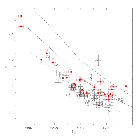
Figure 6: Run of the parameter Fe, which represents the average intensity of 17 Fe I lines in our spectra, against effective temperature. Symbols are as in Fig. 3. We overimpose three curves, representing the results obtained from a similar analysis of synthetic spectra computed with Fe abundances of [Fe/H]=-0.9, -1.1, and -1.3 (dashed, solid, and dotted lines, respectively). We note that the gravity and microturbulence of the models used for these synthetic spectra do not coincide with those appropriate for the individual stars, hence abundances cannot be derived by a simple interpolation in this plot.

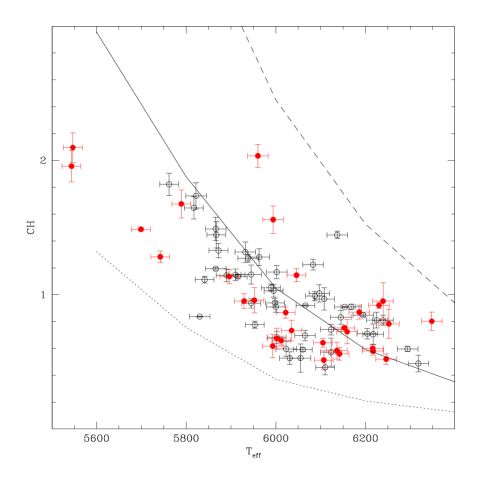
Figure 7: Similar to Fig. 6, but this time for the parameter CH, which represents the average strength of CH features within the G-band. The synthetic spectra were computed for [Fe/H]=-1.1, and [C/Fe]=-0.5, 0.0, and +0.5 (bottom to top line).

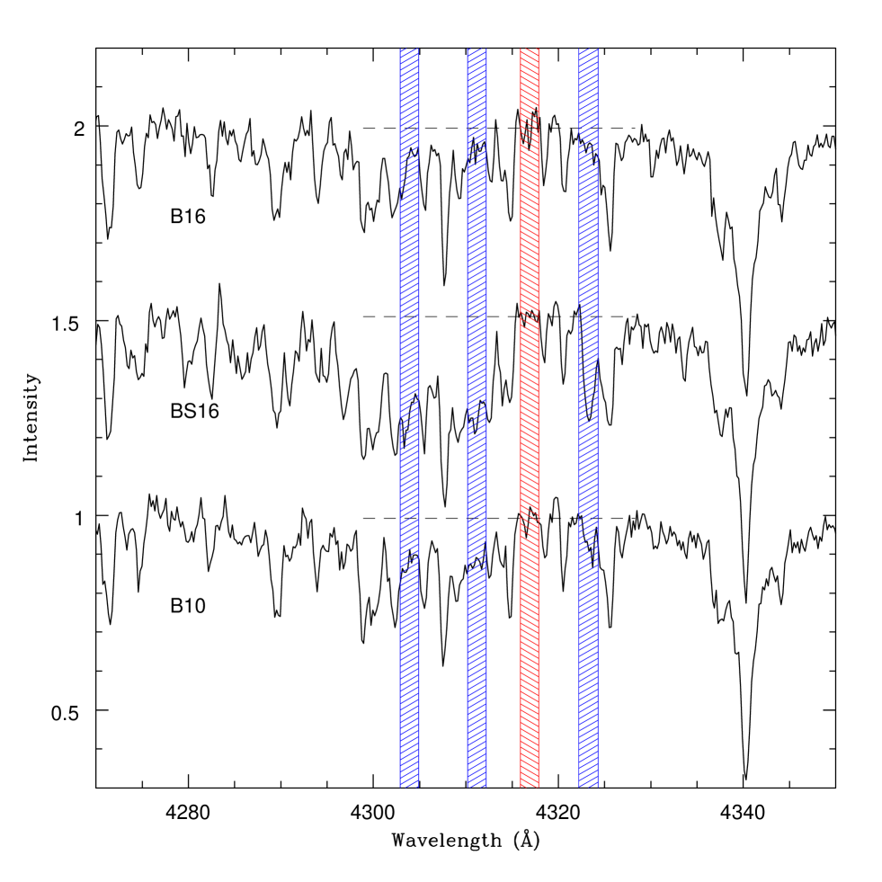
Figure 8: Spectrum in the G-band region for the C-rich star BS16 ($T_{\rm eff}=5961$ K), compared with the spectra for a C-normal star B10 ($T_{\rm eff}=5940$ K) and C-poor star B16 ($T_{\rm eff}=5985$ K). Spectra have been offset vertically for a clearer display. The spectral ranges used for the derivation of our CH index are shown as shaded areas, for easier comparison. The horizontal dashed line is at the average value within the ”continuum” reference band (4315.9-4317.9 Å).

3.2 Abundance analysis

The second step consisted in measuring abundances from these spectra. There is virtually no unblended line in the spectra of the programme stars at the adopted resolution, and nowhere do the spectra ever reach a real continuum. The usual line analysis method was then not applicable. Our approach consisted in comparing the measures of fluxes in a number of spectral bands with similar measurements made on synthetic spectra. In general, we measured fluxes in both a narrow spectral region, dominated by a strong line, and a much wider region, used to normalize the spectra in a uniform way. We considered the following atomic lines: Ali 3961.5 Å; Mgi 4057.5, 4167.3 Å; Cai 4226.7 Å; Cri 4254.3, 4289.7 Å; Mni 4030.7, 4033.1, 4034.5 Å; Fei 4045.8, 4063.6, 4071.7, 4132.1, 4143.9, 4187.0, 4202.0, 4235.9, 4250.1, 4260.5, 4271.2, 4307.9, 4325.8, 4383.6, 4404.8, 4415.1, 4528.6 Å; Srii 4077.7, 4215.5 Å; and Baii 4554.0 . This list includes all lines in the useful spectral range stronger than 200 mÅ in the solar spectrum (save for the hydrogen lines, mentioned above, and the Ca II H line, which is too strong to be measured with the present approach). For all of these lines, we measured the flux within a band 1 Å wide centred on the line, as well in a second band 21 Å wide, also centred on the line. The latter was used to provide a local reference for the line index, which ensures that observed and synthetic spectra are normalized in the same way. Figure 2 presents an example of the application of this procedure. We note that in this paper we only give results for Fe, Ca, Cr, Sr, and Ba lines. The remaining lines give inconsistent results, and should be carefully examined for possible errors in the adopted line lists.

In addition to the atomic lines, we considered three spectral bands dominated by CH lines: 4302.9-4304.9, 4310.2-4312.2, and 4322-4324.3 Å. For these features, the local reference for the line index was obtained by considering the band 4315.9-4317.9 Å, which is a relative high point in all our spectra. For examples of our spectra and the definition of these bands, we refer to Figure 8.

The synthetic spectra we computed are based on the Kurucz (1993) set of model atmospheres (with the overshooting option switched off), and line lists from Kurucz (1993) CD-ROM s, using our own synthesis code; we checked that the parameters for the strong lines contained in these lists were equal to the updated values from the VALD database (Kupka et al. 2000). The adopted solar abundances were 8.67, 6.34, 5.71, 7.63, 3.06, and 2.28 for C, Ca, Cr, Fe, Sr, and Ba, respectively, in the usual spectroscopic scale where $\log{\rm n(H)}=12.0$. There are offsets with respect to other sets of solar abundances; for instance they are up to 0.2 dex higher than those listed by Asplund et al. (2009). While some of these offsets should be applied when using different sets of model atmospheres, we underline that we are mainly interested in star-to-star abundance differences within NGC 1851, so that global offsets in the solar abundances do not affect any of the main conclusions of this paper. Synthetic spectra were computed for [A/H]=-1.6, -1.3, -1.1, -0.9 and -0.6, save for Ba, for which we adopted [A/H]=-1.0, -0.7, -0.5, -0.3, and 0.0; in this way, we virtually never need to extrapolate beyond the computed grid. The spectra were then convolved with a Gaussian having a FWHM of 0.5 Å that closely mimics the instrumental profile.

Our derivation of abundances from measured fluxes involved several steps. We wished to compute only a small set of synthetic spectra. In addition, we wished to estimates the internal errors by placing the measures for different lines on a uniform scale. In practice, this was done by dividing the integral of the residual profile measured for each line $(1-F_{\lambda})$ by its average value among all programme stars. This quantity is of the order of unity, and has a similar run with temperature for all lines of a given element because the excitation potentials of the lines are quite similar to each other, often because they belong to the same multiplet. We then averaged results for different lines of a given element; the r.m.s scatter in the individual values provides an estimate of the internal errors, which can then be used to compare abundances obtained for different stars. In practice, slightly better results were obtained by weighting the individual lines according to the scatter in the residuals with respect to the mean values. These average quantities were then compared with the results obtained by applying the same procedure to the synthetic spectra. Fig. 6 shows the results of the application of this procedure for Fe lines (we define as Fe the parameter describing the average intensity of the 17 Fe I lines that we measured on our spectra).

Fig. 7 shows similar results, this time for the parameter CH obtained considering the spectral regions close to the head of the G-band.

Abundances of the various elements in the individual stars may then be obtained by interpolations within the graphs. Rather than using interpolations, we however preferred to evaluate low order polynomials in $T_{\rm eff}$ and the various indices by least squares fitting, and then correct for gravity and microturbulence velocity appropriate for individual stars, using the sensitivities of Table 3. The abundances we obtained by this process are listed in Tables 1 and  2. For those cases in which several features were used, we also provide an internal error, which is a statistical error, and only includes the contribution due to the scatter between results obtained for different lines. Table 3 gives the sensitivity of the abundances we obtain for various elements to the the atmospheric parameters. We also list the total uncertainty, which was obtained by assuming errors of 30 K, 0.03 dex, and 0.2 km s^-1 in effective temperature, surface gravity, and microturbulence velocity, respectively. Systematic errors are much larger, of the order of 0.1 dex or more. However, insofar as they are similar among all programme stars, they do not affect our discussion.

Table 3: Sensitivity of abundances to the adopted atmospheric parameters.

Parameter	$T_{\rm eff}$	$\log{g}$	$[$A/H$]$	$v_{t}$	Total
Variation	+200 K	+0.3 dex	+0.1 dex	+0.3 km s-1
Error	30 K	0.03 dex		0.2 km s-1
$[$Fe/H$]$	+0.22	-0.18		-0.04	0.05
$[$Ca/Fe$]$	0.00	+0.02		+0.02	0.01
$[$Cr/Fe$]$	+0.14	-0.05		-0.08	0.06
$[$Sr/Fe$]$	-0.13	+0.18		-0.03	0.03
$[$Ba/Fe$]$	+0.05	+0.04		-0.09	0.05
$[$C/Fe$]$	+0.03	+0.09		+0.03	0.02
$\Delta(u-y)$	+0.078	+0.025	-0.023	-0.016	0.021
$[$N/Fe$]$	+0.98	+0.31	-0.29	-0.19	0.26

4 Abundances for individual elements

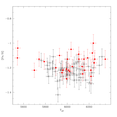
Figure 9: Run of the abundance of Fe with effective temperature. Symbols are similar to those in Fig. 3

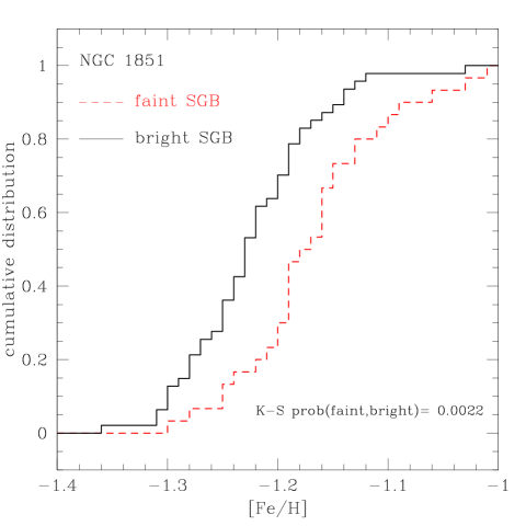
Figure 10: Comparison between the cumulative distribution of [Fe/H] values for b-SGB and f-SGB stars. We also show the result of the application of the Kolmogorov-Smirnov test to determine the probability that the two distributions were extracted from the same parent population.

4.1 Iron

Fig. 9 gives the run of the abundance of Fe with the effective temperature. No trend with temperature is present. On average, we obtain [Fe/H]=$-1.20\pm 0.01$ (r.m.s.=0.07 dex). This value compares very well with recent determinations of the metal abundance of NGC 1851, as summarized in Table 4.

Table 4: Fe abundance in NGC 1851 for different groups of stars

Group	N. stars	[Fe/H]	r.m.s.	paper
SGB	77	$-1.20\pm 0.01$	0.07	This paper
SGB-b	47	$-1.23\pm 0.01$	0.06	This paper
SGB-f	30	$-1.16\pm 0.01$	0.07	This paper
Upper RGB	13	$-1.18\pm 0.02$	0.07	Carretta et al. (2010c)
Upper RGB	121	$-1.15\pm 0.01$	0.05	Carretta et al. (2011a)
RHB	55	$-1.14\pm 0.01$	0.06	Gratton et al. (2012b)
Lower RGB	13	$-1.18\pm 0.03$	0.11	Gratton et al. (2012b)

All of these sets of abundances were obtained using the Alonso et al. (1996, 1999) temperature scales (the BASTI one in the present paper), the Kurucz (1992) model atmospheres, and local thermodynamic equilibrium. The [Fe/H] value we get for the b-SGB is lower (by 0.08 dex) than the value obtained for the RHB, in spite of their being likely to belong to the same population. This difference is much larger than the statistical errors (those listed in Table 4) and might perhaps agree with expectations for the impact of sedimentation. However, we are not inclined to attribute much importance to this difference, given the potential offsets that can be present for these different analyses. We propose instead that this comparison may give the reader a clearer idea of the uncertainties that exist in the zero points of these different abundance determinations other than the statistical errors.

Stars on the f-SGB have systematically higher Fe abundances than those on the b-SGB. On average, we have [Fe/H]=$-1.227\pm 0.009$ for the b-SGB stars, and [Fe/H]=$-1.162\pm 0.013$ for the f-SGB. The r.m.s. scatter in the abundances of 0.062 dex and 0.071 dex, respectively, can be attributed to a combination of the effects of the line-to-line scatter ($\sim 0.04$ dex: see Tables 1 and  2) and the internal errors in the atmospheric parameters ($\sim 0.05$ dex, see Table 3). The difference between the average Fe abundances of the b-SGB and f-SGB is significant at more than 4$\sigma$: it cannot be attributed to a random fluctuation. This is clearly shown by Figure 10, where we compared the cumulative distributions of [Fe/H] values for b-SGB and f-SGB stars. An application of the Kolmogorov-Smirnov test to determine the probability that the two distributions were extracted from the same parent population returns a very low value of 0.0022. In addition, the difference cannot be explained by errors in the adopted masses: to eliminate this difference, we would have to assume that the mass of f-SGB stars is  20% higher than the value for the b-SGB stars, which does not sound reasonable (if anything, we would expect that the masses of f-SGB stars are lower, not higher than those of b-SGB stars, and in any case the difference should be very small, $<2$%). We are then inclined to conclude that there is a real difference between the metal abundances of f-SGB and b-SGB. We note that Carretta et al. (2010c, 2011a) also concluded that there is a real range of metal abundances in NGC 1851, while Villanova et al. (2010) did not find any difference when stars were divided into groups according to their Strömgren indices. This might be understood if - for the upper RGB - the subdivision of stars into groups given by Strömgren photometry did not exactly reproduce that in b-SGB/f-SGB.

We note that there appear to be a couple of outliers in Figure 6. The most discrepant case is star AS57, which we actually omitted from Table 1. Its Fe index would correspond to [Fe/H]=-0.72. Inspection of the spectrum confirms that this star has stronger lines than the other stars of similar $T_{\rm eff}$. In the theoretical $T_{\rm eff}$-gravity diagram of Figure 5, this star ($T_{\rm eff}$=6137, $\log{g}$=3.936) corresponds to the most discrepant data point having too low a gravity for its adopted $T_{\rm eff}$. Our assumed $T_{\rm eff}$ might indeed be overestimated; if we adopt $T_{\rm eff}$ from $(B-I)$ colour ($T_{\rm eff}$=6004 K), we have $\log{g}$=3.895, in agreement with the values inferred for other stars of similar $T_{\rm eff}$. However, the [Fe/H] value ([Fe/H]=-0.89) would still differ by more than five standard deviations from the values for other b-SGB stars and again a direct comparison shows that the observed iron lines are much stronger than for other stars of even this lower temperature. The $T_{\rm eff}$ that would be required to recover a typical [Fe/H] value is $\sim 5700$ K, but this would be excluded by both the spectrum and the photometry. An alternative possibility is that this star is actually a binary (either real or apparent).

The next possible outlier in Figure 6 is star BS19, which is the warmest in our sample. However, in this case there is no real anomaly, and the apparent discrepancy is simply caused by the adopted values for $\log{g}$ and $v_{t}$ for this star which considerably differ from those used to draw the lines in Figure 6.

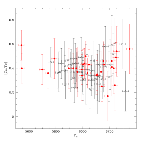
Figure 11: Run of the [Ca/Fe] abundance ratio with effective temperature. Symbols are similar to those in Fig. 3

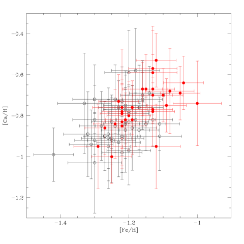
Figure 12: Comparison between [Ca/H] and [Fe/H]. Symbols are similar to those in Fig. 3

4.2 Calcium

Fig. 11 shows the run of the [Ca/Fe] ratio with effective temperature. This run is uniform and flat at [Ca/Fe]=$0.40\pm 0.01$, with an r.m.s.=0.09 dex. While this result is expected to be almost independent of the choice of the atmospheric parameters, the scatter still appears remarkably small for an abundance based on a single line in moderately low resolution spectra. The average value is similar to those derived by Carretta et al. (2010c, 2011a: [Ca/Fe]=$0.30\pm 0.02$) and Gratton et al. (2012b: [Ca/Fe]=0.42) from an analysis of RGB and RHB stars, respectively.

Fig. 12 compares the abundances of Fe and Ca. This figure clearly shows that both Fe and Ca are more abundant in f-SGB than in b-SGB stars. We found average abundances of [Ca/H]=$-0.836\pm 0.014$ for b-SGB stars, and [Ca/H]=$-0.756\pm 0.020$ for f-SGB stars. This implies that large differences in Ca/Fe would be unable to explain the spread in $Cauvby$ photometry noted by Lee et al. (2009). This agrees with the discussions of Carretta et al. (2010b) and Sbordone et al. (2011).

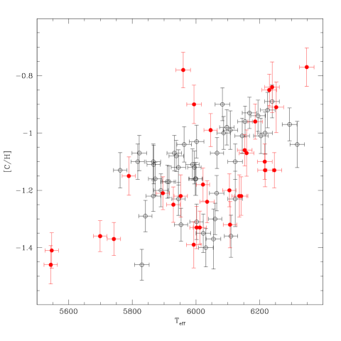
Figure 13: [C/H] ratio as a function of effective temperature. Symbols are similar to those in Fig. 3

4.3 Carbon

Fig 13 displays the run of [C/H] with effective temperature. This plot is very instructive and is worthy a closer examination. We begin by considering the b-SGB star. First, we note that there is a clear overall trend for decreasing C abundances with decreasing temperature, with a slope of about 0.0005 dex/K. This small trend could possibly be due to the deepening of the convective envelope when the star moves from the main-sequence turn-off to the base of the RGB. Furthermore, the distribution appears skewed, with a group of 27 stars that define a very narrow relation (r.m.s. of 0.033 dex, excluding one star that has a slightly higher than average C abundance) at the upper envelope of the distribution, the remaining 19 stars scattering below, within a range of about 0.4 dex. We might expect that the C-normal group are N-poor, and the C-poor stars are N-rich; unluckily, the CN band at 4216 Å is too weak to confirm this difference. The distribution of f-SGB stars appears to be more scattered, the stars being on average a little poorer in C than the b-SGB stars. However, this large scatter may be caused by the stars of C-normal and C-poor groups having different distributions, rather than a general property of all stars. This can be shown by comparing the offsets in C abundances from a mean line representing the bulk of b-SGB stars, as represented by the equation:

$${\rm offset[C/H]}={\rm[C/H]}-[0.0005\leavevmode\nobreak\ (T_{\rm eff}-6200)-0.965]$$ (1)

We may then separate C-normal stars from C-poor stars at a [C/H] value that is that given by the relation minus twice the r.m.s. of the bulk of b-SGB stars around the relation itself; that is, C-normal stars have offset[C/H]$>-0.067$, while C-poor stars have offset[C/H]$<-0.067$. Among b-SGB stars, there are 27 C-normal stars, 17 C-poor stars, and 1 star slightly more C-rich than the C-normal ones. Among the f-SGB stars, there are 22 C-poor stars, 3 C-normal stars, and 5 C-rich stars. The very different incidences of C-rich, C-normal, and C-poor stars among the two populations is remarkable.

As mentioned above, the spectra of a few stars contain a G-band that is definitely stronger than in the remaining spectra; an example is shown in Figure 8, where we compare a spectrum of the f-SGB star BS16 with that of two other f-SGB stars of similar temperature (B10 and B16). There is little doubt that the G-band is indeed stronger in the first star. The C abundances we derived using our procedure are [C/Fe]=$+0.43\pm 0.03$ for BS16, $0.02\pm 0.05$ for B10, and $-0.20\pm 0.05$ for B16. In our opinion, these C-rich stars are most likely the progenitors of the stars on the anomalous RGB branch in the $v,(v-y)$ diagram, for the reasons that we discuss below.

Finally, Lardo et al. (2012) analysed the C and N contents of a quite large number of stars close to the subgiant branch of NGC 1851. A comparison with their results is needed. However, not only are there only three stars in common between the samples, but we also note that these authors attributed an effective temperature of about 5850 K to the turn-off stars of NGC 1851. This is about 500 degrees cooler than expected for the BASTI group isochrones (Pietrinferni et al. 2006) they used elsewhere in their paper. The main effect of such a low temperature scale on their analysis is to severely underestimate the abundances of C, which are indeed very low with typical values of [C/Fe]$\sim-0.6$. In turn, this yields too low C+N abundances for the C-normal, N-poor stars, which are predominant on the b-SGB but are only a minority of the f-SGB stars (see Section 4.3), and leads to the authors’ conclusion about the difference between the sum of C+N abundances for the two branches. Furthermore, the large scatter that is clearly evident in a star-to-star comparison among the only three stars in common between the two samples induces us to suspect that they underestimated the impact of their observational errors on their C abundances. Since N abundances are derived from CN bands, any error in the C abundances propagates into the N ones, creating a spurious C-N anticorrelation.

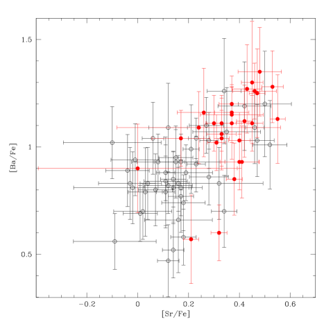
Figure 14: Comparison between [Sr/Fe] and [Ba/Fe] abundance ratios. Symbols are similar to those in Fig. 3

Figure 15: Hess diagram constructed for the [Sr/H] and [Ba/H] abundance ratios. Crosses indicate the mean Sr and Ba contents of the two bumps with their internal errors.

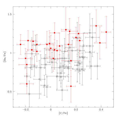
Figure 16: Correlation between the Ba and C abundances. Symbols are similar to those in Fig. 3

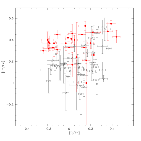
Figure 17: Correlation between Sr and C abundances. Symbols are similar to those in Fig. 3

4.4 Neutron-capture elements

We measured abundances for two n-capture elements (Sr and Ba). Both elements are mainly produced by the s-process in the solar system. Fig. 14 and 15 compare the abundances of Sr and Ba. These plots show two interesting features:

• Both Sr and Ba are more abundant in f-SGB than b-SGB stars. The differences are $\Delta$[Sr/Fe]=$0.19\pm 0.03$ dex and $\Delta$[Ba/Fe]=$0.20\pm 0.04$ dex. Differences are even larger in [Sr/H] and [Ba/H] ($0.25\pm 0.03$ and $0.26\pm 0.04$, respectively).

• In both groups, there is a clear correlation between [Sr/Fe] and [Ba/Fe], suggesting that there is a real spread in the abundances of n-capture elements. This agrees with the correlation found for RGB and RHB stars, if we identify RHB stars with b-SGB ones.

• Both Sr and Ba have bimodal distributions as previously noticed by Villanova et al. (2010). This bimodality is visible in both Figures 14 but is more clearly evident in Fig. 15, where we present a Hess diagram of the [Ba/H] versus [Sr/H] relation. Two clear bumps are visible. Two crosses indicate the mean Sr and Ba content of the two bumps with their internal errors. The bimodality of $s-$elements (both light and heavy) in NGC 1851 obtained by Villanova et al. (2010) appears to be definitely proven, although there are offsets between the mean abundances of the two groups of stars that may depend on the differences between the analysis methods.

• If we consider the distribution of stars in the SGB (Fig. 1), the [C/H] vs T_eff diagram (Fig. 13), and the [Ba/H] vs. [Sr/H] diagram (Fig. 15), we see that there is no one-to-one relation among these quantities. For example, both branches are populated by C-normal and C-poor stars, while not all stars that are Ba-rich are also C-poor and viceversa. Measurement errors are clearly responsible for part of these perplexing results, but the lack of correlation can be hardly entirely justified in this way.

We then looked for a correlation between n-capture elements and C abundances (see Fig. 16 and 17). There is some correlation for Ba, while the result for Sr is much more dubious. However, both results might be influenced by the small trends with effective temperatures.

Finally, we note that Sr and Ba abundances for the few C-rich stars are slightly higher than for the other stars, but the difference is not large. Typical values are [Sr/Fe]$\sim 0.45$ and [Ba/Fe]$\sim 1.25$, that are $\sim 0.3$ dex higher than average.

5 Nitrogen abundances

Clearly, CNO abundances play a very special role in NGC 1851. We now examine the evidences for N abundances determined for the stars we observed. Unfortunately, we do not have any N abundance indicator in our spectra because the CN band at 4216 Å is too weak in the programme stars. In these warm stars, the best indicator of N is the NH band. While we have no spectroscopic data at the relevant wavelengths, we have Strömgren photometry for most of the stars. We tried several combinations of the Strömgren indices and found that best results are obtained using $u-y$, where the $u$-band is affected by NH and CN lines, which are not present in the $y$-band. Since $u-y$ is both temperature and gravity dependent, we should use the offset from an average relation of this index against temperature. We called this offset $\Delta(u-y)$, whose definition is:

$$\Delta(u-y)=(u-y)-(0.0005708\leavevmode\nobreak\ T_{\rm eff}-5.056).$$ (2)

Values for individual stars are given in the last column of Table 1.

As an exercise, we then synthesized Strömgren colours for subgiants with different N-contents. We adopted a similar approach to Carretta et al. (2011b; see also Sbordone et al. 2011 for a similar discussion). We found that a huge excess of N, say [N/Fe]=1.5 (2.0), shifts the $u-y$ colour by as much as 0.10 (0.16) mag, with virtually no effects on all bands apart from $u$ (the test was done for $T_{\rm eff}=6000$ K, which is typical of the programme stars). Of course, $\Delta(u-y)$ also depends on other parameters (temperature, gravity, Fe abundance, and microturbulence velocity). We explored this dependence by modifying these parameters in the synthesis, and estimating the impact on $\Delta(u-y)$. The relevant values are given in Table 3, in terms of the effects of variation of the parameters on both $\Delta(u-y)$ and the [N/Fe] values that we would infer from these data. While the sensitivities are not at all negligible, the accuracy of our determination of the atmospheric parameters ensures that the internal errors in $\Delta(u-y)$ and [N/Fe] are dominated by the photometric errors.

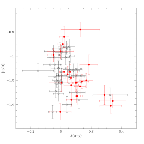
Figure 18: Correlation between $\Delta(u-y)$ and C abundances. Symbols are similar to those in Fig. 3

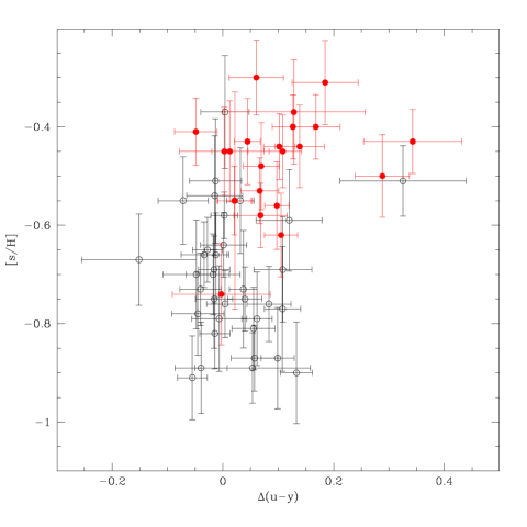
Figure 19: Correlation between $\Delta(u-y)$ and the average of Sr and Ba abundances. Symbols are similar to those in Fig. 3

In Figures 18 and 19, we then compared the $\Delta(u-y)$ with [C/H] and [s/H]=[(Sr+Ba)/H] abundances. Although the scatter is quite large, owing to the photometric errors, $\Delta(u-y)$ is positively correlated with [s/H] and anticorrelated with [C/H] for the f-SGB stars, while the results are less clear for b-SGB ones. This is reasonable because $\Delta(u-y)$ may be considered as a measure of the N abundance (even though with large errors). To quantify these effects, we performed various tests.

We first estimated the average values of $\Delta(u-y)$ in both groups of SGB stars. We obtained values of $0.021\pm 0.013$ mag (35 stars, r.m.s.=0.078 mag) and $0.101\pm 0.021$ mag (24 stars, r.m.s.=0.103 mag) for the b-SGB and f-SGB stars, respectively. There is then a systematic difference of $0.080\pm 0.024$ mag between the two groups, which is significant at more than the 3-$\sigma$ level. This offset is much larger than expected for the tiny differences in gravity and metal abundances (which can justify only about one fifth of the difference), and should then be real and likely related to a difference in the average N content. We would then expect f-SGB stars to have on average a [N/Fe] which is $\sim 1.0$ dex higher than that of b-SGB stars. Since we find a large difference in the fraction of C-poor stars, this higher abundance is likely due to a much larger incidence of N-rich stars. This closely agrees with the lower average [C/Fe] values obtained for the f-SGB stars, in the framework of an anticorrelation between C and N abundances.

Second, such an anticorrelation is evident when directly examining the results for individual stars. We estimated the linear correlation coefficient between [C/H] and $\Delta(u-y)$, and found a value of r=0.331 (59 stars, $<0.005$ probability to be a random result) when considering all stars. The correlation coefficient is insignificant for the b-SGB stars alone (r=0.136 over 35 stars), while it is quite high (r=0.458 over 24 stars) for f-SGB stars alone ($\sim 0.02$ probability of being a random result).

We conclude that there is a significant anticorrelation between [C/H] and $\Delta(u-y)$, which is mainly driven by the f-SGB stars. These results may indicate that most b-SGB stars are C-normal and N-normal; while the majority of f-SGB ones are C-poor and N-rich.

We note that there is a small group of four (three on the f-SGB and one on the b-SGB) stars that have very large values of $\Delta(u-y)\sim 0.3$. Given their high N abundances, these stars might be considered potential progenitors of the stars on the anomalous RGB branch in the $v,(v-y)$ diagram instead of the C-rich stars mentioned above. However, we first note that with an average [Ba/Fe]=0.32 these stars do not have a large overabundance of Ba, which is an important characteristic of the stars on the anomalous RGB branch (Villanova et al. 2010; Carretta et al. 2011b). Secondly, such a large $\Delta(u-y)$ value, if naively interpreted in terms of anomalous N overabundances, would produce a huge value of [N/Fe]$>>2$. We deem that it is more likely that the large values of $\Delta(u-y)$ found for these stars is due to a combination of high (but not exceptional) N abundances with observational errors (errors shown in Figures 18 and 19 are the internal errors in the photometry, and may underestimate real errors in case of blends). Ultraviolet spectra of these stars would of course be extremely helpful.

We may compare this result with that of Lardo et al. (2012) mentioned in the introduction. Unsurprisingly, we found a very good correlation between $\Delta(u-y)$ used throughout this paper and the residuals around the mean relation between the index used by Lardo et al. ($(u-y)+(v-b)$) and V magnitudes for the SGB.

Finally, we note that C-rich stars have small values of $\Delta(u-y)$, which are indicative of normal (low) N abundances. Their composition suggests that they formed from material polluted by the products of triple-$\alpha$ reactions.

6 Discussion and conclusions

A short summary of the results of our analysis is as follows:

• We have been able to clearly distinguish between the b-SGB and f-SGB populations of NGC 1851 in the theoretical $T_{\rm eff}-\log{g}$ diagram.

• We have found a small but significant difference in the metal abundances. The b-SGB has [Fe/H]=$-1.23\pm 0.01$, while for the f-SGB we obtained [Fe/H]=$-1.16\pm 0.01$. Hence, the f-SGB is slightly more metal-rich than the b-SGB. The sense of this difference is the same as that found by Marino et al. (2012b) for M 22.

• If we then assumed the same He and CNO/Fe ratios for the two populations, the difference in age between them is reduced to 0.6 Gyr only. The analysis of the HB performed in Gratton et al. (2012b) shows that the BHB (which is likely mostly populated by the progeny of the f-SGB population) is slightly more He-rich (Y$\sim$0.29 vs. Y$\sim$0.25) than the RHB (which is likely the progeny of the b-SGB population). However, detailed comparisons with isochrones computed for this purpose shows that this conclusion about the age difference is unaffected by modifications of the He abundances (which however affect the masses of the stars). On the other hand, CNO abundances are much more a concern. If for instance we assume that the sum of C+N+O is larger by a factor of 2 for f-SGB stars than b-SGB stars, then the first would be found to be younger than the second by $\sim 0.4$ Gyr, which is almost exactly the opposite of what we get by assuming the same CNO/Fe ratio. This would of course completely change the evolutionary scenario appropriate to interpreting our observations.

• The variation in Fe abundances is paired by abundances in other elements such as Ca, that is the [Ca/Fe] ratio is very similar in the two populations.

• The neutron-capture elements Sr and Ba show much larger differences between the b-SGB and the f-SGB than Fe or Ca. These elements have a strong bimodality, as found by Villanova et al. (2010). This result is again similar to that found by Marino et al. (2012b) for M 22.

• Both the b-SGB and the f-SGB stars exhibit a spread in C abundances (this result coincides with that of Lardo et al. 2012), but the ratio of C-normal to C-poor stars are very different in the two populations: they are 27:17 and 3:22 for the b-SGB and f-SGB, respectively.

• We were unable to derive N abundances from our spectra. When we assumed that an index $\Delta(u-y)$ derived from Strömgren photometry provides information about the N abundance, we found that there is a quite good C-N anticorrelation for the f-SGB, while results are unclear for the b-SGB. In addition, we found that on average the f-SGB stars are more N-rich than b-SGB stars. This is likely related to the very different incidence of C-normal and C-poor stars in the two groups.

• There are a few abnormally C-rich stars, most of them (five out of six) in the f-SGB. The C overabundance of these stars is obvious even from a simple inspection of the spectra. These stars are also Sr- and Ba-rich, though there appears to be other stars in the cluster with comparable Sr and Ba abundances. We propose that these stars are the most likely progenitors of the stars on the anomalous RGB in the $v-(v-y)$ diagram, since (i) a high C abundance might be an explanation for the anomalous $v-y$ colours (Carretta et al. 2010c), (ii) these stars are Ba-rich, and (iii) the number of observed C-rich stars (6 out of 78) is in reasonable agreement with the fraction of RGB stars on the anomalous RGB. We note that the N-abundance of the C-rich stars is similar to the average for the other stars, suggesting that they owe their large C-abundance to triple-$\alpha$ reactions in the progenitor population and not to hot bottom burning.

Combining all evidences cumulated so far, it is clear that NGC 1851 has had a complex history, as we also concluded in our previous analyses of the RGB (Carretta et al. 2010b 2011a) and HB (Gratton et al. 2012b). The results obtained throughout this paper might be interpreted in a scheme where NGC 1851 is the result of the merging of two globular clusters, as suggested by Van den Bergh (1996), Catelan (1997), and Carretta et al. (2010c, 2011a). This might explain why we found separate O-Na anticorrelations along the RHB and the BHB, and C-N anticorrelations along the b-SGB and f-SGB (see also Lardo et al 2012). The apparent inconsistency that the older sequence is more metal-rich than the younger one can be understood if NGC 1851 formed within a chemical inhomogeneous structure and the two populations originated in different regions of this parent object. However, it is also possible that there is a precise relation between these two episodes of star formation. The two most well-studied clusters exhibiting a spread in their subgiant branches, NGC 1851 and M 22, share a surprisingly long list of common features. In both cases, (i) the f-SGB appears more metal-rich than the b-SGB; (ii) they have similar [Ca/Fe] ratios; (iii) assuming a constant C+N+O, the age difference is about 0.5-0.6 Gyr; (iv) spreads in the abundances of C and N (at least) are present among both SGBs, with on average more N residing in the f-SGB stars (either owing to a larger fraction of N-rich stars or to a larger CNO content); and (v) n-capture elements are overabundant in the f-SGB relative to the b-SGB. It may well be that this long list of coincidences is not due only to chance, but they are also consistent with both NGC 1851 and M 22 being simply the result of the merging of two globular clusters that formed independently.

Figure 20: Difference between the best-fit ages for the b-SGB and f-SGB of NGC 1851 as a function of the assumed difference in CNO abundance $\delta$CNO between the two populations.

A crucial piece of information concerns the sum of C+N+O abundances. The difference in the ratio (C+N+O)/Fe does not need to be huge to have an important impact on this scenario: a mere difference of a factor of two in the sum of C+N+O abundances between b-SGB and f-SGB makes the latter actually younger than the first (see Figure 20). In this case, we might possibly devise a scenario where a sequence of star formation episodes related to each other in a causal way generates all populations observed in both NGC 1851 and M 22. In this case, an important role is likely played by nucleosynthesis in stars with a mass of 2.5-4 $M_{\odot}$ that might explain the abundance pattern of C-rich stars. Unfortunately, when we need to sum the abundances of different elements, we must consider absolute -not simply differential- abundances. Absolute abundances are much more sensitive to systematic errors, which can significantly affect the conclusion drawn. Perhaps unsurprisingly, the most recent results in the literature lack consensus. Various authors (Yong and Grundahl 2008; Yong 2011) found that there is a real difference in the ratio (C+N+O)/Fe, though their results can actually appear to be quite different depending on the observable that is used. On the other hand, no difference was found by Villanova et al. (2010), and a quite low upper limit was obtained by Gratton et al. (2012b).

The most easily observed stars are of course those on the RGB. Unfortunately, their atmospheres are quite poorly understood, and the absolute abundances that have been determined for these stars are likely uncertain at a level possibly unacceptable in this context. In addition, the distinction between the RGB progeny of b-SGB and f-SGB stars is not easy. A more robust determination of N abundances as well as a completely new determination of O abundances for dwarfs and subgiants in NGC 1851 would clearly be highly welcome because it would enable us to derive this badly needed datum. The use of CN bands, though observationally easier, is difficult, because if our errors in C abundances are underestimated, a spurious C-N anticorrelation can appear. It is unclear whether this is the case for the C-N anticorrelation found by Lardo et al. (2012), which might also be real. However, the use of an abundance indicator that is completely independent of C abundances, such as the NH bands in the near UV is in our opinion preferable.

Finally, we propose that a detailed spectroscopic study of the HB of M 22 should be performed, in order to understand whether there is also bimodality as in the case of NGC 1851, and to derive He abundances at least for some stars, as was done in M 4 by Villanova et al. (2012).

- (1) Alonso, A., Arribas, S., Martinez-Roger, C. 1996, A&A, 313, 873
- (2) Alonso, A., Arribas, S., & Martinez-Roger, C. 1999, A&A, 140, 261
- (3) Alves-Brito, A., Yong, D., Meléndez, J., Vásquez, S., Karakas, A.I. 2012, A&A, in press (arXiv:2012.0797)
- (4) Asplund, M., Grevesse, N., Sauval, A.J., Scott, P. 2009, ARA&A, 47, 481
- (5) Bekki, K, Yong, D. 2012, MNRAS, 419, 2063
- (6) Bellazzini, M., Bragaglia, A., Carretta, E., et al. 2012, A&A, 538, 18
- (7) Carretta, E., Gratton, R.G., Lucatello, S., Bragaglia, A., Bonifacio, P. 2005, A&A, 433, 597
- (8) Carretta, E., Bragaglia, A., Gratton, R. G., et al., 2010a, A&A, 516, 55
- (9) Carretta, E., Bragaglia, A., Gratton, R. G., et al., 2010b, ApJ, 712, L21
- (10) Carretta, E., Gratton, R.G., Lucatello, S., et al. 2010c, ApJ, 722, L1
- (11) Carretta, E., Lucatello, S., Gratton, R.G., Bragaglia, A., D’Orazi, V. 2011a, A&A, 533, 69
- (12) Carretta, E., Bragaglia, A., Gratton, R., D’Orazi, V., Lucatello, S. 2011b, A&A, 535, 121
- (13) Cassisi, S., Salaris, M., Pietrinferni, A., et al. 2008, ApJ, 672, L115
- (14) Catelan, M. 1997, ApJ, 478, L99
- (15) Catelan, M., Borissova, J., Sweigart, A.V., Spassova, N. 1998, ApJ, 494, 265
- (16) Decressin, T., Meynet, G., Charbonnel, C., Prantzos, N., Ekstr m, S. 2007, A&A, 464, 1029
- (17) Ferraro, F.R., Dalessandro, E., Mucciarelli, A. et al. 2009, Nature, 462, 483
- (18) Gratton, R.G., Carretta, E., Castelli, F. 1996, A&A, 314, 191
- (19) Gratton, R.G., Bonifacio, P., Bragaglia, A., et al. 2001, A&A, 369, 87
- (20) Gratton, R.G., Sneden, C., Carretta, E. 2004, ARA&A, 42, 385
- (21) Gratton, R.G., Carretta, E., Bragaglia, A., Lucatello, S., D’Orazi, V. 2010, A&A, 517, 81
- (22) Gratton, R.G., Carretta, E., Bragaglia, A., 2012a, A&AR, in press (arXiv:1201.6526)
- (23) Gratton, R.G., Lucatello, S., Carretta, E., et al. 2012b, A&A, 539, 19
- (24) Grundahl, F., Catelan, M., Landsman, W.B., Stetson, P.B., Andersen, M.I. 1999, ApJ, 524, 242
- (25) Han, S.-I, Lee, Y.-W., Joo, S.-J. et al., 2009, ApJ, 707, L190
- (26) Harris, W.E., 1996, AJ, 112, 1487
- (27) Kraft, R.P. 1994, PASP, 106, 553
- (28) Kupka F., Ryabchikova T.A., Piskunov N.E., Stempels H.C., Weiss W.W., 2000, Baltic Astronomy, 9, 590
- (29) Kurucz, R.L. 1993, CD-ROM 13, Smithsonian Astrophysical Observatory, Cambridge
- (30) Lardo, C., Milone, A.P., Marino, A.F. et al. 2012, A&A, in press (arXiv:1202.6176)
- (31) Lee, J. W., Kim, S.-L., Lee, C.-U., Youn, J.-H. 2009, Nature, 462, 480
- (32) Marin-Franch, A., Aparicio, A., Piotto, G. et al. 2009, ApJ, 694, 1498
- (33) Marino, A.F., Sneden, C., Kraft, R.P. et al., 2011, A&A, 532, 8
- (34) Marino, A.F., Milone, A. P.; Sneden, C., 2012, A&A, in press (arXiv:1202.2825)
- (35) Milone, A.P., Bedin, L.R., Piotto, G., et al. 2008, ApJ, 673, 241
- (36) Milone, A.P., Bedin, L.R., Piotto, G., & Anderson, J. 2009, A&A, 497, 755
- (37) Origlia, L., Rich, R.M., Ferraro, F.R., et al. 2011, ApJ, 726, L20
- (38) Pasquini, L., Castillo, R., Dekker, H. et al. 2004, SPIE, 5492, 136
- (39) Pietrinferni, A., Cassisi, S., Salaris, M., Castelli, F. 2006, ApJ, 642, 797
- (40) Piotto, G. 2009, IAU Symp., 258, 233
- (41) Roederer, I.U., Marino, A.P., Sneden, C., 2011, ApJ, 742, 37
- (42) Sbordone, L., Salaris, M., Weiss, A., Cassisi, S., 2011, A&A, 534, 9
- (43) Scarpa, R., Marconi, G., Carraro, G., Falomo, R., Villanova, S. 2011, A&A, 525, 148
- (44) van den Bergh, S. 1996, ApJ, 471, L31
- (45) Ventura, P., D Antona, F., Mazzitelli, I., & Gratton, R. 2001, ApJ, 550, L65
- (46) Ventura, P., Caloi, V., D’Antona, F. et al. 2009, MNRAS, 399, 934
- (47) Villanova, S., Geisler, D., & Piotto, G. 2010, ApJ, 722, L18
- (48) Villanova, S., Geisler, D., Piotto, G., & Gratton, R.G., 2012, ApJ, 748, 62
- (49) Walker, A.R. 1992, PASP, 104, 1063
- (50) Yong, D., & Grundahl, F. 2008, ApJ, 672, L29
- (51) Yong et al. 2011, in press