Time evolution of a thin black ring via Hawking radiation

Abstract

Black objects lose their mass and angular momenta through evaporation by Hawking radiation, and the investigation of their time evolution has a long history. In this paper, we study this problem for a five-dimensional doubly spinning black ring. The black ring is assumed to emit only massless scalar particles. We consider a thin black ring with a small thickness parameter, $\lambda\ll 1$, which can be approximated by a boosted Kerr string locally. We show that a thin black ring evaporates with fixing its thickness parameter $\lambda$. Further, in the case of an Emparan-Reall black ring, we derive analytic formulas for the time evolution, which has one parameter to be evaluated numerically. We find that the lifetime of a thin black ring is shorter by a factor of $O(\lambda^{2})$ compared to a five-dimensional Schwarzschild black hole with the same initial mass. We also study detailed properties of the Hawking radiation from the thin black ring, including the energy and angular spectra of emitted particles.

I Introduction

In four spacetime dimensions, a stationary, asymptotically flat, vacuum black hole is completely characterized by its mass and spin angular momentumCarter:1971zc . In particular, the topology of its event horizon must be a sphere Hawking:1971vc . By contrast, in five dimensions, in addition to the Myers-Perry black hole Myers:1986un which is a natural generalization of the four-dimensional Kerr black hole, various exact solutions of black objects with nonspherical horizon topologies have been found (see Emparan:2008eg for a review). In this paper, we focus attention to black ring solutions with the $S^{1}\times S^{2}$ horizon topology. A black ring solution rotating in the direction of $S^{1}$ was found by Emparan and Reall Emparan:2001wn . Since a five-dimensional spacetime can have two angular momenta, Pomeransky and Sen’kov Pomeransky:2006bd extended it to a solution with two independent rotation parameters (i.e., spinning both in the directions of $S^{1}$ and $S^{2}$).

A black hole is known to evaporate due to quantum effects of fields in curved spacetime as shown by Hawking Hawking:1974sw . The rate of mass and angular momentum loss by the Hawking radiation for a Kerr black hole was first studied by Page Page:1976df ; Page:1976ki taking account of fields with spins 1/2, 1, and 2, and it was shown that a Kerr black hole spins down to a nonrotating black hole regardless of its initial state. However, Chambers et al. Chambers:1997ai (see also Taylor:1998dk ) showed that if only a massless scalar field is taken into account (i.e., in the absence of fields with nonzero spin), a four-dimensional Kerr black hole evolves to a state with the nonvanishing nondimensional rotation parameter, $a/M\simeq 0.555$. This analysis was extended to five-dimensional Myers-Perry black holes by Nomura et al Nomura:2005mw . They showed that any such black hole with nonzero rotation parameters $a$ and $b$ evolves toward an asymptotic state with $a/M^{1/2}=b/M^{1/2}\simeq 0.1975(8/3\pi)^{1/2}$. Here, this value is independent of the initial values of $a$ and $b$.

It is interesting to extend these studies to the case of a black ring. Although the Hawking radiation of black rings has been studied in various context Miyamoto:2007 ; Chen:2007 ; Zhao:2006 ; Jiang:2008 , the time evolution of a black ring has not been studied up to now. The difficulty in this study is that the method of mode decomposition of the Klein-Gordon field in this spacetime is not known since separation of variables has not been realized, and therefore, two-dimensional numerical calculations of eigenfunctions are required. In order to avoid this difficulty, we consider a thin black ring with a small thickness parameter, $\lambda\ll 1$. Here, “thin” or the small thickness parameter $\lambda$ means that the $S^{2}$ radius is much smaller compared to the $S^{1}$ radius. In such a situation, a black ring can be approximated by a boosted black string. Then, the separation of variables for the scalar field can be done, and we have well defined modes.

Using this thin-limit approximation, we give a formulation to study the evolution of a thin Pomeransky-Sen’kov black ring by the Hawking radiation, and discuss general features that do not depend on details of the greybody factor. Then, we apply our method to a special case of the Emparan-Reall black ring without $S^{2}$ rotation, and derive a semi-analytic formula for the time evolution of the evaporation. Here, the formula is semi-analytic in the sense that the evolution is expressed by analytic formulas but they include one parameter related to the greybody factors that have to be evaluated numerically. By developing a numerical code, we also determine the value of this parameter with sufficient numerical accuracy.

In addition to the time evolution, we present numerical results on detailed properties of the evaporation of a thin Emparan-Reall black ring. Specifically, we examine the energy and angular spectra of emitted particles in the evaporation. In order to clarify the property of the energy spectrum that is specific to the evaporation of a black ring, we discuss the results by comparing it with that of a four-dimensional Schwarzschild black hole.

This paper is organized as follows. In Sec. II, the black ring solution is reviewed and its boosted Kerr string limit is shown. In Sec. III, we derive the equations that determine the emission rates of mass and angular momenta of a black ring via Hawking radiation. In Sec. IV, the time evolution of an evaporating black ring is studied. In Sec. V, we present the energy and angular spectra of emitted particles in the evaporation of a thin Emparan-Reall black ring. Sec. VI is devoted to a summary. In Appendix A, we check the validity of our numerical result by studying the DeWitt approximation, where the greybody factor is approximately evaluated using the capture condition of null geodesics in a black string spacetime. To simplify the notation, we use the natural units $\hbar=c=G=k_{B}=1$, where $G$ is the five-dimensional gravitational constant.

II Black Ring

In this section, we review basic properties of a black ring and show its boosted Kerr string limit. This limit was discussed in the more general case of an unbalanced Pomeransky-Sen’kov black ring in Ref. Chen:2011jb .

II.1 Pomeransky-Sen’kov solution

The metric of the Pomeransky-Sen’kov black ring is Pomeransky:2006bd

$$\begin{split}ds^{2}=&-\frac{H(y,x)}{H(x,y)}\left(dt+\Omega\right)^{2}-\frac{F(x,y)}{H(y,x)}d\psi^{2}-2\frac{J(x,y)}{H(y,x)}d\psi d\phi+\frac{F(y,x)}{H(y,x)}d\phi^{2}\\ &+\frac{2R^{2}H(x,y)}{\left(x-y\right)^{2}\left(1-\nu\right)^{2}}\left(\frac{dx^{2}}{G(x)}-\frac{dy^{2}}{G(y)}\right),\end{split}$$ (1)

where the 1-form $\Omega$ is

$$\begin{split}\Omega=&-\frac{2R\lambda\sqrt{\left(1+\nu\right)^{2}-\lambda^{2}}}{H(y,x)}\Big{[}\left(1-x^{2}\right)y\sqrt{\nu}d\phi\\ &+\frac{1+y}{1-\lambda+\nu}\left\{1+\lambda-\nu+x^{2}y\nu\left(1-\lambda-\nu\right)+2\nu x\left(1-y\right)\right\}d\psi\Big{]},\end{split}$$ (2)

and the functions $G,H,J$ and $F$ are

$$G(x)=\left(1-x^{2}\right)\left(1+\lambda x+\nu x^{2}\right),$$ (3)

$$H(x,y)=1+\lambda^{2}-\nu^{2}+2\lambda\nu\left(1-x^{2}\right)y+2x\lambda\left(1-y^{2}\nu^{2}\right)+x^{2}y^{2}\nu\left(1-\lambda^{2}-\nu^{2}\right),$$ (4)

$$J(x,y)=\frac{2R^{2}\left(1-x^{2}\right)\left(1-y^{2}\right)\lambda\sqrt{\nu}}{\left(x-y\right)\left(1-\nu\right)^{2}}\left[1+\lambda^{2}-\nu^{2}+2\left(x+y\right)\lambda\nu-xy\nu\left(1-\lambda^{2}-\nu^{2}\right)\right],$$ (5)

$$\begin{split}F(x,y)=&\frac{2R^{2}}{\left(x-y\right)\left(1-\nu\right)^{2}}\\ &\times\biggl{[}G(x)\left(1-y^{2}\right)\left[\left\{(1-\nu)^{2}-\lambda^{2}\right\}(1+\nu)+y\lambda\left(1-\lambda^{2}+2\nu-3\nu^{2}\right)\right]\\ &\begin{split}\hskip 22.76219pt+G(y)\bigl{[}&2\lambda^{2}+x\lambda\left\{(1-\nu)^{2}+\lambda^{2}\right\}+x^{2}\left\{(1-\nu)^{2}-\lambda^{2}\right\}(1+\nu)\\ &+x^{3}\lambda\left(1-\lambda^{2}-3\nu^{2}+2\nu^{3}\right)-x^{4}(1-\nu)\nu\left(-1+\lambda^{2}+\nu^{2}\right)\bigl{]}\biggl{]}.\end{split}\end{split}$$ (6)

Here, we follow the notation of Ref. Pomeransky:2006bd except that we choose the signature $(-,+,+,+,+)$ for the metric, exchange $\phi$ and $\psi$, and use $R$ instead of $k$. The coordinate ranges are $-\infty<t<+\infty$, $0<\phi,\psi<2\pi$, $-1\leq x\leq 1$ and $-\infty<y<-1$. $R$ is a parameter of dimension of length, which determines the characteristic scale of the $S^{1}$ radius. $\lambda$ and $\nu$ are dimensionless parameters satisfying $0\leq\nu<1$ and $2\sqrt{\nu}\leq\lambda<1+\nu$, which determine two nondimensional rotation parameters. The regular event horizon exists at $y=y_{h}$, where

$$y_{h}=\frac{-\lambda+\sqrt{\lambda^{2}-4\nu}}{2\nu}.$$ (7)

The solution is asymptotically flat and the spacelike infinity is located at $x=y=-1$. The coordinates $(x,\phi)$ parametrize the two-sphere $S^{2}$ and $\psi$ parametrizes the circle $S^{1}$. One recovers the Emparan-Reall black ring by setting $\nu=0$, and the line $\nu=\lambda^{2}/4$ represents the sequence of extremal black rings (see Fig. 1).

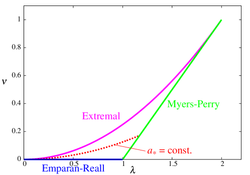
Figure 1: The parameter space $(\lambda,\nu)$ of the Pomeransky-Sen’kov solution. $\lambda$ and $\nu$ can take values in the region surrounded by solid lines. The line $\nu=\lambda-1$ is the Myers-Perry black hole limit, the line $\nu=0$ is the Emparan-Reall black ring limit, and the line $\nu=\lambda^{2}/4$ is the extremal limit. The point $\lambda=\nu=0$ corresponds to the boosted Kerr string limit. The broken line $\nu=a_{\ast}^{2}\lambda^{2}/4$ is the path to the point $\lambda=\nu=0$ with a fixed $a_{\ast}$.

The mass and angular momenta are

$$M=\frac{3\pi R^{2}\lambda}{1-\lambda+\nu},\qquad J_{\phi}=\frac{4\pi R^{3}\lambda\sqrt{\nu}\sqrt{(1+\nu)^{2}-\lambda^{2}}}{(1-\nu)^{2}(1-\lambda+\nu)},$$ (8)

$$J_{\psi}=\frac{2\pi R^{3}\lambda(1+\lambda-6\nu+\lambda\nu+\nu^{2})\sqrt{(1+\nu)^{2}-\lambda^{2}}}{(1-\nu)^{2}(1-\lambda+\nu)^{2}}.$$ (9)

The angular velocities, the area, and the surface gravity of the horizon are written as Elvang:2007hs

$$\Omega_{\phi}=\frac{\lambda(1+\nu)-(1-\nu)\sqrt{\lambda^{2}-4\nu}}{4R\lambda\sqrt{\nu}}\sqrt{\frac{1+\nu-\lambda}{1+\nu+\lambda}},\qquad\Omega_{\psi}=\frac{1}{2R}\sqrt{\frac{1+\nu-\lambda}{1+\nu+\lambda}},$$ (10)

$$A_{H}=\frac{32\pi^{2}R^{3}\lambda(1+\nu+\lambda)}{(1-\nu)^{2}(y_{h}^{-1}-y_{h})},\qquad\kappa=\frac{(y_{h}^{-1}-y_{h})(1-\nu)\sqrt{\lambda^{2}-4\nu}}{4R\lambda(1+\nu+\lambda)}.$$ (11)

II.2 Thin ring limit

We consider a thin ring limit $\lambda\to 0$ where the ratio of the $S^{2}$ radius to the $S^{1}$ radius becomes very small. Here, we have to take care of the fact that this limit depends on the path to the point $\lambda=\nu=0$. For example, taking the limit $\lambda\to 0$ on the line $\nu=0$ gives a boosted Schwarzschild string, while taking the limit $\lambda\to 0$ on the extremal line $\nu=\lambda^{2}/4$ should result in an extremal Kerr black string. Therefore, $\lambda=\nu=0$ is a degenerate point, and in order to resolve this degeneracy, we introduce a new parameter $a_{\ast}$ as

$$\nu=\frac{1}{4}a_{\ast}^{2}\lambda^{2},$$ (12)

and consider a limit $\lambda\to 0$ on the line of a fixed $a_{\ast}$ (see Fig. 1). Also, in order to obtain a well-defined limit, we introduce

$$M_{K}=\frac{1}{\sqrt{2}}\lambda R,$$ (13)

and fix $M_{K}$ in taking this limit.

We introduce the new coordinates $r$, $z$ and $\theta$ as

$$y=-\frac{\sqrt{2}R}{r},\qquad\psi=-\frac{z}{\sqrt{2}R},\qquad x=\cos\theta,$$ (14)

and collect the leading-order term of each metric component with respect to $\lambda$. Then, the black ring solution is reduced to the so-called boosted Kerr string solution

$$ds^{2}=-\left(1-\frac{2M_{K}r\cosh^{2}\sigma}{\rho^{2}}\right)dt^{2}+\frac{2M_{K}r\sinh 2\sigma}{\rho^{2}}dtdz+\left(1+\frac{2M_{K}r\sinh^{2}\sigma}{\rho^{2}}\right)dz^{2}\\ +\frac{\rho^{2}}{\Delta}dr^{2}+\rho^{2}d\theta^{2}+\frac{\left(r^{2}+a^{2}\right)^{2}-\Delta a^{2}\sin^{2}\theta}{\rho^{2}}\sin^{2}\theta d\phi^{2}\\ -\frac{4M_{K}r\cosh\sigma}{\rho^{2}}a\sin^{2}\theta dtd\phi-\frac{4M_{K}r\sinh\sigma}{\rho^{2}}a\sin^{2}\theta dzd\phi,$$ (15)

where $\rho^{2}=r^{2}+a^{2}\cos^{2}\theta$ and $\Delta=r^{2}-2M_{K}r+a^{2}$, and $a$ is defined by $a:=M_{K}a_{\ast}$. Since $M_{K}$ and $a$ correspond to the mass and rotational parameter of a four-dimensional Kerr black hole, respectively, $a_{\ast}$ represents the nondimensional rotation parameter along $S^{2}$ direction. $\sigma:=\mathrm{arctanh}(1/\sqrt{2})$ is the boost parameter. Although the boost parameter can take any value for a general boosted Kerr string, it is restricted to this value for the thin limit of a black ring. The event horizon is located at $r=r_{+}$ where $r_{\pm}:=M_{K}\pm\sqrt{M_{K}^{2}-a^{2}}=M_{K}(1\pm\sqrt{1-a_{*}^{2}})$.

In studying the evaporation of a black ring, we use this boosted Kerr string solution in the following sense. We consider the situation where $\lambda$ is very small, and do not take the exact limit. Then, in the neighborhood of the black ring, the spacetime metric can be well approximated by the boosted Kerr string solution. For this reason, the value of $R$ is not infinite in our analysis although it is very large compared to $M_{K}$. The relative error in this approximation is $O(\lambda)$ compared to the leading order in the following analyses.

In this thin-limit approximation, the physical quantities in Eqs. (8)–(11) are expressed in terms of $R,M_{K}$ and $a$ (or $a_{*}$) as

$$M\simeq 3\sqrt{2}\pi RM_{K},\qquad J_{\psi}\simeq 2\sqrt{2}\pi R^{2}M_{K},\qquad J_{\phi}\simeq 4\pi a_{\ast}RM_{K}^{2}.$$ (16)

$$\Omega_{\phi}\simeq\frac{a}{2M_{K}r_{+}}\frac{1}{\cosh\sigma},\qquad\Omega_{\psi}\simeq\frac{1}{2R},$$ (17)

$$A_{H}\simeq 16\pi^{2}r_{+}M_{K}R,\qquad\kappa\simeq\frac{r_{+}-r_{-}}{4M_{K}r_{+}}\frac{1}{\cosh\sigma}.$$ (18)

The inverse relations of Eq. (16) are

$$R\simeq\frac{3J_{\psi}}{2M},\qquad M_{K}\simeq\frac{\sqrt{2}}{9\pi}\frac{M^{2}}{J_{\psi}},\qquad a_{\ast}\simeq\frac{27\pi}{4}\frac{J_{\psi}J_{\phi}}{M^{3}},$$ (19)

and $\lambda$ is expressed as

$$\lambda=\frac{\sqrt{2}M_{K}}{R}\simeq\frac{4}{27\pi}\frac{M^{3}}{J_{\psi}^{2}}.$$ (20)

Because $\lambda^{-1/2}$ is proportional to the angular momentum $J_{\psi}$ normalized by mass $M$, it can be interpreted as the nondimensional rotation parameter along $S^{1}$. At the same time, Eq. (20) also means that $\lambda$ gives the order of the ratio of the $S^{2}$ radius to the $S^{1}$ radius. Therefore, $\lambda$ is interpreted as an indicator for the “thickness” of the black ring. In this paper, we call $\lambda$ the thickness parameter.

II.3 Effect of boost

Note that $\Omega_{\phi}$ in Eq. (17) is equal to the angular velocity defined by the Killing generator $\xi$ of the horizon of the boosted Kerr string,

$$\xi=\partial_{t}+\Omega_{\phi}\partial_{\phi}+V\partial_{z}$$ (21)

with

$$V=\tanh\sigma,$$ (22)

and $\kappa$ in Eq. (18) is identical to the surface gravity of the horizon calculated with $\xi$. For a later convenience, it is useful to compare $\Omega_{\phi}$ and $\kappa$ with the angular velocity and the surface gravity of the horizon of the unboosted Kerr string. In the following, quantities in the unboosted system are indicated by prime $(\ {}^{\prime}\ )$. In the unboosted system, the Killing generator of the horizon is $\xi^{\prime}=\partial_{t^{\prime}}+\Omega_{\phi}^{\prime}\partial_{\phi}$, and $\Omega_{\phi}^{\prime}$ and $\kappa^{\prime}$ calculated from $\xi^{\prime}$ are

$$\Omega_{\phi}^{\prime}=\frac{a}{2M_{K}r_{+}},\qquad\kappa^{\prime}=\frac{r_{+}-r_{-}}{4M_{K}r_{+}}.$$ (23)

There is a deference in the quantities of the boosted and unboosted systems by a factor of $1/\cosh\sigma$. This is understood as the effect of time delay in the Lorentz boost.

III Formulation

In this section, we formulate the time evolution of mass and angular momenta of a thin black ring via Hawking radiation, by approximating the evolution of a scalar field in the black ring spacetime by that in a boosted Kerr string spacetime.

III.1 Emission rate

The evolution of a scalar field is governed by the Klein-Gordon equation in curved spacetime

$$\left(-g\right)^{-1/2}\partial_{\mu}\left(\sqrt{-g}g^{\mu\nu}\partial_{\nu}\Phi\right)=0,$$ (24)

where $g$ is the determinant of its metric.

To quantize the field, we need to expand it in terms of the eigenmodes for $\Phi$, which can be written in the black ring background as

$$\Phi=e^{-i\omega t}e^{im\phi}e^{in\psi}\Psi(x,y),$$ (25)

where $\omega$, $m$ and $n$ are the eigenvalues for the Killing vector fields $\partial_{t}$, $\partial_{\psi}$ and $\partial_{\phi}$, respectively. By inserting this expression into Eq. (24), we obtain a second-order elliptic equation for $\Psi(x,y)$ in the $(x,y)$ plane. This equation has a discrete series of regular solutions labeled by an integer $\ell$. In the Schwarzschild string limit with $J_{\phi}=0$, this series of solutions become proportional to the associate Legendre functions $P^{m}_{\ell}(x)$. Thus, the mode functions are labeled by the four parameters $(\omega,\ell,m,n)$ in which $\ell$, $m$ and $n$ take integer values.

In the case of a nonrotating black hole, the expected number of particles emitted per unit time for each mode is proportional to black body radiation:

$$\langle N_{s}\rangle\propto\frac{1}{e^{\omega/T_{s}}-1},$$ (26)

where $\omega$ is the energy of a scalar particle in the background of the nonrotating black hole and $T_{s}$ is the temperature of the horizon. Here, the temperature is expressed as $T_{s}=\kappa_{s}/2\pi$ in terms of the surface gravity $\kappa_{s}$ of the horizon.

In the rotating case, we have to replace $\omega$ by the energy of the mode with respect to the null geodesic generator of the black hole horizons because the mode function behaves as $\exp(-i\omega_{*}u_{\pm})$ in the coordinates that are regular around the black hole horizon, where $u_{\pm}$ is the advanced time/retarded time around the horizon. In general, this null geodesic generator $\xi$ can be written as $\xi=\partial_{t}+\sum_{j}\Omega_{j}\partial_{\phi^{j}}$ in terms of the time translation Killing vector $\partial_{t}$ and the rotational Killing vectors $\partial_{\phi^{j}}$. From this, it follows that $\omega_{*}$ for the mode $\propto\exp(-i\omega t+i\sum_{j}m_{j}\phi^{j})$ is expressed as

$$\omega_{*}=\omega-\sum_{j}m^{j}\Omega_{j}.$$ (27)

Hence, the expected number of particles emitted per unit time for each mode from the black ring is given by

$$\langle N_{\rm BR}\rangle=\frac{\Gamma^{\rm(BR)}_{{\ell}mn}(\omega)}{e^{(\omega-n\Omega_{\psi}-m\Omega_{\phi})/T_{\rm BR}}-1},$$ (28)

where $T_{\rm BR}$ is the temperature of the horizon and $\Gamma^{\rm(BR)}_{{\ell}mn}(\omega)$ is the greybody factor, which is identical to the absorption probability of the incoming wave of the corresponding modes. This determines the emission rates of the total mass $M$ and angular momenta $J_{\psi}$ and $J_{\phi}$ as

$$-\frac{d}{dt}\left(\begin{array}[]{ccc}M\\ J_{\psi}\\ J_{\phi}\\ \end{array}\right)=\frac{1}{2\pi}\sum_{\ell,m,n}\int^{\infty}_{0}d\omega\langle N_{\rm BR}\rangle\left(\begin{array}[]{ccc}\omega\\ n\\ m\\ \end{array}\right),$$ (29)

where the summation is taken over all modes. Note that in this expression, it is difficult to estimate the greybody factor generally because we cannot separate the coordinates $x$ and $y$, and two-dimensional numerical calculations are required to determine the energy eigenvalues and corresponding eigenmodes.

In order to circumvent this difficulty, we consider the situation where the mode functions can be approximately evaluated: a black string limit discussed above. For the boosted black string (15), we can separate the wave equation, and therefore, we approximate the evolution of a scalar field in a black ring spacetime by that in a boosted Kerr string spacetime. In this situation, the variables can be separated as

$$\Phi=e^{-i\omega t}R(r)e^{-ikz}e^{im\phi}S^{m}_{\ell}(\theta),$$ (30)

where $S^{m}_{\ell}(\theta)$ is the spheroidal harmonic function. From the coordinate transformation (14), $n$ of a black ring and $k$ of a boosted black string are related by

$$n=2kR\tanh\sigma.$$ (31)

The expected number of particles emitted per unit time per mode is given by

$$\langle N_{\rm BBS}\rangle=\frac{\Gamma_{\ell mn}(\omega)}{e^{(\omega-kV-m\Omega_{\phi})/T}-1},$$ (32)

where $T=\kappa/2\pi$ is the temperature of the horizon with $\kappa$ in Eq. (18), and $V$ is the linear velocity introduced in Eq. (22). $\Gamma_{\ell mn}(\omega)$ is the greybody factor of the boosted Kerr string spacetime. We evaluate the emission rates (29) by using $\langle N_{\rm BBS}\rangle$ instead of $\langle N_{\rm BR}\rangle$.

III.2 Simplification

We normalize all quantities by the mass density $M_{K}$,

$$\tilde{\omega}=M_{K}\omega,\qquad\tilde{k}=M_{K}k,\qquad\tilde{\Omega}_{\phi}=M_{K}\Omega_{\phi},\qquad\tilde{T}=M_{K}T=\frac{M_{K}\kappa}{2\pi}.$$ (33)

We change the order of summations over $\ell$ and $m$ as

$$\sum_{\ell=0}^{\infty}\sum_{m=-\ell}^{\ell}=\sum_{m=-\infty}^{\infty}\sum_{\ell=|m|}^{\infty},$$ (34)

and introduce

$$g^{(m)}(\tilde{\omega},\tilde{k}):=\sum_{\ell=|m|}^{\infty}\Gamma_{\ell mn}(\tilde{\omega}),$$ (35)

where $\tilde{k}$ and $n$ are related to each other by Eq. (31). Then, the emission rates can be written as

$$-\frac{d}{dt}\left(\begin{array}[]{ccc}M\\ J_{\psi}\\ J_{\phi}\\ \end{array}\right)=\frac{1}{2\pi M_{K}}\sum_{m=-\infty}^{\infty}\sum_{n=-\infty}^{\infty}\int^{\infty}_{|\tilde{k}|}d\tilde{\omega}\frac{g^{(m)}(\tilde{\omega},\tilde{k})}{e^{(\tilde{\omega}-\tilde{k}V-m\tilde{\Omega}_{\phi})/\tilde{T}}-1}\left(\begin{array}[]{ccc}\tilde{\omega}/M_{K}\\ n\\ m\\ \end{array}\right).$$ (36)

Here, the lower limit of the integral is $|\tilde{k}|$ because the modes with their energy $\omega<|\tilde{k}|$ are gravitationally bounded and do not escape to infinity. Because the spectral density of $\tilde{k}$ is very large, $O(1/\lambda)$, the summation over $n$ can be replaced by the integral:

$$\sum_{n}\to\int dn=\frac{2R\tanh\sigma}{M_{K}}\int d\tilde{k}.$$ (37)

The relative error produced by this replacement is $O(\lambda)$ and negligible in our thin-limit approximation. We obtain

$$-\frac{dM}{dt}=\frac{R}{\sqrt{2}\pi M_{K}^{3}}\sum_{m=-\infty}^{\infty}\int_{-\infty}^{\infty}d\tilde{k}\int_{|\tilde{k}|}^{\infty}d\tilde{\omega}\frac{\tilde{\omega}g^{(m)}(\tilde{\omega},\tilde{k})}{e^{(\tilde{\omega}-\tilde{k}V-m\tilde{\Omega}_{\phi})/\tilde{T}}-1},$$ (38)

$$-\frac{dJ_{\psi}}{dt}=\frac{R^{2}}{\pi M_{K}^{3}}\sum_{m=-\infty}^{\infty}\int_{-\infty}^{\infty}d\tilde{k}\int_{|\tilde{k}|}^{\infty}d\tilde{\omega}\frac{\tilde{k}g^{(m)}(\tilde{\omega},\tilde{k})}{e^{(\tilde{\omega}-\tilde{k}V-m\tilde{\Omega}_{\phi})/\tilde{T}}-1}.$$ (39)

$$-\frac{dJ_{\phi}}{dt}=\frac{R}{\sqrt{2}\pi M_{K}^{2}}\sum_{m=-\infty}^{\infty}\int_{-\infty}^{\infty}d\tilde{k}\int_{|\tilde{k}|}^{\infty}d\tilde{\omega}\frac{mg^{(m)}(\tilde{\omega},\tilde{k})}{e^{(\tilde{\omega}-\tilde{k}V-m\tilde{\Omega}_{\phi})/\tilde{T}}-1}.$$ (40)

The integral in each formula can be further simplified if we perform the transformation from $(\tilde{\omega},\tilde{k})$ to $(\tilde{\omega}^{\prime},\tilde{k}^{\prime})$,

$$\tilde{\omega}=\tilde{\omega}^{\prime}\cosh\sigma+\tilde{k}^{\prime}\sinh\sigma,\qquad\tilde{k}=\tilde{\omega}^{\prime}\sinh\sigma+\tilde{k}^{\prime}\cosh\sigma.$$ (41)

Substituting these formulas with $\cosh\sigma=\sqrt{2}$ and $\sinh\sigma=1$ and rewriting $M_{K}$ and $R$ by $M$, $J_{\psi}$ and $J_{\phi}$ using Eq. (19), we obtain the simplified expression of the evolution:

$$-\frac{1}{M}\frac{dM}{dt}=2F(a_{\ast})\frac{J_{\psi}^{4}}{M^{8}},$$ (42)

$$-\frac{1}{J_{\psi}}\frac{dJ_{\psi}}{dt}=3F(a_{\ast})\frac{J_{\psi}^{4}}{M^{8}},$$ (43)

$$-\frac{1}{J_{\phi}}\frac{dJ_{\phi}}{dt}=G(a_{\ast})\frac{J_{\psi}^{3}}{J_{\phi}M^{5}},$$ (44)

with

$$F(a_{\ast}):=\frac{3^{7}\pi^{2}}{2^{3}\sqrt{2}}\sum_{m=-\infty}^{\infty}I_{1}^{(m)}(a_{\ast}),$$ (45)

$$G(a_{\ast}):=\frac{3^{5}\pi}{2^{2}\sqrt{2}}\sum_{m=-\infty}^{\infty}I_{2}^{(m)}(a_{\ast}).$$ (46)

Here, we defined

$$I_{1}^{(m)}(a_{\ast}):=\int^{\infty}_{-\infty}d\tilde{k}^{\prime}\int^{\infty}_{|\tilde{k}^{\prime}|}d\tilde{\omega}^{\prime}\frac{\tilde{\omega}^{\prime}g^{\prime(m)}(\tilde{\omega}^{\prime},\tilde{k}^{\prime})}{e^{(\tilde{\omega}^{\prime}-m\tilde{\Omega}^{\prime}_{\phi})/\tilde{T}^{\prime}}-1},$$ (47)

$$I_{2}^{(m)}(a_{\ast}):=\int^{\infty}_{-\infty}d\tilde{k}^{\prime}\int^{\infty}_{|\tilde{k}^{\prime}|}d\tilde{\omega}^{\prime}\frac{mg^{\prime(m)}(\tilde{\omega}^{\prime},\tilde{k}^{\prime})}{e^{(\tilde{\omega}^{\prime}-m\tilde{\Omega}^{\prime}_{\phi})/\tilde{T}^{\prime}}-1},$$ (48)

with $g^{\prime(m)}(\tilde{\omega}^{\prime},\tilde{k}^{\prime})=g^{(m)}(\tilde{\omega},\tilde{k})$. In the same manner as Eq. (33), we normalized the quantities ${\Omega}_{\phi}^{\prime}$ and ${T}^{\prime}=\kappa^{\prime}/2\pi$ of the unboosted system in Eq. (23) as $\tilde{\Omega}_{\phi}^{\prime}:=M_{K}\Omega_{\phi}^{\prime}$ and $\tilde{T}^{\prime}:=M_{K}T^{\prime}$. Their explicit formulas are

$$\tilde{\Omega}_{\phi}^{\prime}=\frac{(1/2)a_{*}}{1+\sqrt{1-a_{*}^{2}}},\qquad\tilde{T}^{\prime}=\frac{(1/4\pi)\sqrt{1-a_{*}^{2}}}{1+\sqrt{1-a_{*}^{2}}},$$ (49)

and depend only on $a_{*}$. Note that we used the fact that the integrals of terms proportional to $\tilde{k}^{\prime}$ vanish because the greybody factor is an even function of $\tilde{k}^{\prime}$ (see Eqs. (55) and (56) of the next subsection), and thus, such terms are odd functions of $\tilde{k}^{\prime}$. From Eqs. (42)–(44) and Eq. (19), the equation for $a_{\ast}$ is derived as

$$-\frac{1}{a_{\ast}}\frac{da_{\ast}}{dt}=3H(a_{\ast})\frac{J_{\psi}^{4}}{M^{8}},$$ (50)

where

$$H(a_{\ast}):=\frac{9\pi}{4}\frac{G(a_{\ast})}{a_{\ast}}-F(a_{\ast}).$$ (51)

Therefore, the time evolution of a thin black ring by the Hawking radiation is determined by the equations for $M$, $J_{\psi}$ and $a_{\ast}$, that is, Eqs. (42), (43) and (50). The remaining task is to calculate the greybody factors and obtain $F(a_{\ast})$ and $H(a_{\ast})$ of Eqs. (45) and (51) numerically.

III.3 Greybody factor

In the following, we discuss the greybody factor for a massless scalar field in a boosted Kerr string spacetime. Substituting the ansatz (30) into the Klein-Gordon equation (24) in the background of the boosted Kerr string (15), we get the following angular and radial wave equations for $S^{m}_{\ell}(\theta)$ and $R(r)$ Dias:2006zv :

$$0=\frac{1}{\sin\theta}\partial_{\theta}\left(\sin\theta\partial_{\theta}S^{m}_{\ell}\right)+\left[a^{2}\left(\omega^{2}-k^{2}\right)\cos^{2}\theta-\frac{m^{2}}{\sin^{2}\theta}+\lambda_{\ell m}\right]S^{m}_{\ell},$$ (52)

$$0=\Delta\partial_{r}\left(\Delta\partial_{r}R\right)-\Delta\left[k^{2}r^{2}+a^{2}\omega^{2}-2\omega ma\cosh\sigma+\lambda_{\ell m}\right]R\\ +\Big{[}\left[\omega\left(r^{2}+a^{2}\right)-ma\cosh\sigma\right]^{2}+2M_{K}r\left(r^{2}+a^{2}\right)\cosh^{2}\sigma\left(\omega-k\tanh\sigma\right)^{2}\\ -2M_{K}r\left(r^{2}+a^{2}\right)\omega^{2}-m^{2}a^{2}\sinh^{2}\sigma+4kmaM_{K}r\sinh\sigma\Big{]}R,$$ (53)

where $\lambda_{\ell m}$ is the separation constant which is determined as an eigenvalue of (52). For small $a^{2}\left(\omega^{2}-k^{2}\right)$, the eigenvalues associated with the spheroidal wave functions $S^{m}_{\ell}$ are $\lambda_{\ell m}=\ell\left(\ell+1\right)+{\cal O}\left(a^{2}\left(\omega^{2}-k^{2}\right)\right)$ Teukolsky:1973ha .

As we mentioned in Sec. III.1, the greybody factor is calculated as the absorption probability of the incoming waves of the corresponding mode. With the tortoise coordinate $r_{\ast}$ and the new wave function $u$ defined by

$$dr_{\ast}=\frac{r^{2}+a^{2}}{\Delta}dr,\qquad R=\frac{1}{\sqrt{r^{2}+a^{2}}}u,$$ (54)

the radial wave equation (53) can be rewritten as the following equation of Schrödinger type:

$$\left[\frac{d^{2}}{dr_{\ast}^{2}}+{\omega^{\prime}}^{2}-V(r)\right]u=0,$$ (55)

where $V(r)$ is the effective potential

$$V(r)=\frac{\Delta\left\{2M_{K}r(r^{2}-2a^{2})+a^{2}(r^{2}+a^{2})\right\}}{(r^{2}+a^{2})^{4}}+\frac{\Delta({\omega^{\prime}}^{2}a^{2}+\lambda_{\ell m}+{k^{\prime}}^{2}r^{2})+4m\omega^{\prime}M_{K}ar-m^{2}a^{2}}{(r^{2}+a^{2})^{2}}.$$ (56)

Here, the quantities in the unboosted frame, $\omega^{\prime}$ and $k^{\prime}$, were introduced in the same manner as Eq. (41). Note that Eqs. (55) and (56) have the same form as the equations for a massive scalar field with angular frequency $\omega^{\prime}$ and mass $|k^{\prime}|$ in a four-dimensional Kerr spacetime. As the boundary condition, we impose the ingoing condition at the horizon. Then, $u$ behaves as

$$u(r_{\ast})\sim\begin{cases}&e^{-i\omega_{+}^{\prime}r_{\ast}}\hskip 113.81102pt\text{at}\qquad r\to r_{+},\\ &A_{in}e^{-i\omega_{\infty}^{\prime}r_{\ast}}+A_{out}e^{i\omega_{\infty}^{\prime}r_{\ast}}\hskip 28.45274pt\text{at}\qquad r\to\infty.\end{cases}$$ (57)

Here $\omega_{+}^{\prime}:=\omega^{\prime}-m\Omega_{\phi}^{\prime}$ and $\omega_{\infty}^{\prime}:=\sqrt{{\omega^{\prime}}^{2}-{k^{\prime}}^{2}}$. The greybody factor is written as

$$\Gamma^{\prime}_{\ell m}(\omega^{\prime},k^{\prime})=1-\left|\frac{A_{out}}{A_{in}}\right|^{2},$$ (58)

which has to be evaluated numerically.

In this paper, we perform numerical calculations of the greybody factor in the case of the Emparan-Reall black ring, i.e., $a=0$. In this case, $S^{m}_{\ell}(\theta)e^{im\phi}$ becomes the spherical harmonic function $Y_{\ell m}(\theta,\phi)$ and the greybody factor is independent of $m$, and therefore, the calculation becomes much simpler compared to the case $a\neq 0$. We developed a code to calculate the greybody factor in this situation. The left and right panels of Fig. 2 show the behaviors of the greybody factors of the first three even $\ell$ numbers for $\tilde{k}^{\prime}=0$ and $0.6$, respectively. Our result is in good agreement with the analytic approximate formula for low-frequency waves in Ref. Unruh:1976fm (see also Jung:2004nh ; Kanti:2010mk ).

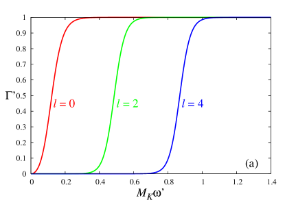
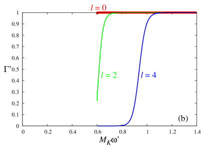
Figure 2: Greybody factors $\Gamma^{\prime}$ as functions of $M_{K}\omega^{\prime}$ for the modes $\ell=0$, $2$, and $4$ in the case $a_{*}=0$ for (a) $M_{K}k^{\prime}=0$ (left panel) and (b) $M_{K}k^{\prime}=0.6$ (right panel). In the right panel, the data for $M_{K}\omega^{\prime}\geq 0.6005$ are plotted.

Note that if we take the limit $\tilde{\omega}^{\prime}\to\tilde{k}^{\prime}$ for $\tilde{k}^{\prime}\neq 0$, the greybody factor is expected to approach a nonzero finite value. Obtaining these values by numerical calculation is rather difficult because the greybody factors have to be evaluated at a very distant position $r/M\gg 1/v^{\prime 2}$ with $v^{\prime}=\sqrt{1-(k^{\prime}/\omega^{\prime})^{2}}$. Although these values are left uncertain in our calculation, we have checked that the error caused by this uncertainty is small. For example, the error in $F(0)$ of Eq. (67) is smaller than 0.1%.

IV Evolution by Evaporation

In this section, we discuss general features of the time evolution of the evaporating Pomeransky-Sen’kov black ring. Then, we focus attention to the case of the Emparan-Reall black ring, and derive semi-analytic solutions of the time evolution using the numerical results of the greybody factors.

IV.1 Evolution of Pomeransky-Sen’kov black rings

First, we discuss general features that does not depend on the details of the greybody factor. From Eqs. (42) and (43), the following relation can be immediately found:

$$\frac{J_{\psi}^{2}}{M^{3}}=\text{const.}$$ (59)

From Eq. (20), this means that the thickness parameter $\lambda$ does not change,

$$\lambda(t)\equiv\lambda(0).$$ (60)

Therefore, a Pomeransky-Sen’kov black ring evaporates without changing the initial value of the nondimensional rotation parameter along $S^{1}$.

Next, let us assume $a_{*}>0$ and consider how to solve the evolution equations for $a_{*}(t)$ and $M(t)$. Eliminating $M$ and $J_{\psi}$ from Eqs. (42) and (50) using Eq. (59), we obtain

$$\frac{d}{dt}\left(\frac{3a_{*}H(a_{*})}{da_{*}/dt}\right)=4F(a_{*}).$$ (61)

In principle, this equation can be solved at least numerically to yield $a_{\ast}(t)$ once $H(a_{*})$ and $F(a_{*})$ are specified. Then, from Eqs. (42) and (50), the time evolution of $M(t)$ is formally given by

$$M(t)=M(0)\exp\left[\frac{2}{3}\int_{a_{\ast}(0)}^{a_{\ast}(t)}\frac{F(a_{\ast})}{a_{\ast}H(a_{\ast})}da_{\ast}\right].$$ (62)

We point out that the behavior of $H(a_{*})$ is crucial for the evolution of $a_{*}$. This function is analogous to $h(a_{*})$ of Ref. Chambers:1997ai where evolution of a four-dimensional Kerr black hole was investigated: The value of $a_{*}$ increases (decreases) if $H(a_{*})$ is negative (positive). If $H(a_{*})$ crosses zero from negative to positive at some value $a_{*}=a_{*}^{(c)}$ similarly to Fig. 3 of Ref. Chambers:1997ai , the black ring inevitably evolves to the state with $a_{*}^{(c)}$. Therefore, numerical calculation of $H(a_{*})$ is very interesting, but is left for future work. In the present paper, we only study what happens in the case of an Emparan-Reall black ring.

IV.2 Evolution of Emparan-Reall black rings

In the case of the Emparan-Reall black ring, $J_{\phi}(t)\equiv 0$ and $a_{\ast}\equiv 0$, and Eqs. (42) and (43) can be solved analytically:

$$M(t)=M(0)\left(1-4F(0)\frac{J_{\psi}(0)^{4}}{M(0)^{8}}t\right)^{1/2},$$ (63)

$$J_{\psi}(t)=J_{\psi}(0)\left(1-4F(0)\frac{J_{\psi}(0)^{4}}{M(0)^{8}}t\right)^{3/4}.$$ (64)

Therefore, our remaining task is to determine $F(0)$ numerically.

As discussed in Sec. III.2, basically we have to calculate Eqs. (35), (47), and (45), and in those equations, the summation over $m$ was taken at the last step. But in the case of $a_{*}=0$ considered here, it is better to take the summation with respect to $m$ in advance because the integrand does not depend on $m$. For this reason, we calculate summation of the greybody factors as

$$g^{\prime}(\tilde{\omega}^{\prime},\tilde{k}^{\prime}):=\sum_{\ell=0}^{\infty}\sum_{m=-\ell}^{\ell}\Gamma^{\prime}_{\ell m}(\tilde{\omega}^{\prime},\tilde{k}^{\prime})=\sum_{\ell=0}^{\infty}(2\ell+1)\Gamma^{\prime}_{\ell}(\tilde{\omega}^{\prime},\tilde{k}^{\prime}).$$ (65)

Then, $F(0)$ is given by

$$F(0)=\frac{3^{7}\pi^{2}}{2^{3}\sqrt{2}}I_{1},\qquad I_{1}:=\int_{-\infty}^{\infty}d\tilde{k}^{\prime}\int_{|\tilde{k}^{\prime}|}^{\infty}d\tilde{\omega}^{\prime}\frac{\tilde{\omega}^{\prime}g^{\prime}(\tilde{\omega}^{\prime},\tilde{k}^{\prime})}{e^{\tilde{\omega}^{\prime}/\tilde{T}^{\prime}}-1}.$$ (66)

The integrations of $I_{1}$ were executed with the Simpson’s method. The domain of integration of $I_{1}$ was made finite by discarding the region where the integrand is sufficiently small. We therefore set the upper limit of integration with respect to $\tilde{\omega}^{\prime}$ to be $0.75$. We took summation with respect to $\ell$ up to $\ell=5$, because the contributions from the modes $\ell>5$ turned out to be negligible. This is because the potential walls for $\ell>5$ are so high that they reflect almost of all waves. In this manner, $F(0)$ is determined as

$$F(0)\simeq 0.239.$$ (67)

As a check, we compute $F(0)$ using the DeWitt approximation DeWitt:1975 in Appendix A. The two results agree well, and therefore, our numerical result is reliable.

As shown in Eq. (60), the nondimensional rotation parameter $J_{\psi}^{2}/M^{3}$ is held fixed throughout the evolution, and this also indicates the constancy of the thickness parameter $\lambda$. Because $a_{*}\equiv 0$, the Emparan-Reall black ring evaporates keeping similarity to its initial shape: The black ring at any time can be obtained by uniformly scaling its initial configuration. The scaling factor $C(t)$ can be found by deriving the time evolution of the ring radius $R$ as

$$C(t):=\frac{R(t)}{R(0)}=\left(1-4F(0)\frac{J_{\psi}(0)^{4}}{M(0)^{8}}t\right)^{1/4}.$$ (68)

The lifetime $t_{\rm LT}$ of a thin black ring with mass $M$ is

$$t_{\rm LT}\approx\left(\frac{27\pi\lambda}{4}\right)^{2}\left(\frac{M}{M_{p}}\right)^{2}t_{p},$$ (69)

where $M_{p}$ and $t_{p}$ are the Planck mass $(\hbar^{2}/G)^{1/3}$ and the Planck time $\hbar/M_{p}c^{2}$, respectively. The time scale is proportional to $M^{2}$, and this dependence on $M$ is same as that of the five-dimensional Schwarzschild black hole. However, because of the prefactor $(27\pi\lambda/4)^{2}$, the lifetime of a thin black ring with $\lambda\lesssim 10^{-2}$ is much shorter than that of the five-dimensional Schwarzschild black hole with the same mass.

V Energy and angular spectra

In this section, we study the spectra of energy and angular momentum of radiated particles in the evaporation of a thin Emparan-Reall black ring.

V.1 Formulas for energy and angular spectra

For a thin Emparan-Reall black ring with $a_{\ast}=0$, the emission rates of energy and angular momentum are given by Eqs. (38) and (39) with $dJ_{\phi}/dt=0$. In Sec. III.2, we simplified these formulas by performing the Lorentz transformation from $(\tilde{\omega},\tilde{k})$ to $(\tilde{\omega}^{\prime},\tilde{k}^{\prime})$ through Eq. (41). Physically, this corresponds to the transformation from the boosted frame to the unboosted frame. Therefore, when we speak about the spectra, the two kinds of spectra can be considered: The spectra in the boosted frame (with respect to $\omega$) and those in the unboosted frame (with respect to $\omega^{\prime}$). In this paper, we prefer to analyze the spectra in the boosted frame, because the spectra in the boosted frame correspond to those for a distant observer at rest in the original black ring spacetime. For this reason, we rewrite Eqs. (38) and (39) in order to match them to our purpose here. Because the integrand does not depend on $m$ in the case of $a_{\ast}=0$, we take summation with respect to $m$ in advance,

$$\sum_{m=-\infty}^{\infty}g^{(m)}(\tilde{\omega},\tilde{k})=\sum_{\ell=0}^{\infty}\left(2\ell+1\right)\Gamma_{\ell}(\tilde{\omega},\tilde{k}),$$ (70)

and change the order of integration with respect to $\tilde{\omega}$ and $\tilde{k}$ as

$$\int_{-\infty}^{\infty}d\tilde{k}\int_{|\tilde{k}|}^{\infty}d\tilde{\omega}=\int_{0}^{\infty}d\tilde{\omega}\int_{-\tilde{\omega}}^{\tilde{\omega}}d\tilde{k}.$$ (71)

Then, the formulas for the emission rates become

$$-\frac{dM}{dt}=\frac{R}{\sqrt{2}\pi M_{K}^{3}}\int_{0}^{\infty}d\tilde{\omega}\sum_{\ell=0}^{\infty}\left(2\ell+1\right)\int_{-\tilde{\omega}}^{\tilde{\omega}}d\tilde{k}\frac{\tilde{\omega}\Gamma_{\ell}(\tilde{\omega},\tilde{k})}{e^{(\tilde{\omega}-\tilde{k}V)/\tilde{T}}-1},$$ (72)

$$-\frac{dJ_{\psi}}{dt}=\frac{R^{2}}{\pi M_{K}^{3}}\int_{0}^{\infty}d\tilde{\omega}\sum_{\ell=0}^{\infty}\left(2\ell+1\right)\int_{-\tilde{\omega}}^{\tilde{\omega}}d\tilde{k}\frac{\tilde{k}\Gamma_{\ell}(\tilde{\omega},\tilde{k})}{e^{(\tilde{\omega}-\tilde{k}V)/\tilde{T}}-1}.$$ (73)

Therefore, the energy and angular spectra are written as

$$-\frac{d^{2}M}{dtd\tilde{\omega}}=\frac{R}{\sqrt{2}\pi M_{K}^{3}}\frac{dI_{M}}{d\tilde{\omega}},\qquad-\frac{d^{2}J_{\psi}}{dtd\tilde{\omega}}=\frac{R^{2}}{\pi M_{K}^{3}}\frac{dI_{J}}{d\tilde{\omega}},$$ (74)

with the definitions

$$\frac{dI_{M}}{d\tilde{\omega}}:=\sum_{\ell=0}^{\infty}\left(2\ell+1\right)\int_{-\tilde{\omega}}^{\tilde{\omega}}d\tilde{k}\frac{\tilde{\omega}\Gamma_{\ell}(\tilde{\omega},\tilde{k})}{e^{(\tilde{\omega}-\tilde{k}V)/\tilde{T}}-1},$$ (75)

$$\frac{dI_{J}}{d\tilde{\omega}}:=\sum_{\ell=0}^{\infty}\left(2\ell+1\right)\int_{-\tilde{\omega}}^{\tilde{\omega}}d\tilde{k}\frac{\tilde{k}\Gamma_{\ell}(\tilde{\omega},\tilde{k})}{e^{(\tilde{\omega}-\tilde{k}V)/\tilde{T}}-1}.$$ (76)

The quantities $dI_{M}/d\tilde{\omega}$ and $dI_{J}/d\tilde{\omega}$ are interpreted as the rescaled energy and angular spectra.

We also would like to compare the energy spectrum of a thin black ring with that of a four-dimensional Schwarzschild black hole. The energy spectrum of evaporation of a four-dimensional Schwarzschild black hole with a mass $M_{S}=M_{K}/G_{4}$, where $G_{4}$ is the four-dimensional gravitational constant, is given by

$$-\frac{d^{2}M_{S}}{dtd\tilde{\omega}}=\frac{1}{M_{K}^{2}}\frac{dI^{\rm(BH)}_{M}}{d\tilde{\omega}}\quad\textrm{with}\quad\frac{dI^{\rm(BH)}_{M}}{d\tilde{\omega}}:=\frac{1}{2\pi}\sum_{\ell=0}^{\infty}\left(2\ell+1\right)\frac{\tilde{\omega}\Gamma^{\rm(BH)}_{\ell}(\tilde{\omega})}{e^{\tilde{\omega}/\tilde{T}^{\prime}}-1},$$ (77)

where $\Gamma^{\rm(BH)}_{\ell}(\tilde{\omega})$ is the greybody factor for a massless scalar field in a four-dimensional Schwarzschild spacetime. Here, $dI_{M}^{\rm(BH)}/d\tilde{\omega}$ is the rescaled energy spectrum. The trivial difference between the two energy emission rates (72) and (77) is that the black ring evaporation is different by a factor of $\sim R/M_{K}\sim 1/\lambda\gg 1$ compared to the four-dimensional black hole evaporation. This is because a large number of the Kaluza-Klein modes contribute to the black ring evaporation, while only massless modes contribute to the evaporation of a four-dimensional Schwarzschild black hole. In the following, we discuss the difference between the rescaled energy spectra $dI_{M}/d\tilde{\omega}$ and $dI_{M}^{\rm(BH)}/d\tilde{\omega}$ apart from this trivial difference of $O(R/M_{K})$.

V.2 Numerical results

Now, we present the numerical results.

V.2.1 Energy spectrum

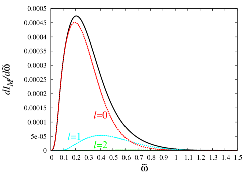
Figure 3: The rescaled energy spectrum $dI_{M}/d\tilde{\omega}$ as a function of $\tilde{\omega}$ together with the contributions of different quantum numbers $\ell=0,1$, and $2$. This profile is proportional to the energy spectrum.

Figure 3 shows the rescaled energy spectrum $dI_{M}/d\tilde{\omega}$ of emitted particles from a thin Emparan-Reall black ring as a function of $\tilde{\omega}$. The contributions from different quantum numbers $\ell=0$, $1$, and $2$ are also plotted. Only the $\ell=0$ and $1$ modes give the dominant contributions for the energy spectrum. The data for the higher multipole modes $\ell\geq 3$ are not plotted because they are tiny and invisible.

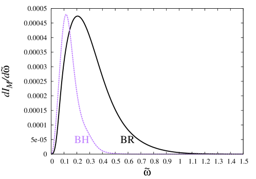
Figure 4: The rescaled energy spectra $dI_{M}/d\tilde{\omega}$ for a thin black ring and $dI^{\rm(BH)}_{M}/d\tilde{\omega}$ for a four-dimensional Schwarzschild black hole as a function of $\tilde{\omega}$.

Let us discuss the feature of the energy spectrum of the black ring evaporation by comparing it with that of the evaporation of a four-dimensional Schwarzschild black hole. The numerical data of the energy spectra for a black ring and for a four-dimensional black hole are plotted in Fig. 4. First, we focus attention to the low-frequency region, $\tilde{\omega}\ll 1$. In this region, the energy spectrum for the black ring evaporation grows more slowly compared to that for the four-dimensional black hole as $\tilde{\omega}$ is increased. This feature can be explained by the approximate analysis as follows. In this region, the energy spectrum is approximately determined only by the $\ell=0$ mode. Since the field equation in the unboosted frame is identical to the Klein-Gordon equation with mass $k^{\prime}$, we can use Unruh’s approximate formula Unruh:1976fm for the greybody factor,

$$\Gamma_{0} \approx \frac{32\pi(1+v^{\prime 2})\tilde{\omega}^{\prime 3}}{1-\exp[-2\pi\tilde{\omega}^{\prime}(1+v^{\prime 2})/v^{\prime}]}$$ (78)

$$\approx 16\tilde{\omega}^{\prime}\sqrt{\tilde{\omega}^{\prime 2}-\tilde{k}^{\prime 2}}+16\pi\tilde{\omega}^{\prime}\left(2\tilde{\omega}^{\prime 2}-\tilde{k}^{\prime 2}\right)+\cdots,$$

for the $\ell=0$ mode, where $v^{\prime}:=\sqrt{1-\tilde{k}^{\prime 2}/\tilde{\omega}^{\prime 2}}$ is the velocity at infinity. Transforming this formula into the boosted frame and substituting it into Eq. (75), we find

$$\frac{dI_{M}}{d\tilde{\omega}}\approx\tilde{\omega}^{3}.$$ (79)

On the other hand, the approximate behavior of ${dI_{M}^{\rm(BH)}}/{d\tilde{\omega}}$ for $\tilde{\omega}\ll 1$ for the four-dimensional Schwarzschild black hole is derived as

$$\frac{dI_{M}^{\rm(BH)}}{d\tilde{\omega}}\approx\pi^{-2}\tilde{\omega}^{2}.$$ (80)

This explains the slower growth of the rescaled energy spectrum for the black ring compared to that for the four-dimensional black hole.

Next, we discuss the behavior in the high-frequency region $\tilde{\omega}\gg 1$. In this case, the greybody factor for a sufficiently small $\ell$ is approximately unity (see Fig. 2 and also Eq. (96) in Appendix A), and therefore, the contribution from a mode with a sufficiently small $\ell$ is approximated as

$$\int_{-\tilde{\omega}}^{\tilde{\omega}}d\tilde{k}\frac{\tilde{\omega}\Gamma_{\ell}(\tilde{\omega},\tilde{k})}{e^{(\tilde{\omega}-\tilde{k}V)/\tilde{T}}-1}\approx\frac{\tilde{\omega}}{8\pi}{e^{-8(\sqrt{2}-1)\pi\tilde{\omega}}}.$$ (81)

Since the number of the modes that contribute to the energy spectrum is $O(\tilde{\omega}^{2})$, we have

$$\frac{dI_{M}}{d\tilde{\omega}}\sim{\tilde{\omega}^{3}}{e^{-8(\sqrt{2}-1)\pi\tilde{\omega}}}$$ (82)

for $\tilde{\omega}\gg 1$ as an order estimate. On the other hand, for a four-dimensional Schwarzschild black hole, we have

$$\frac{dI_{M}^{\rm(BH)}}{d\tilde{\omega}}\sim{\tilde{\omega}^{2}}{e^{-8\pi\tilde{\omega}}}.$$ (83)

The remarkable difference of the black ring formula (82) from the black hole formula (83) is the presence of the factor $\sqrt{2}-1\approx 0.414$ in the argument of the exponential function. Because of this factor, the energy spectrum for the black ring evaporation decays much more slowly than that for the black hole as $\tilde{\omega}$ is increased. We can also confirm this slower decay from our numerical data as shown in Fig. 4. The origin of this factor is the argument $(\tilde{\omega}-\tilde{k}V)/\tilde{T}$ in the exponential function of the denominator in the left-hand side of Eq. (81). In this formula, the momentum $\tilde{k}$ in the $z$ direction of the boosted black string spacetime enters like a chemical potential, and this “chemical potential term” enhances the emission rate of particles with positive momenta $\tilde{k}>0$. From the viewpoint of the original black ring spacetime, more number of particles with positive angular momenta are emitted. Note that similar phenomena are observed in the evaporation of Kerr and Myers-Perry black holes Kanti:2010mk ; Ida:2005 ; Harris:2005 ; Duffy:2005 ; Casals:2008 : The energy emission rate of a rotating black hole is also enhanced in the high-frequency regime compared to that of a Schwarzschild(-Tangherlini) black hole because of the effect of the chemical potential term.

The location of the peak has to be evaluated numerically. Our numerical result shows that the peak position is $\tilde{\omega}\simeq 0.21$ with the peak value $dI_{M}/d\tilde{\omega}=4.73\times 10^{-4}$. On the other hand, the peak position for the energy spectrum $dI_{M}/d\tilde{\omega}$ for a four-dimensional Schwarzschild black hole is $\tilde{\omega}\simeq 0.12$. The peak of $dI_{M}/d\tilde{\omega}$ is located at a higher frequency (in the unit of $M_{K}$) compared to that of $dI^{\rm(BH)}_{M}/d\tilde{\omega}$. The difference in the peak positions comes from both the contribution from the Kaluza-Klein modes and the effect of the chemical potential term.

To summarize, the energy spectrum of emitted particles from a black ring shifts towards higher frequency domain compared to that from a four-dimensional black hole with the same value of $M_{K}$.

V.2.2 Angular spectrum

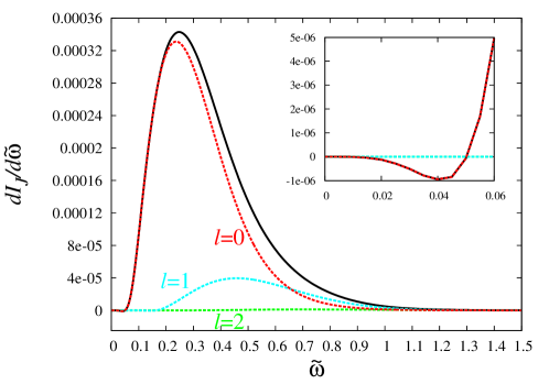
Figure 5: The rescaled angular spectrum $dI_{J}/d\tilde{\omega}$ as a function of $\tilde{\omega}$ together with the contributions of different quantum numbers $\ell=0,1$, and $2$. The inset highlights the region $0\leq\tilde{\omega}\leq 0.06$. This profile is proportional to the angular spectrum.

Now, we turn our attention to the angular spectrum. Figure 5 shows the rescaled angular spectrum $dI_{J}/d\tilde{\omega}$ as a function of $\tilde{\omega}$ together with the contributions of different quantum numbers $\ell=0,1$, and $2$. The modes $\ell\geq 3$ are not plotted for the same reason as the rescaled energy spectrum. Again, the $\ell=0$ and $1$ modes give the dominant contributions to the angular spectrum.

First, we discuss the behavior in the low-frequency region. In this region, the spectrum is approximately determined only by the $\ell=0$ mode. As we can see in the inset of Fig. 5, the rescaled angular spectrum is negative for $\tilde{\omega}\lesssim 0.05$. This behavior can be confirmed also from the approximate analysis. Substituting Unruh’s approximate formula (78) for the greybody factor of the $\ell=0$ mode into Eq. (76), we have

$$\frac{dI_{J}}{d\tilde{\omega}}\approx\left(\pi-\frac{8\sqrt{2}}{3}\right)\tilde{\omega}^{4}\approx-0.630\times\tilde{\omega}^{4}$$ (84)

after some calculation. In discussing the reason for this negativity, there are two important effects: The chemical potential term and the greybody factor. As discussed above, the chemical potential term enhances the emission rate of particles with positive $\tilde{k}$, and hence, tends to make the angular spectrum positive. On the other hand, for a fixed Lorentz invariant $\tilde{\omega}^{2}-\tilde{k}^{2}$, the greybody factor is approximately proportional to the frequency $\tilde{\omega}^{\prime}$ in the unboosted frame. Because $\tilde{\omega}^{\prime}=\sqrt{2}\tilde{\omega}-\tilde{k}$, the positive momentum $\tilde{k}$ decreases the transmission probability to infinity for a given $\tilde{\omega}$. In other words, the relation $\Gamma(\tilde{\omega},|\tilde{k}|)<\Gamma(\tilde{\omega},-|\tilde{k}|)$ holds. The greybody factor suppresses the emission of particles with positive momenta $\tilde{k}$, and tends to make the angular spectrum negative. Therefore, the two effects compete with each other. At the leading order, the two effects cancel out and there is no $O(\tilde{\omega}^{3})$ term in Eq. (84). At the subleading order, the effect of the greybody factor is stronger than the effect of the chemical potential, and this leads to the negative result of $O(\tilde{\omega}^{4})$ in Eq. (84).

Next, we discuss the behavior in the high-frequency region $\tilde{\omega}\gg 1$. As done in the discussion on the energy spectrum, we approximate the greybody factor for a sufficiently small $\ell$ to be unity. Then, the contribution from a mode with a sufficiently small $\ell$ is approximated as

$$\int_{-\tilde{\omega}}^{\tilde{\omega}}d\tilde{k}\frac{\tilde{k}\Gamma_{\ell}(\tilde{\omega},\tilde{k})}{e^{(\tilde{\omega}-\tilde{k}V)/\tilde{T}}-1}\approx\frac{\tilde{\omega}}{8\pi}{e^{-8(\sqrt{2}-1)\pi\tilde{\omega}}}.$$ (85)

Since the number of the modes that contribute to the angular spectrum is $O(\tilde{\omega}^{2})$, an order estimate gives

$$\frac{dI_{J}}{d\tilde{\omega}}\sim{\tilde{\omega}^{3}}{e^{-8(\sqrt{2}-1)\pi\tilde{\omega}}}.$$ (86)

This is the same behavior as that of the energy spectrum, Eq. (82). The numerical result also shows the similarity in the behavior of $dI_{M}/d\tilde{\omega}$ and $dI_{J}/d\tilde{\omega}$ in the high-frequency region. Compare Figs. 3 and 5.

The peak position of the angular spectrum is numerically determined to be $\tilde{\omega}\simeq 0.25$ with $dI_{J}/d\tilde{\omega}\simeq 3.43\times 10^{-4}$. This peak is located at a bit higher frequency than the peak location of the energy spectrum, and the peak values of $dI_{M}/d\tilde{\omega}$ and $dI_{J}/d\tilde{\omega}$ have the same order. To shortly summarize, a black ring emits positive angular momentum except for a small region $\tilde{\omega}\lesssim 0.05$, and the shape of the angular spectrum is similar to that of the energy spectrum.

VI Summary

In this paper, we have studied the time evolution of evaporation of a thin black ring under the assumption that only a massless scalar field is emitted in the Hawking radiation. In order to separate the Klein-Gordon equation in the background of a black ring metric, we have considered the thin-limit approximation, where the black ring metric is approximated by the boosted Kerr string metric. Then, we have given a set of equations, Eqs. (42), (43) and (50), that determines the quasistationary evaporation of a thin Pomeransky-Sen’kov black ring. In this setup, a black ring evaporates without changing the thickness parameter $\lambda$. Also, we have analytically solved these equations in the case of an Emparan-Reall black ring and given its time evolution in Eqs. (63) and (64), with the factor $F(0)\simeq 0.239$ that has been determined by numerical calculation of the greybody factor. In the evaporation, the shape of the Emparan-Reall black ring keeps similarity to its initial configuration. The lifetime of a black ring is shorter by a factor of $O(\lambda^{2})$ compared to a five-dimensional Schwarzschild black hole with the same initial mass.

We have also examined the energy and angular spectra of emitted particles in the evaporation of a thin Emparan-Reall black ring. Compared to the energy spectrum for a four-dimensional Schwarzschild black hole, the energy spectrum for a black ring shifts to high-frequency region. In particular, the decay rate of the black ring spectrum is slower than that for a four-dimensional black hole by a factor of $\sqrt{2}-1$ in the high-frequency region because of the effect of the “chemical potential” term. It has also been shown that the angular spectrum has a similar shape to that of the energy spectrum except in the low-frequency region $\tilde{\omega}\lesssim 0.05$ where the angular spectrum becomes negative due to the effect of the greybody factors.

As a future work, we plan to study the time evolution of a Pomeransky-Sen’kov black ring with nonvanishing rotational parameter $a_{\ast}$ along the $S^{2}$ direction. For this purpose, we have to calculate the functions $F(a_{*})$ and $H(a_{*})$ of Eqs. (45) and (51), and therefore, developing the code for computing the greybody factor of the boosted Kerr string is required.

Appendix A DeWitt approximation

In order to check the validity of our numerical result (67) of $F(0)$ in the case of the Emparan-Reall black ring, we compute this value in an approximate way. As the method of approximation, we adopt the DeWitt approximation DeWitt:1975 that was originally developed to evaluate the contribution of the greybody factor to the evaporation of a Schwarzschild black hole (see p. 394 of Ref. Frolov:1998 for a review). In that study, the greybody factor was obtained by appropriately reinterpreting the capture condition of null geodesics. Although this approximation holds only for high-frequency regime in a strict sense, it gives a rather good result. In fact, the difference of the DeWitt approximation from the numerical result is $\approx 6\%$. Compare the formula of the mass-loss rate by the DeWitt approximation (Eq. (146) of Ref. DeWitt:1975 ) and the numerical value reported in Ref. Chambers:1997ai .

In the spacetime of a five-dimensional Schwarzschild string, a massless particle with momentum in the $z$ direction effectively behaves as a massive particle in a four-dimensional Schwarzschild spacetime. Therefore, as the first step, we study timelike geodesics in a four-dimensional Schwarzschild spacetime and derive the capture condition. Then, we translate it to the greybody factor for a massless scalar field in a spacetime of a Schwarzschild string. Using this result, we derive the value of $F(0)$ in the DeWitt approximation by performing the summation and integration in Eqs. (65) and (66).

The metric of a four-dimensional Schwarzschild spacetime is given by

$$ds^{2}=-f(r)dt^{2}+\frac{dr^{2}}{f(r)}+r^{2}(d\theta^{2}+\sin^{2}\theta d\phi^{2}),$$ (87)

$$f(r)=1-\frac{2M_{K}}{r}.$$ (88)

The geodesic motion of a massive particle in the equatorial plane is governed by the following equations:

$$f(r)\dot{t}=e,$$ (89)

$$r^{2}\dot{\phi}=j,$$ (90)

$$-f(r)\dot{t}^{2}+\frac{\dot{r}^{2}}{f(r)}+r^{2}\dot{\phi}^{2}=-1.$$ (91)

Here, $e$ and $j$ indicate the energy and angular momentum per unit mass of the test particle, and dot ( $\dot{}$ ) denotes the derivative with respect to the particle’s proper time $\tau$. Substituting Eqs. (89) and (90) into Eq. (91), we obtain

$$\dot{r}^{2}+V(r)=e^{2},$$ (92)

where

$$V(r)=\left(\frac{j^{2}}{r^{2}}+1\right)\left(1-\frac{2M_{K}}{r}\right).$$ (93)

Let us consider the situation where a test particle exists in the neighborhood of the horizon and moves toward outside (i.e. $\dot{r}>0$). Denoting the peak value of $V(r)$ as $V_{\rm peak}$, the particle escapes to infinity if the condition $V_{\rm peak}<e^{2}$ is satisfied. Conversely, a particle with $V_{\rm peak}>e^{2}$ is reflected back to the black hole by the centrifugal barrier. After some calculation, the condition $V_{\rm peak}=e^{2}$ is shown to be equivalent to

$$j=e\sqrt{F(e)}M_{K},$$ (94)

where

$$F(e)=\frac{27e^{4}-36e^{2}+8+e(9e^{2}-8)^{3/2}}{2e^{2}(e^{2}-1)}.$$ (95)

Therefore, a particle escapes to infinity if $j<e\sqrt{F(e)}M_{K}$, and it is reflected back to the black hole if $j>e\sqrt{F(e)}M_{K}$. This condition is equivalent to the one obtained in Ref. Zakharov:1988 . Here, $\sqrt{F(e)}$ varies from $4$ to $3\sqrt{3}$ as $e$ is increased from unity to infinity.

We use this result in order to approximate the greybody factor in the particle emission from the Schwarzschild string. Here, we choose the unboosted frame, and as done in Sec. III.2, the quantities in this frame are indicated by prime $(\ {}^{\prime}\ )$. Consider the emission of a quantum particle with mass $k^{\prime}$, angular frequency $\omega^{\prime}$, and angular quantum number $\ell$. Replacing $j\to\ell/k^{\prime}$ and $e\to\omega^{\prime}/k^{\prime}$ in the capture condition derived above, the particle with $\ell\lesssim\omega^{\prime}\sqrt{F(\omega^{\prime}/k^{\prime})}M_{K}$ escapes to infinity and that with $\ell\gtrsim\omega^{\prime}\sqrt{F(\omega^{\prime}/k^{\prime})}M_{K}$ falls back to the horizon. Therefore, the greybody factor is approximated by

$$\Gamma^{\prime}_{\ell m}(\tilde{\omega}^{\prime},\tilde{k}^{\prime})\approx\theta(\tilde{\omega}^{\prime}\sqrt{F(\tilde{\omega}^{\prime}/\tilde{k}^{\prime})}-\ell),$$ (96)

where $\theta(u)$ denotes the Heaviside step function, and we introduced $\tilde{\omega}^{\prime}=M_{K}\omega^{\prime}$ and $\tilde{k}^{\prime}=M_{K}k^{\prime}$ in the same manner as Eq. (33). Note that in the massless particle limit, $\tilde{k}^{\prime}/\tilde{\omega}^{\prime}\to 0$, Eq. (96) becomes $\Gamma_{\ell mn}\approx\theta(3\sqrt{3}\tilde{\omega}^{\prime}-\ell)$, and this agrees with the formula in the original DeWitt approximation DeWitt:1975 .

Now, we evaluate the value of $F(0)$. The computation can be done with the formula given in Sec. IV.2. The quantity $g^{\prime}(\tilde{\omega}^{\prime},\tilde{k}^{\prime})$ in Eq. (65) is

$$g^{\prime}(\tilde{\omega}^{\prime},\tilde{k}^{\prime})=\sum_{\ell=0}^{\infty}(2\ell+1)\theta(\tilde{\omega}^{\prime}\sqrt{F(\tilde{\omega}^{\prime}/\tilde{k}^{\prime})}-\ell)\approx\tilde{\omega}^{\prime 2}F(\tilde{\omega}^{\prime}/\tilde{k}^{\prime}).$$ (97)

Here, the summation over $\ell$ was changed by integration as done by DeWitt. Then, $F(0)$ can be calculated by substituting this formula into Eq. (66). It is convenient to introduce new variables $(x,y)$ by $x=\tilde{k}^{\prime}/\tilde{\omega}^{\prime}$ and $y=\tilde{\omega}^{\prime}$, and in these variables, analytic integration can be proceeded as

$$I_{1} = \int_{0}^{\infty}\frac{y^{4}dy}{e^{8\pi y}-1}\int_{-1}^{1}dxF(1/|x|)$$ (98)

$$= \frac{\zeta(5)}{4096\pi^{5}}\left[88+33\sqrt{2}\arcsin\left(\frac{2\sqrt{2}}{3}\right)-3\log 3\right].$$

Substituting this result into Eq. (66), we obtain

$$F(0)\approx 0.224.$$ (99)

This value is fairly close to our numerical value in Eq. (67): Similarly to the original DeWitt approximation for the Schwarzschild black hole, the approximate value is about 6% smaller compared to the numerical value. Therefore, the result of the DeWitt approximation supports the correctness of our numerical calculation.

References

• (1) B. Carter, Phys. Rev. Lett.  26, 331 (1971).
• (2) S. W. Hawking, Commun. Math. Phys.  25, 152 (1972) .
• (3) R. C. Myers and M. J. Perry, Annals Phys.  172, 304 (1986).
• (4) R. Emparan and H. S. Reall, Living Rev. Rel.  11, 6 (2008) [arXiv:0801.3471 [hep-th]].
• (5) R. Emparan and H. S. Reall, Phys. Rev. Lett.  88, 101101 (2002) [hep-th/0110260].
• (6) A. A. Pomeransky and R. A. Sen’kov, hep-th/0612005.
• (7) S. W. Hawking, Commun. Math. Phys.  43, 199 (1975).
• (8) D. N. Page, Phys. Rev. D 13, 198 (1976).
• (9) D. N. Page, Phys. Rev. D 14, 3260 (1976).
• (10) C. M. Chambers, W. A. Hiscock and B. Taylor, Phys. Rev. Lett.  78, 3249 (1997) [gr-qc/9703018].
• (11) B. E. Taylor, C. M. Chambers and W. A. Hiscock, Phys. Rev. D 58, 044012 (1998) [gr-qc/9801044].
• (12) H. Nomura, S. Yoshida, M. Tanabe and K. -i. Maeda, Prog. Theor. Phys.  114, 707 (2005). [hep-th/0502179].
• (13) U. Miyamoto and K. Murata, Phys. Rev. D 77, 024020 (2008) [arXiv:0705.3150 [hep-th]].
• (14) B. Chen and W. He, Class. Quant. Grav.  25, 135011 (2008) [arXiv:0705.2984 [gr-qc]].
• (15) L. Zhao, Commun. Theor. Phys.  47, 835 (2007) [hep-th/0602065].
• (16) Q. -Q. Jiang, Phys. Rev. D 78, 044009 (2008) [arXiv:0807.1358 [hep-th]].
• (17) Y. Chen, K. Hong and E. Teo, Phys. Rev. D 84, 084030 (2011) [arXiv:1108.1849 [hep-th]].
• (18) H. Elvang and M. J. Rodriguez, JHEP 0804, 045 (2008) [arXiv:0712.2425 [hep-th]].
• (19) O. J. C. Dias, Phys. Rev. D 73, 124035 (2006) [hep-th/0602064].
• (20) S. A. Teukolsky, Astrophys. J.  185, 635 (1973).
• (21) W. G. Unruh, Phys. Rev. D 14, 3251 (1976).
• (22) E. Jung, S. Kim and D. K. Park, JHEP 0409, 005 (2004) [hep-th/0406117].
• (23) P. Kanti and N. Pappas, Phys. Rev. D 82, 024039 (2010) [arXiv:1003.5125 [hep-th]].
• (24) D. Ida, K. -y. Oda and S. C. Park, Phys. Rev. D 71, 124039 (2005) [hep-th/0503052].
• (25) C. M. Harris and P. Kanti, Phys. Lett. B 633, 106 (2006) [hep-th/0503010].
• (26) G. Duffy, C. Harris, P. Kanti and E. Winstanley, JHEP 0509, 049 (2005) [hep-th/0507274].
• (27) M. Casals, S. R. Dolan, P. Kanti and E. Winstanley, JHEP 0806, 071 (2008) [arXiv:0801.4910 [hep-th]].
• (28) B. S. DeWitt, Phys. Rept.  19, 295 (1975).
• (29) V. P. Frolov and I. D. Novikov, Black Hole Physics: Basic Concepts and New Developments, (Kluwer Academic Publishers, Dordrecht and Boston, 1998).
• (30) A. F. Zakharov, Soviet Astronomy 32, 456 (1988).