Characterization of predator-prey dynamics, using the evolution of free energy in plasma turbulence

Abstract

A simple dynamical cascade model for the evolution of free energy is considered in the context of gyrokinetic formalism. It is noted that the dynamics of free energy, that characterize plasma micro-turbulence in magnetic fusion devices, exhibit a clear predator prey character. Various key features of predatory prey dynamics such as the time delay between turbulence and large scale flow structures, or the intermittency of the dynamics are identifed in the quasi-steady state phase of the nonlinear gyrokinetic simulations. A novel prediction on the ratio of turbulence amplitudes in different parts of the wave-number domain that follows from this simple predator prey model is compared to a set of nonlinear simulation results and is observed to hold quite well in a large range of physical parameters. Detailed validation of the predator prey hypothesis using nonlinear gyrokinetics provides a very important input for the effort to apprehend plasma microturbulence, since the predator prey idea can be used as a very effective intuitive tool for understanding.

Predator-prey interactions are a very common paradigm in natural sciences, which provide a powerful perspective for the interpretation of various complex phenomena(Goel et al., 1971). In the context of fusion plasmas, the evolution of turbulence and self-regulating sheared flows that it drives, may eventually explain the dynamical coupling leading to the Low to High confinement (L-H) transition (Malkov et al., 2001; Kim and Diamond, 2003) in magnetic fusion devices. Interesting quasi-periodic activity, which may be linked to the predator-prey oscillations between turbulence and large scale flows in the form of zonal flows or geodesic acoustic modes, (GAMs) has been observed recently in a number of machines prior to and during the L-H transition(Estrada et al., 2010; Conway et al., 2011; Zhao et al., 2010). The predator-prey dynamics also plays an important role in the nonlinear cascade process via the refraction of the turbulence in the low-$k$ ($k$ being the wave-number) energy containing scales to high-$k$ dissipative scales by the self-generated zonal flows (Smolyakov et al., 2000; Gürcan et al., 2009; Berionni and Gürcan, 2011). This mediating role of zonal flows during the cascade of free energy has also recently been observed in gyrokinetic simulations (Nakata et al., 2012).

Plasma turbulence in a strong magnetic field can be described by the gyrokinetic equation (Catto, 1978; Lee, 1983; Hahm, 1988), which by filtering the rapid gyromotion, reduces the Vlasov equation to resolving a five-dimensional distribution function $f=f({\bf R},v_{\parallel},\mu,t)$, where ${\bf R}$ is the guiding center coordinate, $v_{\parallel}$ is the velocity coordinate along the magnetic field $B_{0}$ and $\mu=m_{i}v_{\perp}^{2}/(2B_{0})$ is the magnetic moment, which is an adiabatic invariant. In a field aligned geometry (${\bf R}\rightarrow x,y,z$ with $z$ the field aligned, $x$ the radial and $y$ the binormal coordinate), and separating between fluctuations and a Maxwellian equilibrium $f=F_{0}+\delta f$, the gyrokinetic system of equations read:

$$\partial_{t}\delta f_{k} = i\omega_{\star Ti}F_{0}J_{0}\Phi_{k}+i\omega_{D}\delta h_{k}-D[\delta h_{k}]$$ (1)

$$+ v_{Ti}\left(\frac{\mu\partial_{z}B_{0}}{2}\partial_{v_{\parallel}}\delta h_{k}-v_{\parallel}\partial_{z}\delta h_{k}\right)$$

$$+ \sum_{{\bf p}+{\bf q}=-{\bf k}}\left(\hat{{\bf b}}\text{$\times${\bf p}\,}.\,{\bf q}\right)J_{0}\Phi_{{\bf p}}^{\star}\delta h_{{\bf p}}^{\star}$$

$$\int d\mu dv_{\parallel}J_{0}\delta h_{k}=\widetilde{\Phi}_{k}-\frac{T_{e0}}{T_{i0}}\Phi_{k}\,,$$ (2)

where $\delta h_{k}=\delta f_{k}+\frac{q_{i}F_{0}}{T_{0i}}J_{0}\Phi_{k}$ has been used for compactness, the unknowns $\delta f_{k}$ and $\Phi_{k}$ are Fourier transformed in the plane $(k_{x},k_{y})$. Here, $\widetilde{\Phi}_{k}=\Phi_{k}-\left\langle\Phi_{k}\right\rangle$, where $\left\langle\Phi_{k}\right\rangle$ is the flux surface averaged electrostatic potential. $J_{0}=J_{0}(k_{\perp}\rho_{\perp})$ is the Bessel function of order zero, where $k_{\perp}(z)$ is the perpendicular wave number, and $\rho_{\perp}(z,\mu)=v_{Ti}\frac{\sqrt{B_{0}(z)\mu}}{\Omega_{ci}(z)}$. Electrons are assumed adiabatic with temperature $T_{e0}$ and ions are characterized by an equilibrium density $n_{i0}$ and a temperature $T_{i0}$ (with $T_{i0}=T_{e0}$ in the following), $v_{Ti}=\sqrt{\frac{2T_{i0}}{m_{i}}}$, $\Omega_{ci}=\frac{q_{i}B_{0}}{m_{i}}$ and $\rho_{i}=\frac{v_{Ti}}{\Omega_{ci}}$ are respectively ion thermal velocity, cyclotron frequency and Larmor radius. Ion temperature and density equilibrium profiles are contained in $\omega_{*Ti}=-\frac{k_{y}}{L_{n}}\left(1+\left(v_{\parallel}^{2}+\mu B_{0}-\frac{3}{2}\right)\frac{L_{n}}{L_{Ti}}\right)$, where: $\frac{1}{L_{n}}=-\frac{dn_{i0}}{n_{i0}dr}$ and $\frac{1}{L_{Ti}}=-\frac{dT_{i0}}{T_{i0}dr}$ . The drift frequency $\omega_{D}=-\frac{v_{\parallel}^{2}+\mu B_{0}/2}{\Omega_{ci}/v_{Ti}^{2}}\left(K_{x}k_{x}+K_{y}k_{y}\right)$, contains magnetic unhomogeneity, details about the magnetic geometry can be found in Ref. (Lapillonne et al., 2009). $D[\delta h_{k}]=c_{z}\partial_{z}^{4}\delta h_{k}+c_{v_{\parallel}}\partial_{v_{\parallel}}^{4}\delta h_{k}+c_{\perp}k_{\perp}^{2n}\delta h_{k}$ corresponds to numerical dissipations. Simulations that we present in the following are performed using the GENE code(Jenko et al., 2000; Dannert and Jenko, 2005). Despite the fact that GENE is also adapted for electromagnetic and global problems (Görler et al., 2011), the direct numerical simulations (DNS) presented here are restricted to local electrostatic ion temperature gradient driven turbulence (ITG) with adiabatic electrons.

The gyrokinetic equation, as written in (1), has a number of nonlinearly conserved quantities, one of which is the so called free energy, which budget can be written as:

$$\partial_{t}\mathcal{E}=\mathcal{G}-\mathcal{D}\,,$$ (3)

where $\mathcal{E}=n_{i0}\int d\Lambda_{k}\frac{\delta h_{k}^{\star}\delta f_{k}}{2F_{0}}$, $\mathcal{G}=n_{i0}\int d\Lambda_{k}i\omega_{*Ti}J_{0}\Phi_{k}\delta h_{k}^{\star}$, and $\mathcal{D}=n_{i0}\int d\Lambda_{k}\frac{\delta h_{k}^{\star}}{F_{0}}D[\delta h_{k}]$ respectively define the free energy, its injection and dissipation (using the phase space integration $\int d\Lambda_{k}=\sum_{k_{x},k_{y}}\int\frac{\pi}{V}dzdv_{\parallel}d\mu$ with the volume $V=\sum_{k_{x},k_{y}}\int dz/B_{0}$). A local free energy balance in perpendicular Fourier space can be expressed as:

$$\partial_{t}\mathcal{E}_{\ell_{\perp}}=\mathcal{G}_{\ell_{\perp}}+\mathcal{N}_{\ell_{\perp}}-\mathcal{D}_{\ell_{\perp}}$$ (4)

where $\ell_{\perp}$ may be taken to correspond to any partition of the perpendicular Fourier space (for example $k_{\perp\ell}<\ell_{\perp}<k_{\perp\ell+1}$), and the contribution of the nonlinear term satisfies $\sum_{\ell_{\perp}}\mathcal{N}_{\ell_{\perp}}=0$.

In plasma turbulence, zonal flows(Diamond et al., 2005) are of special importance, since these structures, extended over a given flux surface, play a regulating role on the turbulence that generates them. The zonal flow free energy $\overline{\mathcal{E}}$ can be separated from the rest of the drift wave turbulence $\tilde{\mathcal{E}}$, where the energy budget takes the form:

$$\partial_{t}\overline{\mathcal{E}} = \overline{\mathcal{N}}-\overline{\mathcal{D}}\,,$$ (5)

$$\partial_{t}\widetilde{\mathcal{E}} = \widetilde{\mathcal{G}}+\widetilde{\mathcal{N}}-\widetilde{\mathcal{D}}\,.$$ (6)

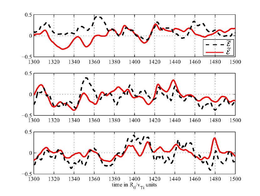
Figure 1: Time evolution of the normalized free energy $\overline{\mathcal{E}}$ associated with zonal flows and $\widetilde{\mathcal{E}}$ associated with the rest of the turbulence, for three different values of $R_{0}/L_{Ti}=6.0,6.92,8.0$ from top to bottom.

It is important to note here that it is the free energy (which corresponds to “potential enstrophy” in the fluid limit) that is exchanged between the zonal flows and the drift waves and not just the kinetic energy. The mechanism invoked here is not that of a classical “inverse cascade” but of a potential vorticity homogenization(Rhines and Young, 1982; Diamond et al., 2008), which manifests itself as disparate scale interactions in $k$-space(Krommes and Kim, 2000). Since there is no linear driving mechanism for the zonal flows (i.e. $\overline{\mathcal{G}}=0$), these structures feed on the free energy of the fluctuations and hence play the same regulating role on the underlying turbulence that a predator species plays on the population of a prey species. Figure 1 represents the time evolution of free energy ($\overline{\mathcal{E}}$ and $\widetilde{\mathcal{E}}$ have been normalized to their mean, and only a small fraction of the total time trace is represented in order to see the details of dynamics), during the turbulent phase for three values of $R_{0}/L_{Ti}=6.0,6.92,8.0$, with other parameters being those of the ITG Cyclone Base Case(Dimits et al., 2000) ($R_{0}/L_{n}=2.22$, $q=1.4$, $\hat{s}=0.796$, $r_{0}=0.18R_{0}$, and $T_{e0}=T_{i0}$). It can be observed that the free energy dynamics of the zonal flow and the turbulence are indeed largely correlated. In order to check if this dynamics exhibit predator-prey features, one can look at the phase relation between these two quantities to see if there exists a time shift between the turbulence and the zonal flow free energy fluctuations. In Figure 2, cross correlation between $\overline{\mathcal{E}}$ and $\widetilde{\mathcal{E}}$ is given as a function of the time lag. The average time delay $\Delta t$ between $\overline{\mathcal{E}}$ and $\widetilde{\mathcal{E}}$ is given by the location of the maximal correlation in Figure 2.

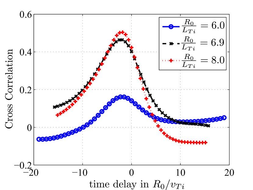
Figure 2: Cross Correlation between Zonal Flow and drift wave turbulent signals, for different values of the logarithmic temperature gradient $R_{0}/L_{Ti}$.

The predator prey type dynamics is also expected to have an intermittent nature. Therefore a look at the kurtosis is instructive: in Figure 3, the kurtosis associated with the free energy spectrum $\mathcal{E}^{k_{y}}$ is plotted as a function of $k_{y}$ for the same runs as in Figure 1. For all values of the temperature gradient, a clear separation is observed between the large and small scales, where the statistics of the small scales are very close to Gaussian (corresponding to a kurtosis of 0), while the energy containing scales associated with wave vectors $k_{y}\rho_{i}<0.5$ show a clear departure from the Gaussian distribution, suggesting the presence of rare events with significant deviation from the mean.

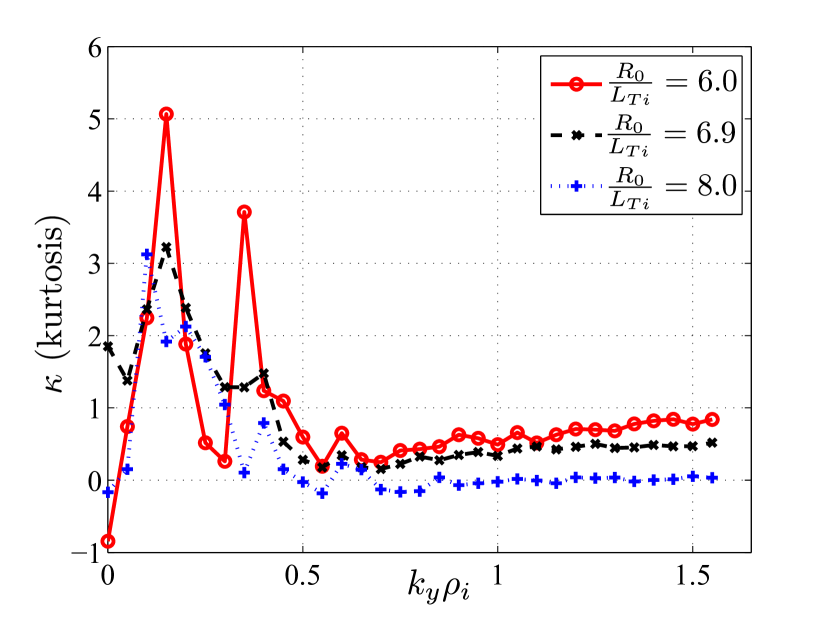
Figure 3: Free Energy kurtosis $\kappa$ as a function of the binormal wave vector $k_{y}\rho_{i}$, for different values of the logarithmic ion temperature gradient $R_{0}/L_{Ti}$.

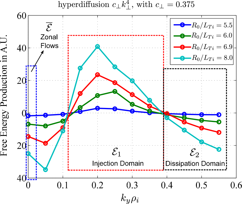
Figure 4: Free energy spectrum $\mathcal{E}^{k_{y}}$ for different values of the ion temperature gradient $R_{0}/L_{Ti}$.

While the usual predator prey model already gives interesting perspective on the dynamics the fact that the predator-prey oscillations has the character of pulses in the $k$-space transfer has to be considered also. Indeed, the free energy can be decomposed into the “energy containing” component (corresponding to the energy injection scales), the “dissipative” component (corresponding to the dissipative scales) and a “Zonal Flow” component. These three domains are illustrated in Figure 4, where the time averaged right hand side of the free energy equation i.e. $\mathcal{G}^{k_{y}}-\mathcal{D}^{k_{y}}$ is given for various values of the logarithmic temperature gradient $R_{0}/L_{Ti}$ (the transfer term $\mathcal{T}^{k_{y}}$ is not represented since: $\mathcal{T}^{k_{y}}=\mathcal{D}^{k_{y}}-\mathcal{G}^{k_{y}}$ (Bañón Navarro et al., 2011)). Simulations have been performed on reduced grids ($N_{x}\times N_{y}=48\times 24$) by means of the GyroLES technique(Morel et al., 2011) with a perpendicular hyperdiffusion model $c_{\perp}=0.375$.

The spectral transfer character of the predator-prey dynamics (5, 6) can be studied by using a model of the form:

$$\partial_{t}\overline{\mathcal{E}} = \overline{\mathcal{N}}-\nu_{F}\overline{\mathcal{E}}\,,$$ (7)

$$\partial_{t}\mathcal{E}_{1} = \mathcal{N}_{1}+\gamma\mathcal{E}_{1}\,,$$ (8)

$$\partial_{t}\mathcal{E}_{2} = \mathcal{N}_{2}-\nu\mathcal{E}_{2}\,,$$ (9)

where, $\mathcal{E}_{1}$ is the free energy at the injection scale, $\mathcal{E}_{2}$ is the free energy at the dissipation scale and $\overline{\mathcal{E}}$ is the zonal free energy, and we have used the definitions: $\nu_{F}=\overline{\mathcal{D}}/\overline{\mathcal{E}}$, $\gamma=(\mathcal{G}_{1}-\mathcal{D}_{1})/\mathcal{E}_{1}$ and $\nu=(\mathcal{D}_{2}-\mathcal{G}_{2})/\mathcal{E}_{2}$.

This three domain model is very similar to the model studied in Ref. Berionni and Gürcan, 2011, except here we use free energy. As recently shown by Nakata et al. the free energy contribution of the nonlinear term can be expressed as a symmetrized triad transfer function: $\mathcal{N}_{{\bf k}}=\sum_{{\bf p}}\sum_{{\bf q}}C_{{\bf k}}^{{\bf p},{\bf q}}\delta h_{{\bf k}}\delta h_{{\bf p}}\delta h_{{\bf q}}$, where $C_{{\bf k}}^{{\bf p},{\bf q}}$ is an operator converting the modified distribution function $\delta h_{k}$ into the electrostatic potential $\Phi_{k}$. This allows to write:

$$\overline{\mathcal{N}} = \overline{\lambda}\,\overline{h}h_{1}h_{2}\,,$$ (10)

$$\mathcal{N}_{1} = \lambda_{1}\,\overline{h}h_{1}h_{2}\,,$$ (11)

$$\mathcal{N}_{2} = \lambda_{2}\,\overline{h}h_{1}h_{2}\,.$$ (12)

where $h_{1}$, $h_{2}$ and $\overline{h}$ can be defined for instance using the partition $h_{S}=\sqrt{\int_{S}\mathcal{E}\left(k_{\perp}\right)d^{2}k_{\perp}}$ where the domain of integration in $k$-space is chosen to correspond to the injection, dissipation and zonal regions respectively.

Following Ref. Berionni and Gürcan, 2011, equations (7, 8, 9) can be averaged over the turbulent phase, so that time derivatives can be cancelled since the gyrokinetic simulation reaches a quasi-stationary state as shown in Figure 1. Coefficients $\lambda_{1}$, $\lambda_{2}$, $\bar{\lambda}$, $\gamma$, $\nu$ and $\nu_{F}$ are constants in time, and by eliminating the product $\langle\overline{h}h_{1}h_{2}\rangle$ in the averaged equations, the two following relations can be obtained:

$$\frac{\langle\mathcal{E}_{1}\rangle}{\langle\overline{\mathcal{E}}\rangle} = -\frac{\lambda_{1}\nu_{F}}{\bar{\lambda}\gamma}\,,$$ (13)

$$\frac{\langle\mathcal{E}_{2}\rangle}{\langle\overline{\mathcal{E}}\rangle} = \frac{\lambda_{2}\nu_{F}}{\bar{\lambda}\nu}\,.$$ (14)

The parameters $\lambda_{1}$, $\lambda_{2}$ and $\bar{\lambda}$ correspond to geometrical prefactors depending on the choice of the $k$-space partition and the $C_{{\bf k}}^{{\bf p},{\bf q}}$ that link $\Phi$ and $h$, and not on the physical parameters. In contrast, the linear growth rate corresponding to $\gamma$, the small scale dissipation term $\nu$, and the zonal flow drag $\nu_{F}$ are defined through $\mathcal{G}_{1,2}$, $\overline{\mathcal{G}}$, $\mathcal{D}_{1,2}$ and $\overline{\mathcal{D}}$, and thus are dependent on the free energy spectrum itself. Therefore, in principle the net dependence of these coefficients on physical parameters such as the temperature gradient can be quite nontrivial. This point is investigated in Figure 5, where the three parameters $\gamma$, $\nu_{F}$ and $\nu$ are represented as functions of the imposed $R_{0}/L_{Ti}$.

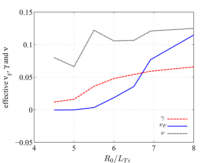
Figure 5: Effective Zonal Flows dissipation ($\nu_{F}$ , the solid line), growth rate ($\gamma$ , the dashed line) and small scale dissipation ($\nu$, the dotted line) as functions of $R_{0}/L_{Ti}$, with hyperdiffusion GyroLES ($c_{\perp}=0.5$).

In Figure 5, GyroLES simulations with various $R_{0}/L_{Ti}$ are considered, with perpendicular hyperdiffusion amplitude $c_{\perp}=0.5$. The small scale dissipation $\nu$ (dotted lines) is found approximately constant, except for small values of the temperature gradient. $\gamma$ and surprisingly $\nu_{F}$ present a nontrivial dependence with $R_{0}/L_{Ti}$, very similar to the heat flux structure found in other studies (Dimits et al., 2000).

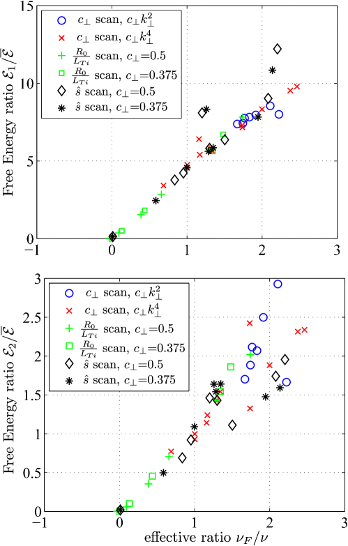
Figure 6: Free energy ratios ($\mathcal{E}_{1}/\overline{\mathcal{E}}$ top, $\mathcal{E}_{2}/\overline{\mathcal{E}}$ bottom) as functions of the ratio between the effective Zonal Flow dissipation, the effective growth rate and the effective small scale dissipation (see Eqns 13 and 14). Blue circles and red crosses stand respectively for diffusion and hyperdiffusion GyroLES model scanned along $c_{\perp}$, green plus and squares represent two $R_{0}/L_{Ti}$ scans, with respectively $c_{\perp}=0.5$ and $c_{\perp}=0.375$ chosen for hyperdiffusion GyroLES. Black diamonds and stars correspond to a magnetic shear scan $\hat{s}$ with respectively $c_{\perp}=0.5$ and $c_{\perp}=0.375$.

In order to verify Eqns. 13 and 14, , the averaged free energy ratios $\langle\mathcal{E}_{1}\rangle/\langle\overline{\mathcal{E}}\rangle$ and $\langle\mathcal{E}_{2}\rangle/\langle\overline{\mathcal{E}}\rangle$ are represented as functions of the ratios $\nu_{F}/\nu$ and $\nu_{F}/\gamma$ respectively in Figure 6. Six series of GyroLES simulations are considered, varying the diffusion or hyperdiffusion amplitudes, the temperature gradient $R_{0}/L_{Ti}$, as well as the magnetic shear, for a total of 40 nonlinear GyroLES simulations. The advantage of using LES for these simulations, (apart from the gain in speed) is that it provides an easy handle on the small scale dissipation and allows us to modify $\nu$ independently in order to explore the parameter space easily.

The curves seems to agree with the theoretically predicted ratios in Eqns. 13 and 14 . Results are however found to depart from the theory when the turbulence level is decreased, especially in the low shear case and for very high perpendicular dissipation amplitudes. The deviation of the ratio $\mathcal{E}_{1}/\overline{\mathcal{E}}$ from a straight line, is rather small, while it is more pronounced for $\mathcal{E}_{2}/\overline{\mathcal{E}}$. This could be due to the reduction of the size of the dissipative range (which affect mainly $\mathcal{E}_{2}$) by the use of the GyroLES description.

We have performed a detailed characterization of the dynamics and the associated spectral transfer, using the evolution of free energy in gyrokinetic turbulence with a partition of the $k$-space corresponding to the scales of free energy injection, free energy dissipation, and large scale flow structures. Our results show that the free energy exchange between these components exhibits, any of the well-known characteristic features of the predator-prey dynamics. We have shown that the predicted relation between the average amplitudes of these different components as given in Eqns. 13 and 14 hold reasonably well in gyrokinetic simulations.