Complex impedance, responsivity and noise of transition-edge sensors: analytical solutions for two- and three-block thermal models

I. J. Maasilta Nanoscience Center, Department of Physics, P. O. Box 35, FIN-40014 University of Jyväskylä, Finland maasilta@jyu.fi
Abstract

The responsivity and noise of a voltage-biased superconducting transition-edge sensor depends strongly on the details of its thermal model, and the simplest theory for TES response assumes a single heat capacity connected to the heat bath. Here, analytical results are derived and discussed for the complex impedance, the responsivity and the noise of a transition-edge sensor, when the thermal model is not simple but consists of either two or three connected heat capacities. The implications of the differences of the models are discussed, as well.

transition-edge sensor,thermal model,noise,complex impedance

I Introduction

Superconducting transition-edge sensors (TES) have become very popular as practical radiation detectors because of their high sensitivity and energy resolution, maturity of the fabrication technology required allowing wafer-scale processing, and versatility, so that they can be used for detection of both particles and photons from sub-millimeter frequencies to gamma-rays irwinbook . The basic operational theory of a voltage-biased TES in electrothermal feedback was described long ago irwin95 , however, in the original form the simplest possible thermal circuit was assumed, namely, that the detector could be described as a single lumped heat capacity, connected to the heat bath by a single thermal conductance. Sometimes this thermal model is fairly adequate in describing the detector response oneblock , but some detector designs have been experimentally shown to behave in a more complex manner hoevers ; zink ; NASASaab ; nasaIEEE ; mikko ; kimmo . Therefore, theoretical modeling has been advanced in recent years to include more complex thermal circuits hoevers ; galeazzi ; zink ; enectali ; appel ; takeinote ; goldie ; zhaothesis .

One way to approach the problem is to generalize the problem fully to any number of heat capacity blocks and thermal conductances, and solve the obtained (large) linearized system of equations numerically effthesis ; enectali . This approach has the advantage that it is straightforward to move from simple models to more complex models within the same formalism, and for the most complex models this may be the only approach available. Nevertheless, for models of intermediate complexity, such as systems of two or three connected heat capacities, it is possible to calculate the detector properties analytically, as well. Analytical solutions have the advantage that they are easier to work with, can be used further for fitting of experimental data, and a lot of results can be calculated quickly. One can quickly compute, for example, how the detector response changes as a function of a certain parameter of the thermal model.

Here, we present analytical solutions for the complex impedance, responsivity, and all the unavoidable components of the current noise spectral density of a TES detector, for all possible two-block thermal models and two simplest three-block models, in a compact formulation. We take advantage of the fact that we also derive the analytical equation for the complex impedance of the detector mather1 ; moseley ; linde of each model. Measurement of the complex impedance of a TES detector has been shown in recent years linde ; vailla ; zink ; linde2 to be a very valuable tool for characterising TES detectors; in particular for the discussion here, it gives information about the thermal model. There is some previously published galeazzi ; hoevers ; appel ; zhaothesis and unpublished takeinote analytical work on certain two- and three-block models of bolometers. Those results describe some limits and special cases of this work. In Refs. takeinote ; hoevers , some two-block models were discussed, and an approximation was made about the steady state temperature of the blocks. In Refs. galeazzi ; appel , equations for the impedance, responsivity and the noise equivalent power were given for one two-block and three three-block models, but the non-Ohmic behavior of the bolometer mather ; irwinbook was not fully discussed. In Ref. zhaothesis , two simple three-block models were discussed, but no simple analytical equations for the noise were given. The goal of the present work is thus to give an extensive set of equations for the responsivity, current noise and impedance in a compact and usable form, which can easily be used to analyze real noise and impedance data of TES detectors mikko ; kimmo . We also give many example plots to show how various thermal parameters affect the detector properties. Detailed discussion on the noise equivalent power, energy resolution and other figures of merit are left for future publications.

II Two-block models

We discuss here all three possible two-block cases, shown in Fig 1. One heat capacity block is always the TES film, where the Joule power is dissipated, whereas the second block describes an additional thermal body, which could represent for example the insulating membrane, the absorber etc. mikko ; kimmo ; nasaIEEE ; goldie . The formalism is kept general so that we do not need to decide on the physical picture a priori.

Refer to caption
Figure 1: All possible two-block models studied. (a) Hanging model, (b) intermediate model, (c) parallel model.

The first case, shown in Fig. 1 (a), is where the extra heat capacity C1subscript𝐶1C_{1} is connected to the TES heat capacity Ctessubscript𝐶𝑡𝑒𝑠C_{tes}, but nowhere else. This type of model has sometimes been called the hanging or dangling heat capacity model. In the second case, shown in Fig. 1 (b), the extra heat capacity lies in between the TES and the heat bath. The main difference to the first model is that now the steady state temperature of the extra block is not equal to the TES temperature, unlike in the first case of Fig. 1 (a). We call this second model the intermediate model. Finally, in the last model in Fig. 1 (c) (numerically studied in Ref. goldie ), the extra block is connected to both the TES and the heat bath as in case (b), but an additional parallel heat path exists between the TES and the bath. We call this the parallel model.

II.1 Equations to be solved

The starting point for all calculations are the differential equations that describe the heat balance in the thermal circuits and the electrical equation of the simplest Thevenin-equivalent input circuit of the TES, consisting here of an equivalent voltage Vbsubscript𝑉𝑏V_{b}, an equivalent resistance RLsubscript𝑅𝐿R_{L}, and an inductance L𝐿L in series. For a simple one-block thermal circuit, there is only one thermal equation, so that one needs to solve a coupled set of only two differential equations, as reviewed in Ref. irwinbook . They are coupled because the resistance of the TES detector R(T,I)𝑅𝑇𝐼R(T,I) depends on temperature and current, and because the Joule heating power PJsubscript𝑃𝐽P_{J} in the TES depends on the electrical parameters. It is this coupling that produces the negative electrothermal feedback in the response of a voltage biased superconducting detector irwin95 ; irwinbook . For a two-block thermal model, one additional differential equation is added to represent the extra thermal body. The exact form of the thermal equations naturally depends on which model in Fig. 1 one is analyzing. Here, we only show the equations for case (a), the hanging model, other cases follow analogously. The set of equations, excluding the noise terms for a moment, reads

CtesdTtesdtsubscript𝐶𝑡𝑒𝑠𝑑subscript𝑇𝑡𝑒𝑠𝑑𝑡\displaystyle C_{tes}\frac{dT_{tes}}{dt} =\displaystyle= PJA(TtesnT1n)B(TtesmTbm)+δP,subscript𝑃𝐽𝐴superscriptsubscript𝑇𝑡𝑒𝑠𝑛superscriptsubscript𝑇1𝑛𝐵superscriptsubscript𝑇𝑡𝑒𝑠𝑚superscriptsubscript𝑇𝑏𝑚𝛿𝑃\displaystyle P_{J}-A\left(T_{tes}^{n}-T_{1}^{n}\right)-B\left(T_{tes}^{m}-T_{b}^{m}\right)+\delta P,
C1dT1dtsubscript𝐶1𝑑subscript𝑇1𝑑𝑡\displaystyle C_{1}\frac{dT_{1}}{dt} =\displaystyle= A(TtesnT1n),𝐴superscriptsubscript𝑇𝑡𝑒𝑠𝑛superscriptsubscript𝑇1𝑛\displaystyle A\left(T_{tes}^{n}-T_{1}^{n}\right),
LdIdt𝐿𝑑𝐼𝑑𝑡\displaystyle L\frac{dI}{dt} =\displaystyle= VbIRLIR(Ttes,I),subscript𝑉𝑏𝐼subscript𝑅𝐿𝐼𝑅subscript𝑇𝑡𝑒𝑠𝐼\displaystyle V_{b}-IR_{L}-IR(T_{tes},I), (1)

where Ttessubscript𝑇𝑡𝑒𝑠T_{tes} and T1subscript𝑇1T_{1} are the instantaneous temperatures of the TES and the extra heat capacity, respectively, and the heat bath is at a temperature Tbsubscript𝑇𝑏T_{b}. A𝐴A and B𝐵B are constants describing the strength of the thermal links between the TES and C1subscript𝐶1C_{1}, and TES and heat bath, respectively, and n𝑛n and m𝑚m are temperature exponents, which depend on the physical nature of the thermal links irwinbook . δP𝛿𝑃\delta P, on the other hand, is some time-dependent power input to the TES. Using these equations, the full time-dependent response (temperature and current) could, in principle, be solved. However, the power flows are non-linear functions of temperature, and the TES resistance is a non-linear function of both T𝑇T and I𝐼I, so that an analytical solution for the system is not tractable in the general (large signal) case. In this work, however, we are only interested in the impedance, noise and responsivity, all of which are traditionally defined only in the small-signal limit, where the non-linearities can be ignored. The linearization of Eqs. 1 is done by the usual Taylor expansions around steady state values irwinbook (denoted by subscript 00):

IR(Ttes,I)𝐼𝑅subscript𝑇𝑡𝑒𝑠𝐼\displaystyle IR(T_{tes},I) \displaystyle\approx I0R0+αI0(R0/Ttes,0)ΔTtes+(1+β)R0ΔI,subscript𝐼0subscript𝑅0𝛼subscript𝐼0subscript𝑅0subscript𝑇𝑡𝑒𝑠0Δsubscript𝑇𝑡𝑒𝑠1𝛽subscript𝑅0Δ𝐼\displaystyle I_{0}R_{0}+\alpha I_{0}(R_{0}/T_{tes,0})\Delta T_{tes}+(1+\beta)R_{0}\Delta I,
PJsubscript𝑃𝐽\displaystyle P_{J} \displaystyle\approx P0+[2I0R0+β(P0/I0)]ΔI+α(P0/Ttes,0)ΔTtes,subscript𝑃0delimited-[]2subscript𝐼0subscript𝑅0𝛽subscript𝑃0subscript𝐼0Δ𝐼𝛼subscript𝑃0subscript𝑇𝑡𝑒𝑠0Δsubscript𝑇𝑡𝑒𝑠\displaystyle P_{0}+[2I_{0}R_{0}+\beta(P_{0}/I_{0})]\Delta I+\alpha(P_{0}/T_{tes,0})\Delta T_{tes},
A(TtesnT1n)𝐴superscriptsubscript𝑇𝑡𝑒𝑠𝑛superscriptsubscript𝑇1𝑛\displaystyle A(T_{tes}^{n}-T_{1}^{n}) \displaystyle\approx A(Ttes,0nT1,0n)+nATtes,0n1ΔTtesnAT1,0n1ΔT1,𝐴superscriptsubscript𝑇𝑡𝑒𝑠0𝑛superscriptsubscript𝑇10𝑛𝑛𝐴superscriptsubscript𝑇𝑡𝑒𝑠0𝑛1Δsubscript𝑇𝑡𝑒𝑠𝑛𝐴superscriptsubscript𝑇10𝑛1Δsubscript𝑇1\displaystyle A(T_{tes,0}^{n}-T_{1,0}^{n})+nAT_{tes,0}^{n-1}\Delta T_{tes}-nAT_{1,0}^{n-1}\Delta T_{1},
B(TtesmTbm)𝐵superscriptsubscript𝑇𝑡𝑒𝑠𝑚superscriptsubscript𝑇𝑏𝑚\displaystyle B(T_{tes}^{m}-T_{b}^{m}) \displaystyle\approx B(Ttes,0mTbm)+mBTtes,0m1ΔTtes,𝐵superscriptsubscript𝑇𝑡𝑒𝑠0𝑚superscriptsubscript𝑇𝑏𝑚𝑚𝐵superscriptsubscript𝑇𝑡𝑒𝑠0𝑚1Δsubscript𝑇𝑡𝑒𝑠\displaystyle B(T_{tes,0}^{m}-T_{b}^{m})+mBT_{tes,0}^{m-1}\Delta T_{tes}, (2)

where ΔTtes=TtesTtes,0Δsubscript𝑇𝑡𝑒𝑠subscript𝑇𝑡𝑒𝑠subscript𝑇𝑡𝑒𝑠0\Delta T_{tes}=T_{tes}-T_{tes,0}, ΔI=II0Δ𝐼𝐼subscript𝐼0\Delta I=I-I_{0}, ΔT1=T1T1,0Δsubscript𝑇1subscript𝑇1subscript𝑇10\Delta T_{1}=T_{1}-T_{1,0}, and α=(Ttes,0/R0)(R/T)|I0𝛼evaluated-atsubscript𝑇𝑡𝑒𝑠0subscript𝑅0𝑅𝑇subscript𝐼0\alpha=(T_{tes,0}/R_{0})(\partial R/\partial T)|_{I_{0}} and β=(I0/R0)(R/I)|Ttes,0𝛽evaluated-atsubscript𝐼0subscript𝑅0𝑅𝐼subscript𝑇𝑡𝑒𝑠0\beta=(I_{0}/R_{0})(\partial R/\partial I)|_{T_{tes,0}} are the dimensionless (logarithmic) transition sensitivity parameters. Substituting the above expansions into Eqs. 1 lead to the linearized set of equations

CtesdΔTtesdtsubscript𝐶𝑡𝑒𝑠𝑑Δsubscript𝑇𝑡𝑒𝑠𝑑𝑡\displaystyle C_{tes}\frac{d\Delta T_{tes}}{dt} =\displaystyle= (2I0R0+βP0I0)ΔI+(αP0Ttes,0gtes,1gtes,b)ΔTtes+gtes,1ΔT1+δP,2subscript𝐼0subscript𝑅0𝛽subscript𝑃0subscript𝐼0Δ𝐼𝛼subscript𝑃0subscript𝑇𝑡𝑒𝑠0subscript𝑔𝑡𝑒𝑠1subscript𝑔𝑡𝑒𝑠𝑏Δsubscript𝑇𝑡𝑒𝑠subscript𝑔𝑡𝑒𝑠1Δsubscript𝑇1𝛿𝑃\displaystyle\left(2I_{0}R_{0}+\beta\frac{P_{0}}{I_{0}}\right)\Delta I+\left(\alpha\frac{P_{0}}{T_{tes,0}}-g_{tes,1}-g_{tes,b}\right)\Delta T_{tes}+g_{tes,1}\Delta T_{1}+\delta P,
C1dΔT1dtsubscript𝐶1𝑑Δsubscript𝑇1𝑑𝑡\displaystyle C_{1}\frac{d\Delta T_{1}}{dt} =\displaystyle= gtes,1(ΔTtesΔT1),subscript𝑔𝑡𝑒𝑠1Δsubscript𝑇𝑡𝑒𝑠Δsubscript𝑇1\displaystyle g_{tes,1}\left(\Delta T_{tes}-\Delta T_{1}\right),
LdΔIdt𝐿𝑑Δ𝐼𝑑𝑡\displaystyle L\frac{d\Delta I}{dt} =\displaystyle= δVbΔIRLαI0R0Ttes,0ΔTtes(1+β)R0ΔI,𝛿subscript𝑉𝑏Δ𝐼subscript𝑅𝐿𝛼subscript𝐼0subscript𝑅0subscript𝑇𝑡𝑒𝑠0Δsubscript𝑇𝑡𝑒𝑠1𝛽subscript𝑅0Δ𝐼\displaystyle\delta V_{b}-\Delta IR_{L}-\alpha\frac{I_{0}R_{0}}{T_{tes,0}}\Delta T_{tes}-(1+\beta)R_{0}\Delta I, (3)

where we have defined the differential thermal conductances gtes,1=nATtes,0n1subscript𝑔𝑡𝑒𝑠1𝑛𝐴superscriptsubscript𝑇𝑡𝑒𝑠0𝑛1g_{tes,1}=nAT_{tes,0}^{n-1} and gtes,b=mBTtes,0m1subscript𝑔𝑡𝑒𝑠𝑏𝑚𝐵superscriptsubscript𝑇𝑡𝑒𝑠0𝑚1g_{tes,b}=mBT_{tes,0}^{m-1}, and used the fact that for the hanging model T1,0=Ttes,0subscript𝑇10subscript𝑇𝑡𝑒𝑠0T_{1,0}=T_{tes,0}. From now on, we also simplify the notation as T0Ttes,0subscript𝑇0subscript𝑇𝑡𝑒𝑠0T_{0}\equiv T_{tes,0}. Also, after linearization, one can ignore the temperature dependence of the heat capacities and consider them to be constants [Ctes=Ctes(T0)subscript𝐶𝑡𝑒𝑠subscript𝐶𝑡𝑒𝑠subscript𝑇0C_{tes}=C_{tes}(T_{0}), C1=C1(T0)subscript𝐶1subscript𝐶1subscript𝑇0C_{1}=C_{1}(T_{0}) ], as the corrections are in second order effthesis .

Eqs. 3 have been analyzed in time-domain in Ref bennett , with focus on pulse response and electrothermal stability analysis. Here, we proceed to focus on the frequency domain (also discussed in Ref. takeinote for this model), which is natural for impedance and noise analysis. Fourier transforming Eqs. 3 and simplifying notation, one gets

iωTω,tes𝑖𝜔subscript𝑇𝜔𝑡𝑒𝑠\displaystyle i\omega T_{\omega,tes} =\displaystyle= I0R0(2+β)CtesIω1τITω,tes+1τtes,1Tω,1+1CtesPω,subscript𝐼0subscript𝑅02𝛽subscript𝐶𝑡𝑒𝑠subscript𝐼𝜔1subscript𝜏𝐼subscript𝑇𝜔𝑡𝑒𝑠1subscript𝜏𝑡𝑒𝑠1subscript𝑇𝜔11subscript𝐶𝑡𝑒𝑠subscript𝑃𝜔\displaystyle\frac{I_{0}R_{0}(2+\beta)}{C_{tes}}I_{\omega}-\frac{1}{\tau_{I}}T_{\omega,tes}+\frac{1}{\tau_{tes,1}}T_{\omega,1}+\frac{1}{C_{tes}}P_{\omega},
iωTω,1𝑖𝜔subscript𝑇𝜔1\displaystyle i\omega T_{\omega,1} =\displaystyle= 1τ1(Tω,tesTω,1)1subscript𝜏1subscript𝑇𝜔𝑡𝑒𝑠subscript𝑇𝜔1\displaystyle\frac{1}{\tau_{1}}\left(T_{\omega,tes}-T_{\omega,1}\right)
iωLIω𝑖𝜔𝐿subscript𝐼𝜔\displaystyle i\omega LI_{\omega} =\displaystyle= Vω[RL+R0(1+β)]IωH(gtes,1+gtes,b)I0Tω,tes,subscript𝑉𝜔delimited-[]subscript𝑅𝐿subscript𝑅01𝛽subscript𝐼𝜔subscript𝐻subscript𝑔𝑡𝑒𝑠1subscript𝑔𝑡𝑒𝑠𝑏subscript𝐼0subscript𝑇𝜔𝑡𝑒𝑠\displaystyle V_{\omega}-\left[R_{L}+R_{0}(1+\beta)\right]I_{\omega}-\frac{{\cal L}_{H}(g_{tes,1}+g_{tes,b})}{I_{0}}T_{\omega,tes}, (4)

where we have denoted the Fourier amplitudes of all variables as Xωsubscript𝑋𝜔X_{\omega}, have defined τtes,1=Ctes/gtes,1subscript𝜏𝑡𝑒𝑠1subscript𝐶𝑡𝑒𝑠subscript𝑔𝑡𝑒𝑠1\tau_{tes,1}=C_{tes}/g_{tes,1}, and have defined two other important time constants and a dimensionless quantity Hsubscript𝐻{\cal L}_{H} that appears in the place of the loop gain of the simple model as

τIsubscript𝜏𝐼\displaystyle\tau_{I} =\displaystyle= Ctes(gtes,1+gtes,b)(1H),subscript𝐶𝑡𝑒𝑠subscript𝑔𝑡𝑒𝑠1subscript𝑔𝑡𝑒𝑠𝑏1subscript𝐻\displaystyle\frac{C_{tes}}{(g_{tes,1}+g_{tes,b})(1-{\cal L}_{H})},
τ1subscript𝜏1\displaystyle\tau_{1} =\displaystyle= C1gtes,1,subscript𝐶1subscript𝑔𝑡𝑒𝑠1\displaystyle\frac{C_{1}}{g_{tes,1}},
Hsubscript𝐻\displaystyle{\cal L}_{H} =\displaystyle= P0α(gtes,1+gtes,b)T0.subscript𝑃0𝛼subscript𝑔𝑡𝑒𝑠1subscript𝑔𝑡𝑒𝑠𝑏subscript𝑇0\displaystyle\frac{P_{0}\alpha}{(g_{tes,1}+g_{tes,b})T_{0}}. (5)

Note that the definition of this ”effective loop gain” Hsubscript𝐻{\cal L}_{H} here is different from the standard one-block model one irwinbook =P0α/(gtes,bT0)subscript𝑃0𝛼subscript𝑔𝑡𝑒𝑠𝑏subscript𝑇0{\cal L}=P_{0}\alpha/(g_{tes,b}T_{0}), and therefore H=gtes,b/(gtes,1+gtes,b)subscript𝐻subscript𝑔𝑡𝑒𝑠𝑏subscript𝑔𝑡𝑒𝑠1subscript𝑔𝑡𝑒𝑠𝑏{\cal L}_{H}=g_{tes,b}/(g_{tes,1}+g_{tes,b}){\cal L}. In fact, if one calculates the true zero frequency, perfect voltage bias loop gain starting from the definitions mccammonbook , one arrives at {\cal L} even for this hanging model. This is intuitive, as the coupling to bath is the same. However, the new definition does have the benefit that for each different model (hanging, intermediate or parallel), the equations 4 have the same mathematical form, only the definition of the effective loop gain and the time constants change, as will be seen later. It is, of course, still possible to work with other, less compact notations, as was done for example in Refs. bennett ; takeinote ; zhaothesis .

II.2 Complex impedance

II.2.1 Hanging model

The first quantity we want to derive from Eqs. 4 for the hanging model is the frequency dependent complex impedance of the TES, Ztes,Hsubscript𝑍𝑡𝑒𝑠𝐻Z_{tes,H}. As the full circuit impedance Zcircsubscript𝑍𝑐𝑖𝑟𝑐Z_{circ} is calculated by Zcirc=Vω/Iωsubscript𝑍𝑐𝑖𝑟𝑐subscript𝑉𝜔subscript𝐼𝜔Z_{circ}=V_{\omega}/I_{\omega}, we can subtract from it the known impedance of the circuit outside of the TES to define Ztes=ZcircRLiωLsubscript𝑍𝑡𝑒𝑠subscript𝑍𝑐𝑖𝑟𝑐subscript𝑅𝐿𝑖𝜔𝐿Z_{tes}=Z_{circ}-R_{L}-i\omega L for the simplest bias circuit case, or Ztes=ZcircZbiassubscript𝑍𝑡𝑒𝑠subscript𝑍𝑐𝑖𝑟𝑐subscript𝑍𝑏𝑖𝑎𝑠Z_{tes}=Z_{circ}-Z_{bias} in general. We can set Pω=0subscript𝑃𝜔0P_{\omega}=0, and obtain

Ztes,H=R0(1+β)+H1HR0(2+β)/[1+iωτIgtes,1(gtes,1+gtes,b)(1H)11+iωτ1],subscript𝑍𝑡𝑒𝑠𝐻subscript𝑅01𝛽/subscript𝐻1subscript𝐻subscript𝑅02𝛽delimited-[]1𝑖𝜔subscript𝜏𝐼subscript𝑔𝑡𝑒𝑠1subscript𝑔𝑡𝑒𝑠1subscript𝑔𝑡𝑒𝑠𝑏1subscript𝐻11𝑖𝜔subscript𝜏1Z_{tes,H}=R_{0}(1+\beta)+\frac{{\cal L}_{H}}{1-{\cal L}_{H}}R_{0}(2+\beta)\left/\left[1+i\omega\tau_{I}-\frac{g_{tes,1}}{(g_{tes,1}+g_{tes,b})(1-{\cal L}_{H})}\frac{1}{1+i\omega\tau_{1}}\right]\right., (6)

with definitions of Hsubscript𝐻{\cal L}_{H}, τIsubscript𝜏𝐼\tau_{I} and τ1subscript𝜏1\tau_{1} given in Eqs. 5. This can be compared with the result for the simple one-block model irwinbook

Ztes=R0(1+β)+1R0(2+β)11+iωτI,subscript𝑍𝑡𝑒𝑠subscript𝑅01𝛽1subscript𝑅02𝛽11𝑖𝜔subscript𝜏𝐼Z_{tes}=R_{0}(1+\beta)+\frac{{\cal L}}{1-{\cal L}}R_{0}(2+\beta)\frac{1}{1+i\omega\tau_{I}}, (7)

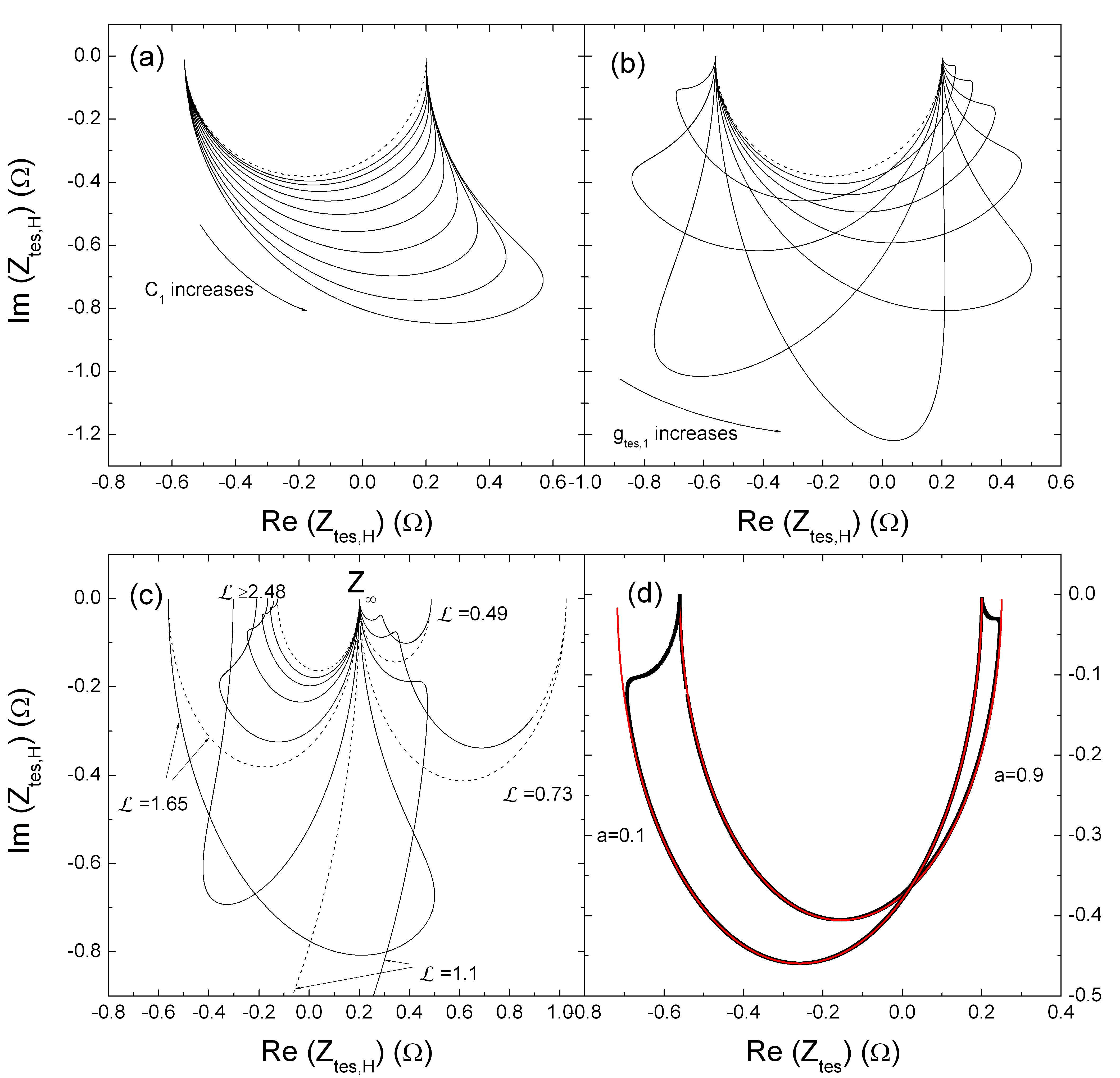
where τI=Ctes/[gtes,b(1)]subscript𝜏𝐼subscript𝐶𝑡𝑒𝑠delimited-[]subscript𝑔𝑡𝑒𝑠𝑏1\tau_{I}=C_{tes}/[g_{tes,b}(1-{\cal L})] for the one-block model. We see that due to the second heat capacity, a new frequency-dependent term with time constant τ1subscript𝜏1\tau_{1} appears in the denominator. Thus, the effect of C1subscript𝐶1C_{1} is non-linear. The strength of the extra term is not only set by the value of C1subscript𝐶1C_{1}, but also by how large the thermal conductance gtes,1subscript𝑔𝑡𝑒𝑠1g_{tes,1} is relative to gtes,bsubscript𝑔𝑡𝑒𝑠𝑏g_{tes,b}. However, as the effective loop gain Hsubscript𝐻{\cal L}_{H} also depends on the ratio of the two thermal conductances, it turns out that Ztes,Hsubscript𝑍𝑡𝑒𝑠𝐻Z_{tes,H} deviates maximally in the complex plane from the simple model for some value a=gtes,1/(gtes,1+gtes,b)<1𝑎subscript𝑔𝑡𝑒𝑠1subscript𝑔𝑡𝑒𝑠1subscript𝑔𝑡𝑒𝑠𝑏1a=g_{tes,1}/(g_{tes,1}+g_{tes,b})<1, depending on the value of loop gain. In the limits a0𝑎0a\rightarrow 0 and a1𝑎1a\rightarrow 1, Ztes,Hsubscript𝑍𝑡𝑒𝑠𝐻Z_{tes,H} approaches the simple one-block model result, with a heat capacity Ctessubscript𝐶𝑡𝑒𝑠C_{tes} and Ctes+C1subscript𝐶𝑡𝑒𝑠subscript𝐶1C_{tes}+C_{1}, respectively. We show some example plots of the effects of C1subscript𝐶1C_{1} and gtes,1subscript𝑔𝑡𝑒𝑠1g_{tes,1} in Fig. 2. We see that increasing C1subscript𝐶1C_{1} distorts Ztes,Hsubscript𝑍𝑡𝑒𝑠𝐻Z_{tes,H} more from the simple-model half-circle [Fig. 2 (a)], but keeps the direction of the extra ”bulge” constant in the complex plane. Changing gtes,1subscript𝑔𝑡𝑒𝑠1g_{tes,1}, on the other hand, changes both the location and the size of the ”bulge” feature. The loop gain also has a direct and quite complex effect, as shown in Fig. 2 (c). In the large loop gain limit, the two-block hanging model approaches the simple model, but for typical values of {\cal L} the effect of the extra term is strong, and, interestingly, remains even in the limit 00{\cal L}\rightarrow 0. For 0<<1010<{\cal L}<1, the effect of the two-block model is opposite compared to >11{\cal L}>1, in that the circular shape of the simple model is distorted inward.
Refer to caption
Figure 2: (Color online) Complex impedance of a two-block hanging model, with varying parameters. We have used R0=0.1Ωsubscript𝑅00.1ΩR_{0}=0.1{\mathrm{\Omega}} and β=1𝛽1\beta=1 in all plots, and frequencies run typically between ωτtes=0.01..100𝜔subscript𝜏𝑡𝑒𝑠0.01..100\omega\tau_{tes}=0.01..100, where τtes=Ctes/gtes,bsubscript𝜏𝑡𝑒𝑠subscript𝐶𝑡𝑒𝑠subscript𝑔𝑡𝑒𝑠𝑏\tau_{tes}=C_{tes}/g_{tes,b}. (a) Ztes,Hsubscript𝑍𝑡𝑒𝑠𝐻Z_{tes,H} as a function of C1subscript𝐶1C_{1}, with C1/Ctes=0.33,0.49,0.73,1.1,1.65,2.48,3.71,5.57,8.35,12.5subscript𝐶1subscript𝐶𝑡𝑒𝑠0.330.490.731.11.652.483.715.578.3512.5C_{1}/C_{tes}=0.33,0.49,0.73,1.1,1.65,2.48,3.71,5.57,8.35,12.5, =1.651.65{\cal L}=1.65 and a=gtes,1/(gtes,1+gtes,b)=0.5𝑎subscript𝑔𝑡𝑒𝑠1subscript𝑔𝑡𝑒𝑠1subscript𝑔𝑡𝑒𝑠𝑏0.5a=g_{tes,1}/(g_{tes,1}+g_{tes,b})=0.5. Increasing C1subscript𝐶1C_{1} corresponds to a larger deviation from the one-block model, shown as dashed line. (b) Ztes,Hsubscript𝑍𝑡𝑒𝑠𝐻Z_{tes,H} as a function of a𝑎a ( gtes,1subscript𝑔𝑡𝑒𝑠1g_{tes,1}), with a=0.1,0.2,0.3,0.4,0.5,0.6,0.7,0.8,0.9𝑎0.10.20.30.40.50.60.70.80.9a=0.1,0.2,0.3,0.4,0.5,0.6,0.7,0.8,0.9, =1.651.65{\cal L}=1.65 and C1/Ctes=10subscript𝐶1subscript𝐶𝑡𝑒𝑠10C_{1}/C_{tes}=10. Increasing a𝑎a corresponds to the bulge feature moving from the left, low-frequency side to the right, high-frequency side. Dashed line is the one-block model limit (a0𝑎0a\rightarrow 0). (c) Ztes,Hsubscript𝑍𝑡𝑒𝑠𝐻Z_{tes,H} as a function of =P0α/(gtes,bT0)subscript𝑃0𝛼subscript𝑔𝑡𝑒𝑠𝑏subscript𝑇0{\cal L}=P_{0}\alpha/(g_{tes,b}T_{0}), with =0.49,0.73,1.1,1.65,2.48,3.71,5.57,8.35,12.50.490.731.11.652.483.715.578.3512.5{\cal L}=0.49,0.73,1.1,1.65,2.48,3.71,5.57,8.35,12.5, C1/Ctes=10subscript𝐶1subscript𝐶𝑡𝑒𝑠10C_{1}/C_{tes}=10 and a=0.5𝑎0.5a=0.5. Dashed lines show the corresponding one-block results. (d) Comparison of two Ztes,Hsubscript𝑍𝑡𝑒𝑠𝐻Z_{tes,H} impedance curves (points) (C1/Ctes=10subscript𝐶1subscript𝐶𝑡𝑒𝑠10C_{1}/C_{tes}=10, =1.651.65{\cal L}=1.65 and either a=0.1𝑎0.1a=0.1 or a=0.9𝑎0.9a=0.9) with one-block model fits (red lines). For a=0.9𝑎0.9a=0.9, the one-block fitted parameters are β=1.5𝛽1.5\beta=1.5, =1.761.76{\cal L}=1.76 and C=12Ctes𝐶12subscript𝐶𝑡𝑒𝑠C=12C_{tes}, whereas for a=0.1𝑎0.1a=0.1, we get fitted values =1.4851.485{\cal L}=1.485 and C=0.9Ctes𝐶0.9subscript𝐶𝑡𝑒𝑠C=0.9C_{tes}, with β=1𝛽1\beta=1 kept fixed.

In Fig. 2 (d) we show two examples of a potential pitfall in analyzing impedance data. In the limits where gtes,1subscript𝑔𝑡𝑒𝑠1g_{tes,1} is either clearly smaller or clearly larger than gtes,bsubscript𝑔𝑡𝑒𝑠𝑏g_{tes,b}, the shape of Ztes,Hsubscript𝑍𝑡𝑒𝑠𝐻Z_{tes,H} is only distorted at the low-frequency or high-frequency end, respectively. In that case, an incomplete frequency range of the data could lead to a misinterpretation of a two-block model as a one-block model. For example, in Fig. 2 (d) we show a plot of a two-block model with a=0.9𝑎0.9a=0.9, β=1𝛽1\beta=1, =1.651.65{\cal L}=1.65, and C1/Ctes=10subscript𝐶1subscript𝐶𝑡𝑒𝑠10C_{1}/C_{tes}=10, which can be fitted with a one-block model up to a frequency ωτtes2similar-to𝜔subscript𝜏𝑡𝑒𝑠2\omega\tau_{tes}\sim 2, but with misidentified β=1.5𝛽1.5\beta=1.5, =1.761.76{\cal L}=1.76 and C=12Ctes𝐶12subscript𝐶𝑡𝑒𝑠C=12C_{tes}. The same way, the two-block impedance with a=0.1𝑎0.1a=0.1 (other parameters the same) can be fitted with a one-block model with misidentified =1.4851.485{\cal L}=1.485 and C=0.9Ctes𝐶0.9subscript𝐶𝑡𝑒𝑠C=0.9C_{tes}, down to a frequency ωτtes0.05similar-to𝜔subscript𝜏𝑡𝑒𝑠0.05\omega\tau_{tes}\sim 0.05. The high-frequency distortions can get especially tricky, as measurements always have an electrical high-frequency cut-off somewhere.

II.2.2 Intermediate model

Turning to the second, intermediate model (Fig. 1 (b)), we can follow similar derivation as for the hanging model. Omitting details, we find the same mathematical form for Ztessubscript𝑍𝑡𝑒𝑠Z_{tes}, but with different definitions of the effective loop gain and time constants:

Ztes,IM=R0(1+β)+IM1IMR0(2+β)/[1+iωτIgtes,1(T1)[gtes,1(T1)+g1,b](1IM)11+iωτ1],subscript𝑍𝑡𝑒𝑠𝐼𝑀subscript𝑅01𝛽/subscript𝐼𝑀1subscript𝐼𝑀subscript𝑅02𝛽delimited-[]1𝑖𝜔subscript𝜏𝐼subscript𝑔𝑡𝑒𝑠1subscript𝑇1delimited-[]subscript𝑔𝑡𝑒𝑠1subscript𝑇1subscript𝑔1𝑏1subscript𝐼𝑀11𝑖𝜔subscript𝜏1Z_{tes,IM}=R_{0}(1+\beta)+\frac{{\cal L}_{IM}}{1-{\cal L}_{IM}}R_{0}(2+\beta)\left/\left[1+i\omega\tau_{I}-\frac{g_{tes,1}(T_{1})}{[g_{tes,1}(T_{1})+g_{1,b}](1-{\cal L}_{IM})}\frac{1}{1+i\omega\tau_{1}}\right]\right., (8)

where

τIsubscript𝜏𝐼\displaystyle\tau_{I} =\displaystyle= Ctesgtes,1(T0)(1IM)subscript𝐶𝑡𝑒𝑠subscript𝑔𝑡𝑒𝑠1subscript𝑇01subscript𝐼𝑀\displaystyle\frac{C_{tes}}{g_{tes,1}(T_{0})(1-{\cal L}_{IM})}
τ1subscript𝜏1\displaystyle\tau_{1} =\displaystyle= C1gtes,1(T1)+g1,bsubscript𝐶1subscript𝑔𝑡𝑒𝑠1subscript𝑇1subscript𝑔1𝑏\displaystyle\frac{C_{1}}{g_{tes,1}(T_{1})+g_{1,b}}
IMsubscript𝐼𝑀\displaystyle{\cal L}_{IM} =\displaystyle= P0αgtes,1(T0)T0.subscript𝑃0𝛼subscript𝑔𝑡𝑒𝑠1subscript𝑇0subscript𝑇0\displaystyle\frac{P_{0}\alpha}{g_{tes,1}(T_{0})T_{0}}. (9)

Here, we must also explicitly define at what temperature gtes,1subscript𝑔𝑡𝑒𝑠1g_{tes,1} is evaluated, as the two blocks have different steady-state temperatures in this case (T0subscript𝑇0T_{0} for Ctessubscript𝐶𝑡𝑒𝑠C_{tes} and T1subscript𝑇1T_{1} for C1subscript𝐶1C_{1}), and therefore there are two different values for gtes,1subscript𝑔𝑡𝑒𝑠1g_{tes,1} that come into play: gtes,1(T1)subscript𝑔𝑡𝑒𝑠1subscript𝑇1g_{tes,1}(T_{1}) and gtes,1(T0)subscript𝑔𝑡𝑒𝑠1subscript𝑇0g_{tes,1}(T_{0}). g1,bsubscript𝑔1𝑏g_{1,b} is always evaluated at T1subscript𝑇1T_{1}, and is therefore not explicitly written in the above equations for simplification. g1,b(Tb)subscript𝑔1𝑏subscript𝑇𝑏g_{1,b}(T_{b}) will only come into play when calculating noise (Sect. II.4).

Eq. 8 thus shows that the complex impedance of the intermediate model behaves qualitatively exactly like the hanging model one, so that similar plots to Fig. 2 can be generated, but with different parameter values. It is therefore very hard, if not impossible, to distinguish between the hanging and intermediate models based on fitting impedance data alone, as was pointed out in Refs. takeinote ; lindeIEEE already.

In the intermediate model, it is clear that the true loop gain is really different from the simple model, unlike in the hanging case, as the extra block affects the DC response. One way to find the loop gain is to look at the zero frequency limit of Eq. 8. Doing that, one finds =P0α/(geffT0)subscript𝑃0𝛼subscript𝑔𝑒𝑓𝑓subscript𝑇0{\cal L}=P_{0}\alpha/(g_{eff}T_{0}), where

geff=gtes,1(T0)g1,bgtes,1(T1)+g1,bsubscript𝑔𝑒𝑓𝑓subscript𝑔𝑡𝑒𝑠1subscript𝑇0subscript𝑔1𝑏subscript𝑔𝑡𝑒𝑠1subscript𝑇1subscript𝑔1𝑏g_{eff}=\frac{g_{tes,1}(T_{0})g_{1,b}}{g_{tes,1}(T_{1})+g_{1,b}} (10)

is an effective differential thermal conductance, which is a series combination of the two individual thermal conductances. Notice, though, how gtes,1subscript𝑔𝑡𝑒𝑠1g_{tes,1} has to be evaluated at different temperatures in the nominator and in the denominator. The added complication for analysis is that if T1subscript𝑇1T_{1} is not directly measurable (typical case), then the DC I-V measurements alone cannot fix T0subscript𝑇0T_{0} or the parameters A𝐴A, B𝐵B, n𝑛n and m𝑚m, as there are too many unknowns in the general case. Only if one can set n=m𝑛𝑚n=m based on physical assumptions (same thermal conduction mechanism), can one determine both T0subscript𝑇0T_{0} and geffsubscript𝑔𝑒𝑓𝑓g_{eff} from the I-V data. T1subscript𝑇1T_{1} naturally depends on the relative strength of the two thermal conductances such that if n=m𝑛𝑚n=m,

T1=(gtes,1(T1)gtes,1(T1)+g1,bT0n+g1,bgtes,1(T1)+g1,bTbn)1/n.subscript𝑇1superscriptsubscript𝑔𝑡𝑒𝑠1subscript𝑇1subscript𝑔𝑡𝑒𝑠1subscript𝑇1subscript𝑔1𝑏superscriptsubscript𝑇0𝑛subscript𝑔1𝑏subscript𝑔𝑡𝑒𝑠1subscript𝑇1subscript𝑔1𝑏superscriptsubscript𝑇𝑏𝑛1𝑛T_{1}=\left(\frac{g_{tes,1}(T_{1})}{g_{tes,1}(T_{1})+g_{1,b}}T_{0}^{n}+\frac{g_{1,b}}{g_{tes,1}(T_{1})+g_{1,b}}T_{b}^{n}\right)^{1/n}. (11)

II.2.3 Parallel model

Finally, we discuss the third and final two-block model, where both blocks have conduction channels to the bath, the parallel model [Fig. 1 (c)]. Again, it is straightforward to derive equations analogous to Eqs. 4 and to solve for Ztessubscript𝑍𝑡𝑒𝑠Z_{tes}, yielding once again the same form

Ztes,Psubscript𝑍𝑡𝑒𝑠𝑃\displaystyle Z_{tes,P} =\displaystyle= R0(1+β)+P1PR0(2+β)/\displaystyle R_{0}(1+\beta)+\frac{{\cal L}_{P}}{1-{\cal L}_{P}}R_{0}(2+\beta)/ (12)
[1+iωτIgtes,1(T0)gtes,1(T1)[gtes,1(T0)+gtes,b][gtes,1(T1)+g1,b](1P)11+iωτ1],delimited-[]1𝑖𝜔subscript𝜏𝐼subscript𝑔𝑡𝑒𝑠1subscript𝑇0subscript𝑔𝑡𝑒𝑠1subscript𝑇1delimited-[]subscript𝑔𝑡𝑒𝑠1subscript𝑇0subscript𝑔𝑡𝑒𝑠𝑏delimited-[]subscript𝑔𝑡𝑒𝑠1subscript𝑇1subscript𝑔1𝑏1subscript𝑃11𝑖𝜔subscript𝜏1\displaystyle\left[1+i\omega\tau_{I}-\frac{g_{tes,1}(T_{0})g_{tes,1}(T_{1})}{[g_{tes,1}(T_{0})+g_{tes,b}][g_{tes,1}(T_{1})+g_{1,b}](1-{\cal L}_{P})}\frac{1}{1+i\omega\tau_{1}}\right],

with definitions

τIsubscript𝜏𝐼\displaystyle\tau_{I} =\displaystyle= Ctes(gtes,1(T0)+gtes,b)(1P)subscript𝐶𝑡𝑒𝑠subscript𝑔𝑡𝑒𝑠1subscript𝑇0subscript𝑔𝑡𝑒𝑠𝑏1subscript𝑃\displaystyle\frac{C_{tes}}{(g_{tes,1}(T_{0})+g_{tes,b})(1-{\cal L}_{P})}
τ1subscript𝜏1\displaystyle\tau_{1} =\displaystyle= C1gtes,1(T1)+g1,bsubscript𝐶1subscript𝑔𝑡𝑒𝑠1subscript𝑇1subscript𝑔1𝑏\displaystyle\frac{C_{1}}{g_{tes,1}(T_{1})+g_{1,b}}
Psubscript𝑃\displaystyle{\cal L}_{P} =\displaystyle= P0α(gtes,1(T0)+gtes,b)T0.subscript𝑃0𝛼subscript𝑔𝑡𝑒𝑠1subscript𝑇0subscript𝑔𝑡𝑒𝑠𝑏subscript𝑇0\displaystyle\frac{P_{0}\alpha}{(g_{tes,1}(T_{0})+g_{tes,b})T_{0}}. (13)

Comparing with the two previous models, the amplitude factor for the extra term is naturally more complex (depending on all g𝑔gs), but τIsubscript𝜏𝐼\tau_{I} and Psubscript𝑃{\cal L}_{P} are the same as for the hanging model, whereas τ1subscript𝜏1\tau_{1} is the same as for the intermediate model. Again, similar plots could be produced as for the two previous models, and thus distinguishing the parallel model from the hanging and intermediate models by fitting impedance data alone is quite hopeless. In the parallel model, the true loop gain is still =P0α/(geffT0)subscript𝑃0𝛼subscript𝑔𝑒𝑓𝑓subscript𝑇0{\cal L}=P_{0}\alpha/(g_{eff}T_{0}), but now the effective conductance is slightly more complex, as it is a combination of parallel and series components:

geff=gtes,1(T0)g1,bgtes,1(T1)+g1,b+gtes,b.subscript𝑔𝑒𝑓𝑓subscript𝑔𝑡𝑒𝑠1subscript𝑇0subscript𝑔1𝑏subscript𝑔𝑡𝑒𝑠1subscript𝑇1subscript𝑔1𝑏subscript𝑔𝑡𝑒𝑠𝑏g_{eff}=\frac{g_{tes,1}(T_{0})g_{1,b}}{g_{tes,1}(T_{1})+g_{1,b}}+g_{tes,b}. (14)

Naturally, similar analysis issues exist for this model as was discussed for the intermediate model.

II.3 Small-signal responsivity

Next, we turn from complex impedance to small-signal current responsivity, which describes the frequency-dependent current response of the device to power input to the TES. Naturally, one can define responsivities for power inputs to the other heat capacity blocks as well, but here we concentrate only in the direct responsivity, as it is important for the noise analysis discussed in the next section. The responsivity for each variant of the two-block models can be calculated again from equations 4, by keeping the power term Pωsubscript𝑃𝜔P_{\omega} and by dropping the voltage bias modulation term Vωsubscript𝑉𝜔V_{\omega}. Then, defining the responsivity as sI(ω)=Iω/Pωsubscript𝑠𝐼𝜔subscript𝐼𝜔subscript𝑃𝜔s_{I}(\omega)=I_{\omega}/P_{\omega}, one gets a result that looks a lot like Ztessubscript𝑍𝑡𝑒𝑠Z_{tes}, as we start from almost the same equations. Therefore, for all models, we can write the responsivity as a function of Ztessubscript𝑍𝑡𝑒𝑠Z_{tes} and the total circuit impedance Zcirc=Ztes+Zbiassubscript𝑍𝑐𝑖𝑟𝑐subscript𝑍𝑡𝑒𝑠subscript𝑍𝑏𝑖𝑎𝑠Z_{circ}=Z_{tes}+Z_{bias} in a compact form as

sI(ω)=1ZcircI0ZtesR0(1+β)R0(2+β),subscript𝑠𝐼𝜔1subscript𝑍𝑐𝑖𝑟𝑐subscript𝐼0subscript𝑍𝑡𝑒𝑠subscript𝑅01𝛽subscript𝑅02𝛽s_{I}(\omega)=-\frac{1}{Z_{circ}I_{0}}\frac{Z_{tes}-R_{0}(1+\beta)}{R_{0}(2+\beta)}, (15)

where for the simplest bias circuit we have Zcirc=Ztes+RL+iωLsubscript𝑍𝑐𝑖𝑟𝑐subscript𝑍𝑡𝑒𝑠subscript𝑅𝐿𝑖𝜔𝐿Z_{circ}=Z_{tes}+R_{L}+i\omega L. Eq. 15 above has the advantage that if the TES impedance is measured, as is commonly done, the responsivity can be immediately calculated from it.

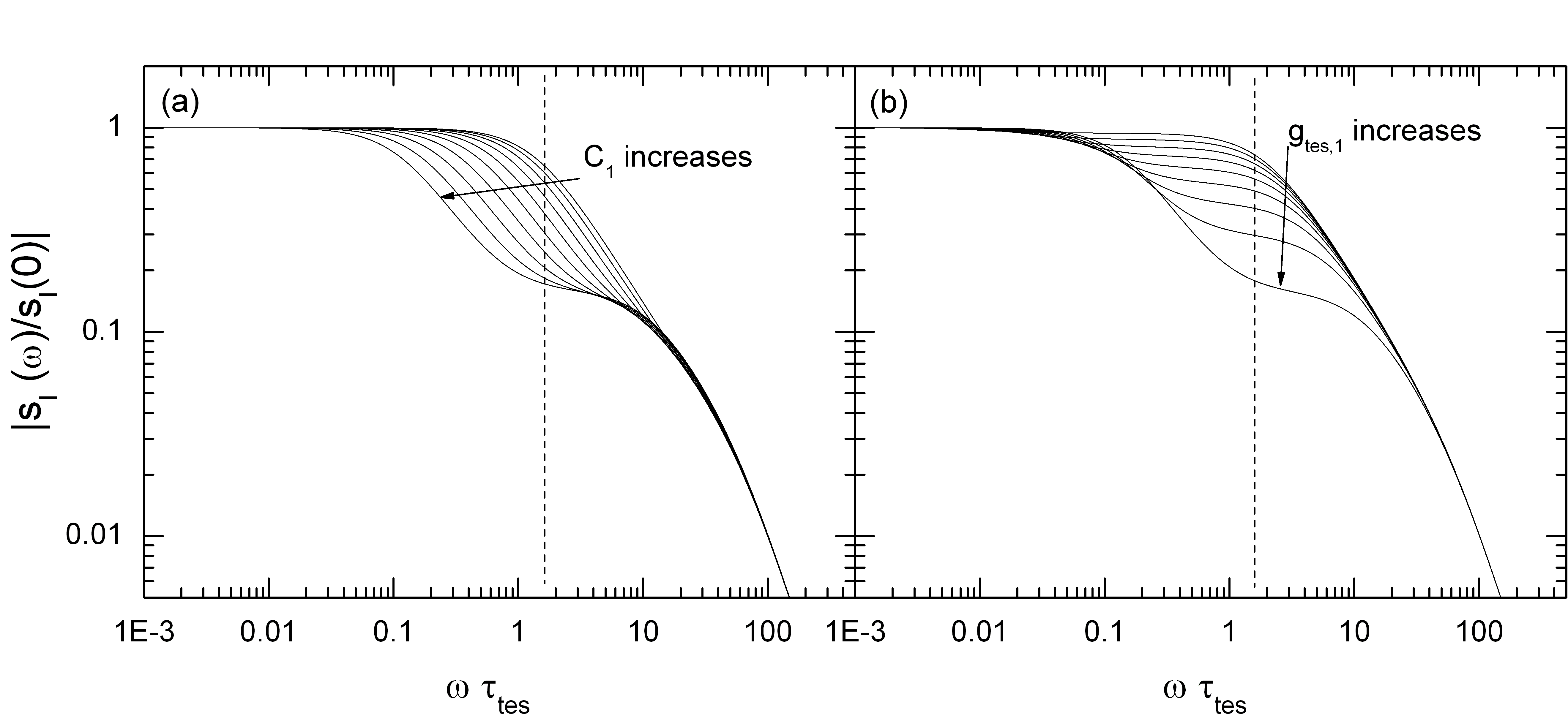
The effect of the loop gain on the current responsivity is well known, with higher loop gain increasing the responsivity at frequencies below the effective thermal time constant (where the responsivity starts to roll-off), and moving the time constant to higher frequencies. This takes place regardless of the complexity of the thermal model. On the other hand, the effect of changing C1subscript𝐶1C_{1} and gtes,1subscript𝑔𝑡𝑒𝑠1g_{tes,1} is not so self-evident. In Fig. 3, we plot how C1subscript𝐶1C_{1} and gtes,1subscript𝑔𝑡𝑒𝑠1g_{tes,1} in the two-block thermal circuits affect the responsivity, using the hanging model as an example (other models behave in a similar manner). We plot only the magnitude |sI(ω)|subscript𝑠𝐼𝜔|s_{I}(\omega)|, as the phase is irrelevant for noise considerations, which is the focus in this work. We see from the plots that for the usual case where the electrical cut-off frequency is above the thermal cut-off frequency (low enough inductance L𝐿L), the effect of the extra thermal block is to reduce the responsivity in the mid- frequency range starting from τ11superscriptsubscript𝜏11\tau_{1}^{-1}. Increasing C1subscript𝐶1C_{1} moves the first partial cut-off set by τ11superscriptsubscript𝜏11\tau_{1}^{-1} to lower frequencies [Fig. 3 (a)], whereas increasing gtes,1subscript𝑔𝑡𝑒𝑠1g_{tes,1} makes the intermediate frequency suppression stronger [Fig. 3 (b)].
Refer to caption
Figure 3: Responsivity of a two-block hanging model, with varying parameters. In both plots, we have used R0=0.1Ωsubscript𝑅00.1ΩR_{0}=0.1\mathrm{\Omega}, β=1𝛽1\beta=1, and τel=L/[RL+R0(1+β)]=0.015τtessubscript𝜏𝑒𝑙𝐿delimited-[]subscript𝑅𝐿subscript𝑅01𝛽0.015subscript𝜏𝑡𝑒𝑠\tau_{el}=L/[R_{L}+R_{0}(1+\beta)]=0.015\tau_{tes}, where τtes=Ctes/gtes,bsubscript𝜏𝑡𝑒𝑠subscript𝐶𝑡𝑒𝑠subscript𝑔𝑡𝑒𝑠𝑏\tau_{tes}=C_{tes}/g_{tes,b}. (a) |sI(ω)|subscript𝑠𝐼𝜔|s_{I}(\omega)| as a function of C1subscript𝐶1C_{1}, with C1/Ctes=0.33,0.49,0.73,1.1,1.65,2.48,3.71,5.57,8.35,12.5subscript𝐶1subscript𝐶𝑡𝑒𝑠0.330.490.731.11.652.483.715.578.3512.5C_{1}/C_{tes}=0.33,0.49,0.73,1.1,1.65,2.48,3.71,5.57,8.35,12.5, =1.651.65{\cal L}=1.65 and a=gtes,1/(gtes,1+gtes,b)=0.9𝑎subscript𝑔𝑡𝑒𝑠1subscript𝑔𝑡𝑒𝑠1subscript𝑔𝑡𝑒𝑠𝑏0.9a=g_{tes,1}/(g_{tes,1}+g_{tes,b})=0.9. Increasing C1subscript𝐶1C_{1} corresponds to a shift of the partial thermal cut-off to lower frequencies, and the development of a ”knee” in the intermediate frequency range. (b) |sI(ω)|subscript𝑠𝐼𝜔|s_{I}(\omega)| as a function of a𝑎a (or gtes,1subscript𝑔𝑡𝑒𝑠1g_{tes,1}), with a=0.1,0.2,0.3,0.4,0.5,0.6,0.7,0.8,0.9𝑎0.10.20.30.40.50.60.70.80.9a=0.1,0.2,0.3,0.4,0.5,0.6,0.7,0.8,0.9, =1.651.65{\cal L}=1.65 and C1/Ctes=10subscript𝐶1subscript𝐶𝑡𝑒𝑠10C_{1}/C_{tes}=10. Increasing a𝑎a corresponds to the decrease of responsivity in the intermediate frequency range. Dashed line shows the simple model effective thermal time constant.

II.4 Thermodynamic noise

In TES detectors, there are several possible mechanisms for noise. Some of them are directly associated with superconductivity such as phase-slip shot noise psn1 ; psn2 , fluctuation superconductivity noise fsn ; seidel and vortex motion noise vortex . In all these mechanisms, there are external parameters such as the material quality of the superconducting film or the magnetic field that affect the noise, and thus these superconductivity related noise sources can, in principle, be controlled to some extent. In addition, there is currently no conclusive evidence for a significant role of the superconducting noise sources being dominant in TES detectors. In this paper we therefore only concentrate on the two unavoidable noise sources in TES detectors: (i) thermodynamic fluctuations of heat within the thermal circuit (thermal fluctuation noise, TFN) mather1 , and (ii) electrical fluctuations of the resistive circuit elements (Johnson noise) mather1 ; johnson ; nyquist .

The thermal fluctuation noise and Johnson noise of a simple one-block bolometer were discussed long ago mather1 , and their effect on a TES detector in negative electrothermal feedback has been reviewed thoroughly in Ref. irwinbook . TFN and Johnson noise properties of some two- and three-body models have also been discussed in Refs. hoevers ; zink ; galeazzi ; takeinote ; zhaothesis , but none of those Refs. give very simple compact analytical formulas for noise, nor do they discuss all the models covered in this work. In this section, compact analytical results for the current noise are given for all three variations of the two block models (and in Sect. III for two three-block models), using the already derived results for the complex impedance and responsivity.

II.4.1 Hanging model

Thermal fluctuation noise

For each thermal conductance in the model, there are power fluctuations on top of the steady state power that is conducted. These fluctuations can be taken into account in a straightforward manner by adding appropriate fluctuation power terms δPi𝛿subscript𝑃𝑖\delta P_{i} into the constituting thermal equations in Eqs. 1, which for the hanging model then become (ignoring external power input)

CtesdTtesdtsubscript𝐶𝑡𝑒𝑠𝑑subscript𝑇𝑡𝑒𝑠𝑑𝑡\displaystyle C_{tes}\frac{dT_{tes}}{dt} =\displaystyle= PJA(TtesnT1n)δPtes,1B(TtesmTbm)δPtes,bsubscript𝑃𝐽𝐴superscriptsubscript𝑇𝑡𝑒𝑠𝑛superscriptsubscript𝑇1𝑛𝛿subscript𝑃𝑡𝑒𝑠1𝐵superscriptsubscript𝑇𝑡𝑒𝑠𝑚superscriptsubscript𝑇𝑏𝑚𝛿subscript𝑃𝑡𝑒𝑠𝑏\displaystyle P_{J}-A\left(T_{tes}^{n}-T_{1}^{n}\right)-\delta P_{tes,1}-B\left(T_{tes}^{m}-T_{b}^{m}\right)-\delta P_{tes,b}
C1dT1dtsubscript𝐶1𝑑subscript𝑇1𝑑𝑡\displaystyle C_{1}\frac{dT_{1}}{dt} =\displaystyle= A(TtesnT1n)+δPtes,1.𝐴superscriptsubscript𝑇𝑡𝑒𝑠𝑛superscriptsubscript𝑇1𝑛𝛿subscript𝑃𝑡𝑒𝑠1\displaystyle A\left(T_{tes}^{n}-T_{1}^{n}\right)+\delta P_{tes,1}. (16)

Note how the sign has to be different for the δPtes,1𝛿subscript𝑃𝑡𝑒𝑠1\delta P_{tes,1} terms in the two equations, because an increase in outflowing power from ij𝑖𝑗i\rightarrow j is equivalent with a decrease of the outflowing power from ji𝑗𝑖j\rightarrow i. Linearization and transformation into frequency domain, as before, thus lead to equations that resemble the equations for complex impedance and responsivity. After some algebra, one can write surprisingly simple results (disregarding correlations between the the two fluctuating sources) for the two TFN current noise spectral densities SI,i(ω)=|Iω|i2subscript𝑆𝐼𝑖𝜔superscriptsubscriptsubscript𝐼𝜔𝑖2S_{I,i}(\omega)=|I_{\omega}|_{i}^{2} associated with the two thermal links gisubscript𝑔𝑖g_{i}:

|Iω|tes,b2subscriptsuperscriptsubscript𝐼𝜔2𝑡𝑒𝑠𝑏\displaystyle|I_{\omega}|^{2}_{tes,b} =\displaystyle= Ptes,b2|Zcirc|2I02|ZtesR0(1+β)|2R02(2+β)2=Ptes,b2|sI(ω)|2,superscriptsubscript𝑃𝑡𝑒𝑠𝑏2superscriptsubscript𝑍𝑐𝑖𝑟𝑐2superscriptsubscript𝐼02superscriptsubscript𝑍𝑡𝑒𝑠subscript𝑅01𝛽2superscriptsubscript𝑅02superscript2𝛽2superscriptsubscript𝑃𝑡𝑒𝑠𝑏2superscriptsubscript𝑠𝐼𝜔2\displaystyle\frac{P_{tes,b}^{2}}{|Z_{circ}|^{2}I_{0}^{2}}\frac{|Z_{tes}-R_{0}(1+\beta)|^{2}}{R_{0}^{2}(2+\beta)^{2}}=P_{tes,b}^{2}|s_{I}(\omega)|^{2},
|Iω|tes,12subscriptsuperscriptsubscript𝐼𝜔2𝑡𝑒𝑠1\displaystyle|I_{\omega}|^{2}_{tes,1} =\displaystyle= Ptes,12|Zcirc|2I02|ZtesR0(1+β)|2R02(2+β)2ω2τ121+ω2τ12=Ptes,12|sI(ω)|2ω2τ121+ω2τ12,superscriptsubscript𝑃𝑡𝑒𝑠12superscriptsubscript𝑍𝑐𝑖𝑟𝑐2superscriptsubscript𝐼02superscriptsubscript𝑍𝑡𝑒𝑠subscript𝑅01𝛽2superscriptsubscript𝑅02superscript2𝛽2superscript𝜔2superscriptsubscript𝜏121superscript𝜔2superscriptsubscript𝜏12superscriptsubscript𝑃𝑡𝑒𝑠12superscriptsubscript𝑠𝐼𝜔2superscript𝜔2superscriptsubscript𝜏121superscript𝜔2superscriptsubscript𝜏12\displaystyle\frac{P_{tes,1}^{2}}{|Z_{circ}|^{2}I_{0}^{2}}\frac{|Z_{tes}-R_{0}(1+\beta)|^{2}}{R_{0}^{2}(2+\beta)^{2}}\frac{\omega^{2}\tau_{1}^{2}}{1+\omega^{2}\tau_{1}^{2}}=P_{tes,1}^{2}|s_{I}(\omega)|^{2}\frac{\omega^{2}\tau_{1}^{2}}{1+\omega^{2}\tau_{1}^{2}}, (17)

where we have defined the power TFN spectral densities of the two thermal links as Ptes,b2superscriptsubscript𝑃𝑡𝑒𝑠𝑏2P_{tes,b}^{2} and Ptes,12superscriptsubscript𝑃𝑡𝑒𝑠12P_{tes,1}^{2}, and the total TFN current noise spectral density is simply the sum of the above two components SI,TFN(ω)=|Iω|tes,b2+|Iω|tes,12subscript𝑆𝐼𝑇𝐹𝑁𝜔subscriptsuperscriptsubscript𝐼𝜔2𝑡𝑒𝑠𝑏subscriptsuperscriptsubscript𝐼𝜔2𝑡𝑒𝑠1S_{I,TFN}(\omega)=|I_{\omega}|^{2}_{tes,b}+|I_{\omega}|^{2}_{tes,1}. The exact form of TFN power spectral densities Pi2superscriptsubscript𝑃𝑖2P_{i}^{2} depend on the details of the nature of the thermal links, and results have been derived for phonon transport in the fully ballistic or 1-D diffusive limits, as reviewed in Ref. mccammonbook , or for electron-phonon or Kapitza thermal conductance kuzminJAP ; dragos . For all cases where the temperature difference between two adjoining heat capacity blocks is a step function (ballistic phonons, e-p interaction, Kapitza resistance), the TFN power spectral density is well approximated by

Pi,j2=2kB(gi,j(Ti)Ti2+gi,j(Tj)Tj2).superscriptsubscript𝑃𝑖𝑗22subscript𝑘𝐵subscript𝑔𝑖𝑗subscript𝑇𝑖superscriptsubscript𝑇𝑖2subscript𝑔𝑖𝑗subscript𝑇𝑗superscriptsubscript𝑇𝑗2P_{i,j}^{2}=2k_{B}(g_{i,j}(T_{i})T_{i}^{2}+g_{i,j}(T_{j})T_{j}^{2}). (18)

Looking at Eqs. 17, we see that the first term is the usual TFN noise term (”phonon noise”) that exists in the one-block circuit, as well. Its frequency dependence is now simply complicated by the more complex responsivity, and the |Iω|tes,b2subscriptsuperscriptsubscript𝐼𝜔2𝑡𝑒𝑠𝑏|I_{\omega}|^{2}_{tes,b} noise spectra would look just like the responsivity plots in Fig. 3. On the other hand, the second, new noise term looks very different: It has significant weight only above the frequencies set by the time constant of the extra heat capacity τ1subscript𝜏1\tau_{1}.

Johnson noise of the TES

The Johnson noise of the TES has a slightly more complex influence on the thermal and electrical equations: the noise is electrical in origin, so there is a fluctuation term in the electrical part of the constituent equations. In addition, the dissipated bias power also fluctuates, affecting the thermal part of the circuit. One way to properly take both effects into account was discussed in Ref. irwinbook , by introducing the so called internal impedance matrix. We follow the same approach, which leads to a different Taylor expansion of the Joule power (only in terms of current), and to a expression in frequency domain PJ=I0[(R0RL)iωL]Iωsubscript𝑃𝐽subscript𝐼0delimited-[]subscript𝑅0subscript𝑅𝐿𝑖𝜔𝐿subscript𝐼𝜔P_{J}=I_{0}[(R_{0}-R_{L})-i\omega L]I_{\omega}, if the simplest bias circuit is assumed. That leads to a set of equations in frequency space

iωTω,tes𝑖𝜔subscript𝑇𝜔𝑡𝑒𝑠\displaystyle i\omega T_{\omega,tes} =\displaystyle= (R0RLiωL)I0CtesIω1τI(1H)Tω,tes+1τtes,1Tω,1subscript𝑅0subscript𝑅𝐿𝑖𝜔𝐿subscript𝐼0subscript𝐶𝑡𝑒𝑠subscript𝐼𝜔1subscript𝜏𝐼1subscript𝐻subscript𝑇𝜔𝑡𝑒𝑠1subscript𝜏𝑡𝑒𝑠1subscript𝑇𝜔1\displaystyle\frac{(R_{0}-R_{L}-i\omega L)I_{0}}{C_{tes}}I_{\omega}-\frac{1}{\tau_{I}(1-{\cal L}_{H})}T_{\omega,tes}+\frac{1}{\tau_{tes,1}}T_{\omega,1}
iωTω,1𝑖𝜔subscript𝑇𝜔1\displaystyle i\omega T_{\omega,1} =\displaystyle= 1τ1(Tω,tesTω,1)1subscript𝜏1subscript𝑇𝜔𝑡𝑒𝑠subscript𝑇𝜔1\displaystyle\frac{1}{\tau_{1}}\left(T_{\omega,tes}-T_{\omega,1}\right)
iωLIω𝑖𝜔𝐿subscript𝐼𝜔\displaystyle i\omega LI_{\omega} =\displaystyle= Vω,tes[RL+R0(1+β)]IωH(gtes,1+gtes,b)I0Tω,tes,subscript𝑉𝜔𝑡𝑒𝑠delimited-[]subscript𝑅𝐿subscript𝑅01𝛽subscript𝐼𝜔subscript𝐻subscript𝑔𝑡𝑒𝑠1subscript𝑔𝑡𝑒𝑠𝑏subscript𝐼0subscript𝑇𝜔𝑡𝑒𝑠\displaystyle V_{\omega,tes}-\left[R_{L}+R_{0}(1+\beta)\right]I_{\omega}-\frac{{\cal L}_{H}(g_{tes,1}+g_{tes,b})}{I_{0}}T_{\omega,tes}, (19)

with the notation the same as for Eqs. 4, and where Vω,tessubscript𝑉𝜔𝑡𝑒𝑠V_{\omega,tes} is the Johnson voltage noise of the TES, which in equilibrium has the well known expression Vω,tes=4kBT0R0subscript𝑉𝜔𝑡𝑒𝑠4subscript𝑘𝐵subscript𝑇0subscript𝑅0V_{\omega,tes}=\sqrt{4k_{B}T_{0}R_{0}}, but which has been shown irwinnoise to depend on the parameter β𝛽\beta in the first order as Vω,tes=4kBT0R0(1+2β)subscript𝑉𝜔𝑡𝑒𝑠4subscript𝑘𝐵subscript𝑇0subscript𝑅012𝛽V_{\omega,tes}=\sqrt{4k_{B}T_{0}R_{0}(1+2\beta)}.

After algebra, one gets an expression for the Johnson current noise spectral density SI,J(ω)=|Iω|J2subscript𝑆𝐼𝐽𝜔subscriptsuperscriptsubscript𝐼𝜔2𝐽S_{I,J}(\omega)=|I_{\omega}|^{2}_{J}, which is expressed in terms of the known TES complex impedance as

|Iω|J2=Vω,tes2R02(2+β)2|Ztes+R0Zcirc|2,subscriptsuperscriptsubscript𝐼𝜔2𝐽superscriptsubscript𝑉𝜔𝑡𝑒𝑠2superscriptsubscript𝑅02superscript2𝛽2superscriptsubscript𝑍𝑡𝑒𝑠subscript𝑅0subscript𝑍𝑐𝑖𝑟𝑐2|I_{\omega}|^{2}_{J}=\frac{V_{\omega,tes}^{2}}{R_{0}^{2}(2+\beta)^{2}}\left|\frac{Z_{tes}+R_{0}}{Z_{circ}}\right|^{2}, (20)

where we have again used the definition of the circuit impedance Zcirc=Ztes+RL+iωLsubscript𝑍𝑐𝑖𝑟𝑐subscript𝑍𝑡𝑒𝑠subscript𝑅𝐿𝑖𝜔𝐿Z_{circ}=Z_{tes}+R_{L}+i\omega L. This noise adds in quadrature to the TFN noise terms, as it is uncorrelated with them.

Johnson noise of the Thevenin (shunt) resistor, or other external voltage noise

The Johnson noise due to the shunt and parasitic resistances (RLsubscript𝑅𝐿R_{L}) does not influence the thermal circuit, and is simply

|Iω|sh2=Vω,sh2|Zcirc|2,subscriptsuperscriptsubscript𝐼𝜔2𝑠superscriptsubscript𝑉𝜔𝑠2superscriptsubscript𝑍𝑐𝑖𝑟𝑐2|I_{\omega}|^{2}_{sh}=\frac{V_{\omega,sh}^{2}}{|Z_{circ}|^{2}}, (21)

where Zcirc=Ztes+RL+iωLsubscript𝑍𝑐𝑖𝑟𝑐subscript𝑍𝑡𝑒𝑠subscript𝑅𝐿𝑖𝜔𝐿Z_{circ}=Z_{tes}+R_{L}+i\omega L is the full circuit impedance and

Vω,sh2=4kBTshRL,superscriptsubscript𝑉𝜔𝑠24subscript𝑘𝐵subscript𝑇𝑠subscript𝑅𝐿V_{\omega,sh}^{2}=4k_{B}T_{sh}R_{L}, (22)

if all of RLsubscript𝑅𝐿R_{L} is at temperature Tshsubscript𝑇𝑠T_{sh}. If RLsubscript𝑅𝐿R_{L} consists of two parts, say shunt resistance Rshsubscript𝑅𝑠R_{sh} and parasitic resistance irwinbook Rparasubscript𝑅𝑝𝑎𝑟𝑎R_{para}, and those two parts are at different temperatures Tshsubscript𝑇𝑠T_{sh} and Tparasubscript𝑇𝑝𝑎𝑟𝑎T_{para}, then more accurately Vω,sh2=4kB(TshRsh+TparaRpara)superscriptsubscript𝑉𝜔𝑠24subscript𝑘𝐵subscript𝑇𝑠subscript𝑅𝑠subscript𝑇𝑝𝑎𝑟𝑎subscript𝑅𝑝𝑎𝑟𝑎V_{\omega,sh}^{2}=4k_{B}(T_{sh}R_{sh}+T_{para}R_{para}). Any other external voltage noise would also contribute through Eq. 21, but with Vω,shsubscript𝑉𝜔𝑠V_{\omega,sh} given by the external voltage noise amplitude.

Noise plots

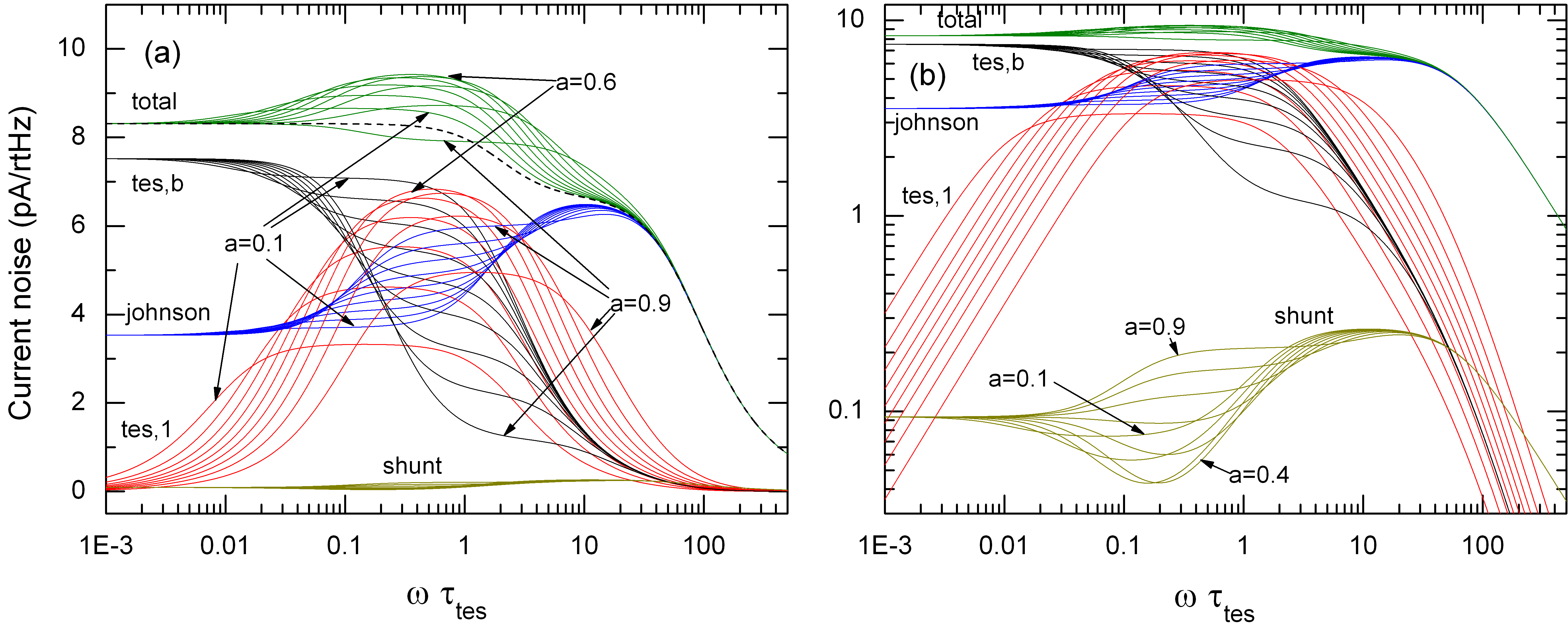
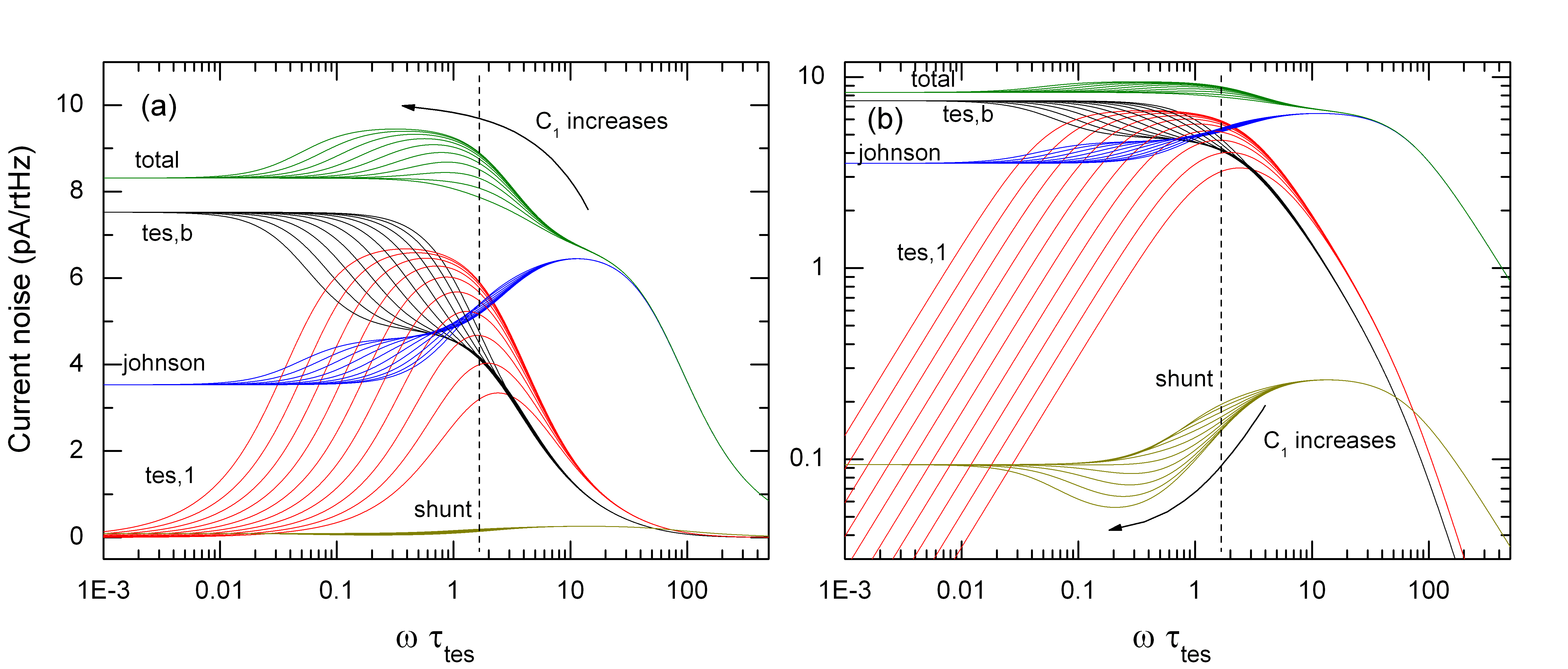
To gain some intuition on the noise, we plot here some examples how the different TES current noise components vary with the thermal parameters. In Fig. 4, we first show how noise depends on C1subscript𝐶1C_{1}. When C1/Ctessubscript𝐶1subscript𝐶𝑡𝑒𝑠C_{1}/C_{tes} is greater than 0.5absent0.5\approx 0.5, a clear bump in the noise spectrum develops in the mid-frequency range between 1/τ11subscript𝜏11/\tau_{1} and the effective thermal cut-off set by Ctessubscript𝐶𝑡𝑒𝑠C_{tes}. The onset of the bump moves to lower frequencies with increasing C1subscript𝐶1C_{1}, and it is, for the used ratio of thermal conductances a=gtes,1/(gtes,1+gtes,b)=0.5𝑎subscript𝑔𝑡𝑒𝑠1subscript𝑔𝑡𝑒𝑠1subscript𝑔𝑡𝑒𝑠𝑏0.5a=g_{tes,1}/(g_{tes,1}+g_{tes,b})=0.5, dominated by the thermal fluctuation noise component of the hanging block |Iω|tes,1subscriptsubscript𝐼𝜔𝑡𝑒𝑠1|I_{\omega}|_{tes,1}, as the phonon noise |Iω|tes,bsubscriptsubscript𝐼𝜔𝑡𝑒𝑠𝑏|I_{\omega}|_{tes,b} actually decreases in the mid-frequency range. The magnitude of the bump saturates to a value determined by the thermal conductance gtes,1subscript𝑔𝑡𝑒𝑠1g_{tes,1} when C1subscript𝐶1C_{1} is large enough. Johnson noise also develops a minor step feature, and although small in Fig. 4, its relative strength compared to the TFN noise depends on the details, such as the value of loop gain and resistance. The shunt resistor noise actually develops a dip for the values of {\cal L} and a𝑎a used in Fig. 4, but for the parameter values used here, its magnitude is small.
Refer to caption
Figure 4: (Color online) Current noise of a two-block hanging model, with varying C1/Ctes=0.33,0.49,0.73,1.1,1.65,2.48,3.71,5.57,8.35,12.5subscript𝐶1subscript𝐶𝑡𝑒𝑠0.330.490.731.11.652.483.715.578.3512.5C_{1}/C_{tes}=0.33,0.49,0.73,1.1,1.65,2.48,3.71,5.57,8.35,12.5 in linear-log (a) and log-log (b) scales. Increasing C1subscript𝐶1C_{1} corresponds to a shift of the onset of the bump (or dip in |Iω|tes,bsubscriptsubscript𝐼𝜔𝑡𝑒𝑠𝑏|I_{\omega}|_{tes,b} and |Iω|shsubscriptsubscript𝐼𝜔𝑠|I_{\omega}|_{sh}) to lower frequencies, and an increase of the magnitude of |Iω|tes,1subscriptsubscript𝐼𝜔𝑡𝑒𝑠1|I_{\omega}|_{tes,1} noise component. Other parameters: =1.651.65{\cal L}=1.65, a=gtes,1/(gtes,1+gtes,b)=0.5𝑎subscript𝑔𝑡𝑒𝑠1subscript𝑔𝑡𝑒𝑠1subscript𝑔𝑡𝑒𝑠𝑏0.5a=g_{tes,1}/(g_{tes,1}+g_{tes,b})=0.5, R0=0.1Ωsubscript𝑅00.1ΩR_{0}=0.1\mathrm{\Omega}, β=1𝛽1\beta=1, RL=0.001Ωsubscript𝑅𝐿0.001ΩR_{L}=0.001\mathrm{\Omega}, I0=10μsubscript𝐼010𝜇I_{0}=10\muA, gtes,b=1subscript𝑔𝑡𝑒𝑠𝑏1g_{tes,b}=1 nW/K, τel=L/[RL+R0(1+β)]=0.015τtessubscript𝜏𝑒𝑙𝐿delimited-[]subscript𝑅𝐿subscript𝑅01𝛽0.015subscript𝜏𝑡𝑒𝑠\tau_{el}=L/[R_{L}+R_{0}(1+\beta)]=0.015\tau_{tes}, τtes=Ctes/gtes,bsubscript𝜏𝑡𝑒𝑠subscript𝐶𝑡𝑒𝑠subscript𝑔𝑡𝑒𝑠𝑏\tau_{tes}=C_{tes}/g_{tes,b}. Dashed line shows the simple model effective thermal time constant.

In Fig. 5, the effect of the value of the hanging thermal conductance gtes,1subscript𝑔𝑡𝑒𝑠1g_{tes,1} is studied, by plotting the noise spectra as a function of the varying relative strength a=gtes,1/(gtes,1+gtes,b)𝑎subscript𝑔𝑡𝑒𝑠1subscript𝑔𝑡𝑒𝑠1subscript𝑔𝑡𝑒𝑠𝑏a=g_{tes,1}/(g_{tes,1}+g_{tes,b}). The difference to the effect of C1subscript𝐶1C_{1} is that instead of developing a bump with constant magnitude, the bump magnitude evolves with a𝑎a in a non-monotonous manner, having a maximum at around a0.6𝑎0.6a\approx 0.6. In addition, the bump shifts up in frequency with increasing a𝑎a (both low and high frequency sides). In other words, the effect of the hanging block on noise is largest for approximately equal magnitudes of the two thermal conductances, just like for the complex impedance. Interestingly, the bump in total noise eventually develops into a step-down feature for the highest values of a𝑎a here (a=0.9𝑎0.9a=0.9), where in a certain region of frequencies the noise can be lower than the simple model noise. This does not imply, however, that the noise equivalent power NEP=|Iω|tot/|sI(ω)|𝑁𝐸𝑃subscriptsubscript𝐼𝜔𝑡𝑜𝑡subscript𝑠𝐼𝜔NEP=|I_{\omega}|_{tot}/|s_{I}(\omega)| is lower, because the responsivity is reduced even more than noise in that frequency region (See Fig. 3). Looking at the different components of the noise, one sees that the non-monotonous behavior in total noise is caused by the hanging block TFN noise |Iω|tes,1subscriptsubscript𝐼𝜔𝑡𝑒𝑠1|I_{\omega}|_{tes,1}, whereas the phonon noise |Iω|tes,bsubscriptsubscript𝐼𝜔𝑡𝑒𝑠𝑏|I_{\omega}|_{tes,b} (Johnson noise) decreases (increases) monotonously in mid-frequency range with a𝑎a. The dip in shunt noise in the mid-frequency range is deepest at a0.4𝑎0.4a\approx 0.4, and becomes a step-up feature for a>0.6𝑎0.6a>0.6.

Refer to caption
Figure 5: Current noise of a two-block hanging model, with varying a=gtes,1/(gtes,1+gtes,b)=0.1,0.2,0.3,0.4,0.5,0.6,0.7,0.8,0.9formulae-sequence𝑎subscript𝑔𝑡𝑒𝑠1subscript𝑔𝑡𝑒𝑠1subscript𝑔𝑡𝑒𝑠𝑏0.10.20.30.40.50.60.70.80.9a=g_{tes,1}/(g_{tes,1}+g_{tes,b})=0.1,0.2,0.3,0.4,0.5,0.6,0.7,0.8,0.9 in linear-log (a) and log-log (b) scales. Increasing a𝑎a corresponds to a shift of all the extra features to higher frequencies (both low- and high-frequency sides), a decrease of the phonon noise |Iω|tes,bsubscriptsubscript𝐼𝜔𝑡𝑒𝑠𝑏|I_{\omega}|_{tes,b} and an increase of the Johnson noise |Iω|Jsubscriptsubscript𝐼𝜔𝐽|I_{\omega}|_{J} in the mid-frequency range, and a non-monotonous behavior of |Iω|tes,1subscriptsubscript𝐼𝜔𝑡𝑒𝑠1|I_{\omega}|_{tes,1} and |Iω|shsubscriptsubscript𝐼𝜔𝑠|I_{\omega}|_{sh}. The magnitude of |Iω|tes,1subscriptsubscript𝐼𝜔𝑡𝑒𝑠1|I_{\omega}|_{tes,1} noise component and the total noise have a maximum at around a=0.6𝑎0.6a=0.6, and |Iω|shsubscriptsubscript𝐼𝜔𝑠|I_{\omega}|_{sh} a minimum around a=0.4𝑎0.4a=0.4. Other parameters: =1.651.65{\cal L}=1.65, C1/Ctes=10subscript𝐶1subscript𝐶𝑡𝑒𝑠10C_{1}/C_{tes}=10, R0=0.1Ωsubscript𝑅00.1ΩR_{0}=0.1\mathrm{\Omega}, β=1𝛽1\beta=1, RL=0.001Ωsubscript𝑅𝐿0.001ΩR_{L}=0.001\mathrm{\Omega}, I0=10μsubscript𝐼010𝜇I_{0}=10\muA, gtes,b=1subscript𝑔𝑡𝑒𝑠𝑏1g_{tes,b}=1 nW/K, τel=L/[RL+R0(1+β)]=0.015τtessubscript𝜏𝑒𝑙𝐿delimited-[]subscript𝑅𝐿subscript𝑅01𝛽0.015subscript𝜏𝑡𝑒𝑠\tau_{el}=L/[R_{L}+R_{0}(1+\beta)]=0.015\tau_{tes}, τtes=Ctes/gtes,bsubscript𝜏𝑡𝑒𝑠subscript𝐶𝑡𝑒𝑠subscript𝑔𝑡𝑒𝑠𝑏\tau_{tes}=C_{tes}/g_{tes,b}. Dashed line in (a) shows the single-block (no C1subscript𝐶1C_{1}) result for total noise.

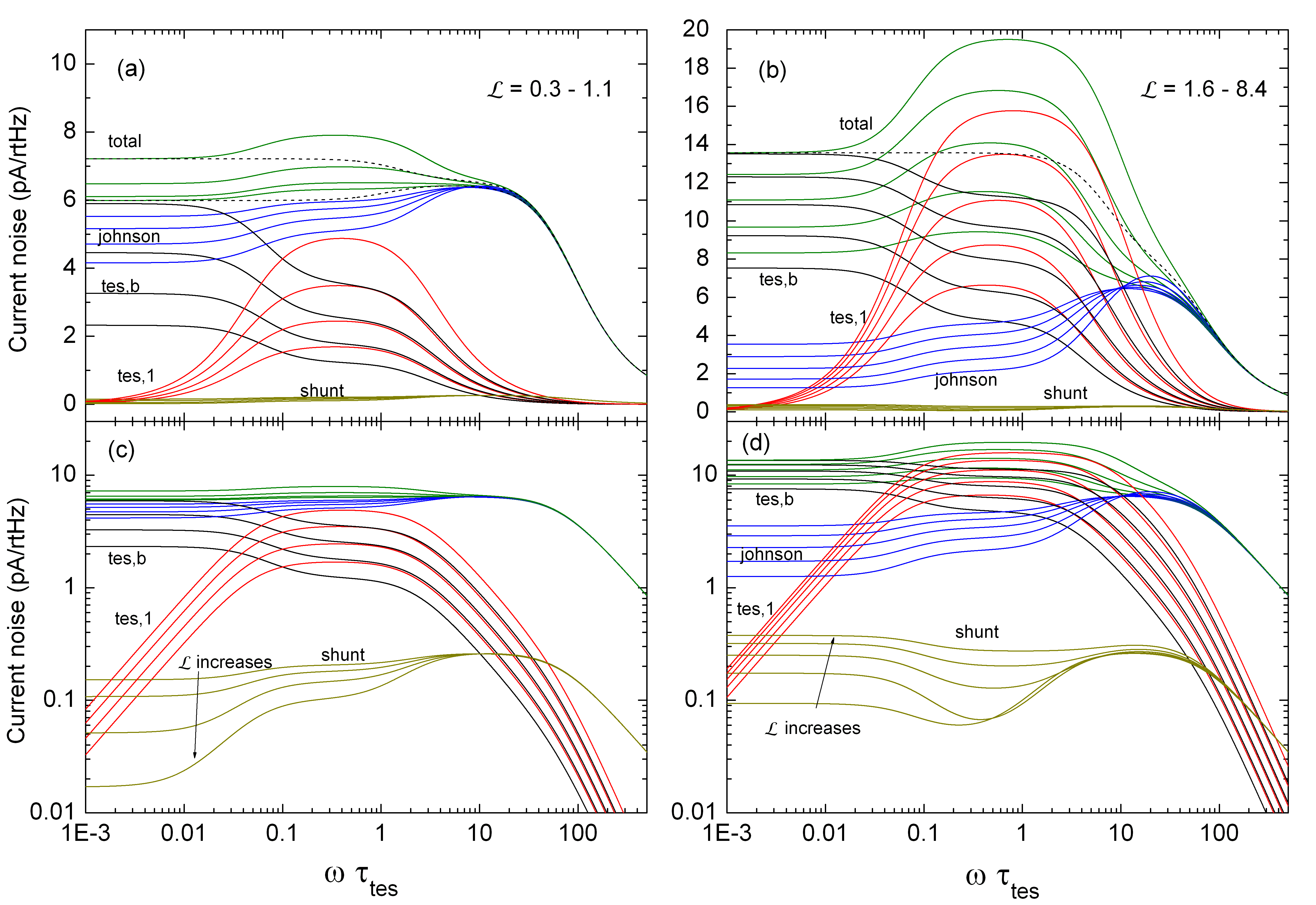
Finally, we also want to plot the dependence on the loop gain {\cal L}, shown in Fig. 6. The main effect of increasing {\cal L} is the same as in the simple model irwinbook , which is that it increases the magnitude of the thermal noise components, and reduces the Johnson noise level below the frequencies set by the effective thermal time constant. This means that for low values of <11{\cal L}<1 the total noise is Johnson noise limited [Figs 6 (a) and (c)], whereas for higher loop gains >11{\cal L}>1 the thermal noise dominates [Figs 6 (b) and (d)]. This transition means that the relative size of the mid-frequency bump first grows faster with {\cal L}, and then more slowly when Johnson noise becomes irrelevant. Notice that for high {\cal L}, also the high frequency cut-off for the thermal noise components moves to higher frequencies, due to the increase of the effective thermal time constant. The shunt noise behaves, again, in a more complex way. For low <11{\cal L}<1, the low-frequency part of it is first suppressed like Johnson noise, but for high >11{\cal L}>1 the situation reverses, and eventually for the highest values, the low-frequency shunt noise is above the high-frequency level.
Refer to caption
Figure 6: (Color online) Current noise of a two-block hanging model, with varying {\cal L}. In the left panels =0.33,0.49,0.73,1.10.330.490.731.1{\cal L}=0.33,0.49,0.73,1.1 in linear-log (a) and log-log (c) scales, whereas in the right panels =1.65,2.48,3.71,5.57,8.351.652.483.715.578.35{\cal L}=1.65,2.48,3.71,5.57,8.35, in linear-log (b) and log-log (d) scales. Increasing {\cal L} corresponds to an increase of the |Iω|tes,bsubscriptsubscript𝐼𝜔𝑡𝑒𝑠𝑏|I_{\omega}|_{tes,b} and |Iω|tes,1subscriptsubscript𝐼𝜔𝑡𝑒𝑠1|I_{\omega}|_{tes,1} TFN noise levels, and an increase of the thermal cut-off frequency for >11{\cal L}>1. The low-frequency Johnson noise |Iω|Jsubscriptsubscript𝐼𝜔𝐽|I_{\omega}|_{J} decreases, and |Iω|shsubscriptsubscript𝐼𝜔𝑠|I_{\omega}|_{sh} behaves non-monotonously. The minimum of the low-frequency |Iω|shsubscriptsubscript𝐼𝜔𝑠|I_{\omega}|_{sh} noise component appears at 11{\cal L}\approx 1. Other parameters: a=0.5𝑎0.5a=0.5, C1/Ctes=10subscript𝐶1subscript𝐶𝑡𝑒𝑠10C_{1}/C_{tes}=10, R0=0.1Ωsubscript𝑅00.1ΩR_{0}=0.1\mathrm{\Omega}, β=1𝛽1\beta=1, RL=0.001Ωsubscript𝑅𝐿0.001ΩR_{L}=0.001\mathrm{\Omega}, I0=10μsubscript𝐼010𝜇I_{0}=10\muA, gtes,b=1subscript𝑔𝑡𝑒𝑠𝑏1g_{tes,b}=1 nW/K, τel=L/[RL+R0(1+β)]=0.015τtessubscript𝜏𝑒𝑙𝐿delimited-[]subscript𝑅𝐿subscript𝑅01𝛽0.015subscript𝜏𝑡𝑒𝑠\tau_{el}=L/[R_{L}+R_{0}(1+\beta)]=0.015\tau_{tes}, τtes=Ctes/gtes,bsubscript𝜏𝑡𝑒𝑠subscript𝐶𝑡𝑒𝑠subscript𝑔𝑡𝑒𝑠𝑏\tau_{tes}=C_{tes}/g_{tes,b}. Dashed lines in (a) and (b) show a few results for the the one-block model for total noise.

II.4.2 Intermediate model

For the intermediate model, equivalent equations to Eqs. 16 can be written and solved in frequency domain, with the following simple results for the two TFN noise components:

|Iω|1,b2subscriptsuperscriptsubscript𝐼𝜔21𝑏\displaystyle|I_{\omega}|^{2}_{1,b} =\displaystyle= P1,b2|sI(ω)|2gtes,12(T1)(gtes,1(T1)+g1,b)211+ω2τ12,superscriptsubscript𝑃1𝑏2superscriptsubscript𝑠𝐼𝜔2superscriptsubscript𝑔𝑡𝑒𝑠12subscript𝑇1superscriptsubscript𝑔𝑡𝑒𝑠1subscript𝑇1subscript𝑔1𝑏211superscript𝜔2superscriptsubscript𝜏12\displaystyle P_{1,b}^{2}|s_{I}(\omega)|^{2}\frac{g_{tes,1}^{2}(T_{1})}{(g_{tes,1}(T_{1})+g_{1,b})^{2}}\frac{1}{1+\omega^{2}\tau_{1}^{2}},
|Iω|tes,12subscriptsuperscriptsubscript𝐼𝜔2𝑡𝑒𝑠1\displaystyle|I_{\omega}|^{2}_{tes,1} =\displaystyle= Ptes,12|sI(ω)|2g1,b2/(gtes,1(T1)+g1,b)2+ω2τ121+ω2τ12,superscriptsubscript𝑃𝑡𝑒𝑠12superscriptsubscript𝑠𝐼𝜔2superscriptsubscript𝑔1𝑏2superscriptsubscript𝑔𝑡𝑒𝑠1subscript𝑇1subscript𝑔1𝑏2superscript𝜔2superscriptsubscript𝜏121superscript𝜔2superscriptsubscript𝜏12\displaystyle P_{tes,1}^{2}|s_{I}(\omega)|^{2}\frac{g_{1,b}^{2}/(g_{tes,1}(T_{1})+g_{1,b})^{2}+\omega^{2}\tau_{1}^{2}}{1+\omega^{2}\tau_{1}^{2}}, (23)

where τ1=C1/(gtes,1(T1)+g1,b)subscript𝜏1subscript𝐶1subscript𝑔𝑡𝑒𝑠1subscript𝑇1subscript𝑔1𝑏\tau_{1}=C_{1}/(g_{tes,1}(T_{1})+g_{1,b}), as before for the intermediate model. The Johnson noise results (both TES ans shunt) have no direct dependence on the thermal model parameters, thus Equations 20 and 21 remain the same, as long as one uses the correct equation for Ztessubscript𝑍𝑡𝑒𝑠Z_{tes}. As Ztessubscript𝑍𝑡𝑒𝑠Z_{tes} does not qualitatively differ between the intermediate and hanging models, the Johnson noise terms also behave qualitatively the same way.
Refer to caption
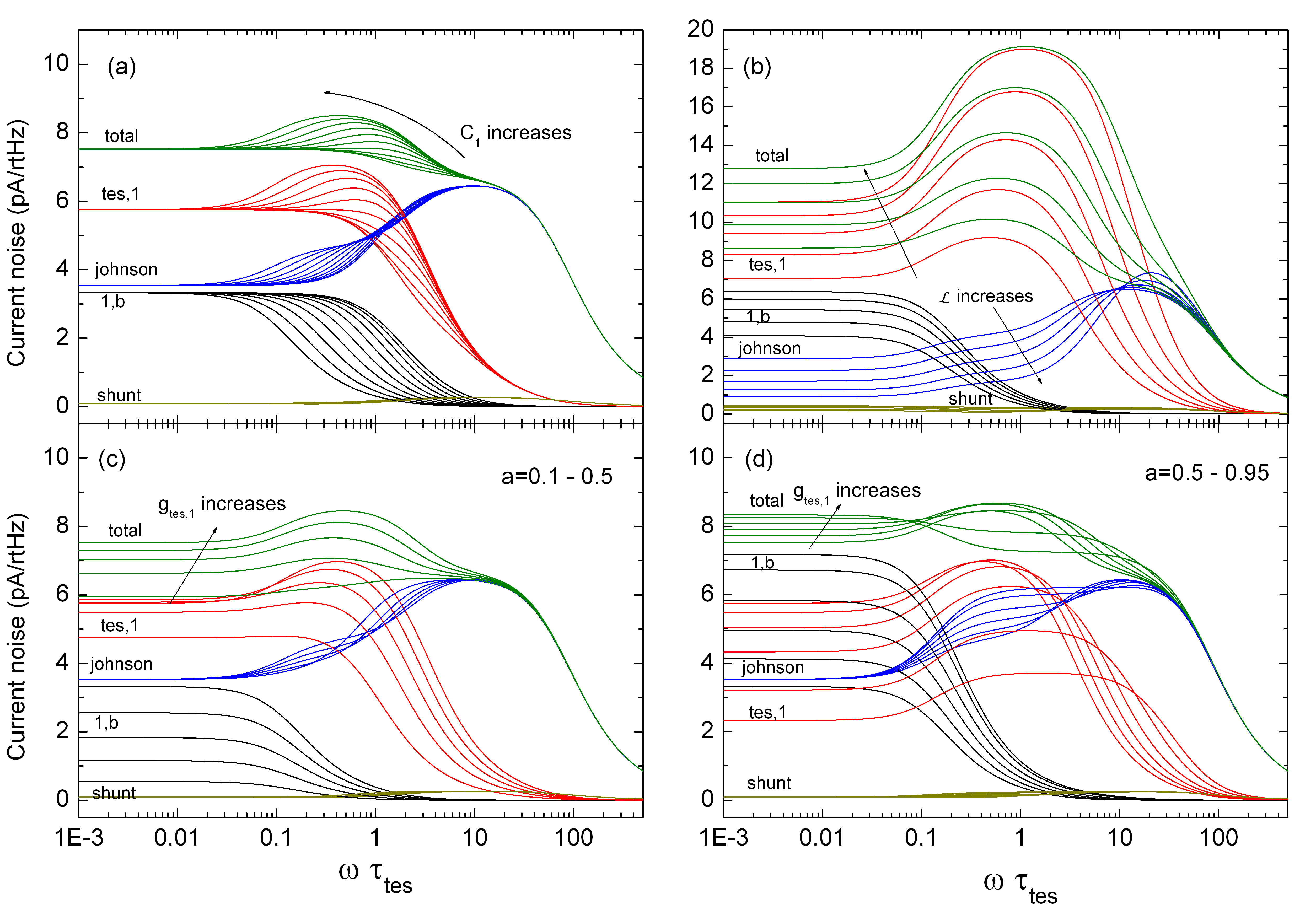
Figure 7: (Color online) (a) Current noise of a two-block intermediate model, with varying C1/Ctes=0.33,0.49,0.73,1.1,1.65,2.48,3.71,5.57,8.35,12.5subscript𝐶1subscript𝐶𝑡𝑒𝑠0.330.490.731.11.652.483.715.578.3512.5C_{1}/C_{tes}=0.33,0.49,0.73,1.1,1.65,2.48,3.71,5.57,8.35,12.5 in linear-log scale. Increasing C1subscript𝐶1C_{1} corresponds to a growth of the bump and a shift of its onset to lower frequencies, and a decrease of the cut-off frequency for the |Iω|1,bsubscriptsubscript𝐼𝜔1𝑏|I_{\omega}|_{1,b} noise component. (b) Same, with varying =2.48,3.71,5.57,8.35,12.52.483.715.578.3512.5{\cal L}=2.48,3.71,5.57,8.35,12.5. Increasing {\cal L} corresponds to an increase of the |Iω|1,bsubscriptsubscript𝐼𝜔1𝑏|I_{\omega}|_{1,b} and |Iω|tes,1subscriptsubscript𝐼𝜔𝑡𝑒𝑠1|I_{\omega}|_{tes,1} noise levels, and an increase of the thermal cut-off frequency for |Iω|tes,1subscriptsubscript𝐼𝜔𝑡𝑒𝑠1|I_{\omega}|_{tes,1}. (c) Same, with varying a=gtes,1(T1)/(gtes,1(T1)+g1,b)=0.1,0.2,0.3,0.4,0.5formulae-sequence𝑎subscript𝑔𝑡𝑒𝑠1subscript𝑇1subscript𝑔𝑡𝑒𝑠1subscript𝑇1subscript𝑔1𝑏0.10.20.30.40.5a=g_{tes,1}(T_{1})/(g_{tes,1}(T_{1})+g_{1,b})=0.1,0.2,0.3,0.4,0.5, and (d) with a=0.5,0.6,0.7,0.8,0.9,0.95𝑎0.50.60.70.80.90.95a=0.5,0.6,0.7,0.8,0.9,0.95. Increasing a𝑎a corresponds to a monotonous increase of the phonon noise level |Iω|1,bsubscriptsubscript𝐼𝜔1𝑏|I_{\omega}|_{1,b}, but a non-monotonous behavior of |Iω|tes,1subscriptsubscript𝐼𝜔𝑡𝑒𝑠1|I_{\omega}|_{tes,1} [first increase in (c), then decrease in (d)] with maximum bump amplitude around a=0.6𝑎0.6a=0.6 (maximum low-frequency noise around a=0.4𝑎0.4a=0.4), and a shift of the bump to higher frequencies. Johnson noise |Iω|Jsubscriptsubscript𝐼𝜔𝐽|I_{\omega}|_{J} increases in the mid-frequency range. Other parameters in plots (if not varied): =1.651.65{\cal L}=1.65, C1/Ctes=10subscript𝐶1subscript𝐶𝑡𝑒𝑠10C_{1}/C_{tes}=10, a=0.5𝑎0.5a=0.5, R0=0.1Ωsubscript𝑅00.1ΩR_{0}=0.1\mathrm{\Omega}, β=1𝛽1\beta=1, RL=0.001Ωsubscript𝑅𝐿0.001ΩR_{L}=0.001\mathrm{\Omega}, I0=10μsubscript𝐼010𝜇I_{0}=10\muA, g1,b=1subscript𝑔1𝑏1g_{1,b}=1 nW/K, τel=L/[RL+R0(1+β)]=0.015τtessubscript𝜏𝑒𝑙𝐿delimited-[]subscript𝑅𝐿subscript𝑅01𝛽0.015subscript𝜏𝑡𝑒𝑠\tau_{el}=L/[R_{L}+R_{0}(1+\beta)]=0.015\tau_{tes}, τtes=Ctes/g1,bsubscript𝜏𝑡𝑒𝑠subscript𝐶𝑡𝑒𝑠subscript𝑔1𝑏\tau_{tes}=C_{tes}/g_{1,b}.

In Fig. 7 we plot examples of how the noise depends on the most relevant parameters for this model. T1subscript𝑇1T_{1} was calculated using the simplifying assumption n=m=4𝑛𝑚4n=m=4. The results for the total noise as a function of C1subscript𝐶1C_{1} [Fig. 7 (a)] look nearly identical to the results of the hanging model, Fig. 4. The only main difference is that the level of low-frequency noise is lower because the intermediate block is at a lower temperature than the hanging block, thus reducing the TFN noise level. Naturally, the breakdown of the TFN noise into two components is completely different in this case: both |Iω|1,bsubscriptsubscript𝐼𝜔1𝑏|I_{\omega}|_{1,b} and |Iω|tes,1subscriptsubscript𝐼𝜔𝑡𝑒𝑠1|I_{\omega}|_{tes,1} have a low-frequency component, with |Iω|tes,1subscriptsubscript𝐼𝜔𝑡𝑒𝑠1|I_{\omega}|_{tes,1} developing the bump structure at intermediate frequencies above 1/τ11subscript𝜏11/\tau_{1}. Fig 7 (b) shows the dependence on {\cal L} for high {\cal L} values. Again, the total noise is nearly identical. Interestingly, in the intermediate model the shape of |Iω|tes,1subscriptsubscript𝐼𝜔𝑡𝑒𝑠1|I_{\omega}|_{tes,1} noise actually changes with {\cal L}, by increasing the relative size of the bump-feature. The result of that is that the total TFN noise looks nearly the same as in the hanging model, in which the shape changes due to the stronger growth of the hanging noise component relative to the phonon noise.

In Figs. 7 (c) and (d) we show the dependence on gtes,1subscript𝑔𝑡𝑒𝑠1g_{tes,1}, keeping g1,bsubscript𝑔1𝑏g_{1,b} constant, parametrized by the relative strength of the two thermal conductances, a=gtes,1(T1)/(gtes,1(T1)+g1,b)𝑎subscript𝑔𝑡𝑒𝑠1subscript𝑇1subscript𝑔𝑡𝑒𝑠1subscript𝑇1subscript𝑔1𝑏a=g_{tes,1}(T_{1})/(g_{tes,1}(T_{1})+g_{1,b}). Once again, the dependence is more complicated. The total noise has a maximum at a0.60.7𝑎0.60.7a\approx 0.6-0.7 at intermediate frequencies (the bump structure), and the bump shifs up in frequency with increasing a𝑎a, and finally vanishes for high enough a𝑎a, as before for the hanging model. The low frequency noise increases because of the increasing effective conductance to the bath, in contrast to the hanging case. By looking at the TFN noise components separately, once sees that the appearance and disappearance of the bump is entirely due to the |Iω|tes,1subscriptsubscript𝐼𝜔𝑡𝑒𝑠1|I_{\omega}|_{tes,1} component (having a maximum around a=0.5𝑎0.5a=0.5), as the |Iω|1,bsubscriptsubscript𝐼𝜔1𝑏|I_{\omega}|_{1,b} part simply increases monotonously with a𝑎a, becoming dominant at low frequencies for high a𝑎a. The Johnson noise again increases in the mid-frequency range with a𝑎a. For the highest value of a𝑎a here, the total noise already looks like the noise of a single-block model, but with a larger heat capacity Ctes+C1subscript𝐶𝑡𝑒𝑠subscript𝐶1C_{tes}+C_{1}.

II.4.3 Parallel model

Finally, for the parallel model [Fig. 1 (c)], due to the one extra thermal link compared to the hanging and intermediate models, there will be one more TFN noise component. Solving for all the TFN noise components, one gets:

|Iω|1,b2subscriptsuperscriptsubscript𝐼𝜔21𝑏\displaystyle|I_{\omega}|^{2}_{1,b} =\displaystyle= P1,b2|sI(ω)|2gtes,12(T1)(gtes,1(T1)+g1,b)211+ω2τ12,superscriptsubscript𝑃1𝑏2superscriptsubscript𝑠𝐼𝜔2superscriptsubscript𝑔𝑡𝑒𝑠12subscript𝑇1superscriptsubscript𝑔𝑡𝑒𝑠1subscript𝑇1subscript𝑔1𝑏211superscript𝜔2superscriptsubscript𝜏12\displaystyle P_{1,b}^{2}|s_{I}(\omega)|^{2}\frac{g_{tes,1}^{2}(T_{1})}{(g_{tes,1}(T_{1})+g_{1,b})^{2}}\frac{1}{1+\omega^{2}\tau_{1}^{2}},
|Iω|tes,12subscriptsuperscriptsubscript𝐼𝜔2𝑡𝑒𝑠1\displaystyle|I_{\omega}|^{2}_{tes,1} =\displaystyle= Ptes,12|sI(ω)|2g1,b2/(gtes,1(T1)+g1,b)2+ω2τ121+ω2τ12,superscriptsubscript𝑃𝑡𝑒𝑠12superscriptsubscript𝑠𝐼𝜔2superscriptsubscript𝑔1𝑏2superscriptsubscript𝑔𝑡𝑒𝑠1subscript𝑇1subscript𝑔1𝑏2superscript𝜔2superscriptsubscript𝜏121superscript𝜔2superscriptsubscript𝜏12\displaystyle P_{tes,1}^{2}|s_{I}(\omega)|^{2}\frac{g_{1,b}^{2}/(g_{tes,1}(T_{1})+g_{1,b})^{2}+\omega^{2}\tau_{1}^{2}}{1+\omega^{2}\tau_{1}^{2}},
|Iω|tes,b2subscriptsuperscriptsubscript𝐼𝜔2𝑡𝑒𝑠𝑏\displaystyle|I_{\omega}|^{2}_{tes,b} =\displaystyle= Ptes,b2|sI(ω)|2,superscriptsubscript𝑃𝑡𝑒𝑠𝑏2superscriptsubscript𝑠𝐼𝜔2\displaystyle P_{tes,b}^{2}|s_{I}(\omega)|^{2}, (24)

with τ1=C1/(gtes,1(T1)+g1,b)subscript𝜏1subscript𝐶1subscript𝑔𝑡𝑒𝑠1subscript𝑇1subscript𝑔1𝑏\tau_{1}=C_{1}/(g_{tes,1}(T_{1})+g_{1,b}) (Eq. 13) the same as for the intermediate model, because the added gtes,bsubscript𝑔𝑡𝑒𝑠𝑏g_{tes,b} does not contact C1subscript𝐶1C_{1}.

Refer to caption
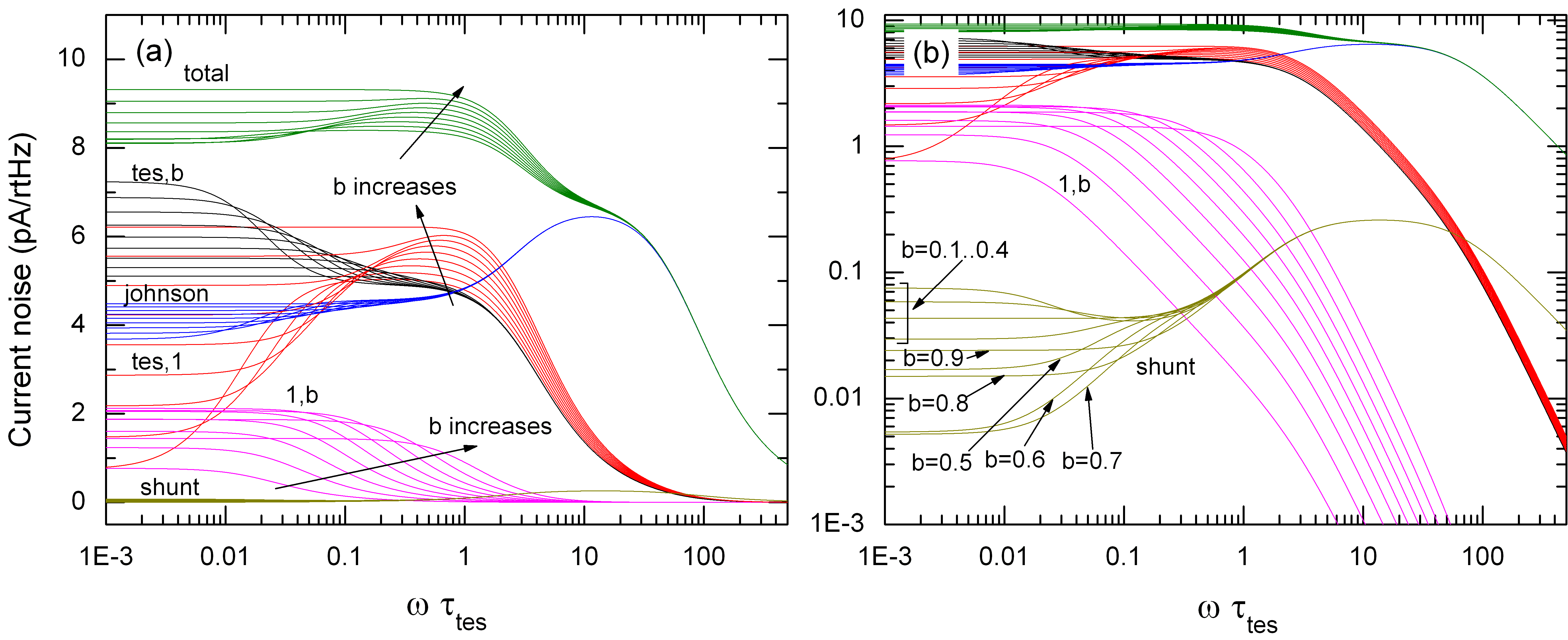
Figure 8: (Color online) Current noise of the two-block parallel model, with varying b=g1,b/[g1,b+gtes,1(T1)]=0.1,0.2,0.3,0.4,0.5,0.6,0.7,0.8,0.9formulae-sequence𝑏subscript𝑔1𝑏delimited-[]subscript𝑔1𝑏subscript𝑔𝑡𝑒𝑠1subscript𝑇10.10.20.30.40.50.60.70.80.9b=g_{1,b}/[g_{1,b}+g_{tes,1}(T_{1})]=0.1,0.2,0.3,0.4,0.5,0.6,0.7,0.8,0.9 in (a) linear-log and (b) log-log scales. Increasing b𝑏b corresponds to a decrease of the low-frequency |Iω|tes,bsubscriptsubscript𝐼𝜔𝑡𝑒𝑠𝑏|I_{\omega}|_{tes,b} noise, increase of the low-frequency |Iω|tes,1subscriptsubscript𝐼𝜔𝑡𝑒𝑠1|I_{\omega}|_{tes,1} noise and a non-monotonous behavior of the |Iω|1,bsubscriptsubscript𝐼𝜔1𝑏|I_{\omega}|_{1,b} noise, with a maximum around b=0.5𝑏0.5b=0.5. Low-frequency Johnson noise increases, and shunt noise has a minimum around b=0.7𝑏0.7b=0.7. Other parameters: =1.651.65{\cal L}=1.65, C1/Ctes=10subscript𝐶1subscript𝐶𝑡𝑒𝑠10C_{1}/C_{tes}=10, a=gtes,1/(gtes,1+gtes,b)=0.5𝑎subscript𝑔𝑡𝑒𝑠1subscript𝑔𝑡𝑒𝑠1subscript𝑔𝑡𝑒𝑠𝑏0.5a=g_{tes,1}/(g_{tes,1}+g_{tes,b})=0.5, R0=0.1Ωsubscript𝑅00.1ΩR_{0}=0.1\mathrm{\Omega}, β=1𝛽1\beta=1, RL=0.001Ωsubscript𝑅𝐿0.001ΩR_{L}=0.001\mathrm{\Omega}, I0=10μsubscript𝐼010𝜇I_{0}=10\muA, g1,b=1subscript𝑔1𝑏1g_{1,b}=1 nW/K, τel=L/[RL+R0(1+β)]=0.015τtessubscript𝜏𝑒𝑙𝐿delimited-[]subscript𝑅𝐿subscript𝑅01𝛽0.015subscript𝜏𝑡𝑒𝑠\tau_{el}=L/[R_{L}+R_{0}(1+\beta)]=0.015\tau_{tes}, τtes=Ctes/gtes,bsubscript𝜏𝑡𝑒𝑠subscript𝐶𝑡𝑒𝑠subscript𝑔𝑡𝑒𝑠𝑏\tau_{tes}=C_{tes}/g_{tes,b}.

In Fig. 8, we show how the different noise components evolve as a function of the thermal conductance g1,bsubscript𝑔1𝑏g_{1,b}. This means that the starting point is the hanging model with g1,b=0subscript𝑔1𝑏0g_{1,b}=0. Again, T1subscript𝑇1T_{1} was calculated using the simplifying assumption n=m=4𝑛𝑚4n=m=4. The general picture is that the total noise increases as g1,bsubscript𝑔1𝑏g_{1,b} increases, parametrized in the plot as b=g1,b/[g1,b+gtes,1(T1)]𝑏subscript𝑔1𝑏delimited-[]subscript𝑔1𝑏subscript𝑔𝑡𝑒𝑠1subscript𝑇1b=g_{1,b}/[g_{1,b}+g_{tes,1}(T_{1})]. In terms of the noise components, the low-frequency shoulder of the phonon noise |Iω|tes,bsubscriptsubscript𝐼𝜔𝑡𝑒𝑠𝑏|I_{\omega}|_{tes,b} decreases, and when b>0.8𝑏0.8b>0.8, the phonon noise becomes flat up to the thermal cut-off frequency. On the other hand, the hanging TFN noise |Iω|tes,1subscriptsubscript𝐼𝜔𝑡𝑒𝑠1|I_{\omega}|_{tes,1} develops an increasing low-frequency level (as in the intermediate model) quite fast, eventually surpassing the low frequency noise contribution from the phonon noise at around b=0.70.8𝑏0.70.8b=0.7-0.8. In addition, the intermediate frequency bump size also increases with b𝑏b, and moves to higher frequencies. The TFN noise component produced by the direct coupling of C1subscript𝐶1C_{1} to bath, |Iω|1,bsubscriptsubscript𝐼𝜔1𝑏|I_{\omega}|_{1,b}, has only a low frequency component, whose cut-off moves up in frequency monotonously with b𝑏b. Also, the strength of the cut-off for |Iω|1,bsubscriptsubscript𝐼𝜔1𝑏|I_{\omega}|_{1,b} increases with b𝑏b, as can be seen from the log-log plot, Fig. 8 (b). This is in contrast to the other two TFN noise components. The noise level for |Iω|1,bsubscriptsubscript𝐼𝜔1𝑏|I_{\omega}|_{1,b} initially increases, but then reaches a maximum around b=0.5𝑏0.5b=0.5, after which it starts decreasing. For the parameter values chosen here, this last TFN component |Iω|1,bsubscriptsubscript𝐼𝜔1𝑏|I_{\omega}|_{1,b} is the smallest, but not insignificant. The low-frequency Johnson noise level increases with b𝑏b, and the shunt noise behaves in a complex manner at low frequencies, where it has the highest value at low b𝑏b, decreases until b=0.7𝑏0.7b=0.7, and then starts increasing again for b>0.7𝑏0.7b>0.7 [See Fig. 8 (b)]. Finally, in the intermediate bump region the total noise increases monotonously with b𝑏b. However, for low frequencies the total noise initially decreases slightly and has a minimum at b=0.20.3𝑏0.20.3b=0.2-0.3 (for the parameter values used), after which the low-frequency part also increases.

III Three-block models

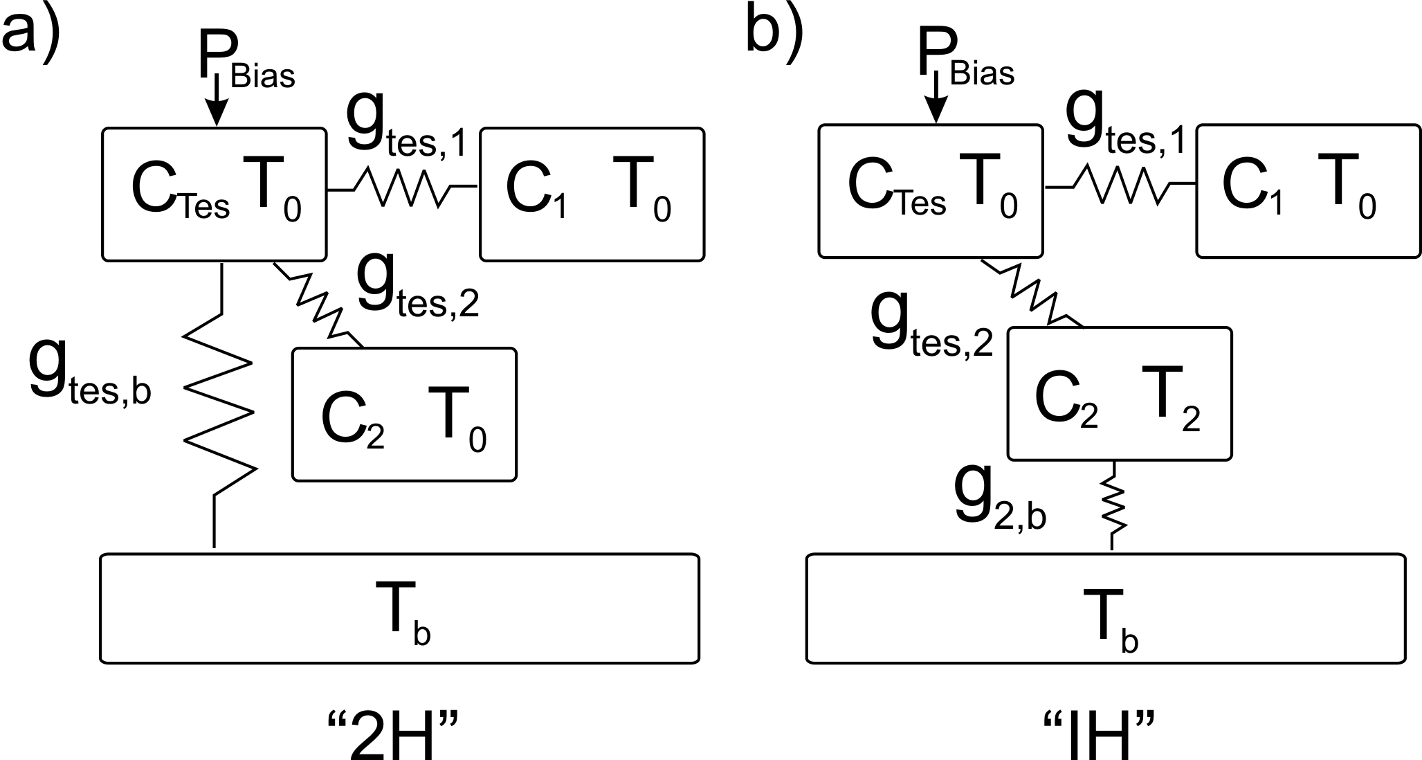
After the exhaustive discussion of the two-block models, we limit ourselves here to two examples of three-block models, which we have already used in analysis of real TES data mikko ; kimmo , see Fig. 9. The first model is the analog of the hanging two-block model, where there are now two hanging extra heat capacities C1subscript𝐶1C_{1} and C2subscript𝐶2C_{2}. We have named this the 2H model. The second model has one intermediate and one hanging block, and we name it the IH model.
Refer to caption
Figure 9: Three-block models studied. (a) 2H model, (b) IH model.

III.1 Equations to be solved

The extension of the differential equations defining the problem for two-block models, Eq. 1, to the equations for three-block models is straightforward. One more equation is generated because of the new heat capacity, and one more power flow term is added, which in the case of the 2H model is C(TtespT2p)𝐶superscriptsubscript𝑇𝑡𝑒𝑠𝑝superscriptsubscript𝑇2𝑝C(T_{tes}^{p}-T_{2}^{p}) in the equation describing Ctessubscript𝐶𝑡𝑒𝑠C_{tes}. Then, after linearization and transformation to frequency domain, the set of equations become for the 2H model

iωTω,tes𝑖𝜔subscript𝑇𝜔𝑡𝑒𝑠\displaystyle i\omega T_{\omega,tes} =\displaystyle= I0R0(2+β)CtesIω1τITω,tes+1τtes,1Tω,1+1τtes,2Tω,2+1CtesPω,subscript𝐼0subscript𝑅02𝛽subscript𝐶𝑡𝑒𝑠subscript𝐼𝜔1subscript𝜏𝐼subscript𝑇𝜔𝑡𝑒𝑠1subscript𝜏𝑡𝑒𝑠1subscript𝑇𝜔11subscript𝜏𝑡𝑒𝑠2subscript𝑇𝜔21subscript𝐶𝑡𝑒𝑠subscript𝑃𝜔\displaystyle\frac{I_{0}R_{0}(2+\beta)}{C_{tes}}I_{\omega}-\frac{1}{\tau_{I}}T_{\omega,tes}+\frac{1}{\tau_{tes,1}}T_{\omega,1}+\frac{1}{\tau_{tes,2}}T_{\omega,2}+\frac{1}{C_{tes}}P_{\omega},
iωTω,1𝑖𝜔subscript𝑇𝜔1\displaystyle i\omega T_{\omega,1} =\displaystyle= 1τ1(Tω,tesTω,1),1subscript𝜏1subscript𝑇𝜔𝑡𝑒𝑠subscript𝑇𝜔1\displaystyle\frac{1}{\tau_{1}}\left(T_{\omega,tes}-T_{\omega,1}\right),
iωTω,2𝑖𝜔subscript𝑇𝜔2\displaystyle i\omega T_{\omega,2} =\displaystyle= 1τ2(Tω,tesTω,2),1subscript𝜏2subscript𝑇𝜔𝑡𝑒𝑠subscript𝑇𝜔2\displaystyle\frac{1}{\tau_{2}}\left(T_{\omega,tes}-T_{\omega,2}\right),
iωLIω𝑖𝜔𝐿subscript𝐼𝜔\displaystyle i\omega LI_{\omega} =\displaystyle= Vω[RL+R0(1+β)]Iω2H(gtes,1+gtes,2+gtes,b)I0Tω,tes,subscript𝑉𝜔delimited-[]subscript𝑅𝐿subscript𝑅01𝛽subscript𝐼𝜔subscript2𝐻subscript𝑔𝑡𝑒𝑠1subscript𝑔𝑡𝑒𝑠2subscript𝑔𝑡𝑒𝑠𝑏subscript𝐼0subscript𝑇𝜔𝑡𝑒𝑠\displaystyle V_{\omega}-\left[R_{L}+R_{0}(1+\beta)\right]I_{\omega}-\frac{{\cal L}_{2H}(g_{tes,1}+g_{tes,2}+g_{tes,b})}{I_{0}}T_{\omega,tes}, (25)

where all gisubscript𝑔𝑖g_{i} are evaluated at T0subscript𝑇0T_{0}, τtes,1=Ctes/gtes,1subscript𝜏𝑡𝑒𝑠1subscript𝐶𝑡𝑒𝑠subscript𝑔𝑡𝑒𝑠1\tau_{tes,1}=C_{tes}/g_{tes,1}, τtes,2=Ctes/gtes,2subscript𝜏𝑡𝑒𝑠2subscript𝐶𝑡𝑒𝑠subscript𝑔𝑡𝑒𝑠2\tau_{tes,2}=C_{tes}/g_{tes,2}, and the definitions of the more important time constants τisubscript𝜏𝑖\tau_{i} and the effective loop gain 2Hsubscript2𝐻{\cal L}_{2H} are now:

τIsubscript𝜏𝐼\displaystyle\tau_{I} =\displaystyle= Ctes(gtes,1+gtes,2+gtes,b)(12H),subscript𝐶𝑡𝑒𝑠subscript𝑔𝑡𝑒𝑠1subscript𝑔𝑡𝑒𝑠2subscript𝑔𝑡𝑒𝑠𝑏1subscript2𝐻\displaystyle\frac{C_{tes}}{(g_{tes,1}+g_{tes,2}+g_{tes,b})(1-{\cal L}_{2H})},
τ1subscript𝜏1\displaystyle\tau_{1} =\displaystyle= C1gtes,1,subscript𝐶1subscript𝑔𝑡𝑒𝑠1\displaystyle\frac{C_{1}}{g_{tes,1}},
τ2subscript𝜏2\displaystyle\tau_{2} =\displaystyle= C2gtes,2,subscript𝐶2subscript𝑔𝑡𝑒𝑠2\displaystyle\frac{C_{2}}{g_{tes,2}},
2Hsubscript2𝐻\displaystyle{\cal L}_{2H} =\displaystyle= P0α(gtes,1+gtes,2+gtes,b)T0.subscript𝑃0𝛼subscript𝑔𝑡𝑒𝑠1subscript𝑔𝑡𝑒𝑠2subscript𝑔𝑡𝑒𝑠𝑏subscript𝑇0\displaystyle\frac{P_{0}\alpha}{(g_{tes,1}+g_{tes,2}+g_{tes,b})T_{0}}. (26)

Comparing to the two-block equations 4, we see that the first equation has one more term due to the added heat capacity C2subscript𝐶2C_{2}, the third equation is new, and the last term in the equation for Iωsubscript𝐼𝜔I_{\omega} has a changed coefficient due to the new thermal conductance gtes,2subscript𝑔𝑡𝑒𝑠2g_{tes,2}.

III.2 Complex impedance

III.2.1 2H model

The complex impedance for the 2H model is calculated from Eqs. 25 the same way as for the two-block models, with the result

Ztes,2H=R0(1+β)+2H12HR0(2+β)/[1+iωτId112H11+iωτ1d212H11+iωτ2],subscript𝑍𝑡𝑒𝑠2𝐻subscript𝑅01𝛽/subscript2𝐻1subscript2𝐻subscript𝑅02𝛽delimited-[]1𝑖𝜔subscript𝜏𝐼subscript𝑑11subscript2𝐻11𝑖𝜔subscript𝜏1subscript𝑑21subscript2𝐻11𝑖𝜔subscript𝜏2Z_{tes,2H}=R_{0}(1+\beta)+\frac{{\cal L}_{2H}}{1-{\cal L}_{2H}}R_{0}(2+\beta)\left/\left[1+i\omega\tau_{I}-\frac{d_{1}}{1-{\cal L}_{2H}}\frac{1}{1+i\omega\tau_{1}}-\frac{d_{2}}{1-{\cal L}_{2H}}\frac{1}{1+i\omega\tau_{2}}\right]\right., (27)

where we have denoted the relative strengths of the thermal conductances as d1=gtes,1/(gtes,1+gtes,2+gtes,b)subscript𝑑1subscript𝑔𝑡𝑒𝑠1subscript𝑔𝑡𝑒𝑠1subscript𝑔𝑡𝑒𝑠2subscript𝑔𝑡𝑒𝑠𝑏d_{1}=g_{tes,1}/(g_{tes,1}+g_{tes,2}+g_{tes,b}) and d2=gtes,2/(gtes,1+gtes,2+gtes,b)subscript𝑑2subscript𝑔𝑡𝑒𝑠2subscript𝑔𝑡𝑒𝑠1subscript𝑔𝑡𝑒𝑠2subscript𝑔𝑡𝑒𝑠𝑏d_{2}=g_{tes,2}/(g_{tes,1}+g_{tes,2}+g_{tes,b}), and other symbols are defined in Eqs. 26. By comparing with the result for the hanging two-block model, Eq. 6, we see that because of the added C2subscript𝐶2C_{2}, a new term appears in the denominator. This term is naturally mathematically equivalent with the term for C1subscript𝐶1C_{1}, as both C1subscript𝐶1C_{1} and C2subscript𝐶2C_{2} are hanging in this model. However, one should bear in mind that the term for C1subscript𝐶1C_{1} is not exactly the same as in the hanging two-block model, because the new thermal conductance gtes,2subscript𝑔𝑡𝑒𝑠2g_{tes,2} also affects it through the pre-factor d1subscript𝑑1d_{1}. Also, one sees from Eq. 27 that the effect of C2subscript𝐶2C_{2} is not additive, as the new term is in the denominator. It is therefore not obvious how Ztes,2Hsubscript𝑍𝑡𝑒𝑠2𝐻Z_{tes,2H} behaves as a function of the new thermal parameters C2subscript𝐶2C_{2} and gtes,2subscript𝑔𝑡𝑒𝑠2g_{tes,2}, and we therefore investigate their effect by examples, shown in Fig. 10.
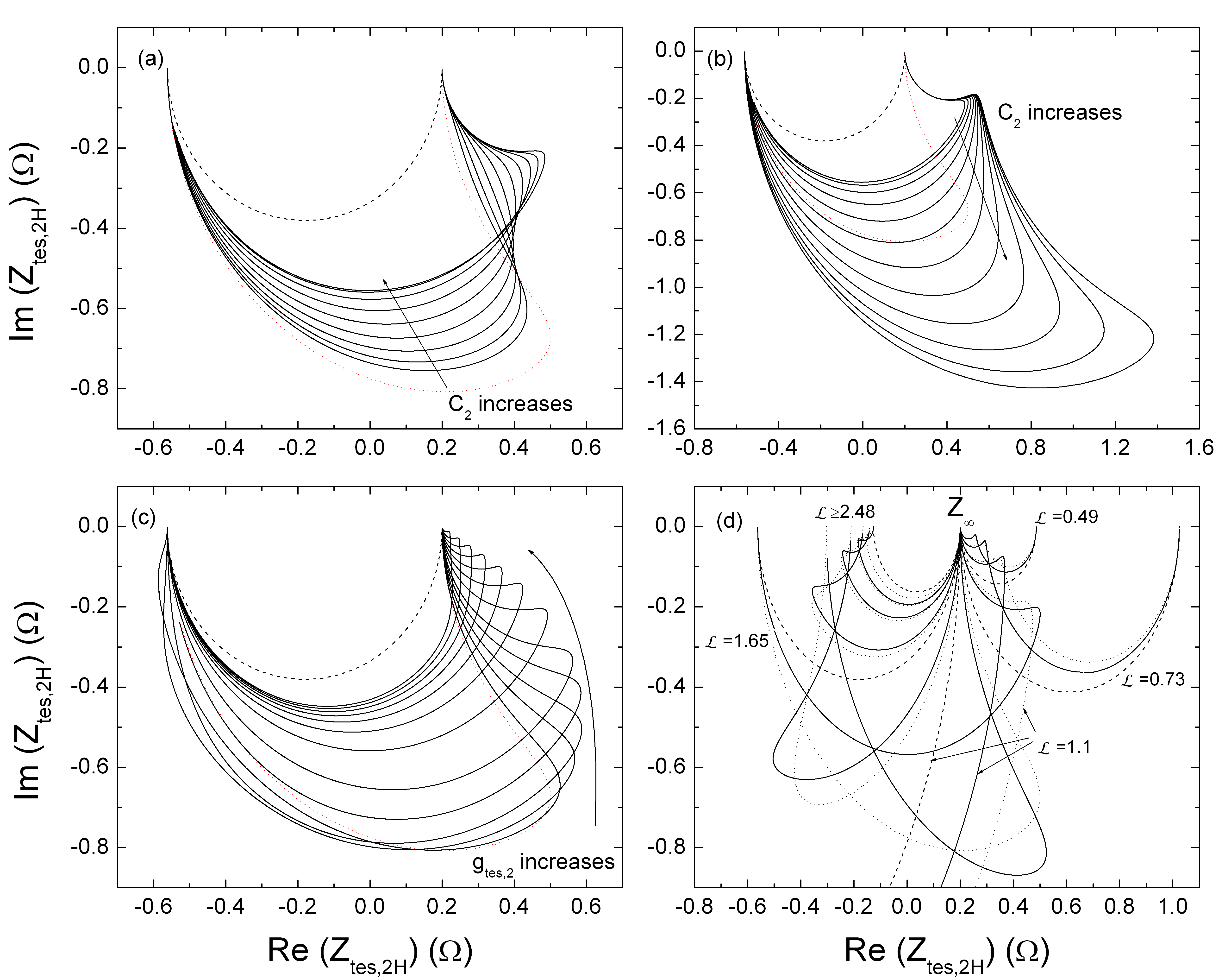
Refer to caption
Figure 10: Complex impedance of the three-block 2H model, with varying parameters. We have used R0=0.1Ωsubscript𝑅00.1ΩR_{0}=0.1\mathrm{\Omega} and β=1𝛽1\beta=1 in all plots, and frequencies run typically between ωτtes=0.01..100𝜔subscript𝜏𝑡𝑒𝑠0.01..100\omega\tau_{tes}=0.01..100 (for some curves 104..100superscript104..10010^{-4}..100), with τtes=Ctes/gtes,bsubscript𝜏𝑡𝑒𝑠subscript𝐶𝑡𝑒𝑠subscript𝑔𝑡𝑒𝑠𝑏\tau_{tes}=C_{tes}/g_{tes,b}. (a) Ztes,2Hsubscript𝑍𝑡𝑒𝑠2𝐻Z_{tes,2H} as a function of C2subscript𝐶2C_{2}, with C2/Ctes=0.33,0.49,0.73,1.1,1.65,2.48,3.71,5.57,8.35subscript𝐶2subscript𝐶𝑡𝑒𝑠0.330.490.731.11.652.483.715.578.35C_{2}/C_{tes}=0.33,0.49,0.73,1.1,1.65,2.48,3.71,5.57,8.35, C1/Ctes=10subscript𝐶1subscript𝐶𝑡𝑒𝑠10C_{1}/C_{tes}=10, =1.651.65{\cal L}=1.65, a=gtes,1/(gtes,1+gtes,b)=0.5𝑎subscript𝑔𝑡𝑒𝑠1subscript𝑔𝑡𝑒𝑠1subscript𝑔𝑡𝑒𝑠𝑏0.5a=g_{tes,1}/(g_{tes,1}+g_{tes,b})=0.5 and d2=gtes,2/(gtes,1+gtes,2+gtes,b)=0.3subscript𝑑2subscript𝑔𝑡𝑒𝑠2subscript𝑔𝑡𝑒𝑠1subscript𝑔𝑡𝑒𝑠2subscript𝑔𝑡𝑒𝑠𝑏0.3d_{2}=g_{tes,2}/(g_{tes,1}+g_{tes,2}+g_{tes,b})=0.3. Increasing C2subscript𝐶2C_{2} corresponds to a shrinking of the bulge caused by C1subscript𝐶1C_{1}, and a growth of a second one at higher frequencies. The two-block model limit (C2=0subscript𝐶20C_{2}=0) is shown as the red dotted line, and the one-block limit (C1=0subscript𝐶10C_{1}=0) as the dashed line. (b) Same, but with C2/Ctes=8.35,12.5,18.8,28.2,42.3,63.4,95.1,142.7,214.1,321.1,481.7,722.5subscript𝐶2subscript𝐶𝑡𝑒𝑠8.3512.518.828.242.363.495.1142.7214.1321.1481.7722.5C_{2}/C_{tes}=8.35,12.5,18.8,28.2,42.3,63.4,95.1,142.7,214.1,321.1,481.7,722.5. Increasing C2subscript𝐶2C_{2} corresponds to a growth of the bulge. The dotted and dashed lines are the same as in (a). (c) Ztes,2Hsubscript𝑍𝑡𝑒𝑠2𝐻Z_{tes,2H} as a function of d2subscript𝑑2d_{2} (or gtes,2subscript𝑔𝑡𝑒𝑠2g_{tes,2}), with d2=0.02,0.06,0.1,0.15,0.2,0.3,0.4,0.5,0.6,0.7,0.8,0.9subscript𝑑20.020.060.10.150.20.30.40.50.60.70.80.9d_{2}=0.02,0.06,0.1,0.15,0.2,0.3,0.4,0.5,0.6,0.7,0.8,0.9, =1.651.65{\cal L}=1.65, C1/Ctes=10subscript𝐶1subscript𝐶𝑡𝑒𝑠10C_{1}/C_{tes}=10, C2/Ctes=10subscript𝐶2subscript𝐶𝑡𝑒𝑠10C_{2}/C_{tes}=10, and a=0.5𝑎0.5a=0.5. Increasing d2subscript𝑑2d_{2} corresponds to the added bulge feature moving from the left, low-frequency side to the right, high-frequency side. The dotted and dashed lines are the same as in (a). (d) Ztes,2Hsubscript𝑍𝑡𝑒𝑠2𝐻Z_{tes,2H} as a function of =P0α/(gtes,bT0)subscript𝑃0𝛼subscript𝑔𝑡𝑒𝑠𝑏subscript𝑇0{\cal L}=P_{0}\alpha/(g_{tes,b}T_{0}), with =0.49,0.73,1.1,1.65,2.48,3.71,5.57,8.35,12.50.490.731.11.652.483.715.578.3512.5{\cal L}=0.49,0.73,1.1,1.65,2.48,3.71,5.57,8.35,12.5, C1/Ctes=10subscript𝐶1subscript𝐶𝑡𝑒𝑠10C_{1}/C_{tes}=10, C2/Ctes=10subscript𝐶2subscript𝐶𝑡𝑒𝑠10C_{2}/C_{tes}=10, d2=0.3subscript𝑑20.3d_{2}=0.3 and a=0.5𝑎0.5a=0.5. The two-block limits (C2=0subscript𝐶20C_{2}=0) are shown as dotted lines, and some one-block results as dashed lines.

What we observe from Figs. 10 (a) and (b) is that by increasing C2subscript𝐶2C_{2}, the bulge feature caused by C1subscript𝐶1C_{1} first gets smaller, and starts to be pushed to a higher frequency (further right). However, when C2C1subscript𝐶2subscript𝐶1C_{2}\approx C_{1}, the trend turns and the bulge feature at the original place also starts increasing again. Importantly, for C2C1subscript𝐶2subscript𝐶1C_{2}\leq C_{1} the new term does not necessarily lead to a new, additive bulge in the complex plane, but just contributes to the old, existing one by changing its shape. As a function of d2=gtes,2/(gtes,1+gtes,2+gtes,b)subscript𝑑2subscript𝑔𝑡𝑒𝑠2subscript𝑔𝑡𝑒𝑠1subscript𝑔𝑡𝑒𝑠2subscript𝑔𝑡𝑒𝑠𝑏d_{2}=g_{tes,2}/(g_{tes,1}+g_{tes,2}+g_{tes,b}) [Fig. 10 (c)] , things look a bit like for parameter a𝑎a in the two-block case. Interestingly, there is always an increased bulge compared to the two-block model on the high frequency side, but also on low frequency side for small d2<0.15subscript𝑑20.15d_{2}<0.15 for these parameter values. In the limit d21subscript𝑑21d_{2}\rightarrow 1 Ztes,2Hsubscript𝑍𝑡𝑒𝑠2𝐻Z_{tes,2H} approaches a two-block model with a higher effective TES heat capacity Ctes+C2subscript𝐶𝑡𝑒𝑠subscript𝐶2C_{tes}+C_{2}. The loop gain again has a complex effect, as shown in Fig. 2 (d). In the large loop gain limit, the three-block hanging model approaches the simple model, but more slowly than in the two-block case. For typical values of {\cal L} the effect of the added term is strong, as can be seen by comparing the two- and three block results.

III.2.2 IH model

The starting equations for the IH model look just slightly different from the 2H case, as the thermal conductances couple different heat capacities, which can be at different steady state temperatures (T0subscript𝑇0T_{0} for Ctessubscript𝐶𝑡𝑒𝑠C_{tes} and C1subscript𝐶1C_{1}, and T2subscript𝑇2T_{2} for C2subscript𝐶2C_{2}). The derivation thus follows analogously to the 2H model, and we simply quote the end result for the complex impedance. It looks mathematically exactly the same as the result for the 2H model, with only some changes in parametrization:

Ztes,IH=R0(1+β)+IH1IHR0(2+β)/[1+iωτId11IH11+iωτ1d21IH11+iωτ2],subscript𝑍𝑡𝑒𝑠𝐼𝐻subscript𝑅01𝛽/subscript𝐼𝐻1subscript𝐼𝐻subscript𝑅02𝛽delimited-[]1𝑖𝜔subscript𝜏𝐼subscript𝑑11subscript𝐼𝐻11𝑖𝜔subscript𝜏1subscript𝑑21subscript𝐼𝐻11𝑖𝜔subscript𝜏2Z_{tes,IH}=R_{0}(1+\beta)+\frac{{\cal L}_{IH}}{1-{\cal L}_{IH}}R_{0}(2+\beta)\left/\left[1+i\omega\tau_{I}-\frac{d_{1}}{1-{\cal L}_{IH}}\frac{1}{1+i\omega\tau_{1}}-\frac{d_{2}}{1-{\cal L}_{IH}}\frac{1}{1+i\omega\tau_{2}}\right]\right., (28)

where the definitions of the prefactors disubscript𝑑𝑖d_{i}, the time constants τisubscript𝜏𝑖\tau_{i} and the effective loop gain IHsubscript𝐼𝐻{\cal L}_{IH} are now:

d1subscript𝑑1\displaystyle d_{1} =\displaystyle= gtes,1gtes,1+gtes,2(T0)subscript𝑔𝑡𝑒𝑠1subscript𝑔𝑡𝑒𝑠1subscript𝑔𝑡𝑒𝑠2subscript𝑇0\displaystyle\frac{g_{tes,1}}{g_{tes,1}+g_{tes,2}(T_{0})}
d2subscript𝑑2\displaystyle d_{2} =\displaystyle= gtes,2(T0)gtes,2(T2)(gtes,1+gtes,2(T0))(gtes,2(T2)+g2,b)subscript𝑔𝑡𝑒𝑠2subscript𝑇0subscript𝑔𝑡𝑒𝑠2subscript𝑇2subscript𝑔𝑡𝑒𝑠1subscript𝑔𝑡𝑒𝑠2subscript𝑇0subscript𝑔𝑡𝑒𝑠2subscript𝑇2subscript𝑔2𝑏\displaystyle\frac{g_{tes,2}(T_{0})g_{tes,2}(T_{2})}{(g_{tes,1}+g_{tes,2}(T_{0}))(g_{tes,2}(T_{2})+g_{2,b})}
τIsubscript𝜏𝐼\displaystyle\tau_{I} =\displaystyle= Ctes[gtes,1+gtes,2(T0)](1IH),subscript𝐶𝑡𝑒𝑠delimited-[]subscript𝑔𝑡𝑒𝑠1subscript𝑔𝑡𝑒𝑠2subscript𝑇01subscript𝐼𝐻\displaystyle\frac{C_{tes}}{[g_{tes,1}+g_{tes,2}(T_{0})](1-{\cal L}_{IH})},
τ1subscript𝜏1\displaystyle\tau_{1} =\displaystyle= C1gtes,1,subscript𝐶1subscript𝑔𝑡𝑒𝑠1\displaystyle\frac{C_{1}}{g_{tes,1}},
τ2subscript𝜏2\displaystyle\tau_{2} =\displaystyle= C2gtes,2(T2)+g2,b,subscript𝐶2subscript𝑔𝑡𝑒𝑠2subscript𝑇2subscript𝑔2𝑏\displaystyle\frac{C_{2}}{g_{tes,2}(T_{2})+g_{2,b}},
IHsubscript𝐼𝐻\displaystyle{\cal L}_{IH} =\displaystyle= P0α[gtes,1+gtes,2(T0)]T0.subscript𝑃0𝛼delimited-[]subscript𝑔𝑡𝑒𝑠1subscript𝑔𝑡𝑒𝑠2subscript𝑇0subscript𝑇0\displaystyle\frac{P_{0}\alpha}{[g_{tes,1}+g_{tes,2}(T_{0})]T_{0}}. (29)

gtes,1subscript𝑔𝑡𝑒𝑠1g_{tes,1} is always evaluated at T0subscript𝑇0T_{0} and g2,bsubscript𝑔2𝑏g_{2,b} at T2subscript𝑇2T_{2}, therefore we have omitted the temperature dependence from their notation for simplification. g2,b(Tb)subscript𝑔2𝑏subscript𝑇𝑏g_{2,b}(T_{b}) will only come into play through Eq. 18, when calculating the noise amplitude. The true loop gain is again the same as for the intermediate two-block model (if one takes into account the notation change C1C2subscript𝐶1subscript𝐶2C_{1}\rightarrow C_{2}), given by =P0α/(geffT0)subscript𝑃0𝛼subscript𝑔𝑒𝑓𝑓subscript𝑇0{\cal L}=P_{0}\alpha/(g_{eff}T_{0}), where

geff=gtes,2(T0)g2,bgtes,2(T2)+g2,b.subscript𝑔𝑒𝑓𝑓subscript𝑔𝑡𝑒𝑠2subscript𝑇0subscript𝑔2𝑏subscript𝑔𝑡𝑒𝑠2subscript𝑇2subscript𝑔2𝑏g_{eff}=\frac{g_{tes,2}(T_{0})g_{2,b}}{g_{tes,2}(T_{2})+g_{2,b}}. (30)

Because of the mathematical equivalence between Ztes,2Hsubscript𝑍𝑡𝑒𝑠2𝐻Z_{tes,2H} and Ztes,IHsubscript𝑍𝑡𝑒𝑠𝐼𝐻Z_{tes,IH}, we do not discuss the details further here, similar plots to Fig. 10 could be generated.

III.3 Small-signal responsivity

Again, derivation of the linear responsivity is straightforward using Eqs. 25 or the equivalent ones for the IH model. As the model dependent terms can all be lumped into Ztessubscript𝑍𝑡𝑒𝑠Z_{tes}, both three-block models also satisfy Equation 15. In Fig. 11 we plot examples of how |sI(ω)|subscript𝑠𝐼𝜔|s_{I}(\omega)| behaves for the 2H model, similar plots would also follow for the IH model. The overall behavior is the same as with the two-block models, with a partial thermal cut-off moving to lower frequencies with increasing C2subscript𝐶2C_{2}, and a decrease of responsivity above that partial thermal cut-off with increasing d2=gtes,2/(gtes,1+gtes,2+gtes,b)subscript𝑑2subscript𝑔𝑡𝑒𝑠2subscript𝑔𝑡𝑒𝑠1subscript𝑔𝑡𝑒𝑠2subscript𝑔𝑡𝑒𝑠𝑏d_{2}=g_{tes,2}/(g_{tes,1}+g_{tes,2}+g_{tes,b}). A notable difference to the two-block results is that for some values of the parameters C2subscript𝐶2C_{2} and d2subscript𝑑2d_{2} [C2>C1subscript𝐶2subscript𝐶1C_{2}>C_{1} in Fig. 11 (a) and d2<0.6subscript𝑑20.6d_{2}<0.6 in Fig. 11 (b)], the responsivity shows a ”double knee” structure.
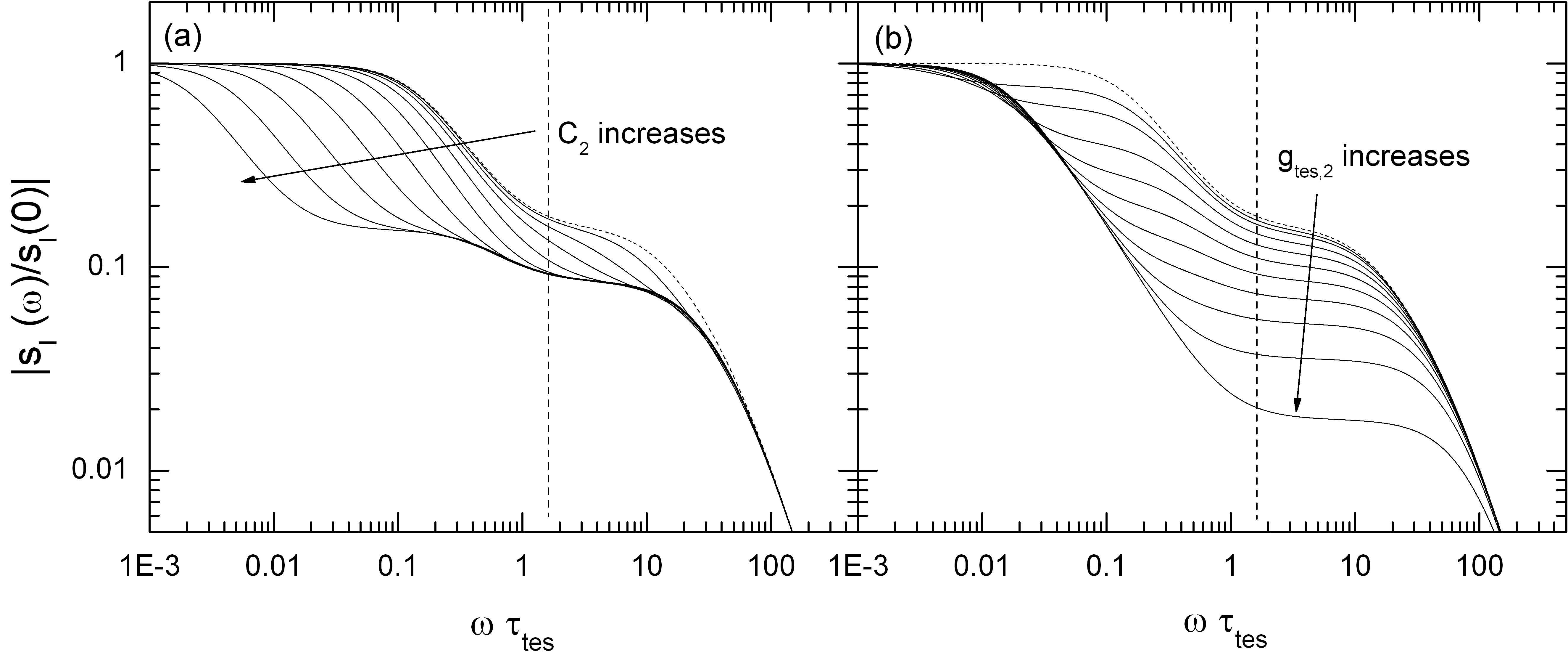
Refer to caption
Figure 11: Responsivity of a three-block 2H model, with varying thermal parameters. (a) |sI(ω)|subscript𝑠𝐼𝜔|s_{I}(\omega)| as a function of C2subscript𝐶2C_{2}, with C2/Ctes=0.33,1.1,2.48,5.57,12.5,28.2,63.4,142.7,321.1,722.5subscript𝐶2subscript𝐶𝑡𝑒𝑠0.331.12.485.5712.528.263.4142.7321.1722.5C_{2}/C_{tes}=0.33,1.1,2.48,5.57,12.5,28.2,63.4,142.7,321.1,722.5, and d2=gtes,2/(gtes,1+gtes,2+gtes,b)=0.5subscript𝑑2subscript𝑔𝑡𝑒𝑠2subscript𝑔𝑡𝑒𝑠1subscript𝑔𝑡𝑒𝑠2subscript𝑔𝑡𝑒𝑠𝑏0.5d_{2}=g_{tes,2}/(g_{tes,1}+g_{tes,2}+g_{tes,b})=0.5. Increasing C2subscript𝐶2C_{2} corresponds to a shift of the first partial thermal cut-off to lower frequencies and the development of a ”double knee” in the intermediate frequency range. (b) |sI(ω)|subscript𝑠𝐼𝜔|s_{I}(\omega)| as a function of d2subscript𝑑2d_{2} (or gtes,2subscript𝑔𝑡𝑒𝑠2g_{tes,2}), with d2=0.05,0.1,0.2,0.3,0.4,0.5,0.6,0.7,0.8,0.9subscript𝑑20.050.10.20.30.40.50.60.70.80.9d_{2}=0.05,0.1,0.2,0.3,0.4,0.5,0.6,0.7,0.8,0.9, C2/Ctes=100subscript𝐶2subscript𝐶𝑡𝑒𝑠100C_{2}/C_{tes}=100. Increasing d2subscript𝑑2d_{2} corresponds to the decrease of responsivity. We have used R0=0.1Ωsubscript𝑅00.1ΩR_{0}=0.1\mathrm{\Omega}, β=1𝛽1\beta=1, τel=L/[RL+R0(1+β)]=0.015τtessubscript𝜏𝑒𝑙𝐿delimited-[]subscript𝑅𝐿subscript𝑅01𝛽0.015subscript𝜏𝑡𝑒𝑠\tau_{el}=L/[R_{L}+R_{0}(1+\beta)]=0.015\tau_{tes}, C1/Ctes=10subscript𝐶1subscript𝐶𝑡𝑒𝑠10C_{1}/C_{tes}=10, a=gtes,1/(gtes,1+gtes,b)=0.9𝑎subscript𝑔𝑡𝑒𝑠1subscript𝑔𝑡𝑒𝑠1subscript𝑔𝑡𝑒𝑠𝑏0.9a=g_{tes,1}/(g_{tes,1}+g_{tes,b})=0.9 and =1.651.65{\cal L}=1.65 in all plots (if not varied). τtes=Ctes/gtes,bsubscript𝜏𝑡𝑒𝑠subscript𝐶𝑡𝑒𝑠subscript𝑔𝑡𝑒𝑠𝑏\tau_{tes}=C_{tes}/g_{tes,b}. Dashed vertical line shows the simple model effective thermal time constant, and dotted curves the corresponding two-block results (limit C2=0subscript𝐶20C_{2}=0).

III.4 Thermodynamic noise

III.4.1 2H model

Thermal fluctuation noise

The thermal fluctuation noise components for the 2H model can be derived analogously to the two-block models, by adding the power fluctuation terms to equations 25. Straightforward algebra then yields for the three TFN noise components

|Iω|tes,12subscriptsuperscriptsubscript𝐼𝜔2𝑡𝑒𝑠1\displaystyle|I_{\omega}|^{2}_{tes,1} =\displaystyle= Ptes,12|sI(ω)|2ω2τ121+ω2τ12,superscriptsubscript𝑃𝑡𝑒𝑠12superscriptsubscript𝑠𝐼𝜔2superscript𝜔2superscriptsubscript𝜏121superscript𝜔2superscriptsubscript𝜏12\displaystyle P_{tes,1}^{2}|s_{I}(\omega)|^{2}\frac{\omega^{2}\tau_{1}^{2}}{1+\omega^{2}\tau_{1}^{2}},
|Iω|tes,22subscriptsuperscriptsubscript𝐼𝜔2𝑡𝑒𝑠2\displaystyle|I_{\omega}|^{2}_{tes,2} =\displaystyle= Ptes,22|sI(ω)|2ω2τ221+ω2τ22,superscriptsubscript𝑃𝑡𝑒𝑠22superscriptsubscript𝑠𝐼𝜔2superscript𝜔2superscriptsubscript𝜏221superscript𝜔2superscriptsubscript𝜏22\displaystyle P_{tes,2}^{2}|s_{I}(\omega)|^{2}\frac{\omega^{2}\tau_{2}^{2}}{1+\omega^{2}\tau_{2}^{2}},
|Iω|tes,b2subscriptsuperscriptsubscript𝐼𝜔2𝑡𝑒𝑠𝑏\displaystyle|I_{\omega}|^{2}_{tes,b} =\displaystyle= Ptes,b2|sI(ω)|2,superscriptsubscript𝑃𝑡𝑒𝑠𝑏2superscriptsubscript𝑠𝐼𝜔2\displaystyle P_{tes,b}^{2}|s_{I}(\omega)|^{2}, (31)

if we assume that the three TFN noise sources are all uncorrelated with each other. The power noise amplitudes Pisubscript𝑃𝑖P_{i} are defined as before by Eq. 18, and the time constants as τi=Ci/gtes,isubscript𝜏𝑖subscript𝐶𝑖subscript𝑔𝑡𝑒𝑠𝑖\tau_{i}=C_{i}/g_{tes,i}, just as for the impedance in Eqs. 26.

Johnson noise terms

Again, we can derive the TES Johnson noise using the internal impedance matrix formulation of section II.4.1. Just as in the case of responsivity, the end result is that the thermal model dependency is fully accounted for by the TES complex impedance, so that Eq. 20 is still valid. The same applies to the external (shunt) Johnson noise term, where Eq. 21 can still be used.

We skip plotting the noise for the 2H model, as Eqs. 31 clearly show that the overall picture is analogous to the two-block hanging model. Now, we simply have two independent TFN noise bumps, which are multiplied by the responsivity curves shown in Fig. 11. Because of the monotonously decreasing shape of |sI(ω)|subscript𝑠𝐼𝜔|s_{I}(\omega)|, the higher frequency TFN noise bump is always suppressed more than the lower frequency bump.

III.4.2 IH model

For the IH model, the TFN current noise terms are naturally derived similarily, with the result

|Iω|tes,12subscriptsuperscriptsubscript𝐼𝜔2𝑡𝑒𝑠1\displaystyle|I_{\omega}|^{2}_{tes,1} =\displaystyle= Ptes,12|sI(ω)|2ω2τ121+ω2τ12,superscriptsubscript𝑃𝑡𝑒𝑠12superscriptsubscript𝑠𝐼𝜔2superscript𝜔2superscriptsubscript𝜏121superscript𝜔2superscriptsubscript𝜏12\displaystyle P_{tes,1}^{2}|s_{I}(\omega)|^{2}\frac{\omega^{2}\tau_{1}^{2}}{1+\omega^{2}\tau_{1}^{2}},
|Iω|tes,22subscriptsuperscriptsubscript𝐼𝜔2𝑡𝑒𝑠2\displaystyle|I_{\omega}|^{2}_{tes,2} =\displaystyle= Ptes,12|sI(ω)|2g2,b2/(gtes,2(T2)+g2,b)2+ω2τ221+ω2τ22,superscriptsubscript𝑃𝑡𝑒𝑠12superscriptsubscript𝑠𝐼𝜔2superscriptsubscript𝑔2𝑏2superscriptsubscript𝑔𝑡𝑒𝑠2subscript𝑇2subscript𝑔2𝑏2superscript𝜔2superscriptsubscript𝜏221superscript𝜔2superscriptsubscript𝜏22\displaystyle P_{tes,1}^{2}|s_{I}(\omega)|^{2}\frac{g_{2,b}^{2}/(g_{tes,2}(T_{2})+g_{2,b})^{2}+\omega^{2}\tau_{2}^{2}}{1+\omega^{2}\tau_{2}^{2}},
|Iω|2,b2subscriptsuperscriptsubscript𝐼𝜔22𝑏\displaystyle|I_{\omega}|^{2}_{2,b} =\displaystyle= P2,b2|sI(ω)|2gtes,22(T2)(gtes,2(T2)+g2,b)211+ω2τ22,superscriptsubscript𝑃2𝑏2superscriptsubscript𝑠𝐼𝜔2superscriptsubscript𝑔𝑡𝑒𝑠22subscript𝑇2superscriptsubscript𝑔𝑡𝑒𝑠2subscript𝑇2subscript𝑔2𝑏211superscript𝜔2superscriptsubscript𝜏22\displaystyle P_{2,b}^{2}|s_{I}(\omega)|^{2}\frac{g_{tes,2}^{2}(T_{2})}{(g_{tes,2}(T_{2})+g_{2,b})^{2}}\frac{1}{1+\omega^{2}\tau_{2}^{2}}, (32)

where τ1=C1/gtes,1subscript𝜏1subscript𝐶1subscript𝑔𝑡𝑒𝑠1\tau_{1}=C_{1}/g_{tes,1} and τ2=C2/(gtes,2(T2)+g2,b)subscript𝜏2subscript𝐶2subscript𝑔𝑡𝑒𝑠2subscript𝑇2subscript𝑔2𝑏\tau_{2}=C_{2}/(g_{tes,2}(T_{2})+g_{2,b}), as before for the IH model. The Johnson noise for the TES and the shunt follow again from the general formulas Eq. 20 and Eq. 21.
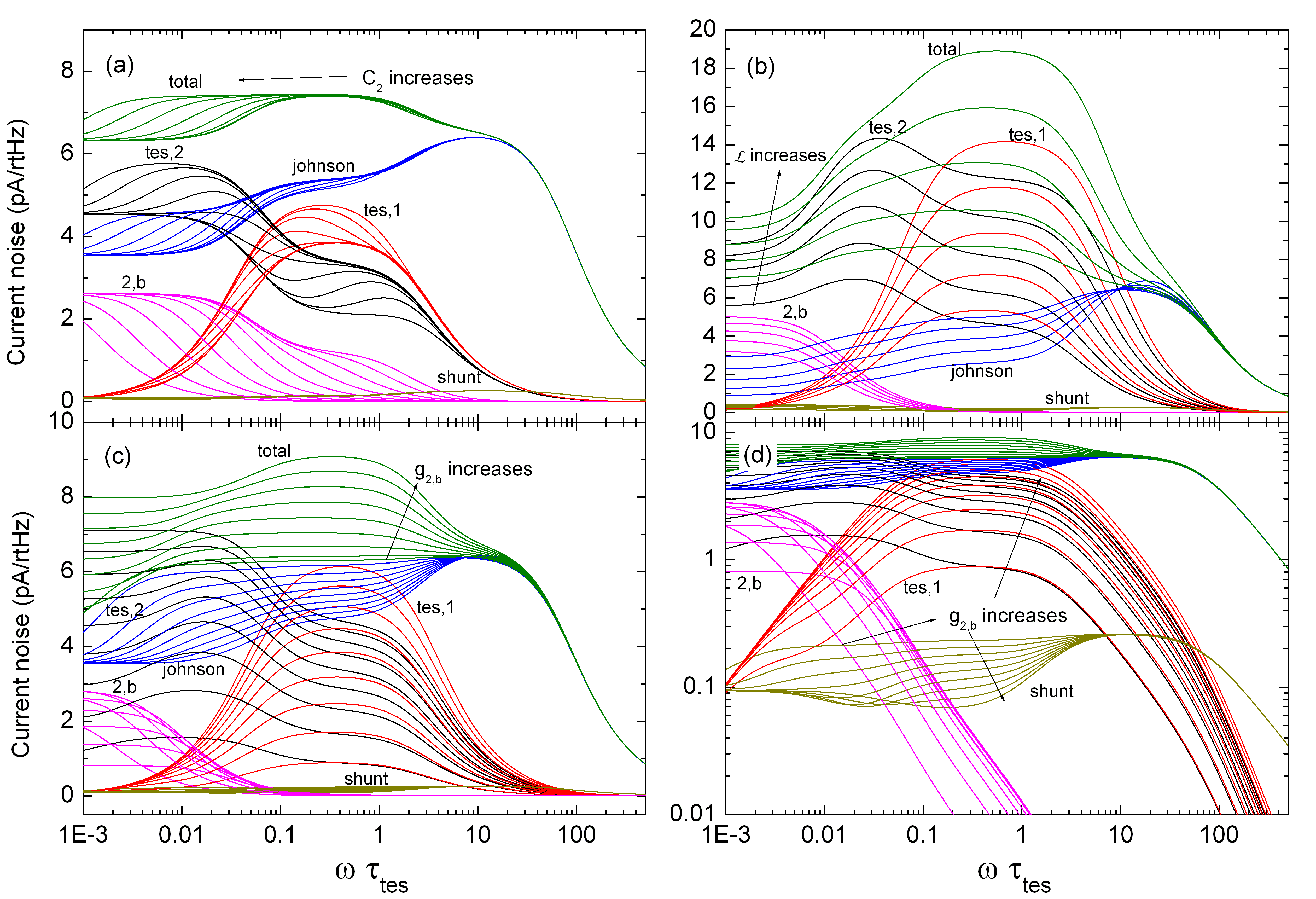
Refer to caption
Figure 12: (Color online) Current noise of a three-block IH model, (a) with varying C2/Ctes=0.49,1.1,2.48,5.57,12.5,28.2,63.4,142.7,321.1,722.5subscript𝐶2subscript𝐶𝑡𝑒𝑠0.491.12.485.5712.528.263.4142.7321.1722.5C_{2}/C_{tes}=0.49,1.1,2.48,5.57,12.5,28.2,63.4,142.7,321.1,722.5 in linear-log scale. Increasing C2subscript𝐶2C_{2} corresponds to a shift of the onset of the total noise bump to lower frequencies, an addition of a bump feature in |Iω|tes,2subscriptsubscript𝐼𝜔𝑡𝑒𝑠2|I_{\omega}|_{tes,2} that moves to lower frequencies, a reduction of the |Iω|tes,1subscriptsubscript𝐼𝜔𝑡𝑒𝑠1|I_{\omega}|_{tes,1} noise component, and a decrease of the cut-off frequency for the |Iω|2,bsubscriptsubscript𝐼𝜔2𝑏|I_{\omega}|_{2,b} noise component. Mid-frequency Johnson noise also increases. (b) Same, with varying =2.48,3.71,5.57,8.35,12.52.483.715.578.3512.5{\cal L}=2.48,3.71,5.57,8.35,12.5. Increasing {\cal L} corresponds to an increase of the TFN noise levels, and a decrease of the low-frequency Johnson noise. (c) Same, with varying c=g2,b/(gtes,2(T2)+g2,b)=0.1,0.2,0.3,0.4,0.5,0.6,0.7,0.8,0.9formulae-sequence𝑐subscript𝑔2𝑏subscript𝑔𝑡𝑒𝑠2subscript𝑇2subscript𝑔2𝑏0.10.20.30.40.50.60.70.80.9c=g_{2,b}/(g_{tes,2}(T_{2})+g_{2,b})=0.1,0.2,0.3,0.4,0.5,0.6,0.7,0.8,0.9. Increasing c𝑐c corresponds to a monotonous increase of the |Iω|tes,1subscriptsubscript𝐼𝜔𝑡𝑒𝑠1|I_{\omega}|_{tes,1} and |Iω|tes,2subscriptsubscript𝐼𝜔𝑡𝑒𝑠2|I_{\omega}|_{tes,2} noise components, but a non-monotonous behavior of |Iω|2,bsubscriptsubscript𝐼𝜔2𝑏|I_{\omega}|_{2,b} with maximum amplitude around c=0.3𝑐0.3c=0.3, and a shift of the cut-off to higher frequencies. Johnson noise |Iω|Jsubscriptsubscript𝐼𝜔𝐽|I_{\omega}|_{J} decreases in the mid-frequency range. (d) same as (c), but shown in log-log plot. Other parameters in plots (if not varied): =1.651.65{\cal L}=1.65, C1/Ctes=10subscript𝐶1subscript𝐶𝑡𝑒𝑠10C_{1}/C_{tes}=10, c=0.5𝑐0.5c=0.5, b=gtes,1/(gtes,1+gtes,2(T1))𝑏subscript𝑔𝑡𝑒𝑠1subscript𝑔𝑡𝑒𝑠1subscript𝑔𝑡𝑒𝑠2subscript𝑇1b=g_{tes,1}/(g_{tes,1}+g_{tes,2}(T_{1}))=0.5, R0=0.1Ωsubscript𝑅00.1ΩR_{0}=0.1\mathrm{\Omega}, β=1𝛽1\beta=1, RL=0.001Ωsubscript𝑅𝐿0.001ΩR_{L}=0.001\mathrm{\Omega}, I0=10μsubscript𝐼010𝜇I_{0}=10\muA, gtes,2(T1)=1subscript𝑔𝑡𝑒𝑠2subscript𝑇11g_{tes,2}(T_{1})=1 nW/K, τel=L/[RL+R0(1+β)]=0.015τtessubscript𝜏𝑒𝑙𝐿delimited-[]subscript𝑅𝐿subscript𝑅01𝛽0.015subscript𝜏𝑡𝑒𝑠\tau_{el}=L/[R_{L}+R_{0}(1+\beta)]=0.015\tau_{tes}, τtes=Ctes/gtes,2(T0)subscript𝜏𝑡𝑒𝑠subscript𝐶𝑡𝑒𝑠subscript𝑔𝑡𝑒𝑠2subscript𝑇0\tau_{tes}=C_{tes}/g_{tes,2}(T_{0}).

For the IH model, we have plotted a few examples of the noise in Fig. 12. It is naturally harder to get as complete picture of the phenomenology as for the two-block models, and here we only discuss an example where we keep both gtes,1subscript𝑔𝑡𝑒𝑠1g_{tes,1} and gtes,2(T0)subscript𝑔𝑡𝑒𝑠2subscript𝑇0g_{tes,2}(T_{0}) constant, and assume that the thermal exponents for the thermal conductances connected to C2subscript𝐶2C_{2} are equal n=m=4𝑛𝑚4n=m=4. In Fig. 12 (a) we see that an increase of C2subscript𝐶2C_{2} corresponds to a shift of the onset of the total noise bump to lower frequencies, but no added bump amplitude in the total noise for this value of {\cal L}. An additional bump feature appears in |Iω|tes,2subscriptsubscript𝐼𝜔𝑡𝑒𝑠2|I_{\omega}|_{tes,2}, which moves to lower frequencies with increasing C2subscript𝐶2C_{2}. In addition, the amplitude of the hanging |Iω|tes,1subscriptsubscript𝐼𝜔𝑡𝑒𝑠1|I_{\omega}|_{tes,1} noise component is reduced, and the cut-off frequency for the |Iω|2,bsubscriptsubscript𝐼𝜔2𝑏|I_{\omega}|_{2,b} noise component moves to lower frequencies. Mid-frequency Johnson noise also increases below the frequency of the onset of the |Iω|tes,1subscriptsubscript𝐼𝜔𝑡𝑒𝑠1|I_{\omega}|_{tes,1} noise component. The effect of the loop gain is seen in Fig. 12 (b), with the typical result that all the TFN noise components grow and have a higher frequency cut-off with increasing {\cal L}, and that the low-frequency Johnson noise is suppressed. Again, the shape of the total noise changes with increasing {\cal L}, with |Iω|tes,1subscriptsubscript𝐼𝜔𝑡𝑒𝑠1|I_{\omega}|_{tes,1} becoming more dominant over |Iω|tes,2subscriptsubscript𝐼𝜔𝑡𝑒𝑠2|I_{\omega}|_{tes,2}. In Fig. 12 (c), the effect of increasing g2,bsubscript𝑔2𝑏g_{2,b} is studied, by using the parameter c=g2,b/(gtes,2(T2)+g2,b)𝑐subscript𝑔2𝑏subscript𝑔𝑡𝑒𝑠2subscript𝑇2subscript𝑔2𝑏c=g_{2,b}/(g_{tes,2}(T_{2})+g_{2,b}). The result is that the total noise level increases and develops a clear bump, whose onset moves to higher frequencies. Both |Iω|tes,1subscriptsubscript𝐼𝜔𝑡𝑒𝑠1|I_{\omega}|_{tes,1} and |Iω|tes,2subscriptsubscript𝐼𝜔𝑡𝑒𝑠2|I_{\omega}|_{tes,2} noise components increase monotonously, whereas |Iω|2,bsubscriptsubscript𝐼𝜔2𝑏|I_{\omega}|_{2,b} has a maximum amplitude around c=0.3𝑐0.3c=0.3, with its cut-off moving to higher frequencies with c𝑐c. Also, the shape of the |Iω|tes,2subscriptsubscript𝐼𝜔𝑡𝑒𝑠2|I_{\omega}|_{tes,2} noise changes, with the bump disappearing with high values of c𝑐c. The Johnson noise suppression is strengthened with increasing c𝑐c. The data in Fig. 12 (c), is also shown in log-log scale in Fig. 12 (d), highlighting how the shunt noise is suppressed more with increasing c𝑐c, similar to the Johnson noise. A minimum develops, though, for high values of c𝑐c.

More examples of the IH model, and particularily in combination with analysing real impedance and noise data, are discussed in Refs. kimmo ; mikko ; kimmothesis .

IV Conclusions

We have given here a comprehensive discussion of of all the possible variants of two-block thermal models and their influence on the complex impedance, responsivity and noise of a voltage biased transition edge sensor. The results were derived analytically, and easy-to-use formulas were provided for impedance, responsivity and noise. In addition, results for two variants of simple three-block thermal models were derived, as well. Example plots were generated to show how different parameters of the models affect the observables. In general, a more complex thermal circuit reduces the responsivity and increases the noise at intermediate frequencies, leading thus to performance degradation in terms of the noise equivalent power. The derived theoretical formulas in their current formulation are mainly meant to be used in the analysis of TES experiments, and excellent agreement was already achieved in fitting real TES detector data mikko ; kimmo ; kimmothesis . However, for detector performance optimization one also needs to consider figures of merit such as noise equivalent power, energy resolution, speed and electrothermal stability in more detail. Those performance considerations will be possible in the future for various kinds of TES detectors with more complex thermal circuits, based on the work presented here.

Acknowledgements

This research was supported by Academy of Finland project number 128532 and the Finnish Funding Agency for Technology and Innovation TEKES. We thank K. Kinnunen and M. Palosaari for valuable comments on the manuscript, and L. Gottardi for sharing unpublished work.

References

  • (1) K. Irwin and G. Hilton, in Cryogenic Particle Detection edited by. Ch. Enss, Springer, Berlin, 63 (2005), p. 63.
  • (2) K. D. Irwin, Appl. Phys. Lett. 66, 1998 (1995).
  • (3) N. Iyomoto, S. R. Bandler, R. P. Brekosky, A.-D. Brown, J. A. Chervenak, F. M. Finkbeiner, R. L. Kelley, C. A. Kilbourne, F. S. Porter, J. E. Sadleir, and S. J. Smith, Appl. Phys. Lett. 92, 013508 (2008).
  • (4) H. F. C. Hoevers, A. C. Bento, M. P. Bruijn, L. Gottardi, M. A. N. Korevaar, W. A. Mels, and P. A. J. de Korte , Appl. Phys. Lett. 77, 4422 (2000).
  • (5) B. L. Zink, J. N. Ullom, J. A. Beall, K. D. Irwin, W. B. Doriese, W. D. Duncan, L. Ferreira, G. C. Hilton, R. D. Horansky, C. D. Reintsema, and L. R. Vale, Appl. Phys. Lett. 89, 124101 (2006).
  • (6) T. Saab, E. Figueroa-Feliciano, N. Iyomoto, S. R. Bandler, J. A. Chervenak, R. L. Kelley, C. A. Kilbourne, F. S. Porter, and J. E. Sadleir, J. Appl. Phys. 102, 104502 (2007).
  • (7) Y. Zhao, J. Appel, J. A. Chervenak, W. B. Doriese, and S. Staggs, IEEE Trans. Appl. Supercond. 21, 227 (2011).
  • (8) M. R. J. Palosaari, K. M. Kinnunen, M. L. Ridder, J. van der Kuur, H. F. C. Hoevers and I. J. Maasilta, J. Low Temp. Phys. 167, 129 (2012).
  • (9) K. M. Kinnunen, M. R. J. Palosaari, and I. J. Maasilta, J. Appl. Phys. 112, 034515 (2012).
  • (10) M. Galeazzi and D. McCammon, J. Appl. Phys. 93, 4856 (2003).
  • (11) E. Figueroa-Feliciano, J. Appl. Phys. 99, 114513 (2006).
  • (12) J. W. Appel and M. Galeazzi, Nucl. Instrum. Meth. A 562, 272 (2006).
  • (13) Y. Takei, SRON internal report (2007).
  • (14) D. J. Goldie, M. D. Audley, D. M. Glowacka, V. N. Tsaneva and S. Withington, J. Appl. Phys. 105, 074512 (2009).
  • (15) Y. Zhao, Ph.D. thesis, Princeton University, 2010.
  • (16) E. Figueroa-Feliciano, Ph.D. thesis, Stanford University, 2001.
  • (17) J. C. Mather, Appl. Opt. 21, 1125 (1982).
  • (18) S. H. Moseley, J. C. Mather, and D. McCammon, 56, 1257 (1984).
  • (19) M. Lindeman, S. Bandler, R. Brekosky, J. Chervenak, E. Figueroa-Feliciano, F. Finkbeiner, M. Li, and C. Kilbourne, Rev. Sci. Instrum. 75, 1283 (2004).
  • (20) J. E. Vaillancourt, Rev. Sci. Instrum. 76, 043107 (2005).
  • (21) M. A. Lindeman, K. A. Barger, D. E. Brandl, S. G. Crowder, L. Rocks, and D. McCammon, Rev. Sci. Instrum. 78, 043105 (2007).
  • (22) J. C. Mather, Appl. Opt. 23, 584 (1984).
  • (23) D. A. Bennett, R. D. Horansky, A. S. Hoover, N. J. Hoteling, M. W. Rabin, D. R. Schimdt, D. S. Swetz, L. R. Vale, and J. N. Ullom, Appl. Phys. Lett. 97, 102504 (2010).
  • (24) D. McCammon, in Cryogenic Particle Detection edited by. Ch. Enss, Springer, Berlin, 63 (2005), p. 1.
  • (25) M. A. Lindeman, B. Dirks, J. van der Kuur, P. A. J. de Korte, R. H. den Hartog, L. Gottardi, R. A. Hijmering, H. F. C. Hoevers, and P. Khosropanah, IEEE Trans. Appl. Supercond. 21, 254 (2011).
  • (26) R. F. Voss, C. M. Knoedler, and P. M. Horn, Phys. Rev. Lett. 45, 1523 (1980).
  • (27) C. M. Knoedler, J. Appl. Phys. 54, 2773 (1983).
  • (28) A. Luukanen, K. M. Kinnunen, A. K. Nuottajärvi, H. F. C. Hoevers, W. M. Bergmann Tiest, and J. P. Pekola, Phys. Rev. Lett. 90, 238306 (2003).
  • (29) G. M. Seidel and I. S. Beloborodov, Nucl. Instrum. Meth. A 520, 325 (2004).
  • (30) J. R. Clem, Phys. Rep. 75, 1 (1981).
  • (31) J. B. Johnson, Phys. Rev. 32, 97 (1928).
  • (32) H. Nyquist, Phys. Rev. 32, 110 (1928).
  • (33) D. Golubev and L. Kuzmin, J. Appl. Phys. 89, 6464 (2001).
  • (34) D. V. Anghel and J. P. Pekola, J. Low Temp. Phys. 123, 197 (2001).
  • (35) K. D. Irwin, Nucl. Instrum. Meth. A 559, 718 (2006).
  • (36) K. M. Kinnunen, Ph. D. thesis, University of Jyväskylä, 2011.