Evolution of the far-infrared luminosity functions in the Spitzer Wide-area Infrared Extragalactic Legacy Survey

Abstract

We present new observational determination of the evolution of the rest-frame 70 and 160 µm and total infrared (TIR) galaxy luminosity functions (LFs) using 70 µm data from the Spitzer Wide-area Infrared Extragalactic Legacy Survey (SWIRE). The LFs were constructed for sources with spectroscopic redshifts only in the XMM-LSS and Lockman Hole fields from the SWIRE photometric redshift catalogue. The 70 µm and TIR LFs were constructed in the redshift range $0<z<1.2$ and the 160 µm LF was constructed in the redshift range $0<z<0.5$ using a parametric Bayesian and the 1/$V_{\mathrm{max}}$ methods. We assume in our models, that the faint-end power-law index of the LF does not evolve with redshifts. We find the the double power-law model is a better representation of the IR LF than the more commonly used power-law and Gaussian model. We model the evolution of the FIR LFs as a function of redshift where where the characteristic luminosity, $L^{\ast}$ and the LF normalisation, $\phi^{\ast}$, evolve as $\propto(1+z)^{\alpha_{\textsc{l}}}$ and $\propto(1+z)^{\alpha_{\textsc{d}}}$ respectively. The rest-frame 70 µm LF shows a strong luminosity evolution and negligible density evolution out to $z=1.2$ with $\alpha_{\textsc{l}}$$=3.44^{+0.20}_{-0.18}$. The rest-frame 160 µm LF also showed rapid luminosity evolution with $\alpha_{\textsc{l}}$$=3.70^{+0.18}_{-0.24}$ and $\alpha_{\textsc{d}}$$=-0.04^{+0.57}_{-0.40}$ out to $z=0.5$. The rate of evolution in luminosity and density is consistent with values estimated from previous studies using data from IRAS, ISO and Spitzer. The TIR LF evolves in luminosity with $\alpha_{\textsc{l}}$$=3.53^{+0.20}_{-0.21}$ and the normalisation evolves as $\alpha_{\textsc{d}}$$=-0.15^{+0.39}_{-0.34}$ which is in agreement with previous results from Spitzer 24 µm which find strong luminosity evolution and marginal density evolution. By integrating the LF we calculated the co-moving IR luminosity density out to $z=1.2$, which confirm the rapid evolution in number density of LIRGs which contribute $\sim 70\%$ to the co-moving star formation rate density at $z=1.2$. Furthermore, our model suggest that by $z=1.2$, ULIRGs are responsible for $\sim 10\%$ of the IR luminosity density. Our results based on 70 µm data confirms that the bulk of the star formation at $z=1$ takes place in dust obscured objects.

1 INTRODUCTION

The galaxy luminosity function (LF) and its evolution is an important probe which describes the distribution of galaxies as a function of luminosity over the history of the Universe. LFs have been used to constrain galaxy formation and evolution models and to quantify the evolution of the star formation rate (SFR). The infrared (IR) LF is essential to understand the amount of energy released by reprocessed dust emission from star formation and active galactic nuclei (AGN). The discovery of IR luminous galaxies from ground based photometry (Rieke & Low, 1972) and by the Infrared Astronomical Satellite (IRAS) have found them to be locally very rare and to only contribute $\sim$ 5% to the local IR luminosity density (Soifer & Neugebauer, 1991). The detection of the Cosmic Infrared Background (CIB; Puget et al. 1996; Fixsen et al. 1998) however, has shown that roughly half of the energy released in the Universe has been absorbed by dust and re-radiated into the IR, which implies that dust obscured star formation was much more important at higher redshifts.

Studies using observations performed by IRAS and the Infrared Space Observatory (ISO) have shown that dusty star forming galaxies have undergone strong evolution, as demonstrated by their LFs. Saunders et al. (1990) construct the 60 µm and $40-120$ µm far-IR (FIR) LFs based on IRAS observations finding strong luminosity evolution (modelled as $L^{\ast}(z)\propto(1+z)^{\text{\hbox{$\alpha_{\textsc{l}}$}}}$, where $L^{\ast}$ is the characteristic luminosity and $z$ is the redshift) with $\alpha_{\textsc{l}}$ = $3\pm 1$. Similar rates of positive evolution ($\alpha_{\textsc{l}}$ = $3-5$) are seen in LFs constructed from ISO surveys at 12 µm (Clements et al., 2001), 90 µm (Serjeant et al., 2004) and 170 µm (Takeuchi et al., 2006). Pozzi et al. (2004) determine the 15 µm LF of galaxies from the European Large Area ISO Survey (ELAIS) to find that the starburst population evolves both in luminosity, with $\alpha_{\textsc{l}}$ = 3.5, and density (modelled as $\phi^{\ast}(z)\propto(1+z)^{\text{$\alpha_{\textsc{d}}$}}$, where $\phi^{\ast}$ is the characteristic number density) with $\alpha_{\textsc{d}}$ = 3.8 being consistent with model predictions of source counts and redshift distribution.

The sensitivity and spatial resolution of the Spitzer Space Telescope (Spitzer; Werner et al. 2004) has revolutionised our understanding of the evolution of IR galaxies particularly at high redshifts ($z>1$). Several studies based on Multiband Imager for Spitzer (MIPS) 24 µm observations have been used to construct the rest-frame 8 µm (Babbedge et al., 2006; Caputi et al., 2007; Rodighiero et al., 2010), 12 µm (Pérez-González et al., 2005), 15µm (Le Floc’h et al., 2005), 24 µm (Babbedge et al., 2006; Rujopakarn et al., 2010; Rodighiero et al., 2010) and total IR LFs (Le Floc’h et al., 2005; Caputi et al., 2007; Magnelli et al., 2009; Rodighiero et al., 2010). These studies have found strong luminosity evolution with $\alpha_{\textsc{l}}$ $\approx 3-5$ and moderate density evolution out to $z\sim 1$ implying IR galaxies were more luminous and numerous at higher redshifts than at $z=0$. Pérez-González et al. (2005) analysed the IR galaxy LF to higher redshifts ($z\sim 3$) and found that the evolution remains constant from $z\sim 1.2$ to 3.

All these studies have shown an evolution of IR LFs with look-back time and the relative contribution from quiescent (L${}_{\mathrm{IR}}<10^{11}$ L_⊙), luminous IR galaxies (LIRGS: L${}_{\mathrm{IR}}=10^{11}-10^{12}$ L_⊙) and ultraluminous IR galaxies (ULIRGS: L${}_{\mathrm{IR}}=10^{12}-10^{13}$ L_⊙) to the cosmic SFR density. At $z<0.5$, the SFR is dominated by quiescent galaxies whereas at $z\sim 1$ LIRGs are responsible for $\sim 50$% of the total IR density and dominate the star-forming activity beyond $z\geq 0.7$. Pérez-González et al. (2005) show that this evolution continues up to $z\sim 2.5$, and that ULIRGs play a rapidly increasing role for $z\geq 1.3$. Caputi et al. (2007) have shown that at $z\sim 2$, around 90% of the IR luminosity density associated with star-formation is produced by LIRGs and ULIRGs. Recent results from analysis of IR LFs using data from the AKARI satellite have found good agreement with the previous studies from IRAS, ISO and Spitzer (see Béthermin et al. 2010a; Goto et al. 2010).

Most of the previous LF work has been carried out in the mid-IR (MIR; $\lambda=8-40\mu$m), while studies of LFs at FIR wavelengths ($\lambda=40-200\mu$m) have been restricted to $z<0.3$ (see Saunders et al. 1990; Serjeant et al. 2004; Takeuchi et al. 2006). Studying the redshift evolution of LF at FIR wavelengths is vital because the CIB and the SEDs of most IR luminous galaxies both peak in this region of the IR spectrum. Furthermore, most of the progress in understanding the evolution of IR LFs has utilised Spitzer 24 µm observations, which are strongly dependent on the SED library as at high redshifts the 24 µm channel sample shorter wavelengths. Further uncertainties in obtaining reliable estimates of the bolometric IR luminosities is introduced by redshifting of the polycyclic aromatic hydrocarbon (PAH) emission and silicate absorption features into the 24 µm band at $z\gtrsim 1$.

In this work, we investigate the evolution of the rest-frame 70µm and total IR (TIR) LFs out to $z\sim 1.2$, and 160 µm LF out to $z\sim 0.5$. We use optical and IR data from the XMM-LSS and Lockman Hole (LH) regions of the Spitzer Wide-area InfraRed Extragalactic survey (SWIRE; Lonsdale et al. 2003, 2004). In Babbedge et al. (2006) SWIRE optical and IR data were used to estimate photometric redshifts (photo-$z$’s) and construct LFs at 3.6, 4.5, 5.8, 8 and 24 µm over the redshift range $0<z<2$ for galaxies and $0<z<4$ for optical quasi-stellar objects (QSOs). In the present work, the LFs are constructed using spectroscopic redshifts taken from the literature and our spectroscopic follow-up of SWIRE selected 70 µm sources. Analysis using photo-$z$s work best at high redshifts, where fractional errors of $\Delta{z}/(1+z)\simeq 0.05$ would be acceptable. For example a source at $z=1$, the uncertainty in $z$ would be a tolerable 10%, whereas a source at $z=0.3$ would have an uncertainty of $\sim 22$%.

The paper is organised as follows: in Section 2, we present the optical and IR data and the spectroscopic redshifts from SWIRE-XMMLSS and SWIRE-LH regions used in this study. In Section 3 we describe the methodology used in calculating the LFs, starting with derivations of luminosities, parametrisation of the evolution of the LF with redshift and the estimation of SFR with the LF. The results of the LFs are presented in Section 4 including estimation of the evolution of the integrated SFR and further discussed in Section 5. We adopt a flat $\Lambda$CDM cosmology model with $H_{0}$ = 70 km s^-1 Mpc^-1 and $\Omega_{\Lambda}$ = 0.7.

2 THE DATA

2.1 Infrared Data

The SWIRE survey (Lonsdale et al., 2003, 2004) is one of the largest Spitzer legacy programmes covering a 49 deg² in six different fields (ELAIS-N1, ELAIS-N2, ELAIS-S1, CDFS, Lockman Hole and XMM-LSS) with both the IRAC (3.6 to 8 µm channels) and MIPS (24 to 160 µm channels) instruments. Typical 5$\sigma$ sensitivities are 3.7, 5.3, 48 and 37.7 $\mu$Jy in the IRAC 3.6, 4.5, 5.8 and 8µm bands. For MIPS the 5$\sigma$ limits are 230 $\mu$Jy, 20 mJy, and 120 mJy at 24, 70 and 160 µm (Surace et al., 2005). The IRAC data were processed by the Spitzer Science Centre (SSC) IRAC pipeline and sources extracted using SExtractor (Bertin & Arnouts, 1996). The MIPS 24 µm data were processed by the SSC’s MOPEX software and source extraction was performed using SExtractor. The MIPS 70 and 160 µm data were also processed at SSC using the MOPEX software and source extraction carried out through the PRF fitting capabilities of MOPEX. Full details of the SWIRE data release can be found in Surace et al. (2005).

The final data products consist of a cross-matched IRAC and MIPS 24 µm catalogue and single-band catalogues at 24, 70 and 160 µm. The IRAC and MIPS 24µm catalogue consists of sources detected with a signal-to-noise ratio (S/N) $>$ 5 in one or more IRAC band and their 24 µm associations with a S/N $>$ 3. In more than 90% of the cases, the sources in the merged catalogue are within 1.5^′′ for IRAC channel-pairs and within 3^′′ for MIPS-24 to IRAC pairs and hence can be considered reliable. Surace et al. (2005) evaluated the completeness of the IRAC data by comparing to deeper data in the ELAIS-N1 region taken as part of the Extragalactic First Look Survey (FLS) programme. The 95% completeness level was calculated to be at 14, 15, 42 and 56 $\mu$Jy in the IRAC 3.6, 4.5, 5.8 and 8 µm bands. The 24 µm data is $\sim$ 97% complete at 500 $\mu$Jy (Babbedge et al., 2006).

The MIPS 70 and 160µm sources single-band catalogues were matched to the IRAC and MIPS 24µm bandmerged catalogues to produce a SWIRE IRAC and MIPS 7-band catalogue assuming a search radius of 9.3^′′ and 19.5^′′ for 70 and 160 µm sources respectively, which correspond to the telescope limited resolution of the MIPS instrument (Vaccari et al., in prep). Thus, almost all of the 70 and 160 µm sources are also detected at 24 µm. The 70 and 160 µm catalogues are 90% complete down to 14 and 75 mJy for 70 and 160 µm sources with S/N $>$ 3 (Vaccari et al., in prep). Full details on the data processing, completeness and reliability for the SWIRE 70 and 160 µm observations will be provided in Vaccari et al. (in preparation).

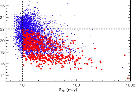
Figure 1: Left: r-band magnitude against 70 µm flux. Blue dots are all 70 µm detected sources with an optical counterpart in the LH and XMM-LSS. Filled red circles are the sources in the final 70 µm sample. The vertical line marks the 70 µm selection limit of 10 mJy and the horizontal line is at r = 22. Right: r-band magnitude against 160 µm flux. Blue dots are all 160 µm detected sources with an optical counterpart in the LH and XMM-LSS . Filled red circles are the sources in the final 160 µm sample. The vertical line marks the 160 µm selection limit of 60 mJy and the horizontal line is at r = 22.

In this paper we have used data from the latest release of the SWIRE photometric redshift catalogue of Rowan-Robinson et al. (2008). The catalogue contains photometric redshifts for over 1 million IR sources, estimated by combining the optical and IRAC 3.6 and 4.5 µm photometry to fit the observed SEDs with a combination of galaxy and AGN templates (Babbedge et al., 2004; Rowan-Robinson et al., 2005). Our analysis uses multiwavelength data from the XMM-LSS and Lockman Hole (LH) regions of the SWIRE survey.

2.2 Optical Data

Optical photometry is available for $>$ 70% of the SWIRE area in at least three of the U, g, r, i and Z photometric bands (Rowan-Robinson et al., 2008; Trichas et al., 2009). Spitzer-optical cross-identifications (XID) was carried out between the optical and the IRAC-24µm catalogues using a search radius of 1.5^′′ (Rowan-Robinson et al., 2005; Surace et al., 2005). The cross-identification process ensured that each SWIRE source only had one optical match. Completeness and reliability of the XID was investigated by Surace et al. (2005), which showed that essentially the Spitzer-optical XIDs are 100% complete. The requirement that the sources be detected at both 3.6 and 4.5 µm at S/N $\geq$ 5 appears to eliminate spurious sources effectively and give a high-reliability catalogueue (Rowan-Robinson et al., 2005; Surace et al., 2005).

The LH region centred on $\alpha$= $10^{\mathrm{h}}45^{\mathrm{m}}$, $\delta$ = $+57^{\mathrm{d}}59^{\mathrm{m}}$ covers $\sim$ 10.5 deg². Optical photometry is available covering 7.53 deg² in the g, r and i bands were obtained using the MOSAIC camera on the 4m-Mayall Telescope at Kitt Peak National Observatory (KPNO). The 5$\sigma$ limiting magnitudes (Vega) are 25.1, 24.4, and 23.7 in the three bands for point-like sources (Berta et al., 2007). U-band photometry is available in a smaller 1.24 deg² region to 5$\sigma$ limiting magnitude (Vega) of 24.1. The data reduction was performed with the Cambridge Astronomical Survey Unit (CASU) pipeline (Irwin & Lewis, 2001).

The XMM-LSS field centred on $\alpha$ = $02^{\mathrm{h}}21^{\mathrm{m}}$, $\delta$ = $-04^{\mathrm{d}}30^{\mathrm{m}}$ and covers 9.1 deg². Optical data is available for 6.97 deg² of XMM-LSS, which was observed as part of the Canada-France-Hawaii Telescope Legacy Survey (CFHTLS) in the u, g, r, i, and z bands to magnitude (Vega, 5$\sigma$ for a point like object) limits of: 24.9, 26.4, 25.5, 24.9 and 23.4 respectively. The photometry was taken from Pierre et al. (2007). In addition there is 10-band photometry (ugrizUBVRI) from the VIMOS VLT Deep Survey (VVDS) programme (Le Fèvre et al., 2004) covering 0.79 deg² and very deep 5-band photometry (BVRiz) in 1.12 deg² of the Subaru XMM Deep Survey (SXDS; Furusawa et al. 2008).

2.3 Sample Selection

Table 1: Summary of the sample selection used to study the 70 and 160 µm LFs.

Field	$\alpha$ (J2000)	$\delta$ (J2000)	Survey area	70 µm sources				160 µm sources
			(deg2)	$N_{\text{det}}$a	$N_{\text{sel}}$b	$N_{\text{sp}}$c	$N_{\text{sp}}$d	$N_{\text{det}}$a	$N_{\text{sel}}$b	$N_{\text{sp}}$c	$N_{\text{sp}}$e
							z $\leq 1.2$				z $\leq 0.5$
LH	$10^{\text{h}}45^{\text{m}}22^{\text{s}}$	$+57^{\text{d}}59^{\text{m}}05^{\text{s}}$	7.53	4046	2159	354	343	1276	584	166	157
XMM-LSS	$02^{\text{h}}21^{\text{m}}20^{\text{s}}$	$-04^{\text{d}}30^{\text{m}}00^{\text{s}}$	6.97	2358	1606	299	291	1604	739	81	64

^aNumber of sources detected; ^bNumber of sources selected using the selection criteria; ^cNumber of sources with spectroscopic redshift; ^dNumber of sources with spectroscopic redshift below 1.2; ^eNumber of sources with spectroscopic redshift below 0.5

To study the 70 and 160 µm LFs and their evolution, we select 1.) 70µm sources with r $<$ 22 mag and S${}_{70}>10$ mJy; and 2.) 160 µm sources with r $<$ 22 mag and S${}_{160}>$ 60 mJy. Furthermore, we require the sources to have measured spectroscopic redshifts. The adopted 70 and 160 µm flux limits correspond to 70% completeness of the SWIRE survey. The total IR LF is derived using the 70 µm sample.

The SWIRE photometric redshift catalogue of Rowan-Robinson et al. (2008) is the parent catalogue from which we select the 70 and 160 µm sources. In LH there are 4046 and 1276 sources detected at 70 and 160 µm respectively. Applying our selection criterion, 2159 70 µm and 584 160µm sources were selected. Spectroscopic redshifts are available for 354 70 µm and 166 160 µm sources, which were collated from literature.

In XMM-LSS, 2358 sources have 70 µm detections. We selected 1606 70µm sources, of which 299 have spectroscopic redshifts At 160 µm we found 1604 sources with 826 brighter than the flux limits stated above. We have spectroscopic redshifts for 81 160 µm sources. The spectroscopic redshifts in XMM-LSS were obtained from our spectroscopic follow-up programme conducted over 6 nights between November 2008-November 2009 at the WHT using the AF2/WYFFOS instrument. The details of the spectroscopic follow-up are presented in Patel et al. (2011).

We choose to construct the 70 µm and the total IR LFs in the redshift range $0<z\leq 1.2$ and the 160 µm LF in the redshift range $0<z\leq 0.5$. Thus, the final total sample of galaxies considered for the 70 µm and total IR LFs consists of 634 (343 in LH and 291 in XMM-LSS) objects and for the 160 µm LF consists of 221 (157 in LH and 64 in XMM-LSS) objects. We show in Figure 1 the r-band magnitude as a function of the 70 µm flux for all sources in the LH and XMM-LSS regions (filled blue circles) and the final spectroscopic sample (filled red circles).

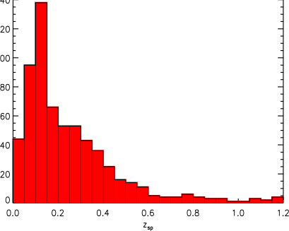
Figure 2: Spectroscopic redshift distribution for the final 70 µm sample. The 160 µm sample is a subset of the 70 µm sample restricted to $z<0.5$.

A summary of the parent catalogue and the final sample is presented in Table.1. We display the spectroscopic redshift distribution of the final 70 µm sample in Figure 2, while the final 160 µm sample has the same redshift distribution for $z\leq 0.5$, since all the 160 µm detected sources are also detected at 70 µm. The redshift distributions of the two fields is different because of large scale structures in the XMM-LSS field where the cluster distribution peaks around $z=0.3$ (Pacaud et al., 2007), which also corresponds to the peak in the redshift distribution of our sample.

3 INFRARED LUMINOSITIES

To determine the 70, 160 µm and total IR LFs from our sample, we need to derive the rest-frame 70 and 160 µm and the total IR luminosities. In order to do this, we model the SEDs for each source following the method described in Rowan-Robinson et al. (2005, 2008) used for the SWIRE photometric redshift catalogueue, using optical (at least 3 of the 5 optical U, g, r, i and Z bands) and IR photometry (Spitzer IRAC 3.6 - 8 µm and MIPS 24 - 160µm bands). The SED fitting follows a two-stage approach, by first fitting the optical to near-IR (U to 4.5µm) SED using the six galaxy and three AGN templates used by Rowan-Robinson et al. (2008).

We calculate the IR excess by subtracting the galaxy model fit from the 4.5 to 24µm data. We then fit the IR excess, 70 and 160µm (for 83 70µm sources) data points with the IR template of Rowan-Robinson et al. (2004, 2005, 2008). The IR templates are derived from radiative transfer models dependent on interstellar dust grains, the geometry and the density distribution of dust. The IR templates are: 1.) IR ’cirrus’: optically thin emission from interstellar dust illuminated by the interstellar radiation field; 2.) an M82 starburst; 3.) a more extreme Arp220-like starburst and 4.) an AGN dust torus. We also allow the sources to be fit by a mixture of: 1.) M82 starburst and cirrus, 2.) M82 starburst and AGN dust torus and 3.) Arp220 and AGN dust torus to properly represent the IR excess (Rowan-Robinson & Crawford, 1989; Rowan-Robinson et al., 2005).

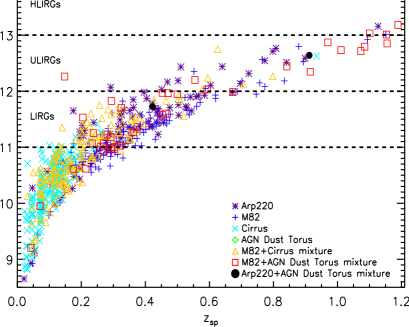
Figure 3: Total IR luminosity (L_IR) as a function of redshift for 70 µm sources with flux above 9 mJy. The horizontal lines mark the divisions for LIRGs (10${}^{11}\mathrm{L}_{\odot}<\mathrm{L_{IR}}<10^{12}\mathrm{L}_{\odot}$), ULIRGs (10${}^{12}\mathrm{L}_{\odot}<\mathrm{L_{IR}}<10^{13}\mathrm{L}_{\odot}$) and HLIRGs (L${}_{\mathrm{IR}}>10^{13}\mathrm{L}_{\odot}$).

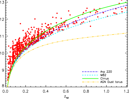
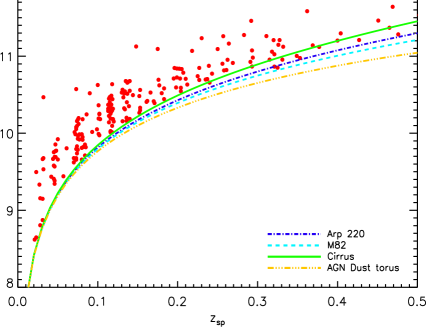
Figure 4: Left: Rest-frame 70 µm luminosity (L₇₀) as a function of redshift. The lines indicate as a function of redshift the 70 µm rest-frame luminosity corresponding to an observed 70 µm flux of 10 mJy with the 4 IR templates. Right: Rest-frame 160 µm luminosity (L₁₆₀) as a function of redshift. The lines indicate as a function of redshift the 160 µm rest-frame luminosity corresponding to an observed 160 µm flux of 60 mJy with the 4 IR templates.

From the SED fitting we find all but 12 of the $z<1.2$ sample are fit with a galaxy template in the optical, which implies that the contamination by AGNs is low in our sample. Thus, we choose to include all sources in our analysis and do not separate the galaxies from AGNs. We illustrate in Figure 3 the distribution of total IR luminosity (estimated by integrating the SED models between 8 - 1000 µm) as a function of redshift for the z $<$ 1.2 sample, with symbols representing the best fitting IR SED. The figure shows that in the IR the entire sample is dominated either by the starburst (Arp220 or M82-like) or the cirrus component, which is consistent with previous studies (Trichas et al., 2009; Symeonidis et al., 2010; Patel et al., 2011). Figure 3 also shows that most of the 70 µm sample are LIRGs and none of our sources have a pure AGN dust torus dominated IR SED.

We show in Figure 4 the rest-frame 70 µm luminosity (L₇₀) distribution as a function of redshift (left panel) and the rest-frame 160 µm luminosity (L₁₆₀) distribution as a function of redshift (right panel). The 70 and 160 µm luminosities were computed using K-corrections derived from the best fitting model templates. The uncertainty in the 70 and 160 µm and L_IR are typically 0.1 dex as stated in Patel et al. (2011). The SED model templates are also used to determine 1/$V_{\mathrm{max}}$, which is the volume corresponding to the maximum redshift at which a source could be detected by the survey given the optical and IR limits set in Section 2.3.

4 METHODOLOGY

In this section, we describe the methods used to determine the redshift evolution of the rest-frame 70, 160 µm and TIR LFs, derived using the spectroscopic sample described in Section 2.3 and using the optical and IR SED model of each source described in the previous section. The LF, denoted as $\Phi(L)~{}\text{d}\log{L}$, defines the number of objects per comoving volume within a luminosity range ${\log}L,{\log}L+\text{d}\log{L}$. We construct the 70 µm and total IR LFs in the redshift bins [0–0.2], [0.2–0.4], [0.4–0.8] and [0.8–1.2] and the 160 µm LF in the redshift bins [0–0.2] and [0.2–0.5] using the 1/$V_{\mathrm{max}}$ method (Schmidt, 1968; Avni & Bahcall, 1980). We also develop a Bayesian method to study the evolution of the 70 and 160 µm and the TIR LFs. In our LF estimation methods we accurately model the different completeness and selection effects affecting our data. The selection and incompleteness functions are described in Section 4.1 and the binned and parametric LF methods are discussed in Section 4.2 and Section 4.3 respectively.

4.1 Selection and Incompleteness Function

The data set we have used to estimate the FIR LFs was selected by imposing multivariate flux limits to determine whether a source is included in our sample. In addition we require each of the sources to then have a spectroscopic redshift. Here we use the 70 µm LF selection functions as an example but the general procedure is the same for the total IR and 160 µm LFs.

The 70 µm LF is calculated by selecting sources in the SWIRE catalogue that have S${}_{70}>$ 10 mJy, $r<$ 22 mag and measured spectroscopic redshift. Therefore our first selection function considers the probability that a source of a given 70 µm flux (which is a function of luminosity, $L$, and redshift $z$) is detected by the survey. This is denoted as $p$(det$|L,z$), and has been determined by Vaccari et al. (in preparation) for each field in the SWIRE survey using Monte Carlo simulations. The second selection function considers the probability that a given 70 µm source with luminosity, $L$ at redshift $z$ is associated with an optical counterpart at $r<$ 22 mag and is defined as $p(r<22|L,z$). This was quantified by taking the SWIRE catalogue and constructing a source count distribution for all sources detected at 70 µm and then constructing a similar source count distribution for all 70 µm sources with $r<$ 22 mag and the ratio is used to estimate $p(r<22|L,z$).

Finally, we take into account the probability that a given source to be characterised with a spectroscopic redshift. The spectroscopic incompleteness is primarily determined by the $r$ band magnitude and therefore they are added as weights in the computation of the LF (see Section 4.2 and Section 4.3). We define the weights, $w$, as the inverse of the spectroscopic completeness. The spectroscopic completeness is determined by constructing the source distribution for all sources with a measured spectroscopic redshift as a function of $r$ magnitude and dividing this by the source count distribution for all 70 µm sources with S${}_{70}>10$ mJy and $r<22$ as a function of $r$ magnitude.

and total IR LFs. The selection function, defined as $p$(selected$|L,z$), are combinations of the two selection functions:

$$p\mathrm{(selected}|L,z)=p\mathrm{(det}|L,z)p(r<22|L,z)$$ (1)

The selection function and the spectroscopic incompleteness were used to modify the LF methods discussed in the following section.

4.2 Binned Estimates

We use the 1/$V_{\mathrm{max}}$ method as the binned estimate which has the advantage that it allows direct computation of the LF from the data, without any parametric dependence or model assumption. We divided the sample into redshift bins selected to ensure adequate numbers of galaxies in each bin. For each redshift bin, the LF is given by:

$$\Phi(L)\mathrm{d}\log{L}=\left(\displaystyle\sum_{i}w_{i}\times\frac{1}{V_{\mathrm{max},i}}\right),$$ (2)

where $V_{\mathrm{max},i}$ is the comoving volume out to which the ith galaxy could be observed, $w_{i}$ is the inverse of the spectroscopic incompleteness of the ith galaxy. The comoving volume, $V_{\mathrm{max},i}$ is:

$$V_{\mathrm{max},i}=\int_{z_{\mathrm{min}}}^{z_{\mathrm{max},i}}p\mathrm{(selected|}L_{i},z)\frac{\mathrm{d}V}{\mathrm{d}z}\mathrm{d}z,$$ (3)

where d$V$/d$z$ is the differential comoving element per unit solid angle (Hogg, 1999). Here $z_{\mathrm{max},i}$ corresponds to the maximum redshift at which the source could be detected by the survey given the optical flux limit ($r<22$) or the IR flux limits (S${}_{70}>$ 10 mJy or S${}_{160}>$ 60 mJy) and $z_{\mathrm{min}}$ is the lower limit of the redshift bin. $z_{\mathrm{max},i}$ was determined by using the optical/NIR and IR SED model of each source. The volume element integral in the LF calculation was weighted by the selection function to correct for the selection biases that are inherent in the spectroscopic catalogueue. The IR SED models described in Section 3 are used in computing the selection function.

The associated rms error is given by:

$$\sigma_{\Phi(L)}=\sqrt{\left(\displaystyle\sum_{i}w_{i}^{2}\times\frac{1}{V_{\mathrm{max},i}^{2}}\right)},$$ (4)

In order to accurately determine the uncertainty in the LF error we use Monte Carlo bootstrapping analysis to randomly resample the final spectroscopic catalogueue to generate 1000 realisations; each of these is analysed as described above and the root mean square (RMS) of the results is quoted as the error.

4.3 Parametric Bayesian Method

We use a Bayesian approach to determine the parametric LF, which requires prior knowledge of the appropriate functional form of the LF. As is the case for maximum likelihood (ML) methods (Sandage et al., 1979; Marshall et al., 1983) the parametric LF has the advantage over the 1/$V_{\mathrm{max}}$ method in that it is insensitive to any local clustering effect whereas the 1/$V_{\mathrm{max}}$ LF assumes a uniform number density throughout the observed volume and therefore is vulnerable to density inhomogeneities present in the survey (Wang & Rowan-Robinson, 2010). The advantage of using a Bayesian method to estimate the LF parameters over ML methods is that ML methods do not provide an estimate of the LF normalisation, which is often chosen to make the expected number of sources detected in a survey equal to the actual number of sourced detected. In addition, the confidence intervals on the LF parameters are derived assuming they have a Gaussian distribution which is not necessarily a good approximation for small sample sizes (Kelly et al., 2008).

In order to carry out a Bayesian analysis we first need to define the likelihood function, $p(\{d\}|\{\theta\}$), which is the probability of observing the data, $\{d\}$, for a given LF model, that is described by some parameters $\{\theta\}$. To do this we first define the probability of finding a source of a specific luminosity $L_{i}$ in the range $\log{L},{\log}{L}+\text{d}\log{L}$ at a redshift $z_{i}$ in the range $z,z+\mathrm{d}z$ as:

$$p(L,z|\{\theta\})=\frac{\Phi(L,z|\{\theta\})p(\text{selected}|L,z)}{\lambda}\frac{\mathrm{d}V}{\mathrm{d}z},$$ (5)

where $\lambda$ is the expected number of sources and is determined by:

$$\lambda=\displaystyle\sum_{\mathrm{fields}}\iint\Phi(L,z|\{\theta\})p\mathrm{(selected|}L,z)\mathrm{d}\log{L}\frac{\mathrm{d}V}{\mathrm{d}z}\mathrm{d}z$$ (6)

The sum is taken over the fields present in our survey and the integrals are taken over all possible values of redshifts and luminosities.

We now write the likelihood function as the probability of observing $N$ objects, each with $L_{i}$ and $z_{i}$, drawn from the model LF as:

$$p(\{d\}|\{\theta\}) =p(N,\{L_{i},z_{i}\}|\{\theta\})$$

$$=p(N|\{\theta\})p(\{L_{i},z_{i}\}|\{\theta\})$$ (7)

where $p(N|\{\theta\})$ is the probability of observing $N$ objects given the model LF and $p(\{L_{i},z_{i}\}|\{\theta\})$ is the likelihood of observing a set of $L_{i}$ and $z_{i}$ given the model LF. We assume that the number of sources detected follows a Poisson distribution, where the expected number of detectable sources, $\lambda$, is given by Equation 6. Thus the likelihood function is written as:

$$p(N,\{L_{i},z_{i}\}|\{\theta\}) =\frac{\lambda^{N}e^{-\lambda}}{N!}\displaystyle\prod_{i=1}^{N}p(L_{i},z_{i}|\{\theta\})$$ (8)

$$=\frac{\lambda^{N}e^{-\lambda}}{N!}\;\;\times$$

$$\displaystyle\prod_{i=1}^{N}\frac{\Phi(L,z|\{\theta\})p\mathrm{(selected|}L,z)}{\lambda}\frac{\mathrm{d}V}{\mathrm{d}z}$$ (9)

We further modify the likelihood function by including the spectroscopic incompleteness by introducing a weighting factor, $w/\langle{w}\rangle$, for each object (see Zucca et al., 1994; Ilbert et al., 2005; Aird et al., 2008). The weights, added as exponents of the individual source likelihoods $p(\{L_{i},z_{i}\}|\{\theta\})$ artificially reduce the size of error estimates. Therefore they are balanced by the average weight ($\langle{w}\rangle$) which do not effect the best fitting parameters (Aird et al., 2008). Furthermore, $N$, the total number of objects is now $\sum{w_{i}}$, which gives the effective number of sources corrected for the spectroscopic incompleteness. Therefore the likelihood function in Equation 9 is:

$$p(N,\{L_{i},z_{i}\}|\{\theta\}) \propto\lambda^{\sum{w_{i}}}e^{-\lambda}\;\>\times$$

$$\displaystyle\prod_{i=1}^{N}\left\{\frac{\Phi(L,z|\{\theta\})p\mathrm{(selected|}L,z)}{\lambda}\frac{\mathrm{d}V}{\mathrm{d}z}\right\}^{\frac{w_{i}}{\langle{w}\rangle}}$$

Note that in the absence of the spectroscopic incompleteness weights, $w_{i}$, Equation LABEL:eq:lhfunc reduces to the form presented in Marshall et al. (1983).

We perform Bayesian inference by combining the LF with a prior probability distribution, $p(\{\theta\})$ to compute the posterior probability distribution, $p(\{\theta\}|\{d\})$, given by Bayes’ theorem:

$$p(\{\theta\}|\{d\})=\frac{p(\{d\}|\{\theta\})p(\{\theta\})}{\int{p(\{d\}|\{\theta\})p(\{\theta\})}d\theta},$$ (11)

where the denominator is the Bayesian evidence and is determined by integrating the likelihood over the prior parameter space.

For parameter inference, the Bayesian evidence serves to normalise the posterior distribution and is vital for Bayesian model comparison. Calculating the Bayesian evidence is computationally expensive since it involves integration over $n$-dimensions for an $n$ parameter LF model. Therefore we use standard Markov chain Monte Carlo (MCMC) methods to perform a random walk through the parameter space to obtain random samples from the posterior distribution. We employed the Metropolis-Hastings algorithm (Metropolis et al., 1953; Hastings, 1970), in which a proposal distribution is used to guide the variation of the parameters. The algorithm uses a proposal distribution which depends on the current state to generate a new proposal sample. We accept a step if the probability of the model given the new parameter values is higher and also at random intervals when the probability is lower in order to allow the fit to proceed downhill to avoid local minima (Ptak et al., 2007; Kelly et al., 2008).

We assume a flat prior distribution for each parameter and ignoring the normalising factor, the Bayesian evidence, the posterior distribution for each parameter is then given by:

$$p(\{\theta\}|\{d\})\propto p(\{d\}|\{\theta\})$$ (12)

We produce three chains for each analysis of at least $2\times 10^{6}$ iterations and adjust the parameter step sizes to achieve an acceptance ratio in the range 0.3 - 0.5. Finally we calculated the convergence $R$ statistic from Gelman et al. (2004), which should be $\leq 1.2$ if the chain has converged. For all the parameters the $R$ value was $<1.1$.

4.3.1 Luminosity Function Models

The first IR LF constructed from IRAS observations showed an excess in the number of galaxies at the high luminosity end (Soifer et al., 1987) from the value expected from the Schechter function (Schechter, 1976). Soifer et al. (1987) fit a double power-law model to the IRAS 60 µm LF which is adopted in our work. We use a continuous double power-law model given by:

$$\Phi(L|\{\theta\})=\phi^{\ast}\left[\left(\frac{L}{L^{\ast}}\right)^{\alpha}+\left(\frac{L}{L^{\ast}}\right)^{\beta}\right]^{-1}$$ (13)

Alternatively Saunders et al. (1990) fit the IRAS 60 µm LF with a combination of a power-law and log-normal LF model:

$$\Phi(L|\{\theta\})=\phi^{\ast}\left(\frac{L}{L^{\ast}}\right)^{(1-\alpha)}\exp\left[-\frac{1}{2\sigma^{2}}\log^{2}\left(1+\frac{L}{L^{\ast}}\right)\right].$$ (14)

In both models, $L^{\ast}$ is the characteristic luminosity, $\phi^{\ast}$ is the LF normalisation and $\alpha$ is the power-law of the faint-end of the LF. $\beta$ in Equation 13 is the power-law index of the bright-end of the LF and $\sigma$ in Equation 14 gives the range over which the LF drops off.

We estimate the parameters of the double power-law model, defined model 1, and the power-law and log-normal model, defined model 2. Uniform prior probability for all parameters were assumed with limits as follows: $-1\leq\alpha\leq 2$, $0\leq\sigma\leq 1$, $1\leq\beta\leq 6$, $8\leq\log{L^{\ast}}\leq 12$ and $-1\leq\log{\phi^{\ast}}\leq-4$.

4.3.2 Luminosity Function Evolution Model

Several studies (see Le Floc’h et al., 2005; Pérez-González et al., 2005; Caputi et al., 2007; Magnelli et al., 2009; Rujopakarn et al., 2010) of the IR luminosity functions, mainly at 24 µm have shown that out to $z\sim 1.2$, the while the luminosity and the number density of the LF evolves, the shape remains the same, that is $\alpha$, $\beta$ (in Equation 13) or $\sigma$ (in Equation 14) do not change. We parameterize the evolution of the FIR LFs in luminosity only:

$$\Phi(L,z|\{\theta\})=\Phi\left[\frac{L}{f(z)}|\{\theta\}\right],$$ (15)

where $f(z)=(1+z)^{\text{\hbox{$\alpha_{\textsc{l}}$}}}$. Therefore in addition to the parameters listed in the previous section, $\alpha_{\textsc{l}}$, the luminosity evolution power-law index was also constrained. Uniform prior probability distributions were assumed for $\alpha_{\textsc{l}}$ with limits: $1\leq\text{\hbox{$\alpha_{\textsc{l}}$}}\leq 7$. Thus, for each LF model (double power-law and power-law and log-normal) five parameters were estimated.

5 RESULTS

In this section, we present our determinations of the FIR LF and compare them to previous studies. We construct the rest-frame 70 µm and the TIR LFs in redshift range $0<z\leq 1.2$ and the rest-frame 160 µm LF in the redshift range $0<z\leq 0.5$. Finally using the TIR LF we derive the co-moving IR luminosity density and the cosmic star formation rate density as a function of redshift in the range $0<z\leq 1.2$.

5.1 Evolution of the Rest-frame 70 ${\mu}$m Luminosity Function

In Figure 5, we show the rest-frame 70 µm LF constructed using the 1/$V_{\mathrm{max}}$ (black filled circles) and the parametric Bayesian (solid red and blue lines) methods described in Section 4. The parametric LFs are displayed using the best-fit (posterior mode) parameters given in Table 3. We also display the $z=0$ LF (dashed red and blue lines), which shows the rapid evolution of the 70 µm LF, when compared with the binned and evolved parametric LFs. The parametric 70 µm LF uses k-correction according to the M82 starburst SED.

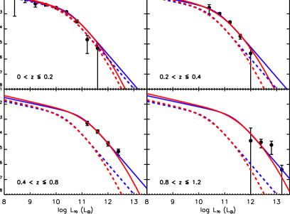
Figure 5: 70 µm LF split into redshift bins $0<z\leq 0.2$, $0.2<z\leq 0.4$, $0.4<z\leq 0.8$ and $0.8<z\leq 1.2$. The 1/$V_{\mathrm{max}}$ LF is shown as filled black circles, the solid blue line is the double power-law LF and the solid red line is the power-law and log-normal LF. The parametric LFs are displayed using the best-fit parameters listed in Table 3 and evaluated at $z=0.1$, 0.3, 0.6 and 1. The dashed red and blue lines are the $z=0$ LFs.

	$\log\Phi$ (Mpc-3)
$\log~{}L_{70}$ (L⊙)	$0<{z}\leq 0.2$	$0.2<{z}\leq 0.4$	$0.4<{z}\leq 0.8$	$0.8<{z}\leq 1.2$
8.4	$-1.96^{+0.29}_{-1.20}$
8.8	$-1.99^{+0.16}_{-0.27}$
9.2	$-2.33^{+0.15}_{-0.22}$
9.6	$-2.39^{+0.08}_{-0.10}$
10.0	$-2.59^{+0.06}_{-0.07}$
10.4	$-2.87^{+0.05}_{-0.06}$	$-2.59^{+0.20}_{-0.40}$
10.8	$-3.49^{+0.09}_{-0.11}$	$-2.99^{+0.07}_{-0.08}$
11.2	$-4.71^{+0.27}_{-0.92}$	$-3.55^{+0.07}_{-0.08}$	$-3.25^{+0.12}_{-0.16}$
11.6	$-5.28^{+0.31}_{-5.28}$	$-4.49^{+0.13}_{-0.19}$	$-3.80^{+0.10}_{-0.14}$
12.0		$-5.62^{+0.34}_{-5.62}$	$-4.60^{+0.13}_{-0.18}$	$-4.43^{+0.85}_{-4.43}$
12.4			$-5.14^{+0.16}_{-0.25}$	$-4.52^{+0.20}_{-0.37}$
12.8				$-4.70^{+0.25}_{-0.63}$
13.2				$-6.36^{+0.30}_{-6.36}$

Table 2: 1/$V_{\mathrm{max}}$ 70 µm luminosity function values.

	70 µm LF		160 µm LF		Total IR LF
Parameter	(a)	(b)	(a)	(b)	(a)	(b)
$\log L^{\ast}$ (L⊙)	$10.35^{+0.12}_{-0.09}$	$9.53^{+0.10}_{-0.11}$	$10.21^{+0.10}_{-0.08}$	$9.85^{+0.18}_{-0.45}$	$10.61^{+0.05}_{-0.13}$	$9.71^{+0.19}_{-0.19}$
$\alpha$	$0.37^{+0.10}_{-0.13}$	$1.40^{+0.10}_{-0.09}$	$0.40^{+0.17}_{-0.21}$	$1.07^{+0.14}_{-0.58}$	$0.34^{+0.10}_{-0.12}$	$1.38^{+0.09}_{-0.12}$
$\beta$	$2.00^{+0.13}_{-0.12}$	–	$3.79^{+0.36}_{-0.23}$	–	$2.09^{+0.14}_{-0.10}$	–
$\sigma$	–	$0.66^{+0.07}_{-0.03}$	–	$0.29^{+0.08}_{-0.05}$	–	$0.63^{+0.06}_{-0.04}$
$\log\phi^{\ast}$ (Mpc-3)	$-2.68^{+0.09}_{-0.14}$	$-2.32^{+0.14}_{-0.06}$	$-2.84^{+0.15}_{-0.11}$	$-2.43^{+0.11}_{-0.16}$	$-2.68^{+0.12}_{-0.10}$	$-2.26^{+0.11}_{-0.12}$
$\alpha_{\textsc{l}}$	$3.39^{+0.12}_{-0.22}$	$3.41^{+0.18}_{-0.25}$	$5.73^{+0.30}_{-0.62}$	$5.53^{+0.28}_{-0.23}$	$3.82^{+0.24}_{-0.20}$	$3.82^{+0.25}_{-0.16}$

Table 3: Best-fitting parameters for of the 70 and 160 µm and TIR LFs determined using the parametric Bayesian method. The errors include 68% of the posterior probability. (a) double power-law LF model and (b) power-law and log-Gaussian LF model.

Examination of the binned and parametric LFs in Figure 5, shows excellent agreement across all redshift bins. Comparison of the two LF models indicates that they are almost identical except at the brightest luminosities (L₇₀ $>10^{12}$ L_⊙), where the power-law and log-normal LF model has a rapid drop off when compared with the double power-law model. However, since there are no data points at these brightest luminosities, both LF models are a good description of the evolution of the 70 µm LF. The shape of the faint-end of the LF is also consistent; $\alpha=0.37^{+0.10}_{-0.13}$ for model 1 and; $\alpha=1.40^{+0.10}_{-0.09}$ for model 2 as observed in the $0<z\leq 0.2$ redshift bin. The luminosity evolution parameter, $\alpha_{\textsc{l}}$, which shows that the characteristic luminosity evolves rapidly as a function of redshift is almost identical for the two LF models ($\alpha_{\textsc{l}}$ $=3.39^{+0.12}_{-0.22}$ and $\alpha_{\textsc{l}}$ $=3.41^{+0.18}_{-0.25}$ for model 1 and 2 respectively). The best fit evolutionary parameter is consistent with studies performed at several IR wavelengths, in particular at 24 µm, which find strong luminosity evolution with $\text{\hbox{$\alpha_{\textsc{l}}$}}=3-5$ (see Le Floc’h et al., 2005; Babbedge et al., 2006; Magnelli et al., 2009; Rujopakarn et al., 2010). We find that both parametric models can describe the evolution of the 70 µm LF.

We shown in Figure 6, the SWIRE 70 µm local luminosity function (LLF) constructed in the redshift bin $0<z\leq 0.2$, is compared to the bandpass corrected (assuming an M82 starburst SED) IRAS 60 µm LFs determined by Saunders et al. (1990) (filled blue square), Takeuchi et al. (2003) (solid red line) and Wang & Rowan-Robinson (2010) (solid green line). Comparison of the LFs shows that the overall shape of the parametric and binned 70 µm LF is well matched to the bandpass corrected 60 µm LFs. Takeuchi et al. (2003) IRAS 60 µm LF report, $\log L^{\ast}$ (L_⊙) $=9.07\pm 0.09$, $\alpha=1.23\pm 0.04$, $\sigma=0.72\pm 0.01$ and $\log\phi^{\ast}$ (Mpc^-3) $=-2.05\pm 0.05$ while Wang & Rowan-Robinson (2010) determine, $\log L^{\ast}$ (L_⊙) $=9.10$, $\alpha=1.29$, $\sigma=0.72$ and $\log\phi^{\ast}$ (Mpc^-3) $=-2.05$. At the faint-end, the 70 µm LF is steeper with $\alpha=1.40^{+0.10}_{-0.09}$ for model 2, while $\sigma=0.66^{+0.07}_{-0.03}$, in excellent agreement with the value determined from IRAS surveys.

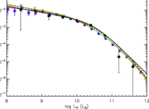
Figure 6: The LLF ($0<z\leq 0.2$) at 70 µm determined using 1/$V_{\mathrm{max}}$ (filled black circles) and the parametric Bayesian method (solid and dashed black lines) evaluated at $z=0.1$. The solid black line is the double-power law model and the dashed black line is the power-law and log-normal model. Binned IRAS 60 µm LF from Saunders et al. (1990) is shown in filled blue squares and the parametric 60 µm LF from Takeuchi et al. (2003) (solid red line) and Wang & Rowan-Robinson (2010) (solid green line) are corrected for the bandpass differences assuming an M82 type starburst SED.

We have used the k-correction given by the M82 starburst SED template in order to determine $p(\mbox{selected}|L,z)$ in the likelihood function because a large fraction of the 70 µm population are fit with this template (see Section 3 and Figure 3). Although using a k-correction of a pure Arp220 starburst or a pure cirrus SED template results in different values for $\alpha_{\textsc{l}}$, we still find that the 70 µm LF evolves rapidly in luminosity ($\alpha_{\textsc{l}}$ $>$ 3). Studying the LF evolution of each SED component will be further investigated in future studies (see Section 6.3).

5.2 Evolution of the Rest-frame 160 ${\mu}$m Luminosity Function

The rest-frame 160 µm LF constructed using the 1/$V_{\mathrm{max}}$ (filled black circles) and the parametric Bayesian (solid red and blue lines) methods is shown in Figure 7. The parametric LFs are displayed using the best-fit parameters given in Table 3 and the 1/$V_{\mathrm{max}}$ values are listed in Table 4. The $z=0$ LF is also displayed (dashed red and blue lines), which show the rapid evolution of the 160 µm LF, when compared with the binned and the evolved parametric LFs. The parametric Bayesian 160 µm LF was calculated using a k-correction given by a mixture of M82 starburst (50%) and cirrus template (50%).

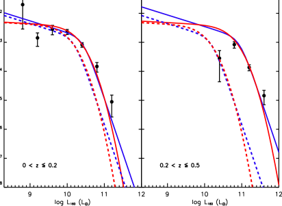
Figure 7: 160 µm LF split into redshift bins $0<z\leq 0.2$ and $0.2<z\leq 0.5$. The 1/$V_{\mathrm{max}}$ LF is shown as filled black circles, the solid blue line is the double power-law LF and the solid red line is the power-law and log-normal LF. The parametric LFs are displayed using the best-fit parameters listed in Table 3 and evaluated at $z=0.1$ and 0.5. The dashed red and blue lines are the $z=0$ LFs.

	$\log\Phi$ (Mpc-3)
$\log{L_{160}}$ (L⊙)	$0<{z}\leq 0.2$	$0.2<{z}\leq 0.5$
8.8	$-1.70^{+0.26}_{-0.84}$
9.2	$-2.85^{+0.17}_{-0.29}$
9.6	$-2.55^{+0.13}_{-0.19}$
10.0	$-2.63^{+0.08}_{-0.10}$
10.4	$-3.08^{+0.07}_{-0.09}$	$-3.55^{+0.27}_{-0.81}$
10.8	$-3.83^{+0.13}_{-0.19}$	$-3.08^{+0.10}_{-0.12}$
11.2	$-5.05^{+0.23}_{-0.52}$	$-3.87^{+0.09}_{-0.11}$
11.6		$-4.84^{+0.18}_{-0.31}$

Table 4: The 1/$V_{\mathrm{max}}$ 160 $\mu$m LF values.

The binned and parametric LFs shown in Figure 7 are consistent with each other except at L₁₆₀ $>10^{11}$ L_⊙ where both the parametric LFs show a faster drop-off. In fact the double power law LF model shows a much better agreement with the 1/$V_{\mathrm{max}}$ LF in both redshift bins at L₁₆₀ $>10^{11}$ L_⊙ implying that the double power law LF model may be a better description of FIR LFs. The 160 µm LF evolves in luminosity with $\alpha_{\textsc{l}}$ $=5.73^{+0.29}_{-0.62}$ for model 1 and $\alpha_{\textsc{l}}$ $=5.53^{+0.28}_{-0.23}$ for model 2, which is stronger than the value found for the evolution of the 70 µm LF or from Spitzer 24 µm studies (see Le Floc’h et al., 2005; Babbedge et al., 2006; Magnelli et al., 2009; Rujopakarn et al., 2010). Takeuchi et al. (2006) however find that the ISO 170 µm LF evolves with $\alpha_{\textsc{l}}$ $=5.0^{+2.3}_{-0.5}$, being entirely consistent with the evolution of 160 µm LF. Recently, Dye et al. (2010) used data from the H-ATLAS survey to find that the rest-frame 250 µm luminosity density evolves at a rate proportional to $(1+z)^{7.1^{+2.1}_{-1.4}}$ to $z\simeq 0.2$ in agreement with the evolution of 160 and 170 µm LFs.

Our results show that the 160 µm LF evolves more rapidly than the 70 µm LF suggesting that ‘cooler’ galaxies evolve more rapidly than ‘warmer’ galaxies (the 160 µm LF was determined using the k-correction given by a mixture of M82 starburst and cirrus template whereas the 70 µm LF was determined using the k-correction given by an M82 starburst template). This is in keeping with the work of Symeonidis et al. (2011) who find that ‘cold’ galaxies evolve more rapidly than ‘warmer’ galaxies over a period of $0.1<z<1$. Dunne et al. (2011) have shown that the evolution of the 250 µm LF out to $z=0.5$ is driven in part by evolution in the dust mass and an increase in the luminosity or space density of cooler galaxies. They conclude that the evolution of the dust mass points to an enhanced supply of gas for star formation at earlier cosmic epochs.

We compare in Figure 8 our 160 µm LLF with the ISO 170 µm LF from Takeuchi et al. (2006) constructed using 55 galaxies at $z<0.3$. The 170 µm binned LF shows a reasonable agreement within the error bars with the 160 µm LF except at L₁₆₀ $\lesssim 10^{10}$ L_⊙ where there is a significant discrepancy between the two LFs, which is most likely due to the small number of objects in the 170 µm sample. Takeuchi et al. (2006) use the power-law and log-normal LF model and conclude that the parametric form (solid red line in Figure 8) underestimates the bright end of the LF, similar to the findings reported here. The combination of these results indicates that the double power-law model is the favoured analytic form for FIR LFs.

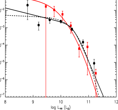
Figure 8: The LLF ($0<z\leq 0.2$) 160 µm LF determined using 1/$V_{\mathrm{max}}$ (filled black circles) and the parametric Bayesian method (solid and dashed black lines) evaluated at $z=0.1$. The solid black line represents the double-power law model and the dashed black line is the power-law and Gaussian model.The parametric (red solid line) and non-parametric (red filled squares) ISO 170 µm LFs from Takeuchi et al. (2006) are shown for comparison.

5.3 Total Infrared Luminosity Function

In this section, we compute the total IR luminosity function of galaxies using the observed 70 µm data. The total IR luminosity of a star forming galaxy provides a direct estimate of current star formation activity because the IR emission is the reprocessed UV/optical radiation produced by young stars. L_IR can be converted to SFR using the relationship provided by Kennicutt (1998):

$$\mathrm{SFR}\>(\mathrm{M_{\odot}\>yr^{-1}})=1.72\times 10^{-10}~{}\mathrm{L_{IR}}\>\mathrm{L_{\odot}},$$ (16)

where L_IR is estimated by integrating for each source the best fit SED in the interval $8-1000\mu$m (see Section 3). We can then use Equation 16 and the total IR LF to derive an estimate of the IR comoving energy density and the cosmic star formation rate density (CSFRD) up to z $\sim$ 1.2 and compare these results with other CSFRD calibrators.

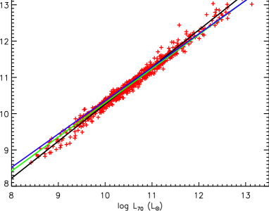
Figure 9: Correlation between rest frame 70 µm luminosity ($\log$ L₇₀) and total IR luminosity ($\log$ L_IR). The black solid line is our linear relationship determined using a Bayesian linear regression method. We also show for comparison the linear relation from Symeonidis et al. (2008) (blue solid line) and Bavouzet et al. (2008) (green solid line).

Previous studies of the the total IR LFs have largely been conducted at MIR wavelengths, with the greatest progress made at the Spitzer 24 µm band where MIPS is most sensitive (see. Le Floc’h et al., 2005; Pérez-González et al., 2005; Babbedge et al., 2006; Caputi et al., 2007; Béthermin et al., 2010b; Rodighiero et al., 2010). The work presented here follows a similar approach to others in the literature, which relies on the conversion of $\mbox{L}_{\nu}$ to L_IR, usually calibrated using SED templates of local IR galaxies (Chary & Elbaz, 2001) or semi-empirical SEDs (Dale & Helou, 2002; Lagache et al., 2003). Several authors (Elbaz et al., 2002; Appleton et al., 2004) and in paritucular Bavouzet et al. (2008), have shown that the extrapolation of the local $\mbox{L}_{\nu}-\mathrm{L_{IR}}$ remains reliable up to $z=1.1$ for LIRGs and $z\sim$ 2 for ULIRGs. Furthermore, the wavelength closest to the peak of far-IR emission provides the most accurate estimator of L_IR (Bavouzet et al., 2008).

We use the SED templates of Rowan-Robinson et al. (2004, 2005, 2008) and therefore to check the consistency of our $\mbox{L}_{70}-\mathrm{L_{IR}}$ correlation, we compared our results with those of Bavouzet et al. (2008) and Symeonidis et al. (2008). In Figure 9 we show the relationship between $\log$ L₇₀ and $\log$ L_IR for all sources at $z<1.2$ in our sample (black solid line) with the relations of Bavouzet et al. (2008) (green solid line) and Symeonidis et al. (2008) (blue solid line). The three correlations show excellent agreement with a mean scatter of $\sim 0.1$ dex between our correlation and the other two in the luminosity range $9.5\lesssim\log\text{L}_{70}\lesssim 12.5$. Therefore we choose to use our $\mbox{L}_{70}-\mathrm{L_{IR}}$ correlation in constructing the total IR LF.

To calculate the 1/$V_{\mathrm{max}}$ LF, we follow the same method as described in Section 4.2 and use the 70 µm selection function for each source. For the Bayesian analysis we use our linear relationship between $\mbox{L}_{70}-\mathrm{L_{IR}}$ to convert L_IR to L₇₀ to determine the selection function $p(\mathrm{selected}|L,z)$ in the likelihood function. Thus, the Bayesian analysis is dependent on the values of the linear relationship shown in Figure 9. We perform a test by estimating the parameters of the local total IR LF using the correlations of Bavouzet et al. (2008) and Symeonidis et al. (2008) and found all parameters to be almost identical.

5.3.1 Evolution of the Total Infrared Luminosity Function

In Figure 10, we display the TIR LF constructed using the 1/$V_{\mathrm{max}}$ (filled black circles) and the parametric Bayesian (solid black line) methods. The parametric LFs are displayed using the best-fit parameters given in Table 3 and the 1/$V_{\mathrm{max}}$ values are listed in Table 5. The $z=0$ LF is also displayed (dashed black line), which show the rapid evolution of the TIR LF, when compared with the binned and the evolved parametric LFs. The parametric TIR LF was calculated using the k-correction given by the M82 starburst SED.

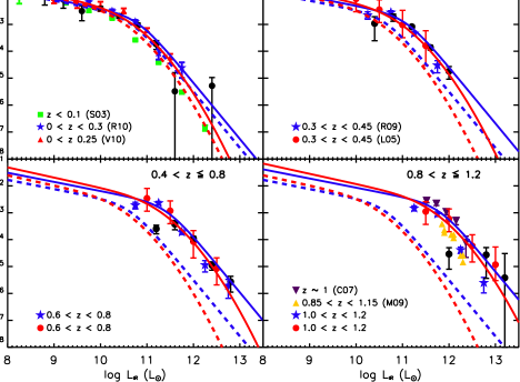
Figure 10: TIR LF split into redshift bins $0<z\leq 0.2$, $0.2<z\leq 0.4$, $0.4<z\leq 0.8$ and $0.8<z\leq 1.2$. Filled black circles are the 1/$V_{\mathrm{max}}$ estimates and the black solid line is the parametric Bayesian LF displayed using the best-fit parameters given in Table 3 at $z=0.1$, 0.3, 0.6 and 1. Filled red filled circles are from Le Floc’h et al. (2005), filled purple upside down triangles are from Caputi et al. (2007), filled orange filled upside down triangles are from Magnelli et al. (2009) and filled blue filled stars are from Rodighiero et al. (2010). The $z=0$ LF is shown in each panel (black dashed line).

Comparison of the 1/$V_{\mathrm{max}}$ and parametric LFs in Figure 10 shows good agreement across all redshift bins for both LF models. We find the evolution of the TIR LF is independent of the two LF models used ($\alpha_{\textsc{l}}$ $=3.82^{+0.24}_{-0.20}$ for model 1 and $\alpha_{\textsc{l}}$ $=3.82^{+0.25}_{-0.16}$ for model 2), similar to the results of the 70 and 160 µm LFs. Thus the choice of the LF model does not affect the conclusion that the TIR LF which shows strong evolution in luminosity. The global evolution parameter of the TIR LF is consistent with values determined by previous studies, which typically find $\alpha_{\textsc{l}}$ $\sim 3.5\pm 0.5$ (Caputi et al., 2007; Le Floc’h et al., 2005; Magnelli et al., 2009) out to $z\sim 1$. In Figure 10, the TIR LFs are compared with literature values in the higher redshift bins. As shown in this figure, our TIR LF shown is broadly consistent with the published results in the redshift bins $[0-0.2]$, $[0.2-0.4]$ and $[0.4-0.8]$. We find excellent agreement when we compare our 1/$V_{\mathrm{max}}$ LF in the redshift bins $[0.3-0.45]$ and $[0.6-0.8]$ to the values of Le Floc’h et al. (2005) and Rodighiero et al. (2010) in the same redshift bins. In the highest redshift bin, $[0.8-1.2]$, our TIR LF shows a good agreement with the LF determined by Le Floc’h et al. (2005). The SWIRE TIR LF however shows differences with the values of Caputi et al. (2007); Magnelli et al. (2009) and Rodighiero et al. (2010). Magnelli et al. (2009) investigated the difference between their and the Le Floc’h et al. (2005) LF values and found that the difference appears to be because of the choice of SED library and the correlation used to convert $L_{\lambda}$ to L_IR. Thus, this may also be the reason for the difference seen in the comparison of this work with theirs. Therefore although the 1/$V_{\mathrm{max}}$ LF values in the highest redshift bins are less robust, the parametric TIR LF and its evolution conforms to results that have been determined previously.

In Figure 11, we compare our local TIR LF with the IRAS revised bright galaxy sample (BGS) derived local LF of Sanders et al. (2003) (green filled squares) at $z<0.1$, Spitzer 24 µm derived LLF of Rodighiero et al. (2010) (filled blue stars) at $z<0.3$ and HerMES SPIRE derived LLF of Vaccari et al. (2010) (filled red triangles) at $z<0.25$. The shape of the SWIRE local TIR LF and literature values are almost identical while the small difference between the local TIR LFs is most likely due to cosmic variance or the choice of the SED library used to calculate L_IR. Several authors (Le Floc’h et al., 2005; Rodighiero et al., 2010; Vaccari et al., 2010) have reported best fit parameters of the local TIR LF by fitting to the binned LF for the power-law and log-normal LF model of Equation 14 using a $\chi^{2}$ minimisation procedure. The slope of the faint end is not well constrained and is usually fixed to the local value of $\sim 1.2$, while $\sigma$ values in the range 0.39–0.72 have been reported. The $\log L^{\ast}$ (L_⊙) range is $\sim 9.24$–$10.6$ and $\log\phi^{\ast}$ (Mpc^-3) range is $\sim-2.00$ to $-2.06$ (Le Floc’h et al., 2005; Rodighiero et al., 2010; Vaccari et al., 2010). The best fit parameters of our LLF for model 2 are {$\log L^{\ast}$ (L_⊙), $\alpha,\sigma$, $\log\phi^{\ast}$ (Mpc^-3)} = {9.87, 1.38, 0.68, $-2.26$}, which are consistent with the published values. For the double power-law model, Sanders et al. (2003) find best-fit power-law indices $\alpha=-0.6\pm 0.1$ and $\beta=-2.2\pm 0.1$ and $\log L^{\ast}$ $\sim 10.5$ which are at least within the 99.7% errors of the parameters estimated in our study.

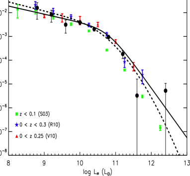
Figure 11: The local ($0<z<0.2$) TIR LF determined using 1/$V_{\mathrm{max}}$ (filled black circles) and the parametric Bayesian method (solid and dashed black line) evaluated at $z=0.1$. The filled green squares are obtained from Sanders et al. (2003) (S03), the filled blue stars are from Rodighiero et al. (2010) (R10) and the filled red triangles are from Vaccari et al. (2010) (V10).

In Figure 10, we compare our TIR LF with literature values in the higher redshift bins. As shown in this figure, our TIR LF shown is broadly consistent with the published results in the redshift bins $[0.2-0.4]$ and $[0.4-0.8]$. We find excellent agreement when we compare our 1/$V_{\mathrm{max}}$ LF in the redshift bins $[0.3-0.45]$ and $[0.6-0.8]$ to the values of Le Floc’h et al. (2005) and Rodighiero et al. (2010) in the same redshift bins. In the highest redshift bin considered here, our 1/$V_{\mathrm{max}}$ and the parametric LF show poor agreement because we are limited by the number of objects in these redshift bins. However when we compare the LFs with the values from Caputi et al. (2007), and Le Floc’h et al. (2005), we find good agreement between the parametric LF and the literature values. Comparing our LF with the Magnelli et al. (2009) and Rodighiero et al. (2010) LF values (orange filled upside down triangles) shows a slight difference in that the binned estimates are lower than our parametric and 1/$V_{\mathrm{max}}$ LF. Magnelli et al. (2009) investigated the difference between their and the Le Floc’h et al. (2005) LF values and found that the difference appears to be because of the choice of SED library and the correlation used to convert $\nu$L_ν to L_IR. Thus, this may also be the reason for the difference seen in the comparison of our work with theirs. Therefore although our 1/$V_{\mathrm{max}}$ LF values in the highest redshift bins are less robust, our parametric TIR LF and its evolution conforms to results that have been determined previously.

	$\log\Phi$ (Mpc-3)
$\log\mathrm{L_{IR}}$ (L${}_{\odot})$	$0<{z}\leq 0.2$	$0.2<{z}\leq 0.4$	$0.4<{z}\leq 0.8$	$0.8<{z}\leq 1.2$
8.8	$-1.80^{+0.22}_{-0.49}$
9.2	$-2.08^{+0.18}_{-0.32}$
9.6	$-2.51^{+0.19}_{-0.36}$
10.0	$-2.42^{+0.08}_{-0.10}$
10.4	$-2.69^{+0.07}_{-0.09}$	$-2.96^{+0.24}_{-0.64}$
10.8	$-3.02^{+0.07}_{-0.09}$	$-2.73^{+0.11}_{-0.15}$
11.2	$-3.74^{+0.13}_{-0.19}$	$-3.09^{+0.06}_{-0.06}$	$-3.60^{+0.13}_{-0.19}$
11.6	$-5.49^{+0.69}_{-5.49}$	$-3.86^{+0.08}_{-0.10}$	$-3.43^{+0.14}_{-0.21}$
12.0	–	$-4.74^{+0.17}_{-0.30}$	$-3.96^{+0.08}_{-0.09}$	$-4.53^{+0.24}_{-0.56}$
12.4	$-5.28^{+0.31}_{-5.28}$		$-4.95^{+0.13}_{-0.18}$	–
12.8			$-5.56^{+0.20}_{-0.38}$	$-4.57^{+0.27}_{-0.88}$
13.2				$-5.42^{+0.90}_{-5.42}$

Table 5: The 1/$V_{\mathrm{max}}$ TIR LF values.

6 Discussion

6.1 Evolution of the Infrared Luminosity Density

Having determined the global evolution of the TIR LF in the redshift range $0<z<1.2$, we can now estimate how the comoving IR luminosity density (IRLD) and the space density of LIRGs and ULIRGs evolves with redshift. This is important because it allows us to evaluate the relative importance of IR luminous galaxies and their contribution to the CSFRD (associated with obscured star formation) out to $z\sim 1.2$.

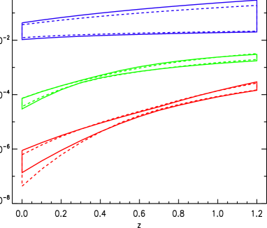
Figure 12: Evolution of the space density of normal galaxies (solid and dashed blue region), LIRGs (solid and dashed green region) and ULIRGs (solid and dashed red region) up to $z=1.2$. The solid and dashed line regions includes 68% of the posterior probability for the double power-law and power-law and log-normal LF models respectively.

We show in Figure 12, the space density of normal galaxies (blue regions), LIRGs (green region) and ULIRGs (red region), which shows rapid evolution in the number density of LIRGs and ULIRGs while the number density of normal galaxies remains constant. The number density of LIRGs increases by a factor of $\sim 43^{+11}_{-12}$ for the double power-law LF model and $\sim 37^{+18}_{-06}$ for the power-law and log-normal LF model between $z=0$ and $z=1$, which is in agreement with the estimate of Magnelli et al. (2009), who find a factor of 40.

Magnelli et al. (2009) estimate an increase in the number density of ULIRGs by a factor of $\sim 100$ at $z\sim 1$ than in the local Universe, while in Figure 12 ULIRGs increase by a factor of $\sim 316^{+246}_{-138}$ for model 1 and for model 2 the factor is $\sim 870^{+479}_{-499}$. The difference between the values of model 1 and 2 is because of the steeper drop-off at the bright end of the LF for the power-law and log-normal LF model. Nonetheless, the 68% credible intervals shown in Figure 12 for the two LF models are almost identical except for the ULIRG population, where the error for the power-law and log-normal LF model is larger.

We model the evolution of the space density of ULIRGs as $\propto(1+z)^{n}$, with $n=8.30^{+0.83}_{-0.83}$, which is consistent with the results of Kim & Sanders (1998) who find $n=7.6\pm 3.2$. Goto et al. (2011) use FIR data from AKARI to find that ULIRGs evolve with $n=10.0\pm 0.5$, which is similar to the value determined in our study. In contrast, Jacobs et al. (2011) have estimated $n\simeq 6\pm 1$ using a sample of 160 µm selected sources from Spitzer observations of the 1 deg² ISO Deep Field region in the LH. Their analysis however is based on only 40 galaxies while the current study includes 634 sources and therefore the value determined here should be more accurate and reliable.

In Figure 13 we show the IRLD which is calculated by $\Omega_{\mathrm{IR}}$ = $\int{L}\Phi(L,z|\{\theta\})\thinspace{dL}$. We only display IRLD determined using the double power-law LF model because the 68% credible interval is almost identical when IRLD is calculated using the power-law and log-normal LF model. We follow the method presented in Le Floc’h et al. (2005) by determining IRLD for IR luminous galaxies (LIRGs and ULIRGs) and “normal” galaxies as a function of redshift. The evolution of $\Omega_{\mathrm{IR}}$ is also represented in terms of an IR equivalent SFR using the calibration given by Equation 16. The figure shows that our results are in agreement with what has been predicted from previous studies, particularly with the results of Rodighiero et al. (2010). At the present epoch, most ($\sim 85^{+03}_{-13}\%$) of the star formation activity is taking place in normal galaxies which have low extinction. As we move to higher redshifts, LIRGs evolve rapidly and dominate the star formation activity beyond $z\sim 0.55^{+0.10}_{-0.05}$.

The model also suggests that, LIRGs and ULIRGs are responsible for $\sim 68^{+10}_{-07}$ per cent of the total IRLD at $z=1.2$. At $z=0$, LIRGs and ULIRGs are responsible for less than $10^{+08}_{-02}\%$ of the IRLD, while at $z=1$, they produce $\sim 66^{+10}_{-05}\%$ of it. These values are consistent with estimates of Le Floc’h et al. (2005) while Magnelli et al. (2009) suggest that LIRGs and ULIRGs produce less than 2% of the IRLD. This difference is most likely due to the fact that Magnelli et al. (2009) use the faint-end power-law index, $\alpha=-0.6$, from the IRAS TIR LF of Sanders et al. (2003), which is steeper than the value used in this study ($\alpha=0.34^{+0.10}_{-0.12}$ for the double power-law LF model) and this would lead to a higher contribution of normal galaxies to the IRLD at $z=0$.

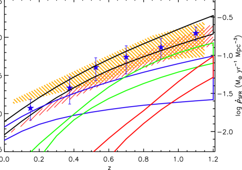
Figure 13: Evolution of the IRLD up to $z=1.2$ (solid black line region) and the contribution by normal galaxies (solid blue line region), LIRGs (solid green line region) and ULIRGs (solid red line region) determined using the double power-law LF model. The black solid region includes 68% of the posterior probability. The red line region is taken from Le Floc’h et al. (2005), orange line region is from Magnelli et al. (2009) and blue filled stars are taken from Rodighiero et al. (2010).

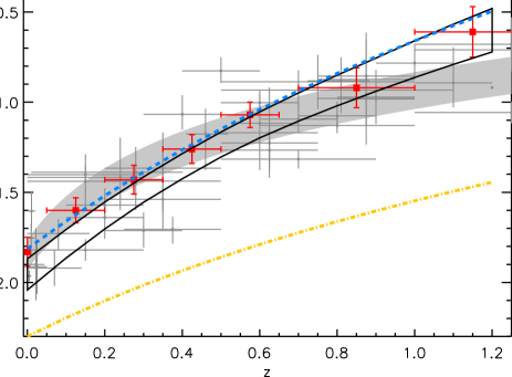
Figure 14: Evolution of the CSFRD up to $z=1.2$ (solid black line region). The solid black line region includes 68% of the posterior probability. The grey points are taken from Hopkins (2004) representing the CSFRD from various estimators. The red filled squares are CSFRD estimates from Rujopakarn et al. (2010). The orange dash-dot line is the UV dust extinction uncorrected CSFRD from Schiminovich et al. (2005) and the light blue dashed line represents the total CSFRD defined as the sum of the IR and UV dust extinction uncorrected SFR densities. The shaded grey region is the $3\sigma$ best-fitting regions CSFRD from Hopkins & Beacom (2006).

6.2 Evolution of the Cosmic Star Formation Rate Density

In Figure 14, we show the CSFRD as a function of redshift up to $z=1.2$ and compare our results with the CSFRD estimates compiled by Hopkins (2004) and Hopkins & Beacom (2006) at wavelengths ranging from the X-ray to radio. We highlight for comparison, in filled blue squares the SFR derived from 24 µm observations taken from Rujopakarn et al. (2010) (blue filled squares in Figure 14). Overall, our prediction of $\rho_{\textsc{sfr}}$ show a good agreement with the results determined from previous experiments. At $z=0$, the CSFRD is $1.04^{+0.31}_{-0.13}\times 10^{-2}$ M_⊙ yr^-1 Mpc^-3 which agrees with previous values of the local $\rho_{\textsc{sfr}}$ that have properly accounted for the internal extinction of the galaxy but slightly lower than the estimate of Rujopakarn et al. (2010) who find a local $\rho_{\textsc{sfr}}$ of $1.65\times 10^{-2}$ M_⊙ yr^-1 Mpc^-3 (assuming a Salpeter 1955 IMF). The dust unobscured CSFRD estimated by Schiminovich et al. (2005) (dot dashed orange line) is also displayed in Figure 14. At $z=0$, the dust unobscured CSFRD is estimated to be $\sim 5.01\times 10^{-3}$ M_⊙ yr^-1 Mpc^-3 and therefore without dust extinction corrections, the local CSFRD would be underestimated by $\sim 65^{+8}_{-30}$ per cent. Modelling $\rho_{\textsc{sfr}}$ as $\propto(1+z)^{Q}$, implies $Q=3.82^{+0.25}_{-0.16}$, which is higher than the value reported by Hopkins (2004) ($Q=3.29\pm 0.26$) but consistent with Rujopakarn et al. (2010) ($Q=3.50\pm 0.20$). The results presented here show that in general, most of the star formation over the last 8 billion years has taken place in dust obscured galaxies.

6.3 Future prospects

In Section 5, we have presented the results of the evolution of the far-IR luminosity functions in the SWIRE XMM-LSS and Lockman Hole fields, based on a spectroscopic redshift sample. The 70 µm and TIR LFs were constructed using the sample selected with S${}_{70}>10$ mJy and $r<22$ and the 160 µm LF was constructed using sources with S${}_{160}>60$ mJy and $r<22$. In this section we discuss the limitations of the sample selection and the methodology in constructing the FIR LFs and suggest improvements that could be carried out in order to obtain better estimates of LFs.

We chose to study the evolution of the FIR LFs using only spectroscopic redshifts in order to reduce the uncertainties related to photometric redshifts as stated in Section 1. Some previous studies of the evolution of the IR LFs that have utilised photometric redshift (Pérez-González et al., 2005; Babbedge et al., 2004; Wang & Rowan-Robinson, 2010) account for the uncertainty in the redshift by performing Monte Carlo analysis, where each source’s photometric redshift is replaced by a redshift drawn randomly from a Gaussian distribution centred on the original photometric redshift and then iterating the LF procedure. Few authors (Chen et al., 2003; Aird et al., 2010) have attempted to account for this uncertainty by modifying the likelihood function in Equation LABEL:eq:lhfunc and including the actual redshift probability distribution function for each source likelihood ($p(\{L_{i},z_{i}\}|\{\theta\})$) rather than a gaussian approximation. Therefore including sources with photometric redshifts will not only increase the sample size but we will be able to apply a fainter magnitude cut in the optical and reach higher redshifts.

At IR wavelengths, the sample includes sources up to the flux limit of the SWIRE survey but with a strict magnitude cut of $r<22$ our sample will not include those IR sources that are also optically faint. For the present sample, $>50\%$ of the 70 µm sources at 10 mJy have an optical counterpart that is brighter than 22 mag in the $r-$band and therefore inclusion of the photometric redshifts will also reduce the dependence on the spectroscopic incompleteness weights $w_{i}$. Since future large surveys will discover many millions of galaxies, photometric redshifts will play a vital role in any statistical analysis and therefore the inclusion of this in our studies will be one of the next key step.

The other limitation of the work is that in the parametric method, we have assumed a single evolving population. For the 70 µm and the TIR LF the selection functions are calculated assuming an M82 SED template and for the 160 µm LF we have used a mixture of M82 and Cirrus SED. As shown in Figure 3, we observe a gradual change in the best-fit SED type as we move out to higher redshift, with low redshift sources fit with a cirrus dominated SED and the higher redshift sources fit with a starburst dominated SED. This implies that the starburst component of the IR SED must evolve much faster than the cirrus component and therefore this evolution must be taken into account when studying the evolution of LFs using parametric methods. Therefore studying the evolution of each SED component will be the second step in studying the evolution of the FIR LFs.

7 Summary and Conclusion

We have presented a new observational determination of the FIR LFs using 70 µm selected sources from the SWIRE survey with spectroscopic redshifts. The primary sample was selected from the photometric redshift catalogueue of Rowan-Robinson et al. (2008), which contains over 1 million IR sources estimated by combining optical and IRAC 3.6 and 4.5 µm photometry. We computed the rest-frame 70 µm and TIR LF using sources with $S_{70}>10$mJy and $r<22$ and studied their evolution out to $z=1.2$. The evolution of the 160 µm LF was determined using $S_{160}>60$mJy and $r<22$ out to $z=0.5$.

We use the multiwavelength optical to IR data to model the SED for each source in our sample to estimate the rest-frame monochromatic luminosities to determine the 70 and 160 µm LFs using Bayesian parametric and the 1/$V_{\mathrm{max}}$ methods. The work presented here is an improvement on earlier works because we use 70 µm data rather than rely on extrapolations from 24 µm. In addition, the Bayesian method is a new approach to FIR astronomy, which can be used to further the study of IR LFs. For example we can include photometric redshift data and properly account for the individual photometric redshift uncertainty of each source to investigate the evolution of the FIR LFs. The study of the evolution of FIR LFs using photometric redshifts will be presented in a future paper. In our analysis we have corrected for the optical and IR selection biases and incompleteness of the spectroscopic sample, which have allowed us to accurately construct the LFs.

The parametric Bayesian FIR LFs were determined using two LF models; a double power-law and a power-law and log-normal models. Comparison of the two models with the binned 1/$V_{\mathrm{max}}$ estimates showed that both LF models provide a good fit to the 70 µm and TIR LFs. For the 160 µm LF however, the power-law and log-normal LF was found to underestimate the number density of sources at L₁₆₀ $>10^{11}$ L_⊙ when compared to the binned LF estimates, implying that the double power-law LF model provides a better description of FIR LFs.

The evolution of FIR LFs was modelled using a pure luminosity evolution model. The rest-frame 70 µm LF was found to evolve rapidly in luminosity with $\alpha_{\textsc{l}}$ $=3.39^{+0.12}_{-0.22}$ for model 1 and $\alpha_{\textsc{l}}$ $=3.41^{+0.18}_{-0.25}$ for model 2. Thus the choice of LF model does not have a large effect on the evolution of the 70 µm LF. The 160 µm LF was found to evolve with $\alpha_{\textsc{l}}$ $=5.73^{+0.29}_{-0.45}$ for model 1 and $\alpha_{\textsc{l}}$ $=5.62^{+0.21}_{-0.45}$ for model 2. The faster rate of evolution of the 160 µm LF is consistent with the study of Takeuchi et al. (2006) which finds the ISO 170 µm LF evolves with $\alpha_{\textsc{l}}$ $=5.0^{+2.3}_{-0.5}$. Since cooler galaxies are detected more effectively at 160 µm than at shorter wavelengths, the strong evolution implies the presence of large amounts of cool dust at higher redshifts.

Finally, we used the best-fit SEDs to estimate total IR luminosities of each source to derive the TIR LF to $z=1.2$. The SWIRE TIR LF showed good agreement when compared with literature values estimated from Spitzer and Herschel data across all redshifts bins. The TIR LF evolves with $\text{\hbox{$\alpha_{\textsc{l}}$}}=3.82^{+0.23}_{-0.20}$ for model 1 and $\text{\hbox{$\alpha_{\textsc{l}}$}}=3.82^{+0.25}_{-0.16}$ for model 2 corroborating the conclusions of previous results from Spitzer 24 µm studies which find strong luminosity evolution. The TIR LF was then integrated to calculate the IRLD out to $z=1.2$, which confirms the rapid evolution in number density of LIRGs which contribute $\sim 66^{+10}_{-5}$ per cent to the IRLD, and hence the CSFRD at $z=1$. The results presented in this chapter, based on 70 µm data confirm that the bulk of the star formation at $z=1$ takes place in dust obscured objects.

8 Acknowledgements

HP acknowledges financial support from STFC. This work is based on observations made with the Spitzer Space Telescope, which is operated for NASA by the Jet Propulsion Laboratory, California Institute of Technology.

References

- Aird et al. (2008) Aird J., Nandra K., Georgakakis A., Laird E. S., Steidel C. C., Sharon C., 2008, MNRAS, 387, 883
- Aird et al. (2010) Aird J., Nandra K., Laird E. S., et al., 2010, MNRAS, 401, 2531
- Appleton et al. (2004) Appleton P. N., Fadda D. T., Marleau F. R., et al., 2004, ApJS, 154, 147
- Avni & Bahcall (1980) Avni Y., Bahcall J. N., 1980, ApJ, 235, 694
- Babbedge et al. (2006) Babbedge T. S. R., , Rowan-Robinson M., Vaccari M., et al., 2006, MNRAS, 370, 1159
- Babbedge et al. (2004) Babbedge T. S. R., Rowan-Robinson M., Gonzalez-Solares E., et al., 2004, MNRAS, 353, 654
- Bavouzet et al. (2008) Bavouzet N., Dole H., Le Floc’h E., et al., 2008, A&A, 479, 83
- Berta et al. (2007) Berta S., Lonsdale C. J., Siana B., et al., 2007, A&A, 467, 565
- Bertin & Arnouts (1996) Bertin E., Arnouts S., 1996, A&AS, 117, 393
- Béthermin et al. (2010a) Béthermin M., Dole H., Beelen A., Aussel H., 2010a, A&A, 512, A78+
- Béthermin et al. (2010b) Béthermin M., Dole H., Cousin M., Bavouzet N., 2010b, A&A, 516, A43+
- Caputi et al. (2007) Caputi K. I., Lagache G., Yan L., et al., 2007, ApJ, 660, 97
- Chary & Elbaz (2001) Chary R., Elbaz D., 2001, ApJ, 556, 562
- Chen et al. (2003) Chen H.-W., Marzke R. O., McCarthy P. J., et al., 2003, ApJ, 586, 745
- Christlein et al. (2009) Christlein D., Gawiser E., Marchesini D., Padilla N., 2009, MNRAS, 400, 429
- Clements et al. (2001) Clements D. L., Desert F., Franceschini A., 2001, MNRAS, 325, 665
- Dale & Helou (2002) Dale D. A., Helou G., 2002, ApJ, 576, 159
- Dunne et al. (2011) Dunne L., Gomez H. L., da Cunha E., et al., 2011, MNRAS, 417, 1510
- Dye et al. (2010) Dye S., Dunne L., Eales S., et al., 2010, A&A, 518, L10
- Elbaz et al. (2002) Elbaz D., Cesarsky C. J., Chanial P., et al., 2002, A&A, 384, 848
- Fixsen et al. (1998) Fixsen D. J., Dwek E., Mather J. C., Bennett C. L., Shafer R. A., 1998, ApJ, 508, 123
- Furusawa et al. (2008) Furusawa H., Kosugi G., Akiyama M., et al., 2008, ApJS, 176, 1
- Gelman et al. (2004) Gelman A., Carlin J., Stern H., Rubin D., 2004, Bayesian Data Analysis, 2nd edn. New York: Chapman and Hall
- Goto et al. (2011) Goto T., Arnouts S., Malkan M., et al., 2011, MNRAS, 414, 1903
- Goto et al. (2010) Goto T., Takagi T., Matsuhara H., et al., 2010, A&A, 514, A6+
- Hastings (1970) Hastings W. K., 1970, Biometrika, 57, 97
- Hogg (1999) Hogg D. W., 1999, ArXiv Astrophysics e-prints
- Hopkins (2004) Hopkins A. M., 2004, ApJ, 615, 209
- Hopkins & Beacom (2006) Hopkins A. M., Beacom J. F., 2006, ApJ, 651, 142
- Hoyle et al. (2005) Hoyle F., Rojas R. R., Vogeley M. S., Brinkmann J., 2005, ApJ, 620, 618
- Ilbert et al. (2005) Ilbert O., Tresse L., Zucca E., et al., 2005, A&A, 439, 863
- Irwin & Lewis (2001) Irwin M., Lewis J., 2001, NewAR, 45, 105
- Jacobs et al. (2011) Jacobs B. A., Sanders D. B., Rupke D. S. N., et al., 2011, AJ, 141, 110
- Kelly et al. (2008) Kelly B. C., Fan X., Vestergaard M., 2008, ApJ, 682, 874
- Kennicutt (1998) Kennicutt Jr. R. C., 1998, ARA&A, 36, 189
- Kim & Sanders (1998) Kim D.-C., Sanders D. B., 1998, ApJS, 119, 41
- Lagache et al. (2003) Lagache G., Dole H., Puget J.-L., 2003, MNRAS, 338, 555
- Le Fèvre et al. (2004) Le Fèvre O., Mellier Y., McCracken H. J., et al., 2004, A&A, 417, 839
- Le Floc’h et al. (2005) Le Floc’h E., Papovich C., Dole H., et al., 2005, ApJ, 632, 169
- Lonsdale et al. (2004) Lonsdale C., Polletta M. d. C., Surace J., et al., 2004, ApJS, 154, 54
- Lonsdale et al. (2003) Lonsdale C. J., Smith H. E., Rowan-Robinson M., et al., 2003, PASP, 115, 897
- Magnelli et al. (2009) Magnelli B., Elbaz D., Chary R. R., et al., 2009, A&A, 496, 57
- Marshall et al. (1983) Marshall H. L., Tananbaum H., Avni Y., Zamorani G., 1983, ApJ, 269, 35
- Metropolis et al. (1953) Metropolis N., Rosenbluth A. W., Rosenbluth M. N., Teller A. H., Teller E., 1953, J. Chem. Phys., 21, 1087
- Pacaud et al. (2007) Pacaud F., Pierre M., Adami C., Altieri B., et al., 2007, MNRAS, 382, 1289
- Patel et al. (2011) Patel H., Clements D. L., Rowan-Robinson M., Vaccari M., 2011, MNRAS, 415, 1738
- Pérez-González et al. (2005) Pérez-González P. G., Rieke G. H., Egami E., et al., 2005, ApJ, 630, 82
- Pierre et al. (2007) Pierre M., Chiappetti L., Pacaud F., et al., 2007, MNRAS, 382, 279
- Pozzi et al. (2004) Pozzi F., Gruppioni C., Oliver S., et al., 2004, ApJ, 609, 122
- Ptak et al. (2007) Ptak A., Mobasher B., Hornschemeier A., Bauer F., Norman C., 2007, ApJ, 667, 826
- Puget et al. (1996) Puget J., Abergel A., Bernard J., et al., 1996, A&A, 308, L5+
- Rieke & Low (1972) Rieke G. H., Low F. J., 1972, ApJL, 176, L95+
- Rodighiero et al. (2010) Rodighiero G., Vaccari M., Franceschini A., et al., 2010, A&A, 515, A8+
- Rowan-Robinson et al. (2008) Rowan-Robinson M., Babbedge T., Oliver S., et al., 2008, MNRAS, 386, 697
- Rowan-Robinson et al. (2005) Rowan-Robinson M., Babbedge T., Surace J., et al., 2005, AJ, 129, 1183
- Rowan-Robinson & Crawford (1989) Rowan-Robinson M., Crawford J., 1989, MNRAS, 238, 523
- Rowan-Robinson et al. (2004) Rowan-Robinson M., Lari C., Perez-Fournon I., et al., 2004, MNRAS, 351, 1290
- Rujopakarn et al. (2010) Rujopakarn W., Eisenstein D. J., Rieke G. H., et al., 2010, ApJ, 718, 1171
- Salpeter (1955) Salpeter E. E., 1955, ApJ, 121, 161
- Sandage et al. (1979) Sandage A., Tammann G. A., Yahil A., 1979, ApJ, 232, 352
- Sanders et al. (2003) Sanders D. B., Mazzarella J. M., Kim D.-C., Surace J. A., Soifer B. T., 2003, AJ, 126, 1607
- Sanders & Mirabel (1996) Sanders D. B., Mirabel I. F., 1996, ARA&A, 34, 749
- Saunders et al. (1990) Saunders W., Rowan-Robinson M., Lawrence A., et al., 1990, MNRAS, 242, 318
- Schechter (1976) Schechter P., 1976, ApJ, 203, 297
- Schiminovich et al. (2005) Schiminovich D., Ilbert O., Arnouts S., et al., 2005, ApJL, 619, L47
- Schmidt (1968) Schmidt M., 1968, ApJ, 151, 393
- Serjeant et al. (2004) Serjeant S., Carramiñana A., Gonzáles-Solares E., et al., 2004, MNRAS, 355, 813
- Soifer & Neugebauer (1991) Soifer B. T., Neugebauer G., 1991, AJ, 101, 354
- Soifer et al. (1987) Soifer B. T., Sanders D. B., Madore B. F., Neugebauer G., Danielson G. E., Elias J. H., Lonsdale C. J., Rice W. L., 1987, ApJ, 320, 238
- Surace et al. (2005) Surace J. A., Shupe D. L., Fang F., SWIRE Team, 2005, AAS, 37, 1246
- Symeonidis et al. (2011) Symeonidis M., Page M. J., Seymour N., 2011, MNRAS, 411, 983
- Symeonidis et al. (2009) Symeonidis M., Page M. J., Seymour N., et al., 2009, MNRAS, 397, 1728
- Symeonidis et al. (2010) Symeonidis M., Rosario D., Georgakakis A., et al., 2010, MNRAS, 403, 1474
- Symeonidis et al. (2008) Symeonidis M., Willner S. P., Rigopoulou D., et al., 2008, MNRAS, 385, 1015
- Takeuchi et al. (2006) Takeuchi T. T., Ishii T. T., Dole H., Dennefeld M., Lagache G., Puget J., 2006, A&A, 448, 525
- Takeuchi et al. (2003) Takeuchi T. T., Yoshikawa K., Ishii T. T., 2003, ApJL, 587, L89
- Trenti & Stiavelli (2008) Trenti M., Stiavelli M., 2008, ApJ, 676, 767
- Trichas et al. (2009) Trichas M., Georgakakis A., Rowan-Robinson M., et al.., 2009, MNRAS, 399, 663
- Vaccari et al. (2010) Vaccari M., Marchetti L., Franceschini A., et al., 2010, A&A, 518, L20+
- Wang & Rowan-Robinson (2010) Wang L., Rowan-Robinson M., 2010, MNRAS, 401, 35
- Werner et al. (2004) Werner M. W., Roellig T. L., Low F. J., et al., 2004, ApJS, 154, 1
- Zucca et al. (1994) Zucca E., Pozzetti L., Zamorani G., 1994, MNRAS, 269, 953