Averaging Fluctuations in Resolvents of Random Band Matrices

Abstract

We consider a general class of random matrices whose entries are centred random variables, independent up to a symmetry constraint. We establish precise high-probability bounds on the averages of arbitrary monomials in the resolvent matrix entries. Our results generalize the previous results of EYY2 ; EYY3 ; EKYY1 which constituted a key step in the proof of the local semicircle law with optimal error bound in mean-field random matrix models. Our bounds apply to random band matrices, and improve previous estimates from order 2 to order 4 in the cases relevant for applications. In particular, they lead to a proof of the diffusion approximation for the magnitude of the resolvent of random band matrices. This, in turn, implies new delocalization bounds on the eigenvectors. The applications are presented in a separate paper EKYY3 .

AMS Subject Classification: 15B52, 82B44, 82C44

Keywords: random band matrix, delocalization, sums of correlated random variables.

1 Introduction

Let $H=(h_{ij})$ be a complex Hermitian or real symmetric $N\times N$ random matrix with centred matrix entries that are independent up to the symmetry constraint. We assume that the variances $s_{ij}\mathrel{\vbox{\hbox{.}\hbox{.}}}=\mathbb{E}|h_{ij}|^{2}$ are normalized so that $\sum_{j}s_{ij}=1$ for each $i$, and let $\lVert s\rVert_{\infty}\mathrel{\vbox{\hbox{.}\hbox{.}}}=\max_{ij}s_{ij}$ denote the maximal variance. Let $G_{ab}(z)\mathrel{\vbox{\hbox{.}\hbox{.}}}=(H-z)^{-1}_{ab}$ denote the resolvent matrix entries evaluated at a spectral parameter $z=E+i\eta$ whose imaginary part $\eta$ is positive and small. It was established in EYY1 ; EKYY4 that

$$\Lambda\;\mathrel{\vbox{\hbox{.}\hbox{.}}}=\;\max_{a\neq b}|G_{ab}|\;\lesssim\;\sqrt{\frac{\lVert s\rVert_{\infty}}{\eta}}$$ (1.1)

with high probability for large $N$, up to factors of $N^{\varepsilon}$.

The matrix entries $G_{ab}\equiv G_{ab}(z)$ depend strongly on the entries of the $a$-th and $b$-th columns of $H$, but weakly on the other columns. Focusing on the dependence on $a$ only, this can be seen from the simple expansion formula

$$G_{ab}\;=\;-G_{aa}\sum_{i\neq a}h_{ai}G_{ib}^{(a)}\,,$$ (1.2)

where $G^{(a)}$ denotes the resolvent of the $(N-1)\times(N-1)$ minor of $H$ obtained by removing the $a$-th row and column (see Lemma 3.7 below for the general statement). Since $G^{(a)}$ is independent of the family $(h_{ai})_{i=1}^{N}$, the formula (1.2) expresses $G_{ab}$ as a sum of independent centred random variables (neglecting the prefactor $G_{aa}$ which still depends on $(h_{ai})_{i=1}^{N}$). Therefore the size of $G_{ab}$ is governed by a fluctuation averaging mechanism, similar to the central limit theorem. This is the main reason why the bound (1.1) is substantially better than the naive estimate $|G_{ab}|\leqslant\eta^{-1}$.

In this paper we investigate a more subtle phenomenon. To take a simple example, we are interested in averages of resolvent matrix entries of the form

$$\frac{1}{N}\sum_{a}G_{ab}$$ (1.3)

or, more generally, its weighted version

$$\sum_{a}s_{\mu a}G_{ab}\,,$$ (1.4)

where $\mu$ and $b$ are fixed. We aim to show that, with high probability, these averages are of order $\Lambda^{2}$ – much smaller than the naive bound $\Lambda$ which results from an application of (1.1) to each summand (we shall always work in the regime where $\Lambda\ll 1$). The mechanism behind this improved bound is that for $a\neq a^{\prime}$ the matrix entries $G_{ab}$ and $G_{a^{\prime}b}$ are only weakly correlated. To see this, note that, since $h_{ai}$ in (1.2) and $h_{a^{\prime}i}$ in the analogous formula

$$G_{a^{\prime}b}\;=\;-G_{a^{\prime}a^{\prime}}\sum_{i^{\prime}\neq a^{\prime}}h_{a^{\prime}i^{\prime}}G_{i^{\prime}b}^{(a^{\prime})}\,,$$

are independent, the correlation between $G_{ab}$ and $G_{a^{\prime}b}$ primarily comes from correlations between $h_{ai}$ and $G_{i^{\prime}b}^{(a^{\prime})}$ and between $h_{a^{\prime}i^{\prime}}$ and $G_{ib}^{(a)}$. (As above, here we neglect the less important prefactors $G_{aa}$ and $G_{a^{\prime}a^{\prime}}$.) Now $G_{i^{\prime}b}^{(a^{\prime})}$ depends only weakly on $h_{ai}$ unless some lower indices coincide: $i=i^{\prime}$ or $i=b$ or $i^{\prime}=a$. Such coincidences are atypical, however, and consequently give rise to lower-order terms. Once the smallness of the correlation between $G_{ab}$ and $G_{a^{\prime}b}$ is established, the variance of the averages (1.3) or (1.4) can be estimated. The smallness of the higher-order correlations between different resolvent matrix entries allows one to compute high moments and turn the variance bound into a high-probability bound. However, keeping track of all weak correlations among a large product of expressions of the form (1.3) with different $a$’s is rather involved, and we shall need to develop a graphical representation to do this effectively.

This idea of exploiting the weak dependence among different resolvent entries of random matrices first appeared in EYY2 and was subsequently used in EYY3 ; EKYY1 ; PY . Such estimates provide optimal error bounds in the local semicircle law – a basic ingredient in establishing the universality of local statistics of for Wigner matrices.

Our main result in this paper estimates with high probability (weighted) averages of general monomials in the resolvent matrix entries and their complex conjugates, where the averaging is performed on a subset of the indices. A more complicated example is

$$\sum_{a,b}s_{\mu a}s_{\nu b}\Bigl{(}{|G_{ab}|^{2}|G_{a\rho}|^{2}-\mathbb{E}_{ab}|G_{ab}|^{2}|G_{a\rho}|^{2}}\Bigr{)}\,,$$ (1.5)

where $\mu$, $\nu$, and $\rho$ are fixed. Here we subtract from each summand its partial expectation $\mathbb{E}_{ab}$ with respect to the random variables in the $a$-th and $b$-th columns of $H$. (Note that we could also have subtracted $\mathbb{E}_{a}G_{ab}$ in (1.3) and (1.4) as well, but this expectation turns out to be negligible, unlike the expectations of the manifestly positive quantity $|G_{ab}|^{2}|G_{a\rho}|^{2}$ in (1.5)).

The expression (1.5) can trivially be estimated by $\Lambda^{4}$ with high probability using the estimate (1.1) on each summand (neglecting that diagonal resolvent matrix entries $G_{aa}$ require a different estimate). However, we can in fact do better: the averaging over two indices gives rise to a cancellation of fluctuations, due to the weak correlations among the summands. Since each averaging independently yields an extra factor $\Lambda$ as in (1.3) and (1.4), it seems plausible that the naive estimate of order $\Lambda^{4}$ on (1.5) can be improved to $\Lambda^{6}$. This in fact turns out to be correct in the example (1.5), but in general the principle that each averaging yields one extra $\Lambda$ factor is not optimal. Depending on the structure of the monomial, the gain may be more than a single factor $\Lambda$ per averaged index. For example, averaging in the index $a$ in the quantities

$$\text{(I)}\;\mathrel{\vbox{\hbox{.}\hbox{.}}}=\;\sum_{a}s_{\mu a}\bigl{(}{G_{ba}G_{ab}^{*}-\mathbb{E}_{a}G_{ba}G_{ab}^{*}}\bigr{)}\qquad\text{and}\qquad\text{(II)}\;\mathrel{\vbox{\hbox{.}\hbox{.}}}=\;\sum_{a}s_{\mu a}\bigl{(}{G_{ba}G_{ab}-\mathbb{E}_{a}G_{ba}G_{ab}}\bigr{)}$$ (1.6)

has different effects. The naive estimate using (1.1) yields $\Lambda^{2}$ for both quantities, but (I) is in fact of order $\Lambda^{4}$ while the (II) is only of order $\Lambda^{3}$ (all estimates are understood with high probability).

The reason behind the gain of a factor $\Lambda^{2}$ over the naive size in case of (I) is quite subtle. We already mentioned that the dependence of $G_{ab}$ on the random variables in the $c$-th column is weak if $c\neq a,b$. This is manifested in the identity

$$G_{ab}\;=\;G_{ab}^{(c)}+\frac{G_{ac}G_{cb}}{G_{cc}}\,.$$ (1.7)

(This identity first appeared in EYY1 ; see Lemma 3.7 below for a precise statement and related formulas.) Since $G_{ab}^{(c)}$ is independent of the $c$-th column, the $c$-dependence of $G_{ab}$ is contained in the second term of (1.7). This term is naively of order $\Lambda^{2}$, i.e. smaller than the main term (accepting that $G_{cc}$ in the denominator is harmless; in fact it turns out to be bounded from above and below by universal positive constants). Computing the variance of (I) results in a double sum $\sum_{a}\sum_{c}$. We shall see that, since the first term of (1.7) is independent of $c$, the leading order contribution to the variance in fact comes from the second term. This yields an improvement of one $\Lambda$ over the naive bound $\Lambda^{2}$. These ideas lead to a bound of order $\Lambda^{3}$ for both (I) and (II). The idea of using averaging to improve a trivial bound on resolvent entries by an extra factor $\Lambda$ was central in EYY2 . In that paper this idea was applied to a specific quantity analogous to

$$\frac{1}{N}\sum_{a}(1-\mathbb{E}_{a})\frac{1}{G_{aa}}\,.$$ (1.8)

When we compute a high moment of the quantities in (1.6), we successively use formulas (1.7) and (1.2) and take partial expectation in the expanded indices. The result is the average of a high-order monomial of resolvent matrix entries. Whether this averaging reduces the naive size depends on the precise structure of the monomial. For example,

$$\sum_{c}s_{\mu c}G_{bc}G_{cb}^{*}\;=\;\sum_{c}s_{\mu c}|G_{bc}|^{2}=O(\Lambda^{2})$$ (1.9)

and this estimate is optimal, while

$$\sum_{c}s_{\mu c}G_{bc}G_{cb}\;=\;O(\Lambda^{3}).$$ (1.10)

It turns out that average of the high-order monomial obtained from computing a high moment of (I) in (1.6) contains several summations of the type (1.10), while the analogous formula for (II) contains only summations of the type (1.9) (at least to leading order). Whether the additional gain is present or not depends on the precise structure of the original monomial, in particular on how many times the averaging index appears in an entry of $G$ or $G^{*}$. In this regard the expressions (I) and (II) differ, which is the reason why their sizes differ. Our main result (Theorem 4.8) expresses the precise relation between the maximal gain and the structure of the monomial. As it turns out, this dependence is quite subtle. The main purpose of this paper is to give a systematic rule, applicable to arbitrary monomials in the resolvent entries, which determines the gain from all indices over which an average is taken. In particular, averaging over certain indices yields an improvement of order $\Lambda^{2}$; this is a novel phenomenon. This observation is crucial in the application of our results to the problem of quantum diffusion in random band matrices EKYY3 .

Finally, we shortly explain the improvement from the naive size $\Lambda^{2}$ to $\Lambda^{3}$ for the left-hand side of (1.10). It follows from the estimate of order $\Lambda^{3}$ on (II) in (1.6) and from the fact that $\mathbb{E}_{c}G_{ac}G_{cb}=O(\Lambda^{3})$ for any $a,b$. That the expectation $\mathbb{E}_{c}G_{ac}G_{cb}$ itself is smaller than its naive size $\Lambda^{2}$ may be seen by expanding $G_{ac}G_{cb}$ in the index $c$ using formulas of the type (1.2). It turns out that $\mathbb{E}_{c}G_{ac}G_{cb}$, viewed as a vector indexed by $c$ and keeping $a$ and $b$ fixed, satisfies a stable self-consistent vector equation (see (7.16)). The analysis of this equation leads to the improved bound on $\mathbb{E}_{c}G_{ac}G_{cb}$ of order $\Lambda^{3}$.

Bounds on averages of resolvents of random matrices have played an essential role in establishing the local semicircle law with an optimal error bound. We recall that in the simplest case of Wigner matrices, where $s_{ij}=N^{-1}$, the trace of the resolvent

$$m_{N}(z)\;\mathrel{\vbox{\hbox{.}\hbox{.}}}=\;\frac{1}{N}\operatorname{Tr}G(z)\;=\;\frac{1}{N}\sum_{a}G_{aa}(z)$$

is well approximated by the Stieltjes transform of the celebrated Wigner semicircle law

$$m(z)\;\mathrel{\vbox{\hbox{.}\hbox{.}}}=\;\frac{1}{2\pi}\int_{-2}^{2}\frac{\sqrt{4-x^{2}}}{x-z}\,\mathrm{d}x\,.$$

The optimal bound is

$$\lvert m(z)-m_{N}(z)\rvert\;\lesssim\;\frac{1}{N\eta}$$ (1.11)

with high probability (see EYY3 for the precise statement and the history of this result). One of the main steps in proving this optimal bound is to exploit that $G_{aa}$ and $G_{a^{\prime}a^{\prime}}$ are only weakly correlated for $a\neq a^{\prime}$. Hence the average of $G_{aa}$ in $a$ in the definition of $m_{N}(z)$ fluctuates on a smaller scale than the fluctuations of $G_{aa}$. Various forms of this fluctuation averaging were formulated in EYY2 ; EYY3 ; EKYY1 . They were the key inputs to prove (1.11) and its analogue for the sample covariance matrices in PY . In Proposition 6.1, we present a simple special case of our main result, Theorem 4.8. This proposition yields generalizations of estimates analogous to the previous fluctuation averaging bounds with a more streamlined proof. A somewhat different simplification was given in PY .

On the one hand, Theorem 4.8 is more general than its predecessors since it is applicable to arbitrary monomials in $G$ and $G^{*}$, and also holds for universal Wigner matrices with nonconstant variances. On the other hand, and more importantly, Theorem 4.8 gives a stronger bound because it exploits the additional cancellation effect explained in connection with the different bounds on the two quantities in (1.6). This extra cancellation mechanism was not present in EYY2 ; EYY3 ; EKYY1 ; PY .

In a separate paper EKYY3 we apply the stronger bound

$$\sum_{a}s_{\mu a}\bigl{(}{|G_{ab}|^{2}-\mathbb{E}_{a}|G_{ab}|^{2}}\bigr{)}\;=\;O(\Lambda^{4})$$ (1.12)

to derive a lower bound on the localization length of random band matrices. Extensions of the methods of EYY2 ; EYY3 ; EKYY1 ; PY would have yielded only

$$\sum_{a}s_{\mu a}\bigl{(}{|G_{ab}|^{2}-\mathbb{E}_{a}|G_{ab}|^{2}}\bigr{)}\;=\;O(\Lambda^{3})\,.$$ (1.13)

Had we had only (1.13) available in EKYY3 , the resulting estimate on the localization length would not have improved the previously known results EK1 ; EK2 on eigenvector delocalization.

We conclude this section with a roadmap of the paper. In Section 2 we define our main objects and introduce notation used throughout the paper. Our main result is Theorem 4.8 in Section 4. Before stating it in full generality, we first present a special case, Proposition 3.3, in Section 3. In order to motivate the concepts underlying Theorem 4.8, we not only state this special case but also give a sketch of its proof, in Section 3.2. This is done before the main theorem is stated. A reader who prefers an inductive presentation should follow our sections in sequential order. A reader who wants to jump quickly to the main result may skip Section 3.2. However, some concepts introduced in Section 3.2 are needed later in the proof (but not in the statement) of Theorem 4.8. The full proof of Theorem 4.8 is presented in Sections 6–9, following Section 5 where we give an outline of the proof and explain how Sections 6–9 are related.

2 Setup

Let $(h_{ij}\mathrel{\vbox{\hbox{.}\hbox{.}}}i\leqslant j)$ be a family of independent, complex-valued random variables $h_{ij}\equiv h_{ij}^{(N)}$ satisfying $\mathbb{E}h_{ij}=0$ and $h_{ii}\in\mathbb{R}$ for all $i$. For $i>j$ we define $h_{ij}\mathrel{\vbox{\hbox{.}\hbox{.}}}=\overline{h}\!\,_{ji}$, and denote by $H\equiv H_{N}=(h_{ij})_{i,j=1}^{N}$ the $N\times N$ matrix with entries $h_{ij}$. By definition, $H$ is Hermitian: $H=H^{*}$. We abbreviate

$$s_{ij}\;\mathrel{\vbox{\hbox{.}\hbox{.}}}=\;\mathbb{E}\lvert h_{ij}\rvert^{2}\,,\qquad M\;\equiv\;M_{N}\;\mathrel{\vbox{\hbox{.}\hbox{.}}}=\;\frac{1}{\max_{i,j}s_{ij}}\,.$$ (2.1)

In particular, we have the bound

$$s_{ij}\;\leqslant\;M^{-1}$$ (2.2)

for all $i$ and $j$. We introduce the $N\times N$ symmetric matrix $S\equiv S_{N}=(s_{ij})_{i,j=1}^{N}$. We assume that $S$ is (doubly) stochastic:

$$\sum_{j}s_{ij}\;=\;1$$ (2.3)

for all $i$. We shall always assume the bounds

$$N^{\delta}\;\leqslant\;M\;\leqslant\;N$$ (2.4)

for some fixed $\delta>0$.

Example 2.1 (Band matrix).

Fix $d\in\mathbb{N}$. Let $f$ be a bounded and symmetric (i.e. $f(x)=f(-x)$) probability density on $\mathbb{R}^{d}$. Let $L$ and $W$ be integers satisfying

$$L^{\delta^{\prime}}\;\leqslant\;W\;\leqslant\;L$$

for some fixed $\delta^{\prime}>0$. Define the $d$-dimensional discrete torus

$$\mathbb{T}^{d}_{L}\;=\;[-L/2,L/2)^{d}\cap\mathbb{Z}^{d}\,.$$

Thus, $\mathbb{T}^{d}_{L}$ has $N=L^{d}$ lattice points; and we may identify $\mathbb{T}_{L}^{d}$ with $\{1,\dots,N\}$. We define the canonical representative of $i\in\mathbb{Z}^{d}$ through

$$[i]_{L}\;\mathrel{\vbox{\hbox{.}\hbox{.}}}=\;(i+L\mathbb{Z}^{d})\cap\mathbb{T}^{d}_{L}\,.$$

Then $H$ is a $d$-dimensional band matrix with band width $W$ and profile function $f$ if

$$s_{ij}\;=\;\frac{1}{Z_{L}}\,f\biggl{(}{\frac{[i-j]_{L}}{W}}\biggr{)}\,.$$

It is not hard to see that $M=\bigl{(}{W^{d}+O(W^{d-1})}\bigr{)}/\lVert f\rVert_{\infty}$ as $L\to\infty$. The rows and columns of $H$ are thus indexed by the lattice points in $\mathbb{T}^{d}_{L}$, i.e. they are equipped with the geometry of $\mathbb{Z}^{d}$. For $d=1$, assuming that $f$ is compactly supported, the matrix entry $h_{ij}$ vanishes if $|i-j|$ is larger than $CW$, i.e. $H$ is a band matrix in the traditional sense.

It is often convenient to use the normalized entries

$$\zeta_{ij}\;\mathrel{\vbox{\hbox{.}\hbox{.}}}=\;(s_{ij})^{-1/2}h_{ij}\,,$$

which satisfy $\mathbb{E}\zeta_{ij}=0$ and $\mathbb{E}\lvert\zeta_{ij}\rvert^{2}=1$. (If $s_{ij}=0$ we set for convenience $\zeta_{ij}$ to be a normalized Gaussian, so that these relations remain valid. Of course in this case the law of $\zeta_{ij}$ is immaterial.) We assume that the random variables $\zeta_{ij}$ have finite moments, uniformly in $N$, $i$, and $j$, in the sense that for all $p\in\mathbb{N}$ there is a constant $\mu_{p}$ such that

$$\mathbb{E}\lvert\zeta_{ij}\rvert^{p}\;\leqslant\;\mu_{p}$$ (2.5)

for all $N$, $i$, and $j$. We make this assumption to streamline notation in the statements of results such as Theorem 4.8 and the proofs. In fact, our results hold, with the same proof, provided (2.5) is valid for some large but fixed $p$. See Remark 4.11 below for a more precise statement.

Throughout the following we use a spectral parameter $z\in\mathbb{C}$ satisfying $\operatorname{Im}z>0$. We shall use the notation

$$z\;=\;E+\mathrm{i}\eta$$

without further comment. The Stieltjes transform of Wigner’s semicircle law is defined by

$$m\;\equiv\;m(z)\;\mathrel{\vbox{\hbox{.}\hbox{.}}}=\;\frac{1}{2\pi}\int_{-2}^{2}\frac{\sqrt{4-\xi^{2}}}{\xi-z}\,\mathrm{d}\xi\,.$$ (2.6)

To avoid confusion, we remark that the Stieltjes transform $m$ was denoted by $m_{sc}$ in the papers ESY1 ; ESY2 ; ESY3 ; ESY4 ; ESY5 ; ESY6 ; ESY7 ; ESYY ; EYY1 ; EYY2 ; EYY3 ; EKYY1 ; EKYY2 , in which $m$ had a different meaning from (2.6). It is well known that the Stieltjes transform $m$ satisfies the identity

$$m(z)+\frac{1}{m(z)}+z\;=\;0\,.$$ (2.7)

We define the resolvent of $H$ through

$$G(z)\;\mathrel{\vbox{\hbox{.}\hbox{.}}}=\;(H-z)^{-1}\,,$$

and denote its entries by $G_{ij}(z)$. We also write $G^{*}(z)\mathrel{\vbox{\hbox{.}\hbox{.}}}=(G(z))^{*}=(H-\bar{z})^{-1}$. We often drop the argument $z$ and write $G\equiv G(z)$ as well as $G^{*}\equiv G^{*}(z)$.

Definition 2.2 (Minors).

For $T\subset\{1,\dots,N\}$ we define $H^{(T)}$ by

$$(H^{(T)})_{ij}\;\mathrel{\vbox{\hbox{.}\hbox{.}}}=\;\bm{\mathrm{1}}(i\notin T)\bm{\mathrm{1}}(j\notin T)h_{ij}\,.$$

Moreover, we define the resolvent of $H^{(T)}$ through

$$G^{(T)}_{ij}(z)\;\mathrel{\vbox{\hbox{.}\hbox{.}}}=\;(H^{(T)}-z)^{-1}_{ij}\,.$$

We also set

$$\sum_{i}^{(T)}\;\mathrel{\vbox{\hbox{.}\hbox{.}}}=\;\sum_{i\mathrel{\vbox{\hbox{.}\hbox{.}}}i\notin T}\,.$$

When $T=\{a\}$, we abbreviate $(\{a\})$ by $(a)$ in the above definitions; similarly, we write $(ab)$ instead of $(\{a,b\})$.

Definition 2.3 (Partial expectation and independence).

Let $X\equiv X(H)$ be a random variable. For $i\in\{1,\dots,N\}$ define the operations $P_{i}$ and $Q_{i}$ through

$$P_{i}X\;\mathrel{\vbox{\hbox{.}\hbox{.}}}=\;\mathbb{E}(X|H^{(i)})\,,\qquad Q_{i}X\;\mathrel{\vbox{\hbox{.}\hbox{.}}}=\;X-P_{i}X\,.$$

We call $P_{i}$ partial expectation in the index $i$. Moreover, we say that $X$ is independent of $T\subset\{1,\dots,N\}$ if $X=P_{i}X$ for all $i\in T$.

The following definition introduces a notion of a high-probability bound that is suited for our purposes.

Definition 2.4 (Stochastic domination).

Let $X=\bigl{(}{X^{(N)}(u)\mathrel{\vbox{\hbox{.}\hbox{.}}}N\in\mathbb{N},u\in U^{(N)}}\bigr{)}$ be a family of random variables, where $U^{(N)}$ is a possibly $N$-dependent parameter set. Let $\Psi=\bigl{(}{\Psi^{(N)}(u)\mathrel{\vbox{\hbox{.}\hbox{.}}}N\in\mathbb{N},u\in U^{(N)}}\bigr{)}$ be a deterministic family satisfying $\Psi^{(N)}(u)\geqslant 0$. We say that $X$ is stochastically dominated by $\Psi$, uniformly in $u$, if for all (small) $\varepsilon>0$ and (large) $D>0$ we have

$$\sup_{u\in U^{(N)}}\mathbb{P}\Bigl{[}{\bigl{\lvert}X^{(N)}(u)\bigr{\rvert}>N^{\varepsilon}\Psi^{(N)}(u)}\Bigr{]}\;\leqslant\;N^{-D}$$

for large enough $N\geqslant N_{0}(\varepsilon,D)$. Unless stated otherwise, throughout this paper the stochastic domination will always be uniform in all parameters apart from the parameter $\delta$ in (2.4) and the sequence of constants $\mu_{p}$ in (2.5); thus, $N_{0}(\varepsilon,D)$ also depends on $\delta$ and $\mu_{p}$. If $X$ is stochastically dominated by $\Psi$, uniformly in $u$, we use the equivalent notations

$$X\;\prec\;\Psi\qquad\text{and}\qquad X\;=\;O_{\prec}(\Psi)\,.$$

For example, using Chebyshev’s inequality and (2.5) one easily finds that

$$h_{ij}\;\prec\;(s_{ij})^{1/2}\;\prec\;M^{-1/2}\,,$$ (2.8)

so that we may also write $h_{ij}=O_{\prec}((s_{ij})^{1/2})$. The relation $\prec$ satisfies the familiar algebraic rules of order relations. For instance if $A_{1}\prec\Psi_{1}$ and $A_{2}\prec\Psi_{2}$ then $A_{1}+A_{2}\prec\Psi_{1}+\Psi_{2}$ and $A_{1}A_{2}\prec\Psi_{1}\Psi_{2}$. Moreover, if $A\prec\Psi$ and there is a constant $C>0$ such that $\Psi\geqslant N^{-C}$ and $\lvert A\rvert\leqslant N^{C}$ almost surely, then $P_{i}A\prec\Psi$ and $Q_{i}A\prec\Psi$. More general statements in this spirit are given in Lemma 3.6 below.

Let $\gamma>0$ be a fixed small positive constant and let $(\bm{\mathrm{S}}^{(N)})$ be a sequence of domains satisfying

$$\bm{\mathrm{S}}^{(N)}\;\subset\;\bigl{\{}{z\in\mathbb{C}\mathrel{\vbox{\hbox{.}\hbox{.}}}-10\leqslant E\leqslant 10\,,\;M^{-1+\gamma}\leqslant\eta\leqslant 10}\bigr{\}}\,.$$

As usual, we shall systematically omit the index $N$ on $\bm{\mathrm{S}}$.

Definition 2.5.

A positive $N$-dependent deterministic function $\Psi\equiv\Psi^{(N)}$ on $\bm{\mathrm{S}}$ is called a control parameter. The control parameter $\Psi$ is admissible if there is a constant $c>0$ such that

$$M^{-1/2}\;\leqslant\;\Psi(z)\;\leqslant\;M^{-c}$$ (2.9)

for all $N$ and $z\in\bm{\mathrm{S}}$.

In this paper we always consider families $X^{(N)}(u)=X^{(N)}_{i}(z)$ indexed by $u=(z,i)$, where $z\in\bm{\mathrm{S}}$ and $i$ takes on values in some finite (possibly $N$-dependent or empty) index set.

We slightly modify the definition (1.1) to include a control on the diagonal entries of $G$ in addition to the off-diagonal entries. For the rest of the paper, we define the ($z$-dependent) random variable

$$\Lambda(z)\;\mathrel{\vbox{\hbox{.}\hbox{.}}}=\;\max_{x,y}\bigl{\lvert}G_{xy}(z)-\delta_{xy}m(z)\bigr{\rvert}\,.$$

The variable $\Lambda$ will play the role of a random control parameter. If $\Psi$ is an admissible control parameter, the lower bound on $\Psi$ in (2.9) together with (2.8) imply that

$$h_{ij}\;\prec\;\Psi\,.$$ (2.10)

3 Simple examples and ingredients of the proof

In this section we give an informal overview of fluctuation averaging, by stating and sketching the proofs of a few simple, yet representative, cases. Our starting point will always be an admissible control parameter $\Psi$ that controls $\Lambda$, i.e. $\Lambda\prec\Psi$. In addition to $\Psi$, we introduce the secondary control parameter

$$\Phi\;\equiv\;\Phi_{\Psi}\;\mathrel{\vbox{\hbox{.}\hbox{.}}}=\;\min\bigl{\{}{\varrho\bigl{(}{\Psi+M^{-1/2}\Psi^{-1}}\bigr{)}\,,\,1}\bigr{\}}\,,$$ (3.1)

where we defined the coefficient

$$\varrho\;\mathrel{\vbox{\hbox{.}\hbox{.}}}=\;\bigl{\lVert}(1-m^{2}S)^{-1}\bigr{\rVert}_{\ell^{\infty}\to\ell^{\infty}}\,.$$ (3.2)

Thus, $\Phi$ is defined in terms of the primary control parameter $\Psi$, although we usually do not indicate this explicitly.

Remark 3.1.

We use the somewhat complicated definitions (3.1) and (3.2) because they emerge naturally from our argument, and do not require us to impose any further conditions on the matrix $H$ or the spectral parameter $z$. The parameter $\Phi$ will describe the gain associated with a charged vertex or a chain vertex; see Definitions 4.7 and 5.1 below.

In the motivating example of band matrices (Example 2.1), the parameter $\Phi$ may be considerably simplified. Indeed, in that case there is a positive constant $C$ such that

$$\varrho\;\leqslant\;\frac{C\log N}{(\operatorname{Im}m)^{2}}\,,$$ (3.3)

as proved in Proposition B.2 below. For most applications, we are interested in the bulk spectrum of the band matrix, i.e. $E\in[-2+\kappa,2-\kappa]$ for some fixed $\kappa>0$. In that case the relation $\operatorname{Im}m(z)\asymp\sqrt{\eta+2-\lvert E\rvert}$ (proved e.g. in (EYY2, , Lemma 4.2)) yields $\operatorname{Im}m\geqslant c$ for some positive constant $c$ depending on $\kappa$. We conclude that $1\leqslant\varrho\leqslant C\log N$; the logarithmic factor in the upper bound is irrelevant, since $\Phi$ will always be used as a deterministic control parameter in Definition 2.4. In summary: for the bulk spectrum of a band matrix, we may replace $\Phi$ with $\Psi+M^{-1/2}\Psi^{-1}$.

Moreover, in typical applications the imaginary part $\eta$ of the spectral parameter $z$ is small enough that $\Psi\geqslant M^{-1/4}$. In this case $\Phi$ and $\Psi$ are comparable (in the bulk spectrum), and hence interchangeable as control parameters in Definition 2.4.

Remark 3.2.

We have the lower bound

$$1/2\;\leqslant\;|1-m^{2}|^{-1}\;\leqslant\;\varrho\,,$$ (3.4)

where the first inequality follows from (3.11) below, and the second from the identity $(1-m^{2}S)^{-1}\bm{\mathrm{e}}=(1-m^{2})^{-1}\bm{\mathrm{e}}$ with the vector $\bm{\mathrm{e}}\mathrel{\vbox{\hbox{.}\hbox{.}}}=(1,\dots,1)$. We therefore have the bounds $\Psi\leqslant 2\Phi\leqslant 2$.

In this section we sketch the proof of the following result.

Proposition 3.3 (Simple examples).

Suppose that $\Lambda\prec\Psi$ for some admissible control parameter $\Psi$. Then we have

$$\frac{1}{N}\sum_{a}^{(\mu)}G_{\mu a}G_{a\mu}\;\prec\;\Psi^{2}\Phi\,,\qquad\frac{1}{N}\sum_{a}^{(\mu)}G_{\mu a}G_{a\mu}^{*}\;\prec\;\Psi^{2}$$ (3.5)

as well as

$$\frac{1}{N}\sum_{a}^{(\mu)}Q_{a}(G_{\mu a}G_{a\mu})\;\prec\;\Psi^{3}\,,\qquad\frac{1}{N}\sum_{a}^{(\mu)}Q_{a}(G_{\mu a}G_{a\mu}^{*})\;\prec\;\Psi^{3}\Phi\,.$$ (3.6)

In addition, we have the bounds

$$\frac{1}{N}\sum_{a}(G_{aa}-m)\;\prec\;\Psi\Phi\,,\qquad\frac{1}{N}\sum_{a}Q_{a}G_{aa}\;\prec\;\Psi^{2}\,.$$ (3.7)

Remark 3.4.

As explained after (3.1), typically $\Phi$ and $\Psi$ are comparable. In this case the right-hand sides of the estimates in (3.5) can be replaced with $\Psi^{3}$ and $\Psi^{2}$, those of (3.6) with $\Psi^{3}$ and $\Psi^{4}$, and those of (3.7) with $\Psi^{3}$ and $\Psi^{3}$. Thus we may keep track of the improving effect of the average using a simple power counting in the single parameter $\Psi$, replacing each $\Phi$ with a $\Psi$.

The significance of Proposition 3.3 is the following. The trivial bound $G_{a\mu}\prec\Psi$ (which follows immediately from $\Lambda\prec\Psi$) implies, for example, that $\frac{1}{N}\sum_{a}^{(\mu)}G_{\mu a}G_{a\mu}\prec\Psi^{2}$. The first estimate in (3.5) represents an improvement from $\Psi^{2}$ to $\Psi^{2}\Phi$. This improvement is due to the averaging over the index $a$ of fluctuating quantities with almost vanishing expectation. We shall refer to such vertices as charged; see Definition 4.7 below. In contrast, there is no such improvement in the second estimate of (3.5), since $G_{\mu a}G_{a\mu}^{*}=\lvert G_{\mu a}\rvert^{2}$ is always positive. If we subtract the expectation (for technical reasons, we subtract only the partial expectation, i.e. take $Q_{a}=1-P_{a}$), then the averaging becomes effective and it improves the average of $G_{\mu a}G_{a\mu}^{*}$ by two orders, from $\Psi^{2}$ to $\Psi^{3}\Phi$. Interestingly, subtracting the expectation in the average of $G_{\mu a}G_{a\mu}$ does not improve the estimate further; compare the first bounds in (3.5) and (3.6). (In fact, we get the only slightly stronger bound $\Psi^{3}$ instead of $\Psi^{2}\Phi$.) These examples indicate that the improving effect of the averaging heavily depends on the structure of the resolvent monomials.

We shall be concerned with averages of more general expressions. Roughly, we consider arbitrary monomials in the resolvent entries $(G_{ij})$. Some of the indices are summed. The summation is always performed with respect to a weight, a nonnegative quantity which sums to one. In the examples of Proposition 3.3, the weight was $N^{-1}$. Generally, we want to allow weights consisting of factors $N^{-1}$ as well as $s_{ij}$; recall that $\sum_{j}s_{ij}=\sum_{j}N^{-1}=1$. Thus, in addition to (3.5), (3.6), and (3.7) we have for example the bounds

$$\sum_{a}^{(\mu)}s_{\nu a}G_{\mu a}G_{a\mu}\;\prec\;\Psi^{2}\Phi\,,\qquad\sum_{a}^{(\mu)}s_{\nu a}Q_{a}(G_{\mu a}G_{a\mu}^{*})\;\prec\;\Psi^{3}\Phi\,,\qquad\sum_{a}s_{\nu a}(G_{aa}-m)\;\prec\;\Psi\Phi\,.$$ (3.8)

A slightly more involved average is

$$\sum_{a,b}s_{\mu a}s_{\rho b}\,Q_{b}\bigl{(}{G_{\mu a}G_{ab}G_{b\nu}^{*}G_{ab}^{*}G_{\nu a}}\bigr{)}$$ (3.9)

where $\mu$, $\nu$, and $\rho$ are fixed. In Theorem 4.8 we shall see that (3.9) is stochastically dominated by $\Psi^{6}\Phi^{2}$. This means that the double averaging and the effect of one $Q$-operation amounts to an improvement of a power three, from the trivial bound $\Psi^{5}$ to $\Psi^{6}\Phi^{2}$. It may be tempting to think that each average and each factor $Q$ improves the trivial bound by one power of $\Psi$ or $\Phi$, but this naive rule already fails in the some of the simplest examples in (3.5) and (3.6). The relation between the averaging structure and the improved power of $\Psi$ and $\Phi$ is more intricate. Our final goal (see Theorem 4.8) is to establish an optimal result for general monomials, which takes into account the precise effect of all averages.

More generally, we shall be interested in averaging arbitrary monomials $\mathcal{Z}_{\bm{\mathrm{a}}}$ in the resolvent entries. Each such monomial contains a family of summation indices $\bm{\mathrm{a}}$ and external indices $\bm{\mathrm{\mu}}$. In the example (3.9), we have

$$\mathcal{Z}_{\bm{\mathrm{a}}}\;=\;G_{\mu a}G_{ab}G_{b\nu}^{*}G_{ab}^{*}G_{\nu a}\,,\qquad\bm{\mathrm{a}}=(a,b)\,,\qquad\bm{\mathrm{\mu}}=(\mu,\nu)\,.$$ (3.10)

The most convenient way to define such a monomial $\mathcal{Z}_{\bm{\mathrm{a}}}$ is using a graph. The vertices are associated with the summation and external indices, and a resolvent entry $G_{xy}$ is represented as a directed edge from vertex $x$ to vertex $y$. We draw an edge associated with a resolvent entry $G_{xy}$ with a solid line, and an edge associated with a resolvent entry $G_{xy}^{*}$ with a dashed line. See Figure 3.1. As it turns out, the gain in powers of $\Psi$ resulting from the averaging has a simple expression in terms of such graphs. Moreover, this graphical representation is a key tool in our proofs.

Figure 3.1: Graphs associated with the monomials (from left to right) $G_{\mu a}G_{a\mu}$, $G_{\mu a}G_{a\mu}^{*}$, and $G_{\mu a}G_{ab}G_{b\nu}^{*}G_{ab}^{*}G_{\nu a}$ (from (3.10)).

Note that neither the $Q$-factors nor the averaging weights are encoded in the graphical structure. Later we shall give a more precise definition of the class of weights we consider, but as an orientation to the reader, we emphasize that they play a secondary role. As long as the weights ensure an effective averaging over at least $M$ values of each summation index, their final role is simply accounted for in the additional factor $M^{-1/2}\Psi^{-1}$ in the definition of $\Phi$. The key improvement on the power of $\Psi$ in the final estimate is solely determined by the structure of $\mathcal{Z}_{\bm{\mathrm{a}}}$ and by the locations of the $Q$-factors.

3.1.  Preliminaries

In this subsection we collect some basic facts that will be used throughout the paper. We use $C$ to denote a generic large positive constant, which may depend on some fixed parameters and whose value may change from one expression to the next. For two positive quantities $A_{N}$ and $B_{N}$ we use the notation $A_{N}\asymp B_{N}$ to mean $C^{-1}A_{N}\leqslant B_{N}\leqslant CA_{N}$.

Lemma 3.5.

There is a constant $c>0$ such that for $E\in[-10,10]$ and $\eta\in(0,10]$

$$c\;\leqslant\;\lvert m(z)\rvert\;\leqslant\;1\,.$$ (3.11)

Proof.

See Lemma 4.2 in EYY2 . ∎

The following lemma collects basic algebraic properties of stochastic domination $\prec$.

Lemma 3.6.

1. Suppose that $X(u,v)\prec\Psi(u,v)$ uniformly in $u\in U$ and $v\in V$. If $\lvert V\rvert\leqslant N^{C}$ for some constant $C$ then

   $$\sum_{v\in V}X(u,v)\;\prec\;\sum_{v\in V}\Psi(u,v)$$

   uniformly in $u$.

2. Suppose that $X_{1}(u)\prec\Psi_{1}(u)$ uniformly in $u$ and $X_{2}(u)\prec\Psi_{2}(u)$ uniformly in $u$. Then

   $$X_{1}(u)X_{2}(u)\;\prec\;\Psi_{1}(u)\Psi_{2}(u)$$

   uniformly in $u$.

3. Suppose that $\Psi(u)\geqslant N^{-C}$ for all $u$ and that for all $p$ there is a constant $C_{p}$ such that $\mathbb{E}\lvert X(u)\rvert^{p}\leqslant N^{C_{p}}$ for all $u$. Then, provided that $X(u)\prec\Psi(u)$ uniformly in $u$, we have

   $$P_{a}X(u)\;\prec\;\Psi(u)\qquad\text{and}\qquad Q_{a}X(u)\;\prec\;\Psi(u)$$

   uniformly in $u$ and $a$.

Proof.

The claims (i) and (ii) follow from a simple union bound. The claim (iii) follows from Chebyshev’s inequality, using a high-moment estimate combined with Jensen’s inequality for partial expectation. We omit the details. ∎

We shall frequently make use of Schur’s well-known complement formula, which we write as

$$\frac{1}{G_{ii}^{(T)}}\;=\;h_{ii}-z-\sum_{k,l}^{(Ti)}h_{ik}G_{kl}^{(Ti)}h_{li}\,,$$ (3.12)

where $i\notin T\subset\{1,\dots,N\}$.

The following resolvent identities form the backbone of all of our calculations. The idea behind them is that a resolvent matrix entry $G_{ij}$ depends strongly on the $i$-th and $j$-th columns of $H$, but weakly on all other columns. The first set of identities (called Family A) determines how to make a resolvent matrix entry $G_{ij}$ independent of an additional index $k\neq i,j$. The second set of identities (Family B) expresses the dependence of a resolvent matrix entry $G_{ij}$ on the matrix entries in the $i$-th or in the $j$-th column of $H$.

Lemma 3.7 (Resolvent identities).

For any Hermitian matrix $H$ and $T\subset\{1,\dots,N\}$ the following identities hold.

Family A.

For $i,j,k\notin T$ and $k\neq i,j,$ we have

$$G_{ij}^{(T)}\;=\;G_{ij}^{(Tk)}+\frac{G_{ik}^{(T)}G_{kj}^{(T)}}{G_{kk}^{(T)}}\,,\qquad\frac{1}{G_{ii}^{(T)}}\;=\;\frac{1}{G_{ii}^{(Tk)}}-\frac{G_{ik}^{(T)}G_{ki}^{(T)}}{G_{ii}^{(T)}G_{ii}^{(Tk)}G_{kk}^{(T)}}\,.$$ (3.13)

Family B.

For $i,j\notin T$ satisfying $i\neq j$ we have

$$G_{ij}^{(T)} \;=\;-G_{ii}^{(T)}\sum_{k}^{(Ti)}h_{ik}G_{kj}^{(Ti)}\;=\;-G_{jj}^{(T)}\sum_{k}^{(Tj)}G_{ik}^{(Tj)}h_{kj}$$ (3.14a)

$$G_{ij}^{(T)} \;=\;G_{ii}^{(T)}G_{jj}^{(Ti)}\biggl{(}{-h_{ij}+\sum_{k,l}^{(Tij)}h_{ik}G_{kl}^{(Tij)}h_{lj}}\biggr{)}\,,$$ (3.14b)

$$\frac{1}{G^{(T)}_{ii}} \;=\;\frac{1}{m}-\bigl{(}{-h_{ii}+Z_{i}^{(T)}+U_{i}^{(Ti)}}\bigr{)}\,,$$ (3.14c)

where we defined

$$Z_{i}^{(T)}\;\mathrel{\vbox{\hbox{.}\hbox{.}}}=\;Q_{i}\sum_{k,l}^{(Ti)}h_{ik}G_{kl}^{(Ti)}h_{li}\,,\qquad U_{i}^{(S)}\;\mathrel{\vbox{\hbox{.}\hbox{.}}}=\;\sum_{k}^{(S)}s_{ik}G_{kk}^{(S)}-m\,.$$ (3.15)

Proof.

The first identity of (3.13) was proved in Lemma 4.2 of EYY1 . The second identity of (3.13) is an immediate consequence of the first. The identities (3.14a) were proved in Lemma 6.10 of EKYY2 , and (3.14b) follows by iterating (3.14a) twice. Finally, (3.14c) (together with (3.15)) follows easily from (3.12), (2.7), the partition $1=Q_{i}+P_{i}$, and the definition (2.1). ∎

Next, we record a simple estimate on resolvent entries of minors. For $T\subset\{1,\dots,N\}$ define the random variable

$$\Lambda^{(T)}(z)\;\mathrel{\vbox{\hbox{.}\hbox{.}}}=\;\max_{i,j\notin T}\Bigl{\lvert}G_{ij}^{(T)}(z)-\delta_{ij}m(z)\Bigr{\rvert}\,.$$

Lemma 3.8 (Bound on $\Lambda^{(T)}$).

Suppose that $\Lambda\prec\Psi$ for some admissible control parameter $\Psi$. Then for any fixed $\ell\in\mathbb{N}$ we have

$$\Lambda^{(T)}\;\prec\;\Psi$$ (3.16)

provided that $\lvert T\rvert\leqslant\ell$. (The threshold $N_{0}(\varepsilon,D)$ in Definition 2.4 may also depend on $\ell$).

Proof.

See Appendix A. ∎

In particular, if $\Lambda\prec\Psi$ for some admissible $\Psi$, then Lemmas 3.8 and 3.5 imply that for any fixed $\ell\in\mathbb{N}$ we have

$$\frac{1}{G_{ii}^{(T)}}\;\prec\;1$$ (3.17)

provided that $\lvert T\rvert\leqslant\ell$. We conclude this section with rough bounds on the entries of $G$, which will be used to deal with exceptional, low-probability events.

Lemma 3.9 (Rough bounds on $G$).

Suppose that $\Lambda\prec\Psi$ for some admissible control parameter $\Psi$.

1. We have

   $$\bigl{\lvert}G_{ij}^{(T)}(z)\bigr{\rvert}\;\leqslant\;\eta^{-1}\;\leqslant\;M$$ (3.18)

   for all $z\in\bm{\mathrm{S}}$, $T\subset\{1,\dots,N\}$, and $i,j\notin T$.

2. For every $p\in\mathbb{N}$ and $\ell\in\mathbb{N}$ there is a constant $C_{p,\ell}$ such that

   $$\mathbb{E}\Bigl{\lvert}1/G_{ii}^{(T)}(z)\Bigr{\rvert}^{p}\;\leqslant\;C_{p,\ell}$$ (3.19)

   for all $T\subset\{1,\dots,N\}$ satisfying $\lvert T\rvert\leqslant\ell$, all $z\in\bm{\mathrm{S}}$, and all $i\notin T$.

Proof.

See Appendix A. ∎

3.2.  Some ingredients of the proof of Proposition 3.3

A reader interested only in our main theorem (Theorem 4.8) may skip this section and proceed to Section 4 directly. Here we sketch the proof of Proposition 3.3. Our goal is to motivate some concepts underlying our main theorem, and to give an impressionistic overview of some ideas in its proof. The actual proof of Proposition 3.3 will not be needed, since Theorem 4.8 implies Proposition 3.3 as a special case.

To avoid needless complications in our proof, we additionally assume that we are dealing with one of the two classical symmetry classes of random matrices: real symmetric and complex Hermitian. For real symmetric band matrices we assume

$$\zeta_{ij}\in\mathbb{R}\quad\text{for all}\quad i\leqslant j\,.$$ (3.20)

For complex Hermitian band matrices we assume

$$\mathbb{E}\zeta_{ij}^{2}=0\quad\text{for all}\quad i<j\,.$$ (3.21)

A common way to satisfy (3.21) is to choose the real and imaginary parts of $\zeta_{ij}$ to be independent with identical variance. In Remark 4.13 below we explain how to remove the assumption that (3.20) or (3.21) holds, i.e. how to remove the assumption $\mathbb{E}\zeta_{ij}^{2}=0$ in the case (3.21).

The second estimate of (3.5) follows trivially from $\lvert G_{\mu a}\rvert\leqslant\Lambda\prec\Psi$. We shall sketch the proofs of the remaining inequalities in the following order:

• first estimate of (3.6) and second estimate of (3.7);

• first estimate of (3.5) and first estimate of (3.7);

• second estimate of (3.6).

This order corresponds to an increasing degree of complication of the proofs. These three steps thus serve as simple examples in which to introduce four basic concepts underlying our proof. More specifically, in the language of the full proof (Sections 5 – 9), (A) requires only the simple high-moment estimate from Section 6, (B) requires in addition the inversion of a stable self-consistent equation (Section 7.2), and (C) requires in addition a priori bounds on chains (Sections 7.2 and 7.1) as well as the procedure of vertex resolution (Section 8).

3.2.1. Proof of (A)

We focus first on the first estimate of (3.6). We derive the stochastic bound from high-moment bounds and Chebyshev’s inequality. To simplify the presentation, we only estimate the variance

$$\mathbb{E}\biggl{\lvert}\frac{1}{N}\sum_{a}^{(\mu)}Q_{a}(G_{\mu a}G_{a\mu})\biggr{\rvert}^{2}\;=\;\frac{1}{N^{2}}\sum_{a,b}^{(\mu)}\mathbb{E}\,Q_{a}\Bigl{(}{G_{\mu a}G_{a\mu}}\Bigr{)}Q_{b}\overline{\Bigl{(}{G_{\mu b}G_{b\mu}}\Bigr{)}}\!\,\,.$$ (3.22)

Our goal is to prove that (3.22) is bounded by $C\Psi^{6}$. We partition the summation into the cases $a=b$ and $a\neq b$. For the case $a=b$, we easily get from Lemmas 3.6 and 3.9 the bound $CN^{-1}\Psi^{4}\leqslant C\Psi^{6}$, where we used (2.4) and the fact that $\Psi$ satisfies Definition 2.9.

Let us therefore focus on the case $a\neq b$. We use (3.13) to get

$$\mspace{-20.0mu}\mathbb{E}\,Q_{a}({G_{\mu a}G_{a\mu}})Q_{b}\overline{({G_{\mu b}G_{b\mu}})}\!\,$$

$$\;=\;\mathbb{E}\,Q_{a}\Biggl{[}{\biggl{(}{G_{\mu a}^{(b)}+\frac{G_{\mu b}G_{ba}}{G_{bb}}}\biggr{)}\biggl{(}{G_{a\mu}^{(b)}+\frac{G_{ab}G_{b\mu}}{G_{bb}}}\biggr{)}}\Biggr{]}Q_{b}\overline{\Biggl{[}{\biggl{(}{G_{\mu b}^{(a)}+\frac{G_{\mu a}G_{ab}}{G_{aa}}}\biggr{)}\biggl{(}{G_{b\mu}^{(a)}+\frac{G_{ba}G_{a\mu}}{G_{aa}}}\biggr{)}}\Biggr{]}}\!\,$$

$$\;=\;\mathbb{E}\,Q_{a}\Biggl{[}{\biggl{(}{G_{\mu a}^{(b)}+\frac{G_{\mu b}^{(a)}G_{ba}}{G_{bb}^{(a)}}}\biggr{)}\biggl{(}{G_{a\mu}^{(b)}+\frac{G_{ab}G_{b\mu}^{(a)}}{G_{bb}^{(a)}}}\biggr{)}}\Biggr{]}Q_{b}\overline{\Biggl{[}{\biggl{(}{G_{\mu b}^{(a)}+\frac{G_{\mu a}^{(b)}G_{ab}}{G_{aa}^{(b)}}}\biggr{)}\biggl{(}{G_{b\mu}^{(a)}+\frac{G_{ba}G_{a\mu}^{(b)}}{G_{aa}^{(b)}}}\biggr{)}}\Biggr{]}}\!\,+\cdots\,,$$ (3.23)

where we dropped the higher order terms of the expansion. The philosophy behind this expansion is to make each resolvent entry independent of as many indices in $(a,b)$ as possible by using (3.13) iteratively. We call such terms maximally expanded in $(a,b)$, i.e. a maximally expanded resolvent entry cannot be made independent of $a$ or $b$ using the identity (3.13); the reason is that either it already has $a$ and $b$ as upper indices or an index from $(a,b)$ appears as a lower index. See Definition 6.4 below for a precise statement. The iteration is stopped if either (3.13) cannot be applied to any resolvent entry or if a sufficient number of resolvent entries (in our case a total of six) have been generated. (In the proof of Proposition 6.3 we give a precise definition of this stopping rule.)

We now multiply everything out on the right-hand side of (3.23) to get terms of the form $\mathbb{E}Q_{a}(A)Q_{b}(B)$. The key observation is that if $B$ is independent of $a$ then the expectation vanishes (in fact, already the partial expectation $P_{a}$ renders the whole term zero). Similarly, if $A$ is independent of $b$ then the expectation vanishes. An example of a leading-order term from (3.23) that does not vanish is

$$\mathbb{E}\,Q_{a}\Biggl{[}{\frac{G_{\mu b}^{(a)}G_{ba}}{G_{bb}^{(a)}}G_{a\mu}^{(b)}}\Biggr{]}Q_{b}\overline{\Biggl{[}{\frac{G_{\mu a}^{(b)}G_{ab}}{G_{aa}^{(b)}}G_{b\mu}^{(a)}}\Biggr{]}}\!\,.$$ (3.24)

(Note that all resolvent entries are maximally expanded in $(a,b)$.) In this fashion each $Q$ imposes the presence of at least one additional off-diagonal entry. Since every off-diagonal resolvent entry contributes a factor $\Psi$ (see Lemma 3.8), we find that (3.23) is of order $\Psi^{6}$ instead of the naive $\Psi^{4}$. This concludes the sketch of the proof of the first estimate of (3.6).

The sketch of the proof of the second estimate of (3.7) is almost identical, and therefore omitted.

3.2.2. Introduction of graphs

Before moving on to (B) and (C), we take this opportunity to introduce a graphical language which is useful for keeping track of terms such as (3.24). Although not needed here, since the example in (A) is very simple, this language will prove essential when defining more complicated expressions, as well as for the actual proof of Theorem 4.8. Recall from Figure 3.1 that we can represent the expression $G_{\mu a}G_{a\mu}$ graphically by regarding $\mu$ and $a$ as vertices, and by drawing two directed edges associated with $G_{\mu a}$ and $G_{a\mu}$. We adopt the convention given after (3.10). Thus, an off-diagonal resolvent entry of $G_{ab}$, $a\neq b$, is represented with a directed solid line from $a$ to $b$, and the analogous entry $G^{*}_{ab}$ with a directed dashed line from $a$ to $b$.

Convention.

We sometimes identify a vertex with its associated summation index, and hence use the letter $a$ to denote two different things: a vertex of a graph and the value of the associated index. This allows us to avoid a proliferation of double subscripts in expressions like $G_{a_{i}a_{j}}$. When depicting graphs, we always label a vertex using the name of the associated index.

We shall also have to deal with diagonal resolvent entries; in fact we introduce separate notations the three most common functions of them. Our graphical conventions are summarized in Figure 3.2.

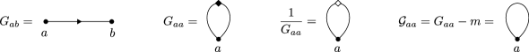
Figure 3.2: The graphical representations of resolvent entries. The versions associated with $G^{*}$ are the same with a dashed line.

We may thus represent the expression on the left-hand side of (3.23), i.e. $Q_{a}({G_{\mu a}G_{a\mu}})Q_{b}({G_{\mu b}^{*}G_{b\mu}^{*}})$, See Figure 3.3; note that our graphical notation does not keep track of the factors $Q$.

Figure 3.3: Graph associated with the monomial $G_{\mu a}G_{a\mu}G_{\mu b}^{*}G_{b\mu}^{*}$. Here we draw the case $a\neq b$.

Having drawn the graph in Figure 3.3, we start making all resolvent entries (corresponding to edges) independent of the indices $a$ and $b$, using the identities (3.13). As explained above, this gives rise to a sum of terms, each one of which is a fraction of resolvent entries that are maximally expanded in $(a,b)$. The denominator of each term contains diagonal resolvent entries, while its numerator is a product of off-diagonal resolvent entries; this follows from the structure of (3.13). A simple such example was given in (3.24). The associated monomial,

$$\frac{G_{\mu b}^{(a)}G_{ba}}{G_{bb}^{(a)}}G_{a\mu}^{(b)}\,\frac{G_{a\mu}^{(b)*}G_{ba}^{*}}{G_{aa}^{(b)*}}G_{\mu b}^{(a)*},$$ (3.25)

may be represented graphically as in Figure 3.4.

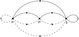
Figure 3.4: Graph associated with (3.25). Here we draw the case $a\neq b$.

We remark that the graphs depicted in Figures 3.3 and 3.4 are fundamentally different in the following sense. In Figure 3.3, each edge of the graph represents a resolvent entry with no upper indices; in Figure 3.4, each edge of the graph represents a resolvent entry that is maximally expanded in $(a,b)$. In the language of Section 6, the former graph will be called $\gamma^{2}(\Delta)$ while the latter will be called $\Gamma$. It is the latter graphs that play a major role in our proofs. The former type is simply a trivial concatenation of basic graphs, and serves as an intermediate step in the construction of graphs of the latter type (i.e. whose edges represent maximally expanded resolvent entries). If one wanted to be more precise, one could keep track of the upper indices associated with each edge in the graphs. By definition, the edges of the graph in Figure 3.3 have no upper indices, and the edges of the graph in Figure 3.4 have upper indices as given in (3.25). However, these upper indices are unambiguously determined by the condition that each resolvent entry be maximally expanded in $(a,b)$. This means that $a$ appears as upper index of any edge that is not incident to $a$ (and similarly with $b$). In practice, however, we do not indicate the upper indices, as they are uniquely determined by the condition that all edges are maximally expanded in $(a,b)$.

It is possible, and indeed important for our proof, to introduce a graphical rule that generates graphs like the one depicted in Figure 3.4 from graphs like the one depicted in Figure 3.3 through a sequence of graphs whose edges are not yet maximally expanded. Before the maximal expansion is achieved, we shall temporarily indicate the upper indices on the graph edges in parenthesis. Recall that the underlying algebra was simply governed by the identities (3.13). Figure 3.5 depicts the identity

$$G_{ij}\;=\;G_{ij}^{(k)}+\frac{G_{ik}G_{kj}}{G_{kk}}\,.$$ (3.26)

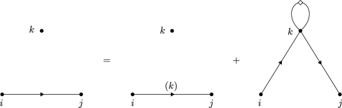
Figure 3.5: The graphical representation of the formula (3.26).

Similarly, the corresponding identities for the diagonal entries,

$$\frac{1}{G_{ii}}\;=\;\frac{1}{G_{ii}^{(j)}}-\frac{G_{ij}G_{ji}}{G_{ii}G_{ii}^{(j)}G_{jj}}\,,\qquad G_{ii}\;=\;G_{ii}^{(j)}+\frac{G_{ij}G_{ji}}{G_{jj}}\,,$$ (3.27)

are depicted in Figure 3.6.

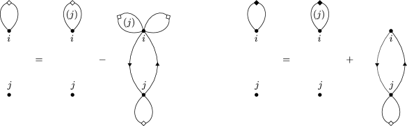
Figure 3.6: Adding an upper index $j$ to the diagonal entries $1/G_{ii}$ and $G_{ii}$. These pictures correspond to (3.27). We exceptionally also mark the upper indices associated with each edge.

Applying the graphical rules of Figures 3.5 and 3.6 to Figure 3.3 results e.g. in Figure 3.4 (and many others). To be precise, we should keep track of the upper indices associated with each edge at each step, as is done in Figure 3.6. When all edges are maximally expanded, we stop the application of the rules of Figures 3.5 and 3.6. However, as explained above, we usually omit the explicit indication of upper indices in graphs after the maximal expansion is achieved. For future use, we record the following definition associated with the operations depicted in Figures 3.5 and 3.6.

Definition 3.10.

We refer to the second graph on the right-hand side of Figure 3.5 as arising from linking the edge $(ij)$ with the vertex $k$. We also say that the vertex $k$ was linked to by the edge $(ij)$. Similarly, in both connected graphs in Figure 3.6, the vertex $j$ was linked to by the edge $(ii)$.

The argument underlying (3.23) may now be formulated graphically as follows. We start from Figure 3.3 and apply the identities from Figures 3.5 and 3.6 until all resolvent entries associated with the edges are maximally expanded in $(a,b)$. Since these identities can be applied in various orders, this procedure is not unique. This lack of uniqueness does not concern us, however: we need only a maximally expanded representation. By the argument given after (3.23), we know that only those graphs in which both $a$ and $b$ have been linked to by an edge survive. Such graphs (as the one from Figure 3.4) have (at least) two additional edges as compared to the one from Figure 3.3. This results in a size $O_{\prec}(\Psi^{6})$.

3.2.3. Sketch of the proof of (B)

We focus first on the first estimate of (3.5). The idea is to derive a stable self-consistent equation for the quantity

$$\frac{1}{N}\sum_{a}^{(\mu)}G_{\mu a}G_{a\mu}\,.$$ (3.28)

We do this by introducing the partition $1=P_{a}+Q_{a}$ inside the summation. The second resulting term was estimated in (A). The first resulting term may be written as

$$\frac{1}{N}\sum_{a}^{(\mu)}P_{a}\bigl{(}{G_{\mu a}G_{a\mu}}\bigr{)} \;=\;\frac{1}{N}\sum_{a}^{(\mu)}P_{a}\biggl{(}{\frac{m^{2}}{G_{aa}^{2}}G_{\mu a}G_{a\mu}}\biggr{)}+O_{\prec}(\Psi^{3})$$

$$\;=\;m^{2}\,\frac{1}{N}\sum_{a}^{(\mu)}P_{a}\biggl{(}{\sum_{x,y}^{(a)}G_{\mu x}^{(a)}h_{xa}h_{ay}G_{y\mu}^{(a)}}\biggr{)}+O_{\prec}(\Psi^{3})$$

$$\;=\;m^{2}\,\frac{1}{N}\sum_{a}^{(\mu)}\sum_{x}^{(a)}s_{ax}G_{\mu x}^{(a)}G_{x\mu}^{(a)}+O_{\prec}(\Psi^{3})$$

$$\;=\;m^{2}\,\frac{1}{N}\sum_{a}^{(\mu)}\sum_{x}^{(a)}s_{ax}G_{\mu x}G_{x\mu}+O_{\prec}(\Psi^{3})$$

$$\;=\;m^{2}\,\frac{1}{N}\sum_{x}^{(\mu)}G_{\mu x}G_{x\mu}+O_{\prec}(\Psi^{3}+N^{-1})\,.$$

In the first step we used (3.17). In the second step we used the identity (3.14a) (note the usefulness of smuggling in $G_{aa}$ in the previous step). In the third step we used the identity $P_{a}h_{xa}h_{ay}=\mathbb{E}h_{xa}h_{ay}=s_{ax}\delta_{xy}$, as follows from the definition of $H$ and the fact that $G^{(a)}$ is independent of $a$. In the fourth step we used the identity (3.13) to remove the upper indices. In the fifth step we used a simple analysis of coinciding indices together with the estimates (2.2) and (3.11). Together with the bound from (A), we therefore get for the quantity (3.28) the self-consistent equation

$$\frac{1}{N}\sum_{a}^{(\mu)}G_{\mu a}G_{a\mu} \;=\;\frac{1}{N}\sum_{a}^{(\mu)}P_{a}\bigl{(}{G_{\mu a}G_{a\mu}}\bigr{)}+O_{\prec}(\Psi^{3})$$

$$\;=\;m^{2}\frac{1}{N}\sum_{x}^{(\mu)}G_{\mu x}G_{x\mu}+O_{\prec}\bigl{(}{\Psi^{3}+M^{-1}}\bigr{)}$$

$$\;=\;m^{2}\frac{1}{N}\sum_{x}^{(\mu)}G_{\mu x}G_{x\mu}+O_{\prec}\Bigl{(}{\Psi^{2}\bigl{(}{\Psi+M^{-1/2}\Psi^{-1}}\bigr{)}}\Bigr{)}\,,$$

where in the last step we used (2.9). Using (3.4) and the trivial bound $\frac{1}{N}\sum_{a}^{(\mu)}G_{\mu a}G_{a\mu}\prec\Psi^{2}$ we therefore get

$$\frac{1}{N}\sum_{a}^{(\mu)}G_{\mu a}G_{a\mu}\;\prec\;\min\biggl{\{}{\Psi^{2}\,,\,\frac{\Psi^{2}\bigl{(}{\Psi+M^{-1/2}\Psi^{-1}}\bigr{)}}{|1-m^{2}|}}\biggr{\}}\;\leqslant\;\min\bigl{\{}{\Psi^{2}\,,\,\varrho\Psi^{2}\bigl{(}{\Psi+M^{-1/2}\Psi^{-1}}\bigr{)}}\bigr{\}}\;=\;\Psi^{2}\Phi\,,$$

which is the first estimate of (3.5).

The proof of the first estimate of (3.7) is similar, except that we derive the self-consistent equation using (3.14c) instead of (3.14a). Using the second estimate of (3.7) we find

$$\frac{1}{N}\sum_{a}(G_{aa}-m)\;=\;\frac{1}{N}\sum_{a}P_{a}(G_{aa}-m)+\frac{1}{N}\sum_{a}Q_{a}G_{aa}\;=\;\frac{1}{N}\sum_{a}P_{a}(G_{aa}-m)+O_{\prec}(\Psi^{2})\,.$$ (3.29)

Next, from a simple large deviation estimate (see the first paragraph in the proof of Lemma 9.1 in Appendix A) we find $Z_{a}\prec\Psi$. Moreover, Lemma 3.8, (2.3), (2.2), and (2.9) readily imply that $U_{a}^{(a)}\prec\Psi$. Recalling the estimate (2.10), we may therefore expand the identity (3.14c) using (2.7) to get

$$G_{aa}\;=\;m+m^{2}(-h_{aa}+Z_{a}+U_{a}^{(a)})+O_{\prec}(\Psi^{2})\,.$$

Using $P_{a}h_{aa}=0$ and $P_{a}Z_{a}=0$ we therefore find

$$\frac{1}{N}\sum_{a}P_{a}(G_{aa}-m) \;=\;m^{2}\frac{1}{N}\sum_{a}P_{a}U_{a}^{(a)}+O_{\prec}(\Psi^{2})$$

$$\;=\;m^{2}\frac{1}{N}\sum_{a}\sum_{x}^{(a)}s_{ax}(G_{xx}^{(a)}-m)+O_{\prec}(\Psi^{2})$$

$$\;=\;m^{2}\frac{1}{N}\sum_{x}(G_{xx}-m)+O_{\prec}(\Psi^{2})\,,$$

where in the second step we recalled the definition (3.15) and used (2.2) as well as (2.3) to write $m=\sum_{x}^{(a)}s_{ax}m+O(M^{-1})$ with $M^{-1}=O(\Psi^{2})$ by (2.9), and in the third (3.13) to get rid of the upper index $a$ as well as (2.3). Thus, together with (3.29), we get the self-consistent equation

$$\frac{1}{N}\sum_{a}(G_{aa}-m)\;=\;m^{2}\frac{1}{N}\sum_{x}(G_{xx}-m)+O_{\prec}(\Psi^{2})\,,$$ (3.30)

from which we easily conclude the first estimate of (3.7) as before.

In both of the above examples the averaging was performed with respect to the uniform weight $w_{a}=N^{-1}$. We conclude by sketching the differences in the case of a nontrivial weight, e.g. $w_{a}=s_{\nu a}$. Consider for example the average $\sum_{a}s_{\nu a}(G_{aa}-m)$ from (3.8). Repeating the above derivation of (3.30), we find the self-consistent system of equations

$$\sum_{a}s_{\nu a}(G_{aa}-m)\;=\;m^{2}\sum_{a}s_{\nu a}\sum_{x}s_{ax}(G_{xx}-m)+E_{\nu}\,$$

for each $\nu$. Here the error satisfies $E_{\nu}=O_{\prec}(\Psi^{2})$. Introducing the vectors $\bm{\mathrm{v}}=(v_{a})_{a=1}^{N}$ defined by $v_{a}\mathrel{\vbox{\hbox{.}\hbox{.}}}=\sum_{x}s_{ax}(G_{xx}-m)$ and $\bm{\mathrm{E}}=(E_{\nu})_{\nu=1}^{N}$, we have

$$\bm{\mathrm{v}}\;=\;m^{2}S\bm{\mathrm{v}}+{\bm{\mathrm{E}}}\,.$$

Thus we find

$$\bm{\mathrm{v}}\;=\;(1-m^{2}S)^{-1}{\bm{\mathrm{E}}}\,,$$

from which we conclude that $v_{a}\prec\varrho\Psi^{2}\leqslant\Psi\Phi$.

3.2.4. Sketch of the proof of (C)

As in (A), the proof is based on a high-moment estimate. We again restrict our attention to the variance

$$\mathbb{E}\biggl{\lvert}\frac{1}{N}\sum_{a}^{(\mu)}Q_{a}(G_{\mu a}G_{a\mu}^{*})\biggr{\rvert}^{2}\;=\;\frac{1}{N^{2}}\sum_{a,b}^{(\mu)}\mathbb{E}\,Q_{a}(G_{\mu a}G_{a\mu}^{*})\,Q_{b}(G_{\mu b}G_{b\mu}^{*})\,.$$ (3.31)

Our goal is to derive the stochastic bound $\Psi^{6}\Phi^{2}$ for (3.31). The case $a=b$ yields the bound

$$\frac{1}{N^{2}}\sum_{a}^{(\mu)}\lvert G_{\mu a}\rvert^{4}\;\prec\;\Psi^{4}N^{-1}\;\leqslant\;\Psi^{6}\Phi^{2}\,.$$ (3.32)

Let us therefore assume for the following that $a\neq b$. The first part of the argument follows precisely the proof of (A) above. We expand all resolvent entries of

$$\mathbb{E}\,Q_{a}(G_{\mu a}G_{a\mu}^{*})\,Q_{b}(G_{\mu b}G_{b\mu}^{*})$$ (3.33)

using (3.13) and obtain a sum of monomials whose resolvent entries are maximally expanded in $(a,b)$. A typical example of a nonvanishing term arising from the expansion of (3.31) is

$$\mathbb{E}\,Q_{a}\Biggl{(}{\frac{G_{\mu b}^{(a)}G_{ba}}{G_{bb}^{(a)}}G_{a\mu}^{(b)*}}\Biggr{)}\,Q_{b}\Biggl{(}{G_{\mu b}^{(a)}\frac{G_{ba}^{*}G_{a\mu}^{(b)*}}{G_{aa}^{(a)*}}}\Biggr{)}\,.$$

As in the proof of (A), this immediately gives the stochastic bound $\Psi^{6}$. See Figure 3.7 for a graphical summary of the argument in this context.

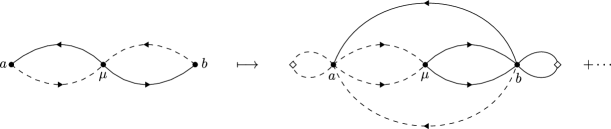
Figure 3.7: The process of making all edges of the graph associated with (3.33) maximally expanded in $(a,b)$.

The bound $\Psi^{6}$ is not enough, however. In order to improve this to $\Psi^{6}\Phi^{2}$, we introduce a new operation which we call vertex resolution. In order to simplify the presentation, in the following we systematically replace any diagonal entry $G_{aa}^{(T)}$ by $m$. The resulting error terms are small by definition of $\Lambda$ (of course, they have to be dealt with, which is done Section 9.1 of the full proof below). Thus, we have to estimate the expression

$$\mathbb{E}\,Q_{a}\bigl{(}{G_{\mu b}^{(a)}G_{ba}G_{a\mu}^{(b)*}}\bigr{)}\,Q_{b}\bigl{(}{G_{\mu b}^{(a)}G_{ba}^{*}G_{a\mu}^{(b)*}}\bigr{)}$$ (3.34)

for $a\neq b$. We begin by expanding all resolvent entries using the Family B identity (3.14a), again neglecting the diagonal prefactors in (3.14a). This gives

$$\sum_{x,y,z,w}^{(ab)}\sum_{x^{\prime},y^{\prime},z^{\prime},w^{\prime}}^{(ab)}\mathbb{E}\,Q_{a}\bigl{(}{G_{\mu x}^{(ab)}h_{xb}h_{by}G_{yz}^{(ab)}h_{za}h_{aw}G_{w\mu}^{(ab)*}}\bigr{)}\,Q_{b}\bigl{(}{G_{\mu x^{\prime}}^{(ab)}h_{x^{\prime}b}h_{by^{\prime}}G_{y^{\prime}z^{\prime}}^{(ab)*}h_{z^{\prime}a}h_{aw^{\prime}}G_{w^{\prime}\mu}^{(ab)*}}\bigr{)}\,.$$ (3.35)

(Here we also ignored a few special cases of coinciding indices when expanding both $a$ and $b$ in $G_{ab}$ using (3.14a). As usual, the resulting terms are subleading and unimportant for this sketchy discussion.) The idea behind (3.35) is to expand all of the randomness that depends on $a$ and $b$ explicitly (i.e. in entries of $H$), so that partial expectations may be explicitly taken. Note that all resolvent entries in (3.35) are independent of $a$ and $b$. We may now take the expectation $\mathbb{E}$ in (3.35); more precisely, we reorganize (3.35) as

$$\sum_{x,y,z,w}^{(ab)}\sum_{x^{\prime},y^{\prime},z^{\prime},w^{\prime}}^{(ab)}\mathbb{E}\,G_{\mu x}^{(ab)}G_{yz}^{(ab)}G_{w\mu}^{(ab)*}G_{\mu x^{\prime}}^{(ab)}G_{y^{\prime}z^{\prime}}^{(ab)*}G_{w^{\prime}\mu}^{(ab)*}\,P_{a}\Bigl{[}{Q_{a}(h_{za}h_{aw})h_{z^{\prime}a}h_{aw^{\prime}}}\Bigr{]}P_{b}\Bigl{[}{h_{xb}h_{by}Q_{b}(h_{x^{\prime}b}h_{by^{\prime}})}\Bigr{]}\,.$$ (3.36)

The two square brackets in (3.35) may be computed explicitly. Since $\mathbb{E}h_{uv}=0$, each matrix entry $h_{uv}$ must (at least) be paired with another copy of the same factor or its conjugate $\bar{h}_{uv}=h_{vu}$. Assume first that we are dealing with a complex Hermitian band matrix (condition (3.21)). In that case, each $h_{uv}$ must be paired with its conjugate $h_{vu}$ since $\mathbb{E}h_{uv}^{2}=0$. Of course, it may happen that more than two entries have coinciding indices, but this leads to a term that is subleading by a factor $M^{-1/2}$, and which we neglect here. Thus, $h_{za}$ in (3.36) may be paired with $h_{aw}$ (resulting in $z=w$) or with $h_{aw^{\prime}}$ (resulting in $z=w^{\prime}$). However, the pairing $h_{za}$ with $h_{aw}$ gives a vanishing contribution owing to the presence of $Q_{a}$, since

$$\mathbb{E}_{za}Q_{a}(h_{za}h_{az})\;=\;0$$

where $\mathbb{E}_{za}$ denotes partial expectation with respect to $h_{za}$. In other words, $Q_{a}$ forbids the pairing of $h_{za}$ with $h_{aw}$, and similarly $Q_{b}$ the pairing of $h_{x^{\prime}b}$ with $h_{by^{\prime}}$. Thus the leading order term resulting from the square brackets in (3.36), on which we focus here, is the pairing

$$s_{az}s_{aw}s_{bx}s_{by}\,\delta_{wz^{\prime}}\delta_{zw^{\prime}}\delta_{x^{\prime}y}\delta_{xy^{\prime}}\,.$$ (3.37)

In the real symmetric case (condition (3.20)), where $\mathbb{E}h_{uv}^{2}$ does not vanish, $h_{za}$ can also be paired with $h_{z^{\prime}a}$. (Note that $Q_{a}$ still forbids the pairing of $h_{za}$ with $h_{aw}$.) This yields the three further allowed pairings

$$s_{az}s_{aw}s_{bx}s_{by}\delta_{zz^{\prime}}\delta_{ww^{\prime}}\delta_{x^{\prime}y}\delta_{xy^{\prime}}\,,\qquad s_{az}s_{aw}s_{bx}s_{by}\delta_{wz^{\prime}}\delta_{zw^{\prime}}\delta_{xx^{\prime}}\delta_{yy^{\prime}}\,,\qquad s_{az}s_{aw}s_{bx}s_{by}\delta_{zz^{\prime}}\delta_{ww^{\prime}}\delta_{xx^{\prime}}\delta_{yy^{\prime}}\,.$$ (3.38)

Assuming again condition (3.21), only (3.37) contributes, and we get the expression (up to lower order error terms in $M^{-1/2}$)

$$\sum_{x,y,z,w}^{(ab)}s_{bx}s_{by}s_{az}s_{aw}\,\mathbb{E}\,G_{\mu x}^{(ab)}G_{yz}^{(ab)}G_{w\mu}^{(ab)*}G_{\mu y}^{(ab)}G_{xw}^{(ab)*}G_{z\mu}^{(ab)*}\\ =\;\mathbb{E}\Biggl{(}{\sum_{x,w}s_{aw}s_{bx}G_{\mu x}^{(ab)}G_{xw}^{(ab)*}G_{w\mu}^{(ab)*}}\Biggr{)}\Biggl{(}{\sum_{y,z}s_{by}s_{az}G_{\mu y}^{(ab)}G_{yz}^{(ab)}G_{z\mu}^{(ab)*}}\Biggr{)}\,.$$ (3.39)

Now each of the expressions in the parentheses is stochastically bounded by $\Psi^{3}\Phi$. Indeed, an argument very similar to the proof of (B) above yields

$$\sum_{y}s_{by}G_{\mu y}^{(ab)}G_{yz}^{(ab)}\;\prec\;\Psi^{2}\Phi\,.$$ (3.40)

(The additional upper indices $(ab)$ are unimportant.) Thus, from the summation over $y$ in (3.39) we gain an additional factor $\Phi$ (and, similarly, from the summation over $w$). We therefore find that (3.33) is stochastically bounded by $\Psi^{6}\Phi^{2}$, which was the claim of (C).

The use of graphs greatly clarifies the mechanism underlying the above sketch of the proof of (C). In order to depict vertex resolution, we need a graphical notation for edges associated with matrix entries $h_{uv}$ and $s_{ab}$; we represent the former using dotted lines and the latter using wiggly lines. See Figure 3.8.

Figure 3.8: The graphical notation for entries of $G$, $G^{*}$, $H$, and $S$. Since $S$ is symmetric, the edge associated with $s_{ab}$ is undirected.

As seen above, the starting point for the operation of vertex resolution is (3.34). The expanded expression (3.35) may be graphically represented as in Figure 3.9. Thus, the vertex $a$ is “resolved” into four (i.e. the degree of $a$) new vertices, which are drawn in white and are connected to their parent vertex $a$ by dotted lines (corresponding to a matrix entry of $H$). White vertices are either incoming or outgoing, depending on the orientation of the dotted edge that joins them to their parent vertex $a$. Similarly, the vertex $b$ is resolved into four new vertices.

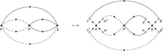
Figure 3.9: Resolving the vertices $a$ and $b$. In accordance with (3.35), we ignore the loops associated with diagonal terms. (These lead to corrections that are higher order in $\Psi$.)

Note that each solid or dashed edge in the right-hand graph of Figure 3.9 represents a resolvent matrix entry that is independent of $a$ and $b$. The expression (3.39) was obtained from (3.35) by computing the partial expectations $P_{a}$ and $P_{b}$ of the associated entries of $H$. Graphically, this amounts to a pairing of the white vertices surrounding each black parent vertex. (Note that the factors $Q$, which yielded constraints on the allowed pairings, are not visible in the graphs. This is not a problem, however, as the ensuing bounds will hold for all pairings, even if these restrictions are relaxed.) The pairing of two dotted lines gives rise to a wiggly line, in accordance with the identity $\mathbb{E}_{a}\lvert h_{ax}\rvert^{2}=s_{ax}$. See Figure 3.10 for a graphical representation of the pairing in (3.39). In Figure 3.10 we represented the pairing (3.37), which is the only one in the complex Hermitian case (3.21). In this case, the orientation of the edges must be matched when pairing white vertices, i.e. an incoming white vertex can only be paired with an outgoing one. This is an immediate consequence of the condition $\mathbb{E}h_{ax}^{2}=0$, as explained after (3.37). In the real symmetric case (3.20), where $\mathbb{E}_{a}\lvert h_{ax}\rvert^{2}=\mathbb{E}h_{ax}^{2}=s_{ax}$, the other pairings (3.38) are also possible. Graphically, this means that, when pairing white vertices, there are no constraints on the orientation of the incident edges. In other words, the arrows on the dotted edges may be ignored.

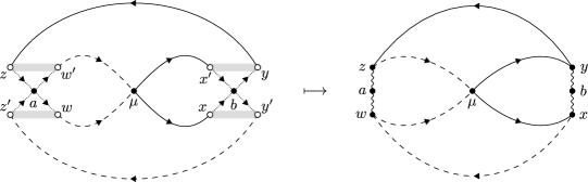
Figure 3.10: Taking a pairing of the white vertices to get the completed resolution.

The result of the vertex resolution is graphically evident when comparing the first graph in Figure 3.9 and second graph of Figure 3.10: the vertex $a$, of degree four, has been split (or “resolved”) into two vertices of degree two. (The same happened for $b$). This resolution also entails the creation of new summation indices, $z$ and $w$. Each one of them is connected to the original vertex $a$ by a factor $s_{az}$ (respectively $s_{aw}$), which implies that the summation over the larger family of summation indices is still performed with respect to a normalized weight. Generally, vertex resolution splits vertices of high degree into several vertices of degree two. The reason why this helps is that we can gain an extra factor $\Phi$ from any summation vertex of degree two whose incident edges are of the same “colour” (solid or dashed). We shall use the name marked vertex (see Definition 8.1 below) to denote a vertex whose resolution yields at least one new summation vertex whose (two) incident edges are of the same colour. The mechanism behind the gain of a factor $\Phi$ from a newly created (via resolution) index is roughly the content of (B), and was used in (3.40). In our case, we gain from the summations over $y$ and $w$ (but not $z$ or $x$). Generally, the process of vertex resolution yields long “chains” (i.e. subgraphs whose vertices have degree two), each vertex of which yields an extra factor $\Phi$ provided both incident edges have the same colour. In fact, establishing such estimates for chains is an important step in our proof (see Proposition 5.3 below). This concludes our overview of the proof of Proposition 3.3.

4 General monomials and main result

In this section we state the fluctuation averaging theorem in full generality. To that end, we introduce a general class of monomials which we shall average. We consider monomials in the variables

$$\mathcal{G}_{ij}(z)\;\mathrel{\vbox{\hbox{.}\hbox{.}}}=\;G_{ij}(z)-\delta_{ij}m(z)\,,$$

which yield a more consistent power counting for diagonal resolvent entries. Indeed, by definition $\lvert\mathcal{G}_{ij}\rvert\leqslant\Lambda$ for all $i$ and $j$. As we saw in Section 3, monomials in the resolvent entries are best described using graphs; see (3.10) and Figure 3.1.

We may now define the graphs $\Delta$ used to describe monomials.

Definition 4.1 (Admissible graphs).

1. Let $V_{s}$ and $V_{e}$ be finite disjoint sets. Let $V\mathrel{\vbox{\hbox{.}\hbox{.}}}=V_{s}\sqcup V_{e}$ be their disjoint union and $E$ be a subset of the ordered pairs $V\times V$. The quadruple

   $$\Delta\;=\;(V_{s},V_{e},E,\xi)$$

   is an admissible graph if it is a directed, edge-coloured, multigraph with set of vertices $V$. The edges are ordered pairs of vertices with multiplicity, i.e. we allow loops and multiple edges. We shall also use the notation $V_{s}\equiv V_{s}(\Delta)$, $V_{e}\equiv V_{e}(\Delta)$, and $E\equiv E(\Delta)$.

   More formally, we can view $E(\Delta)$ as an arbitrary finite set equipped with maps $\alpha,\beta\mathrel{\vbox{\hbox{.}\hbox{.}}}E(\Delta)\to V(\Delta)$. Here $\alpha(e)$ and $\beta(e)$ represent the source and target vertices of the edge $e\in E(\Delta)$. The colouring $\xi\mathrel{\vbox{\hbox{.}\hbox{.}}}E(\Delta)\to\{1,*\}$ is a mapping that assigns one of two “colours”, $1$ or $*$, to each edge. If no confusion is possible with the multiplicity of an edge $e\in E(\Delta)$, we shall identify it with the ordered pair $(\alpha(e),\beta(e))$.

2. We denote by $\mathfrak{Z}$ the set of admissible graphs $\Delta$ on arbitrary $V_{s}$ and $V_{e}$.

3. The degree of $\Delta\in\mathfrak{Z}$ is

   $$\deg(\Delta)\;\mathrel{\vbox{\hbox{.}\hbox{.}}}=\;\lvert E(\Delta)\rvert\,.$$

The set $V_{s}(\Delta)$ will label the family of summation indices ($(a,b)=(a_{i})_{i\in V_{s}(\Delta)}$ in the example (3.9)), and $V_{e}(\Delta)$ the set of external indices ($(\mu,\nu)=(\mu_{i})_{i\in V_{e}(\Delta)}$ in the example (3.9)). We use the notation

$$\bm{\mathrm{u}}\;=\;(\bm{\mathrm{a}},\bm{\mathrm{\mu}})\,,\qquad\bm{\mathrm{a}}\;=\;(a_{i})_{i\in V_{s}(\Delta)}\,,\qquad\bm{\mathrm{\mu}}\;=\;(\mu_{i})_{i\in V_{e}(\Delta)}$$ (4.1)

for the matrix indices. Generally, we try to use Latin letters $a,b,c,d,x,y,z,\dots$ for summation indices and Greek letters $\mu,\nu\,\dots$ for external indices.

Although our statements and proofs hold for any admissible graph $\Delta$, in order to avoid trivial cases in our applications we shall always consider graphs without isolated vertices and with the property that each edge is incident to at least one vertex $V_{s}(\Delta)$, i.e. every resolvent entry contains at least one summation index.

Next, we introduce the monomials in $(\mathcal{G}_{xy})$ whose average we shall estimate.

Definition 4.2 (Monomials).

Let $\Delta\in\mathfrak{Z}$ be an admissible graph and let $\bm{\mathrm{\mu}}\in\{1,\dots,N\}^{V_{e}(\Delta)}$ be a collection of external indices. We define the monomial

$$\mathcal{Z}_{\bm{\mathrm{a}}}\;\equiv\;\mathcal{Z}_{\bm{\mathrm{a}}}^{\bm{\mathrm{\mu}}}(\Delta)\;\mathrel{\vbox{\hbox{.}\hbox{.}}}=\;\prod_{e\in E(\Delta)}\mathcal{G}_{u_{\alpha(e)}u_{\beta(e)}}^{\xi_{e}}\,$$ (4.2)

which is regarded as a function of the summation indices $\bm{\mathrm{a}}$, recalling the splitting of the indices (4.1). We also denote by

$$\mathcal{Z}\;=\;\bigl{(}{\mathcal{Z}_{\bm{\mathrm{a}}}^{\bm{\mathrm{\mu}}}(\Delta)\mathrel{\vbox{\hbox{.}\hbox{.}}}\bm{\mathrm{a}}\in\{1,\dots,N\}^{V_{s}(\Delta)}}\bigr{)}$$

the family of monomials associated with $(\Delta,\bm{\mathrm{\mu}})$ by (4.2), and say that $\Delta$ encodes the monomial $\mathcal{Z}_{\bm{\mathrm{a}}}$.

Note that $\deg(\Delta)$ is the degree of the monomial $\mathcal{Z}_{\bm{\mathrm{a}}}$ encoded by $\Delta$. Throughout the following we shall frequently drop the explicit dependence of $\mathcal{Z}_{\bm{\mathrm{a}}}$ on $\bm{\mathrm{\mu}}$ and $\Delta$.

The averaging over $\bm{\mathrm{a}}$ will be performed with respect to a weight $w(\bm{\mathrm{a}})$. In the example (3.9), this weight was $w(a,b)=s_{\mu a}s_{\rho b}$. A typical example of a weight is

$$w(a,b,c)\;=\;\frac{1}{N}\sum_{d}s_{\mu d}s_{db}s_{bc}\,\qquad\mbox{for}\quad\bm{\mathrm{a}}=(a,b,c)\,.$$ (4.3)

In order to define a general class of weights, the following notion of partitioning of summation indices is helpful.

Definition 4.3 (Partition of indices).

Let $I$ be a finite index set. For $\bm{\mathrm{a}}=(a_{i})_{i\in I}\in\{1,\dots,N\}^{I}$ we denote by $\mathcal{P}(\bm{\mathrm{a}})$ the partition of $I$ defined by the equivalence relation $k\sim l$ if and only if $a_{k}=a_{l}$.

Generally, we consider weights satisfying the following definition; when reading it, it is good to keep examples of the type (4.3) in mind.

Definition 4.4 (Weights).

A map $w\mathrel{\vbox{\hbox{.}\hbox{.}}}\{1,\dots,N\}^{V_{s}(\Delta)}\to[0,1]$ is a weight adapted to $\Delta\in\mathfrak{Z}$ if it satisfies the following condition. Let $V_{s}(\Delta)=I\sqcup J$ be a (possibly trivial) partition of $V_{s}(\Delta)$ into two disjoint subsets, inducing a splitting $\bm{\mathrm{a}}=(\bm{\mathrm{a}}_{I},\bm{\mathrm{a}}_{J})$ of the summation indices. Then we require that, for any partition $P$ of $J$, we have

$$\max_{\bm{\mathrm{a}}_{I}}\sum_{\bm{\mathrm{a}}_{J}}\bm{\mathrm{1}}\bigl{(}{\mathcal{P}(\bm{\mathrm{a}}_{J})=P}\bigr{)}\,w(\bm{\mathrm{a}}_{I},\bm{\mathrm{a}}_{J})\;\leqslant\;M^{\lvert P\rvert-\lvert V_{s}(\Delta)\rvert}\,,$$ (4.4)

where $\lvert P\rvert$ denotes the number of blocks in $P$.

The interpretation of (4.4) is that the left-hand side of (4.4) has $\lvert P\rvert$ free summation indices; the remaining summation indices have been either frozen (i.e. they belong to $\bm{\mathrm{a}}_{I}$) or merged with others (i.e. they belong to a nontrivial block of $P$). Then (4.4) simply states that each suppressed summation yields a factor $M^{-1}$. In particular, with $J=V_{s}(\Delta)$ and the trivial atomic partition $P$ we have

$$\sum_{\bm{\mathrm{a}}}w(\bm{\mathrm{a}})\;\leqslant\;1\,,$$

i.e. the total sum of all weights is always bounded by one.

When estimating averages such as (3.9), we shall always impose that all indices that have distinct names also have distinct values. In the case that two indices have the same value, we give them the same name. Thus, for example we write

$$\frac{1}{N^{2}}\sum_{a,b}G_{\mu a}G_{ab}G_{b\mu}\\ =\;\frac{1}{N^{2}}\sum_{a,b}^{(\mu)*}G_{\mu a}G_{ab}G_{b\mu}+\frac{1}{N^{2}}\sum_{a}^{(\mu)}G_{\mu a}G_{aa}G_{a\mu}+\frac{1}{N^{2}}\sum_{a}^{(\mu)}G_{\mu a}G_{a\mu}G_{\mu\mu}+\frac{1}{N^{2}}\sum_{b}^{(\mu)}G_{\mu\mu}G_{\mu b}G_{b\mu}+\frac{1}{N^{2}}G_{\mu\mu}^{3}\,,$$

where a star on top of a summation means that all summation indices are constrained to be distinct. (Recall also the notation $\sum^{(S)}$ for $S\subset\{1,\dots,N\}$ from Definition 2.2.)

We may now define our central quantity. Let $\Delta\in\mathfrak{Z}$ and $\bm{\mathrm{\mu}}\in\{1,\dots,N\}^{V_{e}(\Delta)}$ be a collection of external indices. Let $F\subset V_{s}(\Delta)$ and $w$ be a weight adapted to $\Delta$. We define

$$X_{F}^{w}(\Delta)\;\equiv\;X_{F}^{w,\bm{\mathrm{\mu}}}(\Delta)\;\mathrel{\vbox{\hbox{.}\hbox{.}}}=\;\sum_{\bm{\mathrm{a}}}^{(\bm{\mathrm{\mu}})*}w(\bm{\mathrm{a}})\,\Biggl{[}{\prod_{i\in F}Q_{a_{i}}}\Biggr{]}\mathcal{Z}_{\bm{\mathrm{a}}}^{\bm{\mathrm{\mu}}}(\Delta)\,.$$ (4.5)

Thus, $F$ denotes the set of summation indices that come with an operator $Q$. As explained above, the symbol $(\bm{\mathrm{\mu}})$ on top of them sum means that $a_{i}\neq\mu_{j}$ for all $i\in V_{s}(\Delta)$ and $j\in V_{e}(\Delta)$, and the star means that $a_{i}\neq a_{j}$ for all distinct $i,j\in V_{s}(\Delta)$. Throughout the following, we shall frequently drop the explicit dependence of $X_{F}^{w,\bm{\mathrm{\mu}}}(\Delta)$ on $\bm{\mathrm{\mu}}$.

Remark 4.5.

In (4.5) each operator $Q$ acts on all resolvent entries in $\mathcal{Z}_{\bm{\mathrm{a}}}$. We make this choice to simplify the presentation; also, this is sufficient for all of our current applications. However, our results may be easily extended to more complicated quantities, in which each $Q$ acts only on a subset of the resolvent entries in $\mathcal{Z}_{\bm{\mathrm{a}}}$. Thus, in general, there a resolvent entry is either outside or inside $Q_{a_{i}}$, for each $i\in F$. We require that each resolvent entry outside $Q_{a_{i}}$ have no index $a_{i}$, and at least one resolvent entry inside $Q_{a_{i}}$ have an index $a_{i}$. Then our proof carries over with merely cosmetic changes. For example, expressions such as

$$\sum_{a,b,c,d}^{(\mu\nu)*}s_{\mu a}s_{\rho b}s_{bc}\,Q_{a}\Bigl{(}{G_{\mu a}Q_{b}(G_{ab}G^{*}_{b\nu})Q_{c}(G^{*}_{ac}G_{cd})G_{d\mu}}\Bigr{)}$$

may be estimated in this fashion.

From Lemmas 3.6 and 3.9, we find the trivial bound

$$X^{w}_{F}(\Delta)\;\prec\;\Psi^{\deg(\Delta)}$$ (4.6)

for any adapted weight $w$, provided that $\Lambda\prec\Psi$. We call (4.6) trivial because we also have the bound

$$\mathcal{Z}_{\bm{\mathrm{a}}}^{\bm{\mathrm{\mu}}}(\Delta)\;\prec\;\Psi^{\deg(\Delta)}\,.$$

Hence the estimate (4.6) has not been improved by the averaging over $\bm{\mathrm{a}}$.

Next, we define indices which count the gain in the size of $X_{F}^{w}(\Delta)$ resulting from the averaging over $\bm{\mathrm{a}}$ and from the factors $Q$.

Definition 4.6.

Let $\Delta$ be an edge-coloured graph as in Definition 4.1. For $i\in V(\Delta)$ we set

$$\nu_{i}(\Delta) \;\mathrel{\vbox{\hbox{.}\hbox{.}}}=\;\sum_{(j,k)\in E(\Delta)}\bm{\mathrm{1}}(\xi_{(j,k)}=1)\Bigl{[}{\bm{\mathrm{1}}(i=j)+\bm{\mathrm{1}}(i=k)}\Bigr{]}\,,$$

$$\nu_{i}^{*}(\Delta) \;\mathrel{\vbox{\hbox{.}\hbox{.}}}=\;\sum_{(j,k)\in E(\Delta)}\bm{\mathrm{1}}(\xi_{(j,k)}=*)\Bigl{[}{\bm{\mathrm{1}}(i=j)+\bm{\mathrm{1}}(i=k)}\Bigr{]}\,.$$

Informally, $\nu_{i}(\Delta)$ is the number of legs of colour $1$ incident to $i$, and $\nu_{i}^{*}(\Delta)$ the number of legs of colour $*$ incident to $i$.

We shall use $\deg(i)\equiv\deg_{\Delta}(i)$ to denote the degree of the vertex $i\in V(\Delta)$. It is sometimes important to emphasize that this degree is computed with respect to the graph $\Delta$, which we indicate using the subscript $\Delta$. By definition, $\deg_{\Delta}(i)$ is the number of legs incident to $i$, i.e. a loop at $i$ counts twice. In particular, $\deg_{\Delta}(i)=\nu_{i}(\Delta)+\nu_{i}^{*}(\Delta)$.

In terms of the monomials $\mathcal{Z}$ encoded by $\Delta$, the index $\nu_{i}(\Delta)$ (respectively $\nu_{i}^{*}(\Delta)$) is the number of resolvent entries of $\mathcal{G}$ (respectively of $\mathcal{G}^{*}$) in which the index $a_{i}$ appears. (Note that if the index $a_{i}$ appears twice in a resolvent entry, this entry is counted twice.)

Definition 4.7 (Charged vertex).

We call a summation vertex $i\in V_{s}(\Delta)$ charged if either

1. $i\notin F$ and $\nu_{i}\neq\nu_{i}^{*}$, or

2. $i\in F$ and $\lvert\nu_{i}-\nu_{i}^{*}\rvert\neq 2$.

We denote by $V_{c}(\Delta)\subset V_{s}(\Delta)$ the set of charged vertices.

We may now state our main result.

Theorem 4.8 (Averaging theorem).

Suppose that $\Lambda\prec\Psi$ for some admissible control parameter $\Psi$. Let $\Delta\in\mathfrak{Z}$ (recall Definitions 4.1 and 4.2) and $F\subset V_{s}(\Delta)$. Then

$$X_{F}^{w,\bm{\mathrm{\mu}}}(\Delta)\;\prec\;\Psi^{\deg(\Delta)+\lvert F\rvert}\,\Phi^{\lvert V_{c}(\Delta)\rvert}$$ (4.7)

for any $\bm{\mathrm{\mu}}$ and weight $w$ adapted to $\Delta$ (recall Definition 4.4).

Thus, Theorem 4.8 states that we gain a factor $\Psi$ from each $Q$ and a factor $\Phi$ from each charged vertex. The rationale behind the name “charged” is that, in the vertex resolution process from the proof of Theorem 4.8, a charged vertex gives rise, in leading order, to a collection vertices of degree two, at least one of which will be a chain vertex (see Definition 5.1) and hence yield a factor $\Phi$ using the a priori bounds of Section 7.

Remark 4.9.

The right-hand side of (4.7) can be estimated from above by

$$(\Psi+M^{-1/4})^{\deg(\Delta)+\lvert F\rvert+\lvert V_{c}(\Delta)\rvert}\,,$$

which gives a simple power counting in terms of the quantity $\Psi+M^{-1/4}$. From each summation index $a_{i}$ without an associated $Q_{a_{i}}$ we gain a factor $\Psi+M^{-1/4}$ if $\nu_{i}\neq\nu_{i}^{*}$. If there is a $Q_{a_{i}}$ then we gain at least a factor $\Psi+M^{-1/4}$, and, provided that $\lvert\nu_{i}-\nu_{i}^{*}\rvert\neq 2$, one additional factor $\Psi+M^{-1/4}$. Note that we gain at most two additional factors $\Psi+M^{-1/4}$ from each summation index.

Remark 4.10.

As explained after (3.6), the additional term $M^{-1/2}\Psi^{-1}$ in the definition of $\Phi$ is a (necessary) technical nuisance and should be thought of as a lower order term in typical applications. In general, however, it cannot be eliminated, and Theorem 4.8 cannot be formulated in terms of powers of $\Psi$ alone. This may be seen for instance from the variance calculation of the quantity $\frac{1}{N}\sum_{a}^{(\mu)}Q_{a}(G_{\mu a}G_{a\mu}^{*})$. Indeed, as is apparent from (3.32), the term arising from $a=b$ is of order $N^{-1}\Psi^{4}$, which is in general not bounded by $\Psi^{8}$.

Remark 4.11.

The requirement that (2.5) hold for all $p$ can be easily relaxed. Indeed, Theorem 4.8 has the following variant. Fix $\varepsilon>0$ and $D>0$. Then there exists a $p(\varepsilon,D)\in\mathbb{N}$ such that the following holds. Suppose that the hypotheses of Theorem 4.8 hold, and that (2.5) holds for $p(\varepsilon,D)$. Then

$$\mathbb{P}\Bigl{[}{\lvert X_{F}^{w,\bm{\mathrm{\mu}}}(\Delta)\rvert>N^{\varepsilon}\,\Psi^{\deg(\Delta)+\lvert F\rvert}\,\Phi^{\lvert V_{c}(\Delta)\rvert}}\Bigr{]}\;\leqslant\;N^{-D}\,,$$

for all $z\in\bm{\mathrm{S}}$, all $\bm{\mathrm{\mu}}$, and all weights $w$ adapted to $\Delta$.

This variant is an immediate consequence of the proof of Theorem 4.8, using the observation that, for any fixed $\varepsilon$ and $D$, the estimate on $X_{F}^{w}(\Delta)$ consists of a finite number of steps $s$, each of them using a bound on $\mathbb{E}\lvert\zeta_{ij}\rvert^{p_{s}}$ for some finite $p_{s}$. As $\varepsilon\to 0$ or $D\to\infty$, the number of these steps tends to infinity. Moreover, as the step index $s$ tends to infinity, the exponent $p_{s}$ in $\mathbb{E}\lvert\zeta_{ij}\rvert^{p_{s}}$ also tends to infinity.

Remark 4.12.

Our result applies verbatim if (some or all) diagonal entries of the form ${\mathcal{G}}_{ii}=G_{ii}-m$ in the monomial (4.2) are replaced by $1/G_{ii}-1/m$. (This would be a mere notational complication in the statement of Theorem 4.8). After a little algebra (multiplying out a product of terms of the form $1/G_{ii}-1/m$), we consequently find that our result applies to monomials divided by diagonal entries $G_{ii}$, i.e. expressions of the form

$$\frac{{\mathcal{G}}_{xy}{\mathcal{G}}_{uv}{\mathcal{G}}_{wz}\cdots}{G_{aa}G_{bb}G_{cc}\cdots}\,,$$

where the indices can be either summation or external indices. This extension may be proved in two ways.

The first way is to observe that if we replace the identity

$$G_{ii}-m\;=\;\frac{1}{1/m-\bigl{(}{-h_{ii}+Z_{i}+U_{i}^{(i)}}\bigr{)}}-m\;=\;m^{2}\bigl{(}{-h_{ii}+Z_{i}+U_{i}^{(i)}}\bigr{)}+m^{3}\bigl{(}{-h_{ii}+Z_{i}+U_{i}^{(i)}}\bigr{)}^{2}+\cdots\,,$$

used in our proof by (3.14c) for the quantity $1/G_{ii}-1/m$, the proof of Theorem 4.8 carries over unchanged.

The second way is to write

$$\frac{1}{G_{ii}}-\frac{1}{m}\;=\;\frac{m-G_{ii}}{m^{2}}+\frac{(m-G_{ii})^{2}}{m^{3}}+\frac{(m-G_{ii})^{3}}{m^{3}G_{ii}}\,.$$

This induces a splitting of $\mathcal{Z}$ into three parts, which are treated separately. It is a simple matter to check that Theorem 4.8 may be applied to the first two parts. The third part is treated trivially, by freezing the index $i$; in this case we already get a factor $\Psi^{3}$ from the index $i$, and hence the averaging effect of the summation over $i$ is not needed, since we already gained the maximal two additional factors of $\Psi$ from $i$.

Remark 4.13.

As in Section 3, in our proofs we shall assume that either (3.20) or (3.21) holds (see Section 3.2). We impose these conditions in order to simplify the derivation and analysis of self-consistent equations such as the ones in Sections 3.2.3 and 7.1. Without them, however, our core argument remains unchanged. For instance, when estimating $\sum_{a}s_{ba}G_{\mu a}G_{\mu a}$, we instead consider the quantity $V_{a}\mathrel{\vbox{\hbox{.}\hbox{.}}}=P_{a}G_{\mu a}G_{\mu a}$. Using (3.14a), we may do a calculation similar to the one following (3.28), and get a self-consistent equation for $V_{a}$. Solving the self-consistent equation entails the analysis of the Hermitian operator $R=(r_{ij})$ where $r_{ij}\mathrel{\vbox{\hbox{.}\hbox{.}}}=\mathbb{E}h_{ij}^{2}$. Using $\lvert r_{ij}\rvert\leqslant s_{ij}$, the spectral analysis from the end of Section 7.2 and Appendix A carries over with minor modifications. We omit the extraneous details of this generalization.

Remark 4.14.

In (EYY2, , Lemma 5.2), a fluctuation averaging theorem of the form

$$\frac{1}{N}\sum_{i}Q_{i}\sum_{k,l}^{(i)}h_{ik}G_{kl}^{(i)}h_{li}\;\prec\;\Psi^{2}$$ (4.8)

was proved. This result was further generalized in EYY3 ; EKYY1 ; PY . The estimate (4.8) also follows from Theorem 4.8. To see this, we use Schur’s formula (3.12) to get

$$\frac{1}{N}\sum_{i}Q_{i}\frac{1}{G_{ii}}\;=\;\frac{1}{N}\sum_{i}h_{ii}-\frac{1}{N}\sum_{i}Q_{i}\sum_{k,l}^{(i)}h_{ik}G_{kl}^{(i)}h_{li}\,.$$ (4.9)

The first term on the right-hand side of (4.9) is easily proved to be stochastically bounded by $N^{-1}\leqslant\Psi^{2}$. The second term on the right-hand side of (4.9) is the left-hand side of (4.8). Moreover, the left-hand side of (4.9) is stochastically bounded by $\Psi^{2}$, as follows from Theorem 4.8; see Remark 4.12. In fact, the left-hand side of (4.9) may be estimated using the much simpler Proposition 6.1 (whose proof trivially holds for expressions like the one the left-hand side of (4.9)). In particular, Proposition 6.1 and this remark provide a simpler proof than EYY2 ; EYY3 ; EKYY1 ; PY of the previously known estimate (4.8).

Theorem 4.8 has the following, simpler, variant in which the averaging with respect to a weight $w$ is replaced with partial expectation.

Theorem 4.15 (Averaging using partial expectation).

Suppose that $\Lambda\prec\Psi$ for some admissible control parameter $\Psi$. Let $\Delta\in\mathfrak{Z}$. and $F=\emptyset$. Then

$$\prod_{a\in\bm{\mathrm{a}}}P_{a}\,\mathcal{Z}_{\bm{\mathrm{a}}}^{\bm{\mathrm{\mu}}}(\Delta)\;\prec\;\Psi^{\deg(\Delta)}\,\Phi^{\lvert V_{c}(\Delta)\rvert}$$ (4.10)

for all $\bm{\mathrm{a}}$ and $\bm{\mathrm{\mu}}$ such that all indices of the collection $(\bm{\mathrm{a}},\bm{\mathrm{\mu}})$ are distinct.

Thus in Theorem 4.15 we set $F=\emptyset$, i.e. there are no factors $Q$, whose presence would be nonsensical because the identity $P_{a}Q_{a}=0$ implies that the partial expectation of any monomial preceded by a factor $Q$ vanishes. The condition $F=\emptyset$ is still used indirectly in the theorem since the definition of $V_{c}(\Delta)$ depends on $F$.

Remark 4.16.

It is possible to combine Theorems 4.8 and 4.15 by splitting $\bm{\mathrm{a}}=(\bm{\mathrm{a}}^{\prime},\bm{\mathrm{a}}^{\prime\prime})$, and averaging over $\bm{\mathrm{a}}^{\prime}$ with respect to a weights $w(\bm{\mathrm{a}}^{\prime})$ and taking the partial expectation $\prod_{a\in\bm{\mathrm{a}}^{\prime\prime}}P_{a}$ over $\bm{\mathrm{a}}^{\prime\prime}$. We omit the details.

Remark 4.17.

Remarks 4.9 – 4.13 also apply to Theorem 4.15 with the obvious modifications.

5 Outline of proof

We now outline the strategy behind the proof of Theorem 4.8. The first part of the proof relies on an inductive argument to prove the claim of Theorem 4.8 for a special class of $\Delta$’s (the chains) that encode monomials containing only factors $\mathcal{G}$ and not $\mathcal{G}^{*}$ (or the other way around). These $\Delta$’s act as building blocks which are used to estimate the error terms arising in the estimate of arbitrary $\Delta$’s, in the second part of the proof. The need to have a priori bounds on chains was already hinted at in Section 3.2. Indeed, the estimate (3.40) is the simplest prototype of a chain estimate, and was used to estimate quantities arising from the process of vertex resolution. This is in fact a general phenomenon: a priori bounds on chains will be used used in combination with vertex resolution.

Definition 5.1 (Chains).

Let $\Delta\in\mathfrak{Z}$.

1. We call a vertex $i\in V_{s}(\Delta)$ a chain vertex if $i$ is not adjacent to itself, $i$ has degree two, and both incident edges have the same colour. We denote by $c(\Delta)$ the number of chain vertices in $\Delta$.

2. We call $\Delta$ an open (undirected) chain if all vertices $i\in V_{s}(\Delta)$ are chain vertices, $\lvert V_{e}(\Delta)\rvert=2$, and $\deg(i)=1$ for both $i\in V_{e}(\Delta)$.

3. We call $\Delta$ a closed (undirected) chain if all vertices $i\in V_{s}(\Delta)$ are chain vertices, $\lvert V_{e}(\Delta)\rvert\leqslant 1$, and $\deg(i)=2$ for $i\in V_{e}(\Delta)$.

4. A chain vertex $i\in V_{s}(\Delta)$ is directed if one incident edge is incoming and the other outgoing. A chain is directed if every $i\in V_{s}(\Delta)$ is directed.

Figure 5.1 gives a few examples of chains. The notion of a directed chain will be used in the complex Hermitian case (3.21), in which all chains that arise in our proof will be directed. In the real symmetric case (3.20), there is no such restriction.

Figure 5.1: From left to right: an open directed chain, a closed undirected chain with one external vertex, a closed directed chain with no external vertices.

If $\Delta$ is a chain then by definition $X^{w}_{F}(\Delta)$ contains no diagonal entries $\mathcal{G}_{ii}$. Since $\mathcal{G}_{ij}=G_{ij}$ for $i\neq j$, we may (and shall) therefore replace all entries of $\mathcal{G}$ with entries of $G$ when $\Delta$ is a chain.

Chains are useful in combination with the following family of special weights.

Definition 5.2 (Chain weights).

Let $n\in\mathbb{N}$. For any fixed $\bm{\mathrm{b}}=(b_{1},\dots,b_{n})$ define the weight

$$w_{\bm{\mathrm{b}}}(\bm{\mathrm{a}})\;\equiv\;w(\bm{\mathrm{a}})\;\mathrel{\vbox{\hbox{.}\hbox{.}}}=\;s_{a_{1}b_{1}}\cdots s_{a_{n}b_{n}}\,.$$ (5.1)

We call weights of the form (5.1) chain weights.

Using (2.2), it is easy to check that a chain weight from Definition 5.2 is a weight in the sense of Definition 4.4. The role of chains is highlighted by the two following facts.

• If $\Delta$ is a chain and $w_{\bm{\mathrm{b}}}$ is an adapted chain weight, then the family $\bigl{(}{\sum_{\bm{\mathrm{a}}}w_{\bm{\mathrm{b}}}(\bm{\mathrm{a}})\mathcal{Z}_{\bm{\mathrm{a}}}(\Delta)}\bigr{)}_{b_{1}}$ for fixed $(b_{2},\dots,b_{n-1})$ satisfies a stable self-consistent equation; See Step $\rm I_{2}$ below.

• Proving Theorem 4.8 (in fact, a weaker version given in Proposition 5.3 below) for a chain $\Delta$ and an adapted chain weight is a key tool for proving Theorem 4.8 for arbitrary $\Delta$.

Proposition 5.3.

Suppose that $\Lambda\prec\Psi$ for some admissible control parameter $\Psi$, and recall the definition (3.1) of $\Phi$. Let $\Delta$ be a chain, $w$ an adapted chain weight, and $F\subset V_{s}(\Delta)$. Then we have

$$X^{w}_{F}(\Delta)\;\prec\;\Psi^{\deg(\Delta)+\lvert F\rvert}\Phi^{c(\Delta)-\lvert F\rvert}$$ (5.2)

for any $\bm{\mathrm{\mu}}$ and adapted chain weight $w$.

As an a priori bound in Sections 8 and 9, we shall always use Proposition 5.3 with $F=\emptyset$. The statement of Proposition 5.3 for $F=\emptyset$ may be summarized by saying that from each chain vertex we gain a factor $\Phi$ (as compared to the trivial bound (4.6)).

Next, we outline the proof Theorem 4.8. The argument consists of two main steps: establishing a priori bounds on chains (i.e. proving Proposition 5.3) and proving Theorem 4.8 using Proposition 5.3 as input.

Proposition 5.3 is proved first for open chains, using a two-step induction. The induction parameter is the length of the chain $\ell\mathrel{\vbox{\hbox{.}\hbox{.}}}=\deg(\Delta)$. The induction is started at $\ell=1$, and consists of two steps, $\rm I_{1}$ and $\rm I_{2}$. It may be summarized in the form

$$(\ell=1\,,\,F=\emptyset)\xrightarrow{\rm I_{1}}(\ell=2\,,\,F\neq\emptyset)\xrightarrow{\rm I_{2}}(\ell=2\,,\,F=\emptyset)\xrightarrow{\rm I_{1}}(\ell=3\,,\,F\neq\emptyset)\xrightarrow{\rm I_{2}}(\ell=3\,,\,F=\emptyset)\xrightarrow{\rm I_{1}}\cdots\,.$$

What follows is a sketch of steps $\rm I_{1}$ and $\rm I_{2}$.

Step $\rm I_{1}$.

The input for Step $\rm I_{2}$ is the claim of Proposition 5.3 with $F=\emptyset$, for all open chains $\Delta^{\prime}$ satisfying $\deg(\Delta^{\prime})<\ell$. Using a high moment expansion, we estimate $X_{F}^{w}(\Delta)$, where $\Delta$ is an open chain, $\deg(\Delta)=\ell$, and $F\neq\emptyset$. The details are carried out in Section 7.1.

Step $\rm I_{2}$.

We fix an open chain $\Delta$ and prove the claim of Proposition 5.3 for $F=\emptyset$, under the assumption that the claim of Proposition 5.3 has been established for

1. $\Delta$ with $F\neq\emptyset$;

2. all open chains $\Delta^{\prime}$ satisfying $\deg(\Delta^{\prime})<\deg(\Delta)$ with $F=\emptyset$.

The proof is based on a self-consistent equation for the family $\bigl{(}{\sum_{\bm{\mathrm{a}}}w_{\bm{\mathrm{b}}}(\bm{\mathrm{a}})\mathcal{Z}_{\bm{\mathrm{a}}}}\bigr{)}_{b_{1}}$ for fixed $b_{2},\dots,b_{n}$. This self-consistent equation will be stable provided $E=\operatorname{Re}z$ lies away from the spectral edges $\pm 2$. This stability is ensured by the fact that $\mathcal{Z}$ only contains factors $G$ and not $G^{*}$. The details are carried out in Section 7.2.

The induction is started by noting that Proposition 5.3 holds trivially for the open chain of length 1 (which has no chain vertex), encoding the monomial $G_{\mu\nu}\prec\Psi$. After Steps $\rm I_{1}$ and $\rm I_{2}$ are complete, the induction argument outlined above completes the proof of Proposition 5.3 for open chains. The proof for closed chains is almost identical, except that no induction is needed; the only required assumption is that Proposition 5.3 hold for open chains of arbitrary degree.

Once Proposition 5.3 has been proved, we use it as input to prove Theorem 4.8 for a general $\Delta\in\mathfrak{Z}$. Similarly to Step $\rm I_{2}$, we use a high-moment expansion. The estimates are considerably more involved than in Step $\rm I_{2}$, however. (In the language of Sections 3.2.4 and 8, we use vertex resolution to gain extra powers of $\Psi$ from the charged vertices.) The details are carried out in Sections 8 – 9.

We record the following guiding principle for the entire proof of Theorem 4.8. It is a basic power counting that can be summarized as follows. The size of $X_{F}^{w}(\Delta)$ is given by a product of three main ingredients:

• The naive size $\Psi^{\deg(\Delta)}$, which is simply the number of entries of $\mathcal{G}$ in $X_{F}^{w}(\Delta)$ (obtained by a trivial power counting and $\Lambda\prec\Psi$).

• The smallness arising from $F$, i.e. $\Psi^{\lvert F\rvert}$ (obtained from the linking imposed by the factors $Q$).

• The smallness arising from the charged vertices, i.e. $\Phi^{\lvert V_{c}(\Delta)\rvert}$ (obtained from vertex resolution and the a priori bounds of Proposition 5.3 applied to chain vertices).

We shall frequently refer to the factors $\Psi^{\lvert F\rvert}$ and $\Phi^{\lvert V_{c}(\Delta)\rvert}$ from (b) and (c) as gain over the naive size $\Psi^{\deg(\Delta)}$. It is very important for the whole proof that the mechanism of this gain is local in the graph, i.e. operates on the level of individual vertices. Each factor gained in the case (c) can be associated with a charged vertex. In the case (b), a linking results in an additional edge adjacent to the vertex on which a linking was performed. There will be some technical complications which somewhat obscure this picture, such as occasionally coinciding indices. We shall always analyse these exceptional situations by comparing them to the basic power counting dictated by the generic situation. We remark that these “exceptional” situations sometimes in fact lead to leading-order error terms, which is for instance the reason why the parameter $\Phi$ cannot in general be replaced with $\Psi$ in (4.7).

Figure 5.2 contains a diagram summarizing all key steps of the proof.

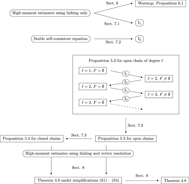
Figure 5.2: The structure of the proof of Theorem 4.8. Concepts and arguments are displayed in rounded boxes, statements and results in rectangular boxes.

We conclude this section with an outline of Sections 6 – 9. In Section 6 we present a simple high-moment estimate that only uses the process of linking (see Definition 3.10); more algebraically, the argument of Section 6 only uses Family A identities (and not Family B). The result is Proposition 6.1, which obtains a gain of a factor $\Psi$ from each $Q$ but no gain from charged vertices (see Definition 4.7). The goal of Section 6 is twofold, the first goal being pedagogical. It provides a complete but vastly simplified proof of a special case of Theorem 4.8, thereby illustrating the process of linking. In addition, it lays the ground for Step $\rm I_{1}$ used to derive a priori bounds on chains, as well as for the more complicated high-moment estimates used in the full proof of Theorem 4.8.

Section 6 is devoted to chains; its goal is to prove Proposition 5.3. Step $\rm I_{1}$ is proved in Section 7.1 and Step $\rm I_{2}$ in Section 7.2. The induction, and hence the proof of Proposition 5.3, is completed in Section 7.3. In Section 8 we prove Theorem 4.8 under four simplifying assumptions, (S1) – (S4) listed in Sections 6 and 8. These simplifications allow us to ignore some additional complications, and give a streamlined argument in which the fundamental mechanism is evident. The starting point for the argument in Section 8 is the high-moment expansion using vertex linking, already introduced in Section 6. In addition, we make use of Family B identities, which leads us to the process of vertex resolution (sketched in Section 3.2.4). In Section 9 we present the additional arguments needed to drop Simplifications (S1) – (S4), and hence prove Theorem 4.8 in full generality. Finally, in Section 10 we prove Theorem 4.15 as a relatively easy consequence of Theorem 4.8.

6 Warmup: simple high-moment estimates

We now move on to the high-moment estimates which underlie our proofs. The idea is to derive high-probability bounds on $X_{F}^{w}(\Delta)$ by controlling its high moments using a graphical expansion scheme.

For pedagogical reasons, we shall throughout the following selectively ignore some complications so as to make the core strategy clearer. We shall eventually put back the complications one by one. In this section we consistently assume the following simplification.

• All summation indices in the expanded summation $\mathbb{E}\lvert X_{F}^{w}(\Delta)\rvert^{p}$ (see (6.5) below) are distinct. (I.e. we ignore repeated indices which give rise to a smaller combinatorics of the summation.)

In this section we present a simple argument which proves the following weaker estimate.

Proposition 6.1.

Suppose that $\Lambda\prec\Psi$ for some admissible control parameter $\Psi$, $\Delta\in\mathfrak{Z}$, and $w$ is an adapted weight. Then for all $F\subset V_{s}(\Delta)$ and $\bm{\mathrm{\mu}}$ we have

$$X_{F}^{w}(\Delta)\;\prec\;\Psi^{\deg(\Delta)+\lvert F\rvert}\,.$$ (6.1)

The estimate (6.1) expresses that from each $Q$ in $X_{F}^{w}(\Delta)$ one gains an additional factor $\Psi$.

Remark 6.2.

As in Remark 4.12, the statement of Proposition 6.1 remains true if some (or all) diagonal entries of the form $\mathcal{G}_{aa}=G_{aa}-m$ are replaced by $1/G_{aa}-1/m$. The proof is exactly the same.

The simplified argument behind the proof of Proposition 6.1 uses only the Family A identities, i.e. (3.13). It relies on a high-moment estimate of the following form. The precise statement is somewhat complicated by the need to keep track of low-probability exceptional events. The sum over $\Gamma\in\mathfrak{G}$ in Lemma 6.3 will arise as a summation over graphs.

Lemma 6.3.

Suppose that $\Lambda\prec\Psi$ for some admissible control parameter $\Psi$, and let $p\in 2\mathbb{N}$ be even. Then we have

$$\mathbb{E}\lvert X_{F}^{w}(\Delta)\rvert^{p}\;\leqslant\;\sum_{\Gamma\in\mathfrak{G}}\mathbb{E}X_{\Gamma}\,,$$ (6.2)

where $\mathfrak{G}$ is a finite set (depending on $\Delta$, $F$, and $p$) and $X_{\Gamma}$ is a random variable satisfying

$$X_{\Gamma}\;\prec\;\Psi^{p(\deg(\Delta)+\lvert F\rvert)}$$ (6.3)

as well as the rough bound

$$\mathbb{E}\lvert X_{\Gamma}\rvert^{2}\;\leqslant\;N^{C_{p}}$$ (6.4)

for some constant $C_{p}$.

Before proving Lemma 6.3, we show how it implies Proposition 6.1.

Proof of Proposition 6.1.

Let $\varepsilon>0$ and $D>0$ be given. Define $p$ as the smallest even number greater than $4D/\varepsilon$, and abbreviate $q\mathrel{\vbox{\hbox{.}\hbox{.}}}=\deg(\Delta)+\lvert F\rvert$. Then by Lemma 6.3, for each $\Gamma\in\mathfrak{G}$ there exists an event $\Xi_{\Gamma}$ such that

$$\lvert X_{\Gamma}\rvert\bm{\mathrm{1}}(\Xi_{\Gamma})\;\leqslant\;N^{\varepsilon p/2}\Psi^{pq}\,,\qquad\mathbb{P}(\Xi_{\Gamma}^{c})\;\leqslant\;N^{-C_{p}-pq}$$

for all $w$, $\bm{\mathrm{\mu}}$, and $z\in\bm{\mathrm{S}}$. Then we find, using Lemma 6.3 again,

$$\mathbb{E}\lvert X_{F}^{w}(\Delta)\rvert^{p} \;\leqslant\;\sum_{\Gamma\in\mathfrak{G}}\Bigl{(}{\mathbb{E}\bigl{(}{X_{\Gamma}\bm{\mathrm{1}}(\Xi_{\Gamma})}\bigr{)}+\mathbb{E}\bigl{(}{X_{\Gamma}\bm{\mathrm{1}}(\Xi^{c}_{\Gamma})}\bigr{)}}\Bigr{)}$$

$$\;\leqslant\;\sum_{\Gamma\in\mathfrak{G}}\Bigl{(}{N^{\varepsilon p/2}\Psi^{pq}+\bigl{(}{\mathbb{E}\lvert X_{\Gamma}\rvert^{2}}\bigr{)}^{1/2}\mathbb{P}(\Xi_{\Gamma}^{c})^{1/2}}\Bigr{)}$$

$$\;\leqslant\;\bigl{\lvert}\mathfrak{G}\bigr{\rvert}\Bigl{(}{N^{\varepsilon p/2}\Psi^{pq}+N^{-pq/2}}\Bigr{)}$$

$$\;\leqslant\;2\bigl{\lvert}\mathfrak{G}\bigr{\rvert}N^{\varepsilon p/2}\Psi^{pq}\,,$$

for all $w$, $\bm{\mathrm{\mu}}$, and $z\in\bm{\mathrm{S}}$. Therefore Chebyshev’s inequality gives

$$\mathbb{P}\Bigl{(}{\lvert X_{F}^{w}(\Delta)\rvert>N^{\varepsilon}\Psi^{q}}\Bigr{)}\;\leqslant\;2\bigl{\lvert}\mathfrak{G}\bigr{\rvert}N^{-\varepsilon p/2}\;\leqslant\;N^{-D}$$

for all $w$, $\bm{\mathrm{\mu}}$, and $z\in\bm{\mathrm{S}}$. ∎

The rest of this section is devoted to the proof of Lemma 6.3. All of our estimates will be uniform in $w$ and $\bm{\mathrm{\mu}}$, and we shall henceforth no longer mention this explicitly. Throughout this section we assume Simplification (S1).

Proof of Lemma 6.3.

The idea of the proof was already outlined in Section 3.2.1. Let $\Delta\in\mathfrak{Z}$ have $n$ summation indices, denoted by $a_{1},\dots,a_{n}$, and $k$ external indices, denoted by $\mu_{1},\dots,\mu_{k}$. Let $F\subset\{1,\dots,n\}$. Let $p\in 2\mathbb{N}$ be even and write

$$\mathbb{E}\lvert X_{F}^{w}(\Delta)\rvert^{p}\;=\;\sum^{(\bm{\mathrm{\mu}})*}_{\bm{\mathrm{a}}^{1}}w(\bm{\mathrm{a}}^{1})\cdots\sum^{(\bm{\mathrm{\mu}})*}_{\bm{\mathrm{a}}^{p}}w(\bm{\mathrm{a}}^{p})\mathbb{E}\prod_{j=1}^{p/2}\Biggl{[}{\Biggl{(}{\prod_{i\in F}Q_{a_{i}^{j}}}\Biggr{)}\mathcal{Z}_{\bm{\mathrm{a}}^{j}}}\Biggr{]}\prod_{j=p/2+1}^{p}\overline{\Biggl{[}{\Biggl{(}{\prod_{i\in F}Q_{a_{i}^{j}}}\Biggr{)}\mathcal{Z}_{\bm{\mathrm{a}}^{j}}}\Biggr{]}}\!\,\,,$$ (6.5)

where we abbreviated

$$\bm{\mathrm{a}}^{j}\;\mathrel{\vbox{\hbox{.}\hbox{.}}}=\;({a^{j}_{i}\mathrel{\vbox{\hbox{.}\hbox{.}}}1\leqslant i\leqslant n})\,,\qquad\bm{\mathrm{a}}\;\mathrel{\vbox{\hbox{.}\hbox{.}}}=\;\bigl{(}{a_{i}^{j}\mathrel{\vbox{\hbox{.}\hbox{.}}}1\leqslant i\leqslant n\,,\,1\leqslant j\leqslant p}\bigr{)}\,.$$

We now make the crucial observation that $\widehat{w}(\bm{\mathrm{a}})\mathrel{\vbox{\hbox{.}\hbox{.}}}=w(\bm{\mathrm{a}}^{1})\ldots w(\bm{\mathrm{a}}^{j})$ is a weight on the set of indices $(i,j)$; this is an elementary consequence of the Definition (4.4). In particular, $\sum_{\bm{\mathrm{a}}}\widehat{w}(\bm{\mathrm{a}})\leqslant 1$.

By Simplification (S1), we assume that all indices $\bm{\mathrm{a}}$ are distinct: in addition to the constraint $a_{i}^{j}\notin\{\mu_{1},\dots,\mu_{k}\}$, we introduce into (6.5) an indicator function that imposes $a_{i}^{j}\neq a_{i^{\prime}}^{j^{\prime}}$ if $(i,j)\neq(i^{\prime},j^{\prime})$.

We now make each $\mathcal{G}_{xy}$ independent of as many summation indices as possible using Family A identities. To that end, we define

$$\mathcal{G}_{ij}^{(T)}\;\mathrel{\vbox{\hbox{.}\hbox{.}}}=\;G^{(T)}_{ij}-\delta_{ij}\,m\,.$$

Using (3.13) iteratively, we expand every factor $\mathcal{G}_{xy}$ appearing in (6.5) in all the indices

$$\bm{\mathrm{a}}_{F}\;\mathrel{\vbox{\hbox{.}\hbox{.}}}=\;\bigl{(}{a_{i}^{j}\mathrel{\vbox{\hbox{.}\hbox{.}}}i\in F\,,\,1\leqslant j\leqslant p}\bigr{)}$$

associated with a factor $Q$. Let $\mathcal{G}_{xy}$ be a fixed entry in (6.5). The idea is to successively add to $\mathcal{G}_{xy}$ as many upper indices from the collection $\bm{\mathrm{a}}_{F}$ as possible. The goal is to obtain a quantity satisfying the following definition.

Definition 6.4.

An entry $G_{xy}^{(T)}$ or $\mathcal{G}_{xy}^{(T)}$ is maximally expanded in $S$ if $S\subset T\sqcup\{x,y\}$. In other words, a maximally expanded resolvent entry cannot be expanded any further in the indices $S$ using (3.13).

Along the expansion of each $\mathcal{G}_{xy}$ using (3.13), new terms in (6.5) appear; each such term is a monomial of entries of $\mathcal{G}$ divided by diagonal entries of $G$. We stop expanding a term if either

• all its factors are maximally expanded in $\bm{\mathrm{a}}_{F}$, or

• it contains $\deg(\Delta)+2pn$ entries of $\mathcal{G}$ in the numerator.

The precise recursive procedure is as follows. We start by setting $A\mathrel{\vbox{\hbox{.}\hbox{.}}}=\mathcal{G}_{xy}$, where $\mathcal{G}_{xy}$ is an entry on the right-hand side of (6.5).

• Let $\mathcal{G}_{uv}^{(T)}$ denote an entry in $A$ and $d$ an index in $\bm{\mathrm{a}}_{F}$ such that $d\notin T\cup\{u,v\}$. (This choice is arbitrary and unimportant.) If (a) no such pair exists, or (b) $A$ contains $\deg(\Delta)+2pn$ factors $\mathcal{G}$ in the numerator, stop the recursion of the term $A$.

• Using Family A identities, write

  $$\mathcal{G}^{(T)}_{uv}\;=\;\mathcal{G}_{uv}^{(Td)}+\frac{\mathcal{G}_{ud}^{(T)}\mathcal{G}_{dv}^{(T)}}{G_{dd}^{(T)}}$$ (6.6)

  if $\mathcal{G}_{uv}^{(T)}$ is a resolvent entry in the numerator and

  $$\frac{1}{G_{uu}^{(T)}}\;=\;\frac{1}{G_{uu}^{(Td)}}-\frac{\mathcal{G}_{ud}^{(T)}\mathcal{G}_{du}^{(T)}}{G_{uu}^{(T)}G_{uu}^{(Td)}G_{dd}^{(T)}}$$ (6.7)

  if $G_{uv}^{(T)}=G_{uu}^{(T)}$ is a diagonal resolvent entry in the denominator. This yields the splitting $A=A^{\prime}+A^{\prime\prime}$, where both terms have the form of a product of entries in the numerator and diagonal entries in the denominator. Repeat step 1 for both $A^{\prime}$ and $A^{\prime\prime}$ (playing the role of $A$ in step 1).

It is not hard to see that the stopping rule defined by the conditions (a) or (b) ensures that the recursion terminates after a finite number of steps. Indeed, the quantity “number of entries of $\mathcal{G}$” + “number of upper indices” must remain bounded by the stopping rules (a) and (b).

The result is of the form

$$\mathcal{G}_{xy}\;=\;\sum_{\alpha}H_{\alpha}+R\,,$$

where each summand $H_{\alpha}$ is a fraction with entries of $\mathcal{G}$ in the numerator and diagonal entries of $G$ in the denominator, all of them maximally expanded in $\bm{\mathrm{a}}_{F}$. Here the rest term $R$ satisfies

$$R\;\prec\;\Psi^{\deg(\Delta)+2pn}\,,\qquad\mathbb{E}\lvert R\rvert^{2}\;\leqslant\;N^{C_{p,\Delta}}$$ (6.8)

for some constant $C_{p,\Delta}$. The first estimate of (6.8) follows from (3.16) combined with (3.11) and Lemma 3.6, and the second estimate of (6.8) from (3.18) and (3.19).

We then multiply the resulting sums on the right-hand side of (4.2) out to get

$$\mathcal{Z}_{\bm{\mathrm{a}}^{j}}\;=\;\sum_{\alpha}Y^{j,\alpha}_{\bm{\mathrm{a}}}\,,$$ (6.9)

where $Y^{j,\alpha}_{\bm{\mathrm{a}}}$ is a monomial and $\alpha$ a counting index ranging over some finite set. Each term $Y_{\bm{\mathrm{a}}}^{j,\alpha}$ is a fraction with entries of $\mathcal{G}$ in the numerator and diagonal entries of $F$ in the denominator. Moreover, either (i) all entries of $Y_{\bm{\mathrm{a}}}^{j,\alpha}$ are maximally expanded in $\bm{\mathrm{a}}_{F}$ or (ii) $Y_{\bm{\mathrm{a}}}^{j,\alpha}\prec\Psi^{\deg(\Delta)+2pn}$ (the latter arises if $Y_{\bm{\mathrm{a}}}^{j,\alpha}$ contains one or more rest terms $R$). We now multiply out the expectation in (6.5) as

$$\mathbb{E}\Biggl{[}{\Biggl{(}{\prod_{i\in F}Q_{a_{i}^{1}}}\Biggr{)}\mathcal{Z}_{\bm{\mathrm{a}}^{1}}}\Biggr{]}\cdots\Biggl{[}{\Biggl{(}{\prod_{i\in F}Q_{a_{i}^{p}}}\Biggr{)}\overline{\mathcal{Z}_{\bm{\mathrm{a}}^{p}}}\!\,}\Biggr{]}\;=\;\sum_{\alpha_{1},\dots,\alpha_{p}}\mathbb{E}\Biggl{[}{\Biggl{(}{\prod_{i\in F}Q_{a_{i}^{1}}}\Biggr{)}Y_{\bm{\mathrm{a}}}^{1,\alpha_{1}}}\Biggr{]}\cdots\Biggl{[}{\Biggl{(}{\prod_{i\in F}Q_{a_{i}^{p}}}\Biggr{)}\overline{Y_{\bm{\mathrm{a}}}^{p,\alpha_{p}}}\!\,}\Biggr{]}\,.$$ (6.10)

We plug this into (6.5) and pull out the summation over $\alpha_{1},\dots,\alpha_{p}$. This gives rise to the summation in (6.2), indexed by the set $\mathfrak{G}=\{(\alpha_{1},\dots,\alpha_{p})\}$. If, for some $(\alpha_{1},\dots,\alpha_{p})$, one or more of $Y^{1,\alpha_{1}}_{\bm{\mathrm{a}}},\dots,Y^{p,\alpha_{p}}_{\bm{\mathrm{a}}}$ is not maximally expanded in $\bm{\mathrm{a}}_{F}$, it is easy to see that

$$X_{\alpha_{1}\cdots\alpha_{p}}\;\mathrel{\vbox{\hbox{.}\hbox{.}}}=\;\sum^{(\bm{\mathrm{\mu}})*}_{\bm{\mathrm{a}}^{1}}w(\bm{\mathrm{a}}^{1})\cdots\sum^{(\bm{\mathrm{\mu}})*}_{\bm{\mathrm{a}}^{p}}w(\bm{\mathrm{a}}^{p})\Biggl{[}{\Biggl{(}{\prod_{i\in F}Q_{a_{i}^{1}}}\Biggr{)}Y_{\bm{\mathrm{a}}}^{1,\alpha_{1}}}\Biggr{]}\cdots\Biggl{[}{\Biggl{(}{\prod_{i\in F}Q_{a_{i}^{p}}}\Biggr{)}\overline{Y_{\bm{\mathrm{a}}}^{p,\alpha_{p}}}\!\,}\Biggr{]}$$ (6.11)

satisfies (6.3) and (6.4). Indeed, each term $Y_{\bm{\mathrm{a}}}^{j,\alpha_{j}}$ contains at least $\deg(\Delta)$ entries of $\mathcal{G}$; thus the trivial bound $Y_{\bm{\mathrm{a}}}^{j,\alpha_{j}}\prec\Psi^{\deg(\Delta)}$ always holds by Lemma 3.9. Using Lemma 3.6 we can multiply these estimates. Recalling (6.8), (3.18), and (3.19), we find (6.3) and (6.4).

It therefore suffices to consider products of $Y_{\bm{\mathrm{a}}}^{j,\alpha_{j}}$’s in (6.10) which are all maximally expanded in $\bm{\mathrm{a}}_{F}$ (i.e. terms which are products of $H_{\alpha}$’s only and not $R$’s). The presence of $Q$’s leads to the following crucial restriction on terms yielding a nonzero contribution to (6.10). For each $i\in F$, we claim that at least one of $Y_{\bm{\mathrm{a}}}^{2,\alpha_{2}},\dots,Y_{\bm{\mathrm{a}}}^{p,\alpha_{p}}$ is not independent of $a_{i}^{1}$. This follows from the observation that generally $\mathbb{E}[Q_{a}(X)Y]=0$ if $Y$ is independent of $a$. More generally, we require that, for any $i\in F$ and $j=1,\dots,p$, at least of one of

$$Y_{\bm{\mathrm{a}}}^{1,\alpha_{1}},\dots,\widehat{Y_{\bm{\mathrm{a}}}^{j,\alpha_{j}}},\dots,Y_{\bm{\mathrm{a}}}^{p,\alpha_{p}}$$

is not independent of $a_{i}^{j}$ (hat indicates omission from the list). This imposes a constraint on the terms that survive the expansion.

Moreover, the term that is not independent of $a_{i}^{j}$ contains at least one additional entry of $\mathcal{G}$, since at some point the formula (6.6) or (6.7) had to be applied with $d=a_{i}^{j}$ and the second term of (6.6) or (6.7) contains at least one additional entry of $\mathcal{G}$. Since we assumed Simplification (S1), i.e. all $a_{i}^{j}$’s are different, it is a general fact that each $Q$ gives rise to an additional off-diagonal entry of $\mathcal{G}$ and contributes a factor $\Lambda\prec\Psi$ to (6.5). In other words, any $X_{\alpha_{1}\cdots\alpha_{p}}$ yielding a nonzero contribution to (6.5) has at least $p(\deg(\Delta)+\lvert F\rvert)$ entries of $\mathcal{G}$ in the numerator. Recalling Lemma 3.6 and Lemma 3.9, we find that any term $X_{\alpha_{1}\cdots\alpha_{p}}$ yielding a nonzero contribution to (6.5) satisfies (6.3) and (6.4). This concludes the proof of Lemma 6.3. ∎

6.1.  Graphical representation

The phenomenon behind the proof of Lemma 6.3 in fact has a simple graphical representation, which will prove essential for later, more intricate, estimates. We illustrate its usefulness by applying it to the proof of Lemma 6.3. We recall the basic graphical notation introduced in Section 3.2.2.

The quantity whose expectation we are estimating, $\lvert X_{F}^{w}(\Delta)\rvert^{p}=\big{[}X_{F}^{w}(\Delta)\big{]}^{p/2}\big{[}\overline{X_{F}^{w}(\Delta)}\big{]}^{p/2}$, has a natural representation in terms of a multigraph, which we call $\gamma^{p}(\Delta)$ and which is essentially a $p$-fold copy of the graph $\Delta$ encoding $\mathcal{Z}$. The graph $\gamma^{p}(\Delta)$ is obtained as follows.

1. Take $p/2$ copies of $\Delta$ and $p/2$ copies of $\Delta$ whose edges have inverted direction and colour arising from the relation $\overline{\mathcal{G}}_{ab}=\mathcal{G}_{ba}^{*}$. More precisely, this inversion means that each edge $e\in E(\Delta)$ gives rise to an inverted edge $e^{\prime}$ satisfying

   $$\xi_{e^{\prime}}\;=\;\begin{cases}1&\text{if }\xi_{e}=*\\ *&\text{if }\xi_{e}=1\,,\end{cases}\qquad\alpha(e^{\prime})\;=\;\beta(e)\,,\qquad\beta(e^{\prime})\;=\;\alpha(e)\,.$$

2. For each external vertex $i\in V_{e}(\Delta)$ merge all $p$ copies of $i$ to form a single vertex.

Note that the set $F$ is not depicted in $\gamma^{p}(\Delta)$. The vertex set of $\gamma^{p}(\Delta)$ consists of summation vertices and external vertices (this classification is inherited from the vertices of $\Delta$ in the obvious way), so that we may write $V(\gamma^{p}(\Delta))=V_{s}(\gamma^{p}(\Delta))\sqcup V_{e}(\gamma^{p}(\Delta))$.

Definition 6.5 (Projection $\pi$).

We introduce the $p$-to-one canonical projection $\pi\mathrel{\vbox{\hbox{.}\hbox{.}}}V(\gamma^{p}(\Delta))\to V(\Delta)$, defined as $\pi(i)=j$ if $i$ is a copy of $j$ in the construction of $\gamma^{p}(\Delta)$.

Figure 6.1: The graph $\gamma^{2}(\Delta)$ that encodes $\mathbb{E}\lvert X_{F}^{w}(\Delta)\rvert^{2}$, where $\mathcal{Z}_{a_{1}a_{2}}\;=\;\mathcal{G}_{\mu_{1}a_{1}}\mathcal{G}_{a_{1}a_{2}}\mathcal{G}_{a_{2}\mu_{2}}^{*}\mathcal{G}_{a_{1}a_{2}}^{*}\mathcal{G}_{\mu_{2}a_{1}}$.

We start with the graph $\gamma^{p}(\Delta)$ (see Figure 6.1). We shall construct a set $\widetilde{\mathfrak{G}}_{F}^{p}(\Delta)$ of graphs, denoted by $\Gamma$, on the same vertex set $V(\gamma^{p}(\Delta))$. The algorithm that generates $\widetilde{\mathfrak{G}}_{F}^{p}(\Delta)$ is precisely the one given after Definition 6.4. On the level of graphs, this algorithm consists of a repeated application of the graphical rules in Figures 3.5 and 3.6. (Note that the second identity of Figure 3.6 is also valid for $\mathcal{G}$ instead of $G$, i.e. without the black diamonds.) As indicated in Figures 3.5 and 3.6, we keep track of the upper indices associated with an edge by attaching a list of upper indices to each edge. The algorithm terminates when either all edges are maximally expanded in $\bm{\mathrm{a}}_{F}$ or there are $\deg(\Delta)+pn$ edges that do not bear a diamond (i.e. that contribute a factor $\Psi$). Indicating these upper indices may be more precisely implemented using decorated edges, but we shall not need such formal constructions.

Recall from Definition 3.10 that choosing the second graph on the right-hand side of any identity in Figures 3.5 and 3.6 is called linking (an edge with a vertex). As shown above, any graph $\Gamma\in\widetilde{\mathfrak{G}}_{F}^{p}(\Delta)$ whose edges are not maximally expanded yields a small enough contribution by a trivial power counting. In the following we shall therefore only consider the remaining graphs, i.e. we shall assume that all edges of $\Gamma\in\widetilde{\mathfrak{G}}_{F}^{p}(\Delta)$ are maximally expanded in $\bm{\mathrm{a}}_{F}$. Moreover, the upper indices of an edge are uniquely determined by the constraint that the edge be maximally expanded: the entry encoded by the edge $(x,y)$ is $\mathcal{G}_{xy}^{(\bm{\mathrm{a}}_{F}\setminus\{x,y\})}$. Thus, we shall consistently drop the upper indices associated with edges from our graphs $\Gamma$.

We introduce some convenient notions when dealing with graphs in $\widetilde{\mathfrak{G}}_{F}^{p}(\Delta)$.

Definition 6.6.

Let $\Gamma\in\widetilde{\mathfrak{G}}_{F}^{p}(\Delta)$.

1. We denote the vertex set of $\Gamma$ by $V(\Gamma)=V_{s}(\Gamma)\sqcup V_{e}(\Gamma)$, where $V_{s}(\Gamma)$ denotes the summation vertices and $V_{e}(\Gamma)$ external (fixed) vertices. By definition, all three sets are the same as those of $\gamma^{p}(\Delta)$.

2. We denote the set of edges of $\Gamma$ by $E(\Gamma)$; the set $E(\Gamma)$ has a colouring $\xi\mathrel{\vbox{\hbox{.}\hbox{.}}}E(\Gamma)\to\{1,*\}$.

3. The $p$-to-one canonical projection $\pi\mathrel{\vbox{\hbox{.}\hbox{.}}}V(\Gamma)\to V(\Delta)$ is taken over from Definition 6.5.

Thus, $\bm{\mathrm{a}}_{F}=\bigl{(}{a_{i}\mathrel{\vbox{\hbox{.}\hbox{.}}}i\in\pi^{-1}(F)}\bigr{)}$. In this manner we write the sum of maximally expanded terms on the right-hand side of (6.10) as a sum of graphs $\Gamma\in\widetilde{\mathfrak{G}}^{p}_{F}(\Delta)$. By definition, each vertex in $\pi^{-1}(F)$ has been linked with at least one edge, possibly more. Each such linking adds an edge to the graph, and hence contributes a factor $\Lambda\prec\Psi$ to its size. This concludes the graphical discussion behind the proof of (6.1). Figure 6.2 shows two sample graphs from $\widetilde{\mathfrak{G}}_{F}^{2}(\Delta)$ for the graph $\Delta$ from Figure 6.1, where $F$ consists of a single vertex associated with the summation variable $a_{1}$.

Figure 6.2: Left: a graph obtained from the one in Figure 6.1 with $|F|=1$ by linking both vertices in $\bm{\mathrm{a}}_{F}=(a_{1}^{1},a_{1}^{2})$ with an edge; $a_{1}^{1}$ was linked with the edge $(\mu_{2},a_{2}^{2})$ and $a_{1}^{2}$ was linked with $(\mu_{1},a_{1}^{1})$. This graph contains the minimal number of edges to yield a nonzero contribution after taking the expectation. Hence it is of leading order. Right: a graph obtained by linking two further edges with $a_{1}^{1}$, namely the edges $(a_{1}^{2},\mu_{2})$ and $(\mu_{1},a_{1}^{2})$. Its size is subleading.

7 Chains

In this section we derive the a priori estimate on chains, Proposition 5.3.

7.1.  Step $\mathrm{I}_{1}$: chains with $F\neq\emptyset$

Step $\rm I_{1}$ is an application of the simple high-moment expansion method from Section 6. It is formulated in the following proposition. In Section 7.3, it will be used in conjunction with Proposition 7.2 below to complete the induction and hence the proof of Proposition 5.3.

Proposition 7.1 (Induction Step $\rm I_{1}$).

Suppose that $\Lambda\prec\Psi$ for some admissible control parameter $\Psi$, and let $\ell\geqslant 2$. Suppose that

$$X^{w}_{F}(\Delta)\;\prec\;\Psi^{\deg(\Delta)+\lvert F\rvert}\Phi^{c(\Delta)-\lvert F\rvert}$$ (7.1)

holds for any open chain $\Delta$ of degree strictly less than $\ell$, $F=\emptyset$, and any adapted chain weight $w$. Then (7.1) holds for any open chain $\Delta$ of degree $\ell$, $F\neq\emptyset$, and any adapted chain weight $w$.

In this section we continue to assume Simplification (S1) (see the beginning of Section 6).

Proof of Proposition 7.1.

For simplicity of notation, we focus on the case where $\Delta$ is a directed chain of degree $\ell$; the undirected case is proved in the same way. The argument is best understood in a representative example,

$$\mathcal{Z}_{\bm{\mathrm{a}}}\;=\;G_{\mu_{1}a_{1}}G_{a_{1}a_{2}}G_{a_{2}a_{3}}G_{a_{3}a_{4}}G_{a_{4}\mu_{2}}\,,$$ (7.2)

which is encoded by the graph $\Delta$ depicted in Figure 7.1.

Figure 7.1: The graph $\Delta$ that encodes $\mathcal{Z}$ defined in (7.2).

Let us take $F=\{1\}$ and compute the variance of $X_{F}^{w}(\Delta)$. In the following we use the terminology and notation of Section 6 without further comment. In Section 6 is was shown that the only graphs $\Gamma\in\widetilde{\mathfrak{G}}^{2}_{F}(\Delta)$ that contribute are those in which the vertices $a_{1}^{1}$ and $a_{1}^{2}$ have both been linked to some edge.

Figure 7.2: Left: a graph $\Gamma$ of leading order in $\widetilde{\mathfrak{G}}_{F}^{2}(\Delta)$ with $\Delta$ defined through (7.2), and $F=\{1\}$. We do not draw the loops that encode diagonal resolvent entries in the denominator. Right: the same graph broken down to chains.

Figure 7.2 shows such a graph $\Gamma$ of leading order. Since the two vertices $a_{1}^{1}$ and $a_{1}^{2}$ have been linked, they each contribute a factor $\Lambda\prec\Psi$ (two edges were added by the linking process). Now we break the graph in Figure 7.2 down to its chains, i.e. we freeze all those summation vertices, $a_{1}^{1}$ and $a_{1}^{2}$, that were linked to. What remains is a collection of chains, each shorter than the original chain $\Delta$. In this example there are four nontrivial subchains:

$$a_{1}^{1}\to a_{2}^{1}\to a_{3}^{1}\to a_{1}^{2}\,,\qquad a_{1}^{2}\to a_{4}^{1}\to\mu_{2}\,,\qquad\mu_{2}\to a_{4}^{2}\to a_{3}^{2}\to a_{1}^{1}\,,\qquad a_{1}^{1}\to a_{2}^{2}\to a_{1}^{2}\,.$$

Moreover, the monomial encoded by each subchain lies either inside $Q_{a_{1}^{1}}(\cdot)$, inside $Q_{a_{1}^{2}}(\cdot)$, or inside neither. Thus the monomials encoded by the first two subchains lie inside $Q_{a_{1}^{1}}(\cdot)$, and the monomials encoded by the two last subchains inside $Q_{a_{1}^{2}}(\cdot)$.

Now we may invoke the induction assumption (i.e. Proposition 5.3 for $F=\emptyset$) on each of the four subchains. We use that they all have degree strictly less than $\deg(\Delta)$. To be precise, before invoking Proposition 5.3, we have to get rid of the upper indices using (3.13); see below for details.

Moreover, we ignore some minor technicalities associated with coinciding indices. By Simplification (S1), we assumed that all summation indices of $\Gamma$ were distinct. In particular, the indices associated with different subchains of $\Gamma$ are distinct, which implies that the subchains of $\Gamma$ are coupled. This coupling is manifested in the fact that summation indices within a subchain are subject to additional restrictions that are unrelated to that subchain: these summation indices cannot take on values of indices in other subchains. This means that summations cannot be performed independently within each subchain. Hence we may not strictly speaking invoke Proposition 5.3 for each subchain; in order to do so, we first have to decouple the subchains so as to get a product of terms associated with the subchains. In order to achieve this decoupling we have to allow indices associated with different subchains to coincide. This decoupling is a simple inclusion-exclusion argument whose details are postponed to Lemma 9.5 in Section 9.3.

Summarizing this example, we obtain an estimate of order $\Psi^{12}\Phi^{6}$ for the graph depicted in Figure 7.2. Since, by Proposition 5.3, the contribution of an open subchain of degree $d$ is $\Psi^{d}\Phi^{d-1}$, the four non-trivial subchains yield a contribution $\Psi^{3}\Phi^{2}\,\Psi^{2}\Phi\,\Psi^{3}\Phi^{2}\,\Psi^{3}\Phi=\Psi^{10}\Phi^{6}$. There are also two trivial subchains, thus resulting in a total contribution $\Psi^{12}\Phi^{6}$. Another way to think about such estimates is to count the additional factors of $\Psi$ and $\Phi$ gained along the proof. The naive size of the original graph, before linking, was $\Psi^{2\deg(\Delta)}=\Psi^{10}$ since $\mathcal{Z}$ in (7.2) contains five factors and we consider its second moment (i.e. set $p=2$). Since $\lvert F\rvert=1$, we gain an additional $\Psi^{2\lvert F\rvert}=\Psi^{2}$ from the linking; this step increases the number of edges from 10 to 12 in the graph on the left-hand side of Figure 7.2. Moreover, we gain an additional $\Phi$ factor from each internal summation vertex in the subchains, in this example we gain a factor $\Phi$ from each of the six vertices $a_{2}^{1}$, $a_{3}^{1}$, $a_{4}^{1}$, $a_{4}^{2}$, $a_{3}^{2}$, and $a_{2}^{2}$. Thus we recover the bound $\Psi^{12}\Phi^{6}$.

Let us now give the general argument, which is in fact a trivial generalization of the above example. We start with a graph $\Gamma\in\widetilde{\mathfrak{G}}_{F}^{p}(\Delta)$, as constructed in Section 6. We split the summation indices $\bm{\mathrm{a}}=(\bm{\mathrm{a}}^{\prime},\bm{\mathrm{a}}^{\prime\prime})$, where $\bm{\mathrm{a}}^{\prime}$ consists of the chain vertices of $\Gamma$. Thus, $\bm{\mathrm{a}}^{\prime\prime}$ contains in particular the indices associated with vertices which have been linked to an edge. By the argument of Section 6, $\bm{\mathrm{a}}^{\prime\prime}$ contains all indices of $\bm{\mathrm{a}}_{F}$, so that $\lvert\bm{\mathrm{a}}^{\prime\prime}\rvert\geqslant\lvert\bm{\mathrm{a}}_{F}\rvert=p\lvert F\rvert$. Since each linked vertex is incident to an additional edge resulting from linking, the graph $\Gamma$ contains at least $p\deg(\Delta)+\lvert\bm{\mathrm{a}}_{F}\rvert\geqslant p(\deg(\Delta)+|F|)$ edges. So far we have simply repeated the argument of Section 6 and reproved the bound (6.1).

In order to gain an additional factor $\Phi$ from each of the summation indices in $\bm{\mathrm{a}}^{\prime}$, we use the induction assumption. The assumption is used on open chains of vertices, i.e. subgraphs of $\Gamma$ which are open chains. We fix $\bm{\mathrm{a}}^{\prime\prime}$ and regard $\bm{\mathrm{a}}^{\prime}$ as the summation indices. Then $\Gamma$ becomes a collection of open (sub)chains, and the vertices associated with $\bm{\mathrm{a}}^{\prime}$ are the chain vertices of these subchains. If we can ensure that each subchain has degree strictly less than $\Delta$, we can apply the induction assumption to get an additional factor $\Phi$ from each chain vertex in represented in $\bm{\mathrm{a}}^{\prime}$. This will give us a bound of size

$$\Psi^{p\deg(\Delta)+\lvert\bm{\mathrm{a}}^{\prime\prime}\rvert}\Phi^{\lvert\bm{\mathrm{a}}^{\prime}\rvert}\;\leqslant\;\Psi^{p(\deg(\Delta)+\lvert F\rvert)}\Phi^{p(c(\Delta)-\lvert F\rvert)}\,,$$

where we used that $\lvert\bm{\mathrm{a}}^{\prime\prime}\rvert\geqslant p\lvert F\rvert$, $\lvert\bm{\mathrm{a}}^{\prime\prime}\rvert+\lvert\bm{\mathrm{a}}^{\prime}\rvert=p\,c(\Delta)$, and $\Psi\leqslant\Phi$.

In order to carry out this argument, we make the following observations.

1. All subchains of $\Gamma$ have degree strictly less than $\deg(\Delta)$. This property is crucial for the induction. It is a consequence of the two following facts. First, the linking of vertices never produces new subchains nor lengthens pre-existing subchains. Note that vertices in $\bm{\mathrm{a}}^{\prime\prime}$ are fixed, and subchains terminate at them. Second, since $F\neq\emptyset$, at least one vertex of every subchain of degree $\deg(\Delta)$ in $\gamma^{p}(\Delta)$ will be linked to an edge, hence cutting the subchain of degree $\deg(\Delta)$ into smaller subchains.

2. The expression $\mathcal{Z}^{\prime}_{\bm{\mathrm{b}}}$ encoded by any subchain $\Gamma^{\prime}$ of $\Gamma$ always appears in conjunction with a chain weight $w^{\prime}(\bm{\mathrm{b}})$. This is an immediate consequence of the fact that the weight $w(\bm{\mathrm{a}}^{1})\cdots w(\bm{\mathrm{a}}^{p})$ is a chain weight by assumption.

3. Let $\mathcal{Z}^{\prime}_{\bm{\mathrm{b}}}$ denote the monomial encoded by a subchain $\Gamma^{\prime}$ of $\Gamma$. Then any $Q_{a}$ has an index $a$ in $\bm{\mathrm{a}}^{\prime\prime}$ (i.e. is fixed), and acts either on all resolvent entries of $\mathcal{Z}^{\prime}_{\bm{\mathrm{b}}}$ or none of them.

In order to invoke the induction assumption, we still have to get rid of the upper indices in the maximally expanded resolvent entries. The procedure is almost identical to the one following Definition 6.4, but in the opposite direction. In particular, the key formula (3.13) should be viewed in the form

$$G_{ij}^{(Tk)}\;=\;G_{ij}^{(T)}-\frac{G_{ik}^{(T)}G_{kj}^{(T)}}{G_{kk}^{(T)}}\,,\qquad\frac{1}{G_{ii}^{(Tk)}}\;=\;\frac{1}{G_{ii}^{(T)}}+\frac{G_{ik}^{(T)}G_{ki}^{(T)}}{G_{ii}^{(T)}G_{ii}^{(Tk)}G_{kk}^{(T)}}\,.$$ (7.3)

We start removing the upper indices one by one using (7.3), and stop if either all upper indices have been removed or if the number of off-diagonal resolvent entries exceeds $\deg(\Delta)+2p\ell$. The size of the latter terms is already sufficiently small by the trivial bound $\Lambda\prec\Psi$. As for the former terms, they are represented by a new (but still finite) set of graphs in which every vertex is either a chain vertex or has been linked with an edge.

Now the induction assumption is applicable to each subchain, and the proof is completed by invoking Lemma 3.6. (Note that as before we ignored issues related to coinciding indices according to Simplification (S1); these are dealt with using the inclusion-exclusion argument of Lemma 9.5.) ∎

7.2.  Step $\mathrm{I}_{2}$: chains with $F=\emptyset$

Step $\mathrm{I}_{2}$ is completed in the following proposition.

Proposition 7.2 (Induction Step $\mathrm{I}_{2}$).

Suppose that $\Lambda\prec\Psi$ for some admissible control parameter $\Psi$, and let $\ell\geqslant 2$. Suppose that

$$X^{w}_{F}(\Delta)\;\prec\;\Psi^{\deg(\Delta)+\lvert F\rvert}\Phi^{c(\Delta)-\lvert F\rvert}$$ (7.4)

holds for any open chain $\Delta$ of degree $\ell$, any $F\neq\emptyset$, and any adapted chain weight $w$. If $\ell\geqslant 3$, suppose in addition that (7.4) holds for any open chain $\Delta$ of degree strictly less than $\ell$, $F=\emptyset$, and any adapted chain weight $w$.

Then (7.4) holds for any open chain $\Delta$ of degree $\ell$, $F=\emptyset$, and any adapted chain weight $w$.

Proof.

As before, we focus on the case where $\Delta$ is a directed open chain; the proof in in the undirected case is the same. Thus,

$$\mathcal{Z}_{a_{1}\cdots a_{n}}\;=\;G_{\mu_{1}a_{1}}G_{a_{1}a_{2}}\cdots G_{a_{n}\mu_{2}}\,,\qquad w_{\bm{\mathrm{b}}}(\bm{\mathrm{a}})\;\equiv\;w(\bm{\mathrm{a}})\;=\;s_{a_{1}b_{1}}\cdots s_{a_{n}b_{n}}$$

for some $\bm{\mathrm{b}}=\{b_{1},\dots,b_{n}\}$. (Recall that $G_{ij}=\mathcal{G}_{ij}$ for $i\neq j$.) Note that $n=\deg(\Delta)-1$. We have to prove that

$$X_{\emptyset}^{w}(\Delta)\;\prec\;\Psi^{n+1}\Phi^{n}\,.$$ (7.5)

(Here we used that $c(\Delta)=n$.) The main idea of the proof was given in Section 3.2.3: derive a stable self-consistent equation whose error terms may be estimated using the induction assumption. We subdivide the proof into six steps.

To simplify notation, throughout this proof we use $\mathcal{E}\equiv\mathcal{E}(\bm{\mathrm{b}},\mu_{1},\mu_{2})$ to denote a random error term satisfying $\mathcal{E}\prec\Psi^{n+2}\Phi^{n-1}$. Like generic constants $C$, these error terms may change from line to line without changing name.

Moreover, in order to keep the presentation more concise, we shall sometimes ignore unimportant subtleties arising from coinciding summation indices. These complications are harmless and will be dealt with precisely using the inclusion-exclusion argument of Lemma 9.5. The general philosophy is the following: if we constrain a pair of indices to coincide instead of being distinct, we lose at most two factors of $\Psi$. Indeed, we lose at most one chain vertex (resulting in a loss of $\Phi\geqslant\Psi$), and at most one off-diagonal entry of $G$ may become diagonal (resulting in a loss of $\Psi$). Note that, since $\Delta$ is an open chain, at most one off-diagonal entry may become diagonal when setting two summation indices to be equal. (This is not true for closed chains; see Section 7.3.) This loss of $\Psi^{2}$ is compensated by the factor $M^{-1}\leqslant\Psi^{2}$ we gain from the reduction in the number of summation variables.

Step (i). We introduce a factor $P_{a_{1}}$ into the summation in $X_{\emptyset}^{w}(\Delta)$. We find

$$X_{\emptyset}^{w}(\Delta) \;=\;\sum_{\bm{\mathrm{a}}}^{(\mu_{1}\mu_{2})*}w(\bm{\mathrm{a}})\,P_{a_{1}}\mathcal{Z}_{a_{1}\cdots a_{n}}+X_{\{1\}}^{w}(\Delta)$$

$$\;=\;\sum_{\bm{\mathrm{a}}}^{(\mu_{1}\mu_{2})*}w(\bm{\mathrm{a}})\,P_{a_{1}}\mathcal{Z}_{a_{1}\cdots a_{n}}+\mathcal{E}\,.$$

where the second equality follows from the induction assumption.

Step (ii). We introduce a factor $m^{2}/(G_{a_{1}a_{1}})^{2}$ in front of $X_{\emptyset}^{w}(\Delta)$; this prefactor will be important in the fourth step below, as the factor $1/(G_{a_{1}a_{1}})^{2}$ will be used to cancel diagonal resolvent entries arising from two applications of the identity (3.14a). We find

$$\sum_{\bm{\mathrm{a}}}^{(\mu_{1}\mu_{2})*}w(\bm{\mathrm{a}})\,P_{a_{1}}\mathcal{Z}_{a_{1}\cdots a_{n}} \;=\;\sum_{\bm{\mathrm{a}}}^{(\mu_{1}\mu_{2})*}w(\bm{\mathrm{a}})P_{a_{1}}\Biggl{[}{\frac{(G_{a_{1}a_{1}}-m)^{2}+2m(G_{a_{1}a_{1}}-m)+m^{2}}{(G_{a_{1}a_{1}})^{2}}\mathcal{Z}_{a_{1}\cdots a_{n}}}\Biggr{]}$$

$$\;=\;\sum_{a_{1}}^{(\mu_{1}\mu_{2})}s_{a_{1}b_{1}}P_{a_{1}}\Biggl{[}G_{\mu_{1}a_{1}}\frac{(G_{a_{1}a_{1}}-m)^{2}+2m(G_{a_{1}a_{1}}-m)+m^{2}}{(G_{a_{1}a_{1}})^{2}}$$

$$\mspace{40.0mu}\times\sum_{a_{2},\dots,a_{n}}^{(a_{1}\mu_{1}\mu_{2})*}s_{a_{2}b_{2}}\cdots s_{a_{n}b_{n}}G_{a_{1}a_{2}}\cdots G_{a_{n}\mu_{2}}\Biggr{]}\,.$$

For $n=1$ (i.e. $\deg(\Delta)=2$) the last line is understood to be $G_{a_{1}\mu_{2}}$.

We now show that the only the term $m^{2}$ in the numerator is relevant. By induction assumption and Lemma 3.6, we find that

$$\sum_{a_{2},\dots,a_{n}}^{(a_{1}\mu_{1}\mu_{2})*}s_{a_{2}b_{2}}\cdots s_{a_{n}b_{n}}G_{a_{1}a_{2}}\cdots G_{a_{n}\mu_{2}}\;\prec\;\Psi^{n}\Phi^{n-1}\,.$$ (7.6)

(Note that the induction assumption is only used if $n\geqslant 2$; for the initial value $n=1$ (7.6) is trivial.) Using $\sum_{a_{1}}s_{a_{1}b_{1}}\leqslant 1$, (3.17), and Lemma 3.6 again, we get

$$X_{\emptyset}^{w}(\Delta)\;=\;\widetilde{X}_{\emptyset}^{w}(\Delta)+\mathcal{E}\,,\qquad\widetilde{X}_{\emptyset}^{w}(\Delta)\;\mathrel{\vbox{\hbox{.}\hbox{.}}}=\;\sum_{\bm{\mathrm{a}}}^{(\mu_{1}\mu_{2})*}w(\bm{\mathrm{a}})\,P_{a_{1}}\biggl{[}{\frac{m^{2}}{(G_{a_{1}a_{1}})^{2}}\mathcal{Z}_{a_{1}\cdots a_{n}}}\biggr{]}\,.$$ (7.7)

Step (iii). We make all resolvent entries which do not contain the index $a_{1}$ independent of $a_{1}$ using (3.13). Thus, we assume that $n\geqslant 2$; if $n=1$ there is nothing to be done and this step is trivial. Using (3.13) we find

$$\widetilde{X}_{\emptyset}^{w}(\Delta) \;=\;\sum_{\bm{\mathrm{a}}}^{(\mu_{1}\mu_{2})*}w(\bm{\mathrm{a}})\,P_{a_{1}}\biggl{[}{\frac{m^{2}}{(G_{a_{1}a_{1}})^{2}}G_{\mu_{1}a_{1}}G_{a_{1}a_{2}}G_{a_{2}a_{3}}G_{a_{3}a_{4}}\cdots G_{a_{n}\mu_{2}}}\biggr{]}$$

$$\;=\;\sum_{\bm{\mathrm{a}}}^{(\mu_{1}\mu_{2})*}w(\bm{\mathrm{a}})\,P_{a_{1}}\biggl{[}{\frac{m^{2}}{(G_{a_{1}a_{1}})^{2}}G_{\mu_{1}a_{1}}G_{a_{1}a_{2}}\biggl{(}{G_{a_{2}a_{3}}^{(a_{1})}+\frac{G_{a_{2}a_{1}}G_{a_{1}a_{3}}}{G_{a_{1}a_{1}}}}\biggr{)}G_{a_{3}a_{4}}\cdots G_{a_{n}\mu_{2}}}\biggr{]}$$

$$\;=\;\sum_{\bm{\mathrm{a}}}^{(\mu_{1}\mu_{2})*}w(\bm{\mathrm{a}})\,P_{a_{1}}\biggl{[}{\frac{m^{2}}{(G_{a_{1}a_{1}})^{2}}G_{\mu_{1}a_{1}}G_{a_{1}a_{2}}G_{a_{2}a_{3}}^{(a_{1})}G_{a_{3}a_{4}}\cdots G_{a_{n}\mu_{2}}}\biggr{]}+\mathcal{E}\,.$$

Here the bound on the error term

$$\sum_{a_{1}}^{(\mu_{1}\mu_{2})}s_{a_{1}b_{1}}P_{a_{1}}\Biggl{[}{\frac{m^{2}}{(G_{a_{1}a_{1}})^{3}}G_{\mu_{1}a_{1}}\sum_{a_{2},\dots,a_{n}}^{(a_{1}\mu_{1}\mu_{2})*}s_{a_{2}b_{2}}\cdots s_{a_{n}b_{n}}\,G_{a_{1}a_{2}}G_{a_{2}a_{1}}G_{a_{1}a_{3}}G_{a_{3}a_{4}}\cdots G_{a_{n}\mu_{2}}}\Biggr{]}$$

follows by first fixing the summation index $a_{1}$ and using the induction assumption combined with Lemma 3.6, similarly to Step (ii) above. The induction assumption is used on two chains: one of degree $2$ (corresponding to $G_{a_{1}a_{2}}G_{a_{2}a_{1}}$) and one of degree $n-1$ (corresponding to $G_{a_{1}a_{3}}G_{a_{3}a_{4}}\cdots G_{a_{n}\mu_{2}}$); here $a_{1}$ is regarded as an external index. (Here we swept under the rug a minor technicality. Strictly speaking, the expressions encoded by different subchains do not factor, since their summations are still coupled by the constraint $a_{2}\notin\{a_{1},a_{3},a_{4},\dots,a_{n}\}$. As outlined above, we ignore such complications here; they are dealt with using the inclusion-exclusion argument from Lemma 9.5 in Section 9.3 by introducing a partitioning on the values of $a_{2}$, which results in a decoupled expression plus a series of small error terms.)

Next, we write

$$\sum_{\bm{\mathrm{a}}}^{(\mu_{1}\mu_{2})*}w(\bm{\mathrm{a}})\,P_{a_{1}}\biggl{[}{\frac{m^{2}}{(G_{a_{1}a_{1}})^{2}}G_{\mu_{1}a_{1}}G_{a_{1}a_{2}}G_{a_{2}a_{3}}^{(a_{1})}G_{a_{3}a_{4}}G_{a_{4}a_{5}}\cdots G_{a_{n}\mu_{2}}}\biggr{]}\\ =\;\sum_{\bm{\mathrm{a}}}^{(\mu_{1}\mu_{2})*}w(\bm{\mathrm{a}})\,P_{a_{1}}\biggl{[}{\frac{m^{2}}{(G_{a_{1}a_{1}})^{2}}G_{\mu_{1}a_{1}}G_{a_{1}a_{2}}G_{a_{2}a_{3}}^{(a_{1})}G_{a_{3}a_{4}}^{(a_{1})}G_{a_{4}a_{5}}\cdots G_{a_{n}\mu_{2}}}\biggr{]}+\mathcal{R}\,,$$ (7.8)

where the error term is

$$\mathcal{R} \;\mathrel{\vbox{\hbox{.}\hbox{.}}}=\;\sum_{\bm{\mathrm{a}}}^{(\mu_{1}\mu_{2})*}w(\bm{\mathrm{a}})\,P_{a_{1}}\biggl{[}{\frac{m^{2}}{(G_{a_{1}a_{1}})^{2}}G_{\mu_{1}a_{1}}G_{a_{1}a_{2}}G_{a_{2}a_{3}}^{(a_{1})}\frac{G_{a_{3}a_{1}}G_{a_{1}a_{4}}}{G_{a_{1}a_{1}}}G_{a_{4}a_{5}}\cdots G_{a_{n}\mu_{2}}}\biggr{]}$$

$$\;=\;\sum_{\bm{\mathrm{a}}}^{(\mu_{1}\mu_{2})*}w(\bm{\mathrm{a}})\,P_{a_{1}}\biggl{[}{\frac{m^{2}}{(G_{a_{1}a_{1}})^{2}}G_{\mu_{1}a_{1}}G_{a_{1}a_{2}}\biggl{(}{G_{a_{2}a_{3}}-\frac{G_{a_{2}a_{1}}G_{a_{1}a_{3}}}{G_{a_{1}a_{1}}}}\biggr{)}\frac{G_{a_{3}a_{1}}G_{a_{1}a_{4}}}{G_{a_{1}a_{1}}}G_{a_{4}a_{5}}\cdots G_{a_{n}\mu_{2}}}\biggr{]}\,.$$

We may estimate this exactly as above, by first fixing $a_{1}$ and regarding it as an external index. The induction assumption allows us to estimate the two resulting terms

$$\sum_{a_{2},\dots,a_{n}}^{(a_{1}\mu_{1}\mu_{2})*}s_{a_{2}b_{2}}\cdots s_{a_{n}b_{n}}\,G_{a_{1}a_{2}}G_{a_{2}a_{3}}G_{a_{3}a_{1}}G_{a_{1}a_{4}}G_{a_{4}a_{5}}\cdots G_{a_{n}\mu_{2}}$$

(a product of two subchains) and

$$\sum_{a_{2},\dots,a_{n}}^{(a_{1}\mu_{1}\mu_{2})*}s_{a_{2}b_{2}}\cdots s_{a_{n}b_{n}}\,G_{a_{1}a_{2}}G_{a_{2}a_{1}}G_{a_{1}a_{3}}G_{a_{3}a_{1}}G_{a_{1}a_{4}}G_{a_{4}a_{5}}\cdots G_{a_{n}\mu_{2}}\,,$$

(a product of three subchains). Note that the induction assumption is always used on subchains of degree strictly less than $\deg(\Delta)=n+1$. Using Lemma 3.6, one therefore finds that $\mathcal{R}$ in (7.8) can be replaced with an $\mathcal{E}$. Continuing in this manner, we eventually get

$$\widetilde{X}_{\emptyset}^{w}(\Delta)\;=\;\sum_{\bm{\mathrm{a}}}^{(\mu_{1}\mu_{2})*}w(\bm{\mathrm{a}})\,P_{a_{1}}\biggl{[}{\frac{m^{2}}{(G_{a_{1}a_{1}})^{2}}G_{\mu_{1}a_{1}}G_{a_{1}a_{2}}G_{a_{2}a_{3}}^{(a_{1})}G_{a_{3}a_{4}}^{(a_{1})}\cdots G_{a_{n}\mu_{2}}^{(a_{1})}}\biggr{]}+\mathcal{E}\,.$$ (7.9)

Step (iv). We apply the identity (3.14a) to both resolvent entries with lower index $a_{1}$. This yields

$$\widetilde{X}_{\emptyset}^{w}(\Delta) \;=\;m^{2}\sum_{\bm{\mathrm{a}}}^{(\mu_{1}\mu_{2})*}w(\bm{\mathrm{a}})\,P_{a_{1}}\Biggl{[}{\sum_{d,d^{\prime}}^{(a_{1})}G_{\mu_{1}d}^{(a_{1})}h_{da_{1}}h_{a_{1}d^{\prime}}G_{d^{\prime}a_{2}}^{(a_{1})}G_{a_{2}a_{3}}^{(a_{1})}G_{a_{3}a_{4}}^{(a_{1})}\cdots G_{a_{n}\mu_{2}}^{(a_{1})}}\Biggr{]}+\mathcal{E}$$

$$\;=\;m^{2}\sum_{\bm{\mathrm{a}}}^{(\mu_{1}\mu_{2})*}\sum_{d}^{(a_{1})}w(\bm{\mathrm{a}})s_{a_{1}d}\,G_{\mu_{1}d}^{(a_{1})}G_{da_{2}}^{(a_{1})}G_{a_{2}a_{3}}^{(a_{1})}G_{a_{3}a_{4}}^{(a_{1})}\cdots G_{a_{n}\mu_{2}}^{(a_{1})}+\mathcal{E}\,,$$ (7.10)

where in the second step we used that $P_{a_{1}}(h_{da_{1}}h_{a_{1}d^{\prime}})=\delta_{dd^{\prime}}s_{a_{1}d}$, and that all resolvent entries are independent of $a_{1}$. Renaming $(a_{1},d)\mapsto(d,a_{1})$ and interchanging the order of summation, we find from (7.7) and (7.10)

$$X_{\emptyset}^{w}(\Delta)\;=\;m^{2}\sum_{d}^{(\mu_{1}\mu_{2})}s_{b_{1}d}\sum_{a_{1}}^{(d)}\sum_{a_{2},\dots,a_{n}}^{(d\mu_{1}\mu_{2})*}s_{da_{1}}s_{b_{2}a_{2}}\cdots s_{b_{n}a_{n}}G_{\mu_{1}a_{1}}^{(d)}G_{a_{1}a_{2}}^{(d)}\cdots G_{a_{n}\mu_{2}}^{(d)}+\mathcal{E}.$$ (7.11)

Step (v). Having performed the expectation, we now get rid of the upper indices $d$ in all of the resolvent entries of (7.11) to go back to the original resolvent entries. To that end, we write

$$G_{\mu_{1}a_{1}}^{(d)}G_{a_{1}a_{2}}^{(d)}\cdots G_{a_{n}\mu_{2}}^{(d)}\;=\;\biggl{(}{G_{\mu_{1}a_{1}}-\frac{G_{\mu_{1}d}G_{da_{1}}}{G_{dd}}}\biggr{)}\biggl{(}{G_{a_{1}a_{2}}-\frac{G_{a_{1}d}G_{da_{2}}}{G_{dd}}}\biggr{)}\cdots\biggl{(}{G_{a_{n}\mu_{2}}-\frac{G_{a_{n}d}G_{d\mu_{2}}}{G_{dd}}}\biggr{)}$$ (7.12)

in the summand of (7.11), and multiply everything out. As before, each term results in a collection of subchains of degree strictly less than $\deg(\Delta)=n+1$, to which the induction assumption may be applied. More precisely, suppose that we have chosen the second term in $k\leqslant n+1$ of the factors in (7.12). Then we get $k$ additional resolvent entries of $G$ (yielding a total of $n+k+1$), as well as a collection of subchains whose total number of chain vertices is $n-k$. Notice that the index structure of every terms after multiplying (7.12) out is chain-like. The result is

$$X_{\emptyset}^{w}(\Delta)\;=\;m^{2}\sum_{d}^{(\mu_{1}\mu_{2})}s_{b_{1}d}\sum_{a_{1},\dots,a_{n}}^{(d\mu_{1}\mu_{2})*}s_{da_{1}}s_{b_{2}a_{2}}\cdots s_{b_{n}a_{n}}G_{\mu_{1}a_{1}}G_{a_{1}a_{2}}\cdots G_{a_{n}\mu_{2}}+\mathcal{E}\,.$$ (7.13)

(As before, we ignore the issues related to the cases $a_{1}\in\{\mu_{1},\mu_{2},a_{2},\dots,a_{n}\}$; see the inclusion-exclusion argument of Lemma 9.5.) We have the rough bound

$$\sum_{a_{1},\dots,a_{n}}^{(d\mu_{1}\mu_{2})*}s_{da_{1}}s_{b_{2}a_{2}}\cdots s_{b_{n}a_{n}}G_{\mu_{1}a_{1}}G_{a_{1}a_{2}}\cdots G_{a_{n}\mu_{2}}\;\prec\;\Psi^{n+1}\Phi^{n-1}\,.$$ (7.14)

Indeed, by fixing $a_{1}$ and using the induction assumption on the subchain of degree $n$ that encodes the expression $G_{a_{1}a_{2}}\cdots G_{a_{n}\mu_{2}}$, (7.14) follows by Lemma 3.6. It follows using $s_{b_{1}d}\leqslant M^{-1}$ that we may replace the summation $\sum_{d}^{(\mu_{1}\mu_{2})}$ in (7.13) by $\sum_{d}$ up to an error of type $\mathcal{E}$. Finally, we may replace the sum $\sum_{a_{1},\dots,a_{n}}^{(d\mu_{1}\mu_{2})*}$ in (7.13) by $\sum_{a_{1},\dots,a_{n}}^{(\mu_{1}\mu_{2})*}$ up to an error type $\mathcal{E}$, by the inclusion-exclusion argument of Lemma 9.5. The result is

$$X_{\emptyset}^{w}(\Delta)\;=\;m^{2}\sum_{d}s_{b_{1}d}\sum_{a_{1},\dots,a_{n}}^{(\mu_{1}\mu_{2})*}s_{da_{1}}s_{b_{2}a_{2}}\cdots s_{b_{n}a_{n}}G_{\mu_{1}a_{1}}G_{a_{1}a_{2}}\cdots G_{a_{n}\mu_{2}}+\mathcal{E}\,.$$ (7.15)

Step (vi). We fix $b_{2},\dots,b_{n}$ and regard $b_{1}$ as a free index. Define

$$X_{\emptyset}^{w}(\Delta)\;\equiv\;v_{b_{1}}\;\mathrel{\vbox{\hbox{.}\hbox{.}}}=\;\sum_{\bm{\mathrm{a}}}^{(\mu_{1}\mu_{2})*}w_{b_{1}b_{2}\dots b_{n}}(\bm{\mathrm{a}})\,\mathcal{Z}_{a_{1}\dots a_{n}}\,.$$

Then (7.15) reads

$$v_{b_{1}}\;=\;(m^{2}Sv)_{b_{1}}+\mathcal{E}_{b_{1}}\,,$$ (7.16)

where $\mathcal{E}_{b_{1}}\prec\Psi^{n+2}\Phi^{n-1}$. (Here we use the notation $\mathcal{E}_{b_{1}}(b_{2},\dots,b_{n},\mu_{1},\mu_{2})\equiv\mathcal{E}(b_{1},\dots,b_{n},\mu_{1},\mu_{2})$, indicating that $b_{1}$ is the variable index and all other indices are fixed for this argument.) Inverting the self-consistent equation yields

$$v_{b_{1}}\;=\;\bigl{(}{(1-m^{2}S)^{-1}\mathcal{E}}\bigr{)}_{b_{1}}\,.$$

In order to complete the proof, we observe that if $X_{j}^{k}\prec\Psi$ uniformly in $(j,k)$, then for any matrix $A=(A_{ij})$ we have $\sum_{j}A_{ij}X_{j}^{k}\prec\lVert A\rVert_{\ell^{\infty}\to\ell^{\infty}}\Psi$ uniformly in $(i,k)$. Recalling the definition (3.2), we therefore get

$$X_{\emptyset}^{w}(\Delta)\;=\;\bigl{(}{(1-m^{2}S)^{-1}\mathcal{E}}\bigr{)}_{b_{1}}\;\prec\;\varrho\,\Psi^{n+2}\Phi^{n-1}\;\leqslant\;\Psi^{n+1}\Phi^{n}\,.$$

The last inequality is valid only if $\Phi<1$, but the final bound is still correct even if $\Phi=1$ by using the trivial bound $X_{\emptyset}^{w}(\Delta)\prec\Psi^{n+1}$. This concludes the proof. ∎

7.3.  Completion of the induction and the proof of Proposition 5.3

We may now complete the proof of Proposition 5.3. We begin with open chains. As outlined in Section 5, the proof is by induction on $\deg(\Delta)$. The induction is started with the trivial open chain $\Delta$ corresponding to $\mathcal{Z}=G_{\mu\nu}$, for which we have the trivial bound $G_{\mu\nu}\prec\Psi$. Then (5.2) for an arbitrary open chain $\Delta$ follows by induction, using Propositions 7.1 and 7.2.

In order to prove (5.2) for an arbitrary closed chain $\Delta$, we follow almost to the letter the arguments from Sections 7.1 and 7.2. The proof consists of two steps, each repeated twice.

1. Prove (5.2) for $F\neq\emptyset$.

2. Prove (5.2) for $F=\emptyset$.

The order of the argument is as follows. First we do step (a) for closed chains with one external vertex, then step (b) for closed chains with one external vertex, then step (a) again but now for closed chains with no external vertex, and finally step (b) for closed chains with no external vertex. Here no induction is required; the necessary input is (5.2) for arbitrary open chains. Each one of the four above steps uses the previous ones as input. The proof of either step (a) is almost identical to that of Proposition 7.1, and the proof of either step (b) almost identical to that of Proposition 7.2. The only nontrivial difference is associated with coinciding indices, where we may lose a factor $\Psi^{2}\Phi^{2}$ if two indices coincide. Here the worst case is the closed chain of degree two with no external vertices: $\sum_{a,b}s_{\mu a}s_{\nu b}G_{ab}G_{ba}$. The associated monomial $G_{ab}G_{ba}$ is of degree two and has two chain vertices. However, setting $a=b$ yields a contribution of order $M^{-1}$, i.e.  we lost a factor $\Psi^{2}$ (from the two off-diagonal entries that became diagonal) and $\Phi^{2}$ (from the two chain vertices). However, this loss is compensated by the gain $M^{-1}$: we get the bound $\Psi^{2}\Phi^{2}+M^{-1}\leqslant 2\Psi^{2}\Phi^{2}$.

Let us sketch the general cases. Consider a closed chain $\Delta$ with no external vertices. Thus, $\Delta$ has $c(\Delta)=\deg(\Delta)$ chain vertices. If we ignore coinciding indices, we get the bound $\Psi^{\deg(\Delta)}\Phi^{\deg(\Delta)}$ on its size. On the other hand, if all of the $\deg(\Delta)$ indices coincide, we get the bound $M^{-\deg(\Delta)+1}$. Indeed, all but one of the entries of $S$ in the chain weight can be estimated using their maximum $M^{-1}$; moreover, all resolvent entries are diagonal and hence of size $1$. This yields the combined bound

$$\Psi^{\deg(\Delta)}\Phi^{\deg(\Delta)}+M^{-\deg(\Delta)+1}\;\asymp\;\Psi^{\deg(\Delta)}\Phi^{\deg(\Delta)}\,,$$ (7.17)

where we used that $\deg(\Delta)/2\geqslant\deg(\Delta)-1$. This is (5.2).

The case of a closed chain $\Delta$ with one external vertex is similar. In this case we have $c(\Delta)=\deg(\Delta)-1$. Ignoring coinciding indices, we get the bound $\Psi^{\deg(\Delta)}\Phi^{\deg(\Delta)-1}$. On the other hand, if all indices coincide we get the bound $M^{-\deg(\Delta)+1}$ exactly as before. This yields the combined bound

$$\Psi^{\deg(\Delta)}\Phi^{\deg(\Delta)-1}+M^{-\deg(\Delta)+1}\;\asymp\;\Psi^{\deg(\Delta)}\Phi^{\deg(\Delta)-1}\,,$$ (7.18)

where we used (2.9). This is (5.2).

Note that in the bounds (7.17) and (7.18) we only considered the two extreme cases: when all summation indices are distinct, and when they all coincide. In Lemma 9.4, we prove that these bounds in fact cover all possible index configurations. The full details on coinciding indices are given in Section 9.3. This concludes the proof of (5.2), and hence of Proposition 5.3.

8 General monomials and vertex resolution

In this section we conclude the proof of Theorem 4.8 for general $\Delta$ under certain simplifying assumptions. A sketch of the argument presented in this section was given in Section 3.2.4; the key new concept is that of vertex resolution, which relies on Family B identities.

Our starting point is the graphical expansion from Section 6 as well as the chain estimates from Proposition 5.3. Throughout this section we assume Simplification (S1) from Section 6. Moreover, we shall tacitly make use of Lemma 3.6 as well as the notations and definitions from Section 6.

In order to perform the vertex resolution, it will prove necessary to expand all resolvent entries in all of the summation indices $\bm{\mathrm{a}}$ instead of the smaller set $\bm{\mathrm{a}}_{F}$ (as was done in Section 6). Thus, as first step, we repeat the construction of Section 6: we start with the graph $\gamma^{p}(\Delta)$ that encodes the $p$-th moment of $X_{F}^{w}(\Delta)$, and perform the expansion given after Definition 6.4, except we now expand in the full set $\bm{\mathrm{a}}$ of summation indices instead of $\bm{\mathrm{a}}_{F}$. This gives rise to a family of graphs which we denote by $\mathfrak{G}_{F}^{p}(\Delta)$. Note that $\mathfrak{G}_{F}^{p}(\Delta)\supset\widetilde{\mathfrak{G}}_{F}^{p}(\Delta)$, where, we recall, the set $\widetilde{\mathfrak{G}}_{F}^{p}(\Delta)$ is the set generated in Section 6 by expanding in the indices $\bm{\mathrm{a}}_{F}$ only. Thus, each graph $\Gamma\in\mathfrak{G}_{F}^{p}(\Delta)$ encodes a monomial of entries of $\mathcal{G}$, the edge $(x,y)$ giving rise to the maximally expanded entry $\mathcal{G}_{xy}^{(\bm{\mathrm{a}}\setminus\{x,y\})}$ or $\mathcal{G}_{xy}^{(\bm{\mathrm{a}}\setminus\{x,y\})*}$ depending on its colour. Here, and throughout the following, we use the phrase maximally expanded to mean maximally expanded in $\bm{\mathrm{a}}$ (see Definition 6.4). As in Section 6, we do not keep track of the $Q$’s in our notation. (Indeed, this information will turn out to be unimportant for our proof.)

Note that Definition 6.6 carries over verbatim for $\Gamma\in\mathfrak{G}_{F}^{p}(\Delta)$. For the following we pick and fix a $\Gamma\in\mathfrak{G}_{F}^{p}(\Delta)$. Thus, $\Gamma$ encodes a monomial, whereby each edge of $\Gamma$ gives rise to a maximally expanded entry of $\mathcal{G}$. As explained in Section 6, the linking procedure used to make all entries maximally expanded ensures, thanks to the presence of the $Q$’s, that $\lvert E(\Gamma)\rvert\geqslant p(\deg(\Delta)+\lvert F\rvert)$.

The main idea of vertex resolution already appeared in Section 3.2.4. Roughly, we resolve each summation vertex using the Family B identities (3.14a) and (3.14b), which results in a new set of summation vertices which we call fresh and draw using white dots. We call the resulting graph $\Theta$. (More precisely, from each graph $\Gamma$ we get a finite family of new graphs $\{\Theta_{\alpha}\}$.) Next, we take the expectation, which results in a summation over all pairings (in fact, more generally, over all lumpings) of the white vertices adjacent to the original summation vertex. Each pairing gives rise to a new graph, which we call $\Upsilon$. (As above, from each graph $\Theta$ we get a finite family of new graphs $\{\Upsilon_{\alpha}\}$.) Although each steps results in an increase in the number of graphs, it is easy to see that this combinatorial factor is bounded by a constant depending only on $\lvert V(\Gamma)\rvert$, the number of vertices in $\Gamma$. In other words, the above families $\{\Theta_{\alpha}\}$ and $\{\Upsilon_{\alpha}\}$ are finite and do not depend on $N$.

The step $\Gamma\mapsto\Theta$ is performed in Section 8.2, and the step $\Theta\mapsto\Upsilon$ in Section 8.3. Figure 8.1 contains a summary of this process, on the level of a single vertex, which is helpful to keep in mind while reading the following. The idea is that, provided the vertex being resolved arose as a copy of a charged vertex (see Definition 4.7), the resolution process will (in leading order) generate at least one fresh chain vertex. From this chain vertex we shall gain a factor $\Phi$ by invoking Proposition 5.3, and this will conclude the proof.

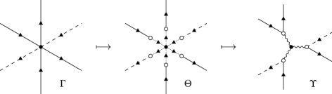
Figure 8.1: A graphical overview of vertex resolution on the level of a single vertex. (We do not draw the other vertices.) In the second step we draw only one of the possible six pairings (in the Hermitian case).

Note that the notion of charged vertex can be lifted from $\Delta$ to $\Gamma$ using the projection $\pi$ (see Definition 8.1 below). The following class of vertices, called marked vertices, plays the central role in this section. Informally, a marked vertex $i\in V_{s}(\Gamma)$ is a charged vertex that, in the construction of $\Gamma$ from $\gamma^{p}(\Delta)$, was linked to by the smallest allowed number of edges (zero if $\pi(i)\notin F$ and one if $\pi(i)\in F$).

Recall that we intend to gain an additional factor $\Phi$ from any charged vertex of $\Gamma$. However, the possibility of doing this may be destroyed if a charged vertex was linked to in the construction of $\Gamma$ from $\gamma^{p}(\Delta)$. In this case we gain from the linking, as always, but we may not additionally gain from the vertex’s being charged. If the vertex was excessively linked (i.e. more than minimally required), then we have the additional gain from this extra linking. Marked vertices are exactly those charged vertices which have been minimally linked. Thus, in order to gain from a marked vertex we cannot use the simple power counting that underlies linking, but need the more refined mechanism of vertex resolution.

Definition 8.1 (Charged and Marked vertices in $\Gamma$).

The set of charged vertices of $\Gamma$ is by definition $V_{c}(\Gamma)\mathrel{\vbox{\hbox{.}\hbox{.}}}=\pi^{-1}(V_{c}(\Delta))$ (see Definition 4.7).

The vertex $i\in V_{c}(\Gamma)$ is called marked if either

1. $\pi(i)\notin F$ and $\deg_{\Gamma}(i)=\deg_{\Delta}(\pi(i))$, or

2. $\pi(i)\in F$ and $\deg_{\Gamma}(i)=\deg_{\Delta}(\pi(i))+2$.

We denote the set of marked vertices by $V_{m}(\Gamma)\subset V_{c}(\Gamma)$.

Note that (i) corresponds to the case where $i$ was not linked to at all, and (ii) to the case where $i$ was linked to exactly once. The following lemma gives a lower bound on the number of edges of $\Gamma$. Informally, it states that if $i$ is not marked but $\pi(i)$ is charged then $i$ was linked to at least once more than the minimum required amount (zero if $\pi(i)\notin F$ and one if $\pi(i)\in F$).

Lemma 8.2.

We have the bound

$$\lvert E(\Gamma)\rvert\;\geqslant\;p(\deg(\Delta)+\lvert F\rvert)+\lvert V_{c}(\Gamma)\rvert-\lvert V_{m}(\Gamma)\rvert\,.$$ (8.1)

Proof.

By definition of $V_{c}(\Gamma)$ and $V_{m}(\Gamma)$, we find that $i\in V_{s}(\Gamma)$ was linked to at least once if

$$i\;\in\;\pi^{-1}(F^{c})\cap V_{c}(\Gamma)\cap V_{m}(\Gamma)^{c}\qquad\text{or}\qquad i\;\in\;\pi^{-1}(F)\cap\bigl{(}{V_{c}(\Gamma)\cap V_{m}(\Gamma)^{c}}\bigr{)}^{c}\,,$$

and $i$ was linked to at least twice if

$$i\;\in\;\pi^{-1}(F)\cap V_{c}(\Gamma)\cap V_{m}(\Gamma)^{c}\,.$$

Since each linking adds an edge to the $p\deg(\Delta)$ edges of $\gamma^{p}(\Delta)$, we find

$$\lvert E(\Gamma)\rvert \;\geqslant\;p\deg(\Delta)+\Bigl{\lvert}\pi^{-1}(F^{c})\cap V_{c}(\Gamma)\cap V_{m}(\Gamma)^{c}\Bigr{\rvert}+\Bigl{\lvert}\pi^{-1}(F)\cap\bigl{(}{V_{c}(\Gamma)\cap V_{m}(\Gamma)^{c}}\bigr{)}^{c}\Bigr{\rvert}$$

$$\mspace{40.0mu}+2\Bigl{\lvert}\pi^{-1}(F)\cap V_{c}(\Gamma)\cap V_{m}(\Gamma)^{c}\Bigr{\rvert}$$

$$\;=\;p\deg(\Delta)+p\lvert F\rvert+p\lvert V_{c}(\Delta)\rvert-\lvert V_{m}(\Gamma)\rvert\,,$$

where in the last step we used that $\pi$ is $p$-to-one and $V_{m}(\Gamma)\subset V_{c}(\Gamma)$. ∎

The goal of this section is to gain an extra factor $\Phi$ from each marked vertex of $\Gamma$ using vertex resolution. Provided we can do this, the proof of Theorem 4.8 will be complete. This can be informally understood as follows. In order to get the estimate (4.7), we need a bound of size $\Psi^{p(\deg(\Delta)+\lvert F\rvert)}\Phi^{p\lvert V_{c}(\Delta)\rvert}$. Each vertex $i\in V_{s}(\Gamma)$ contributes factors $\Psi$ and $\Phi$ (in addition to the trivial $p\deg(\Delta)$) to the estimate as follows.

1. $\pi(i)\notin F$ and $i\notin V_{c}(\Gamma)$. In this case $i$ yields no factor $\Psi$ or $\Phi$.

2. $\pi(i)\notin F$ and $i\in V_{c}(\Gamma)$. If $\deg_{\Gamma}(i)=\deg_{\Delta}(\pi(i))$ then $i$ is marked and will yield a factor $\Phi$ by vertex resolution. If $\deg_{\Gamma}(i)>\deg_{\Delta}(\pi(i))$ then $i$ is not marked but carries an extra factor $\Psi$ since it has been linked to more times than needed. (Thus, $\Gamma$ has at least one extra edge, corresponding to an off-diagonal entry $G_{uv}\prec\Psi$, incident to $i$).

3. $\pi(i)\in F$ and $i\notin V_{c}(\Gamma)$. In this case $i$ has been linked to at least once and is consequently incident to at least one extra edge. This yields a factor $\Psi$.

4. $\pi(i)\in F$ and $i\in V_{c}(\Gamma)$. As in (iii), $i$ has been linked to at least once and hence yields a factor $\Psi$. In addition, $i$ yields a second factor $\Phi$ as follows. If $\deg_{\Gamma}(i)=\deg_{\Delta}(\pi(i))+2$ then $i$ is marked and will yield an extra factor $\Phi$ by vertex resolution. If $\deg_{\Gamma}(i)>\deg_{\Delta}(\pi(i))+2$ then $i$ has been linked to at least twice, hence yielding a second factor $\Psi$. In either case the vertex $i$ generates a factor $\Psi\Phi$.

Thus, from each case (i) – (iv) we gain $\ell_{\Psi}$ factors $\Psi$ and $\ell_{\Phi}$ factors $\Phi$ in addition to the trivially available $p\deg(\Delta)$ factors of $\Psi$, where the values of $\ell_{\Psi}$ and $\ell_{\Phi}$ is as follows: (i) $\ell_{\Psi}=\ell_{\Phi}=0$, (ii) $\ell_{\Psi}=0$, $\ell_{\Phi}=1$, (iii) $\ell_{\Psi}=1$, $\ell_{\Phi}=0$, (iv) $\ell_{\Psi}=\ell_{\Phi}=1$. From this the bound $\Psi^{p(\deg(\Delta)+\lvert F\rvert)}\Phi^{p\lvert V_{c}(\Delta)\rvert}$ follows immediately.

Before moving on to the main argument of this section, we outline how a marked vertex yields an additional factor $\Phi$. We claim that Definitions 4.7 and 8.1 imply that

$$i\in V_{s}(\Gamma)\text{ is marked}\qquad\Longrightarrow\qquad\nu_{i}(\Gamma)\;\neq\;\nu_{i}^{*}(\Gamma)$$ (8.2)

(see Definition 4.6). To see this, let $i$ be an arbitrary marked vertex. If $\pi(i)\notin F$ then by Definition 8.1 $i$ has not been linked to, and hence $\nu_{i}^{\xi}(\Gamma)=\nu_{\pi(i)}^{\xi}(\Delta)$ for $\xi=1,*$. Therefore (8.2) follows from Definition 4.7. On the other hand, if $\pi(i)\in F$ then by Definition 8.1 $i$ has been linked to once, and either (a) $\nu_{i}(\Gamma)=\nu_{\pi(i)}(\Delta)$ and $\nu^{*}_{i}(\Gamma)=\nu^{*}_{\pi(i)}(\Delta)+2$ or (b) $\nu_{i}(\Gamma)=\nu_{\pi(i)}(\Delta)+2$ and $\nu^{*}_{i}(\Gamma)=\nu^{*}_{\pi(i)}(\Delta)$. Either way, Definition 4.7 yields (8.2).

Roughly, vertex resolution splits each summation vertex of degree $2d$ (we assume for simplicity that the vertex is of even degree) into $d$ fresh summation vertices of degree two. If the right-hand side of (8.2) holds (as it does if we are resolving a marked vertex), at least one of the fresh summation vertices will be a chain vertex (i.e. both of its incident edges will have the same colour). The desired gain of a factor $\Phi$ will then come from an application of Proposition 5.3.

8.1.  General graphical representation

Throughout Sections 8 and 9, we shall fix $\bm{\mathrm{a}}$ and apply three algebraic operations to the monomial encoded by $\Gamma$:

1. Family A identities,

2. Family B identities,

3. partial expectation in $\bm{\mathrm{a}}$.

In order to keep track of the structure of the ensuing terms, we make heavy use of graphs. For pedagogical reasons, we shall develop the algebraic and graphical languages in parallel. Each algebraic expression (a monomial in the matrix entries of $G$, $\mathcal{G}$, $H$, and $S$) is represented by a graph. Application of one of the three elementary algebraic identities listed above can, as before, be described by a elementary transformation on graphs. Although the entire argument could be stated in terms of graphs alone, this would rather obscure the underlying mechanism, which always corresponds to applying one of the three algebraic operations listed above. Instead, we introduce each graph operation when it naturally arises in our argument. In order to obtain a set of graphs that is closed under all of the operations we shall need, we extend our set of graphs according to the following definition.

Definition 8.3 (General graph).

By a graph we mean a quintuple $(V_{f},V_{s},V_{e},E,\xi)$ with the following properties. The set $E$ is a set of edges on the vertex set $V\mathrel{\vbox{\hbox{.}\hbox{.}}}=V_{f}\sqcup V_{s}\sqcup V_{e}$. Multiple edges as well as loops are allowed. The colouring $\xi$ is a map

$$\xi\mathrel{\vbox{\hbox{.}\hbox{.}}}E\;\longrightarrow\;\bigl{\{}{\text{solid},\,\text{dashed},\,\text{dotted},\,\text{wiggly}}\bigr{\}}\,.$$

As in Definition 4.1, we sometimes use the alternative notations $\text{solid}\equiv 1$ and $\text{dashed}\equiv*$.

An edge that is solid or dashed is called a resolvent edge. Dotted and resolvent edges are directed, while wiggly edges are undirected. The vertices in $V_{s}$ are called the original summation vertices, in $V_{f}$ the fresh summation vertices, and in $V_{e}$ the external vertices. Vertices in $V_{f}$ are drawn using white dots and vertices in $V_{s}\sqcup V_{e}$ using black dots.

Figure 3.8 contains the dictionary of the colour-code: a solid edge encodes an entry of $G$, a dashed edge an entry of $G^{*}$, a dotted edge an entry of $H$, and a wiggly edge an entry of $S$. More precisely, each resolvent edge encodes a maximally expanded (in ${\bm{\mathrm{a}}}$) resolvent entry (see Definition 6.4), and each dotted edge an $\bm{\mathrm{a}}$-admissible entry of $H$, which is the subject of the following definition.

Definition 8.4.

The entry $h_{uv}$ is an $\bm{\mathrm{a}}$-admissible entry of $H$ if $u\in\bm{\mathrm{a}}$ or $v\in\bm{\mathrm{a}}$.

The arguments below consist of a series of operations on the set of graphs from Definition 8.3. To be completely precise, below we shall in fact adorn the graphs from Definition 8.3 with decorations: resolvent loops may be decorated with a black or white diamond (see Figure 3.3), wiggly edges with an arbitrary number of crossing strokes, and original summation vertices with an arbitrary number of rings. (The latter two concepts are defined above Definition 8.5 and in the beginning of the proof of Lemma 9.3 respectively.)

To each vertex $i\in V(\Gamma)$ of a graph $\Gamma$ we assign an index $u_{i}$. We shall consistently use the splitting

$$\bm{\mathrm{u}}\;=\;(u_{i})_{i\in V(\Gamma)}\;=\;(\bm{\mathrm{x}},\bm{\mathrm{a}},\bm{\mathrm{\mu}})\,,\qquad\bm{\mathrm{x}}\;=\;(x_{i})_{i\in V_{f}(\Gamma)}\,,\qquad\bm{\mathrm{a}}\;=\;(a_{i})_{i\in V_{s}(\Gamma)}\,,\qquad\bm{\mathrm{\mu}}\;=\;(\mu_{i})_{i\in V_{e}(\Gamma)}\,.$$

We say that the index $u_{i}$ is associated with the vertex $i$, and vice versa. We introduce the notation

$$\mathcal{A}(\Gamma)\;\equiv\;\mathcal{A}_{\bm{\mathrm{a}},\bm{\mathrm{x}}}(\Gamma)$$ (8.3)

for the monomial (in the entries of $G^{(T)}$, $\mathcal{G}^{(T)}$, $H$, and $S$ where $T\subset\bm{\mathrm{a}}$) encoded by the graph $\Gamma$. Note that $\mathcal{A}(\Gamma)$ has an explicit formula, analogous to (4.2) except needing much heavier notation. As we shall not need it, we shall not give it. (Note also that our graphs do not keep track of any factors of $Q$, as we shall not need this information.)

8.2.  Generation of the fresh summation vertices

Next, we define the vertex resolution operation precisely. Our starting point is a fixed $\Gamma\in\mathfrak{G}_{F}^{p}(\Delta)$. In order to streamline the argument, we at first make the following simplifying assumption on $\Delta$, which is removed in Section 9.

• There are no diagonal entries $\mathcal{G}_{aa}=G_{aa}-m$ in $\mathcal{Z}(\Delta)$. (I.e. $\Delta$ has no loops.)

The operation of vertex resolution consists of two main steps: the generation and lumping of fresh summation vertices. The idea behind the first step – the generation of fresh summation vertices – is to resolve, using the Family B identities (3.14a) and (3.14b), each (already maximally expanded) off-diagonal resolvent entry $G_{uv}^{(\bm{\mathrm{a}}\setminus\{u,v\})}$, with $u\neq v$, in any summation index from the set $\{u,v\}$. (The word “resolve” here refers to explicitly identifying the dependence on all matrix entries $h_{ij}$ with $i,j\in\bm{\mathrm{a}}$ so that partial expectation in these variables can be taken. After taking the partial expectation, we shall get expressions that can again be represented by admissible graphs.) More precisely, we write

$$G^{(\bm{\mathrm{a}}\setminus\{u,v\})}_{uv}\;=\;\begin{cases}-G_{uu}^{(\bm{\mathrm{a}}\setminus\{u\})}\sum_{x}^{(\bm{\mathrm{a}})}h_{ux}G_{xv}^{(\bm{\mathrm{a}})}&\text{($u$ summation and $v$ external)}\,,\\ -G_{vv}^{(\bm{\mathrm{a}}\setminus\{v\})}\sum_{x}^{(\bm{\mathrm{a}})}G_{ux}^{(\bm{\mathrm{a}})}h_{xv}&\text{($u$ external and $v$ summation)}\,,\\ G_{uu}^{(\bm{\mathrm{a}}\setminus\{u,v\})}G_{vv}^{(\bm{\mathrm{a}}\setminus\{v\})}\bigl{(}{-h_{uv}+\sum_{x,y}^{(\bm{\mathrm{a}})}h_{ux}G_{xy}^{(\bm{\mathrm{a}})}h_{xv}}\bigr{)}&\text{($u$ and $v$ summation)}\,.\end{cases}$$ (8.4)

(As stated after Definition 4.1, we exclude the trivial case where both $u$ and $v$ are external indices.) The proof of (8.4) is a straightforward consequence of the identities (3.14a) and (3.14b), and the fact that $u\neq v$ by definition of $X_{F}^{w}(\Delta)$. For example, if $a$ and $b$ are summation indices and $\mu$ and $\nu$ are external indices, we write

$$G_{\mu a}^{(b)}G_{ab}G_{b\mu}^{(a)*}G_{a\nu}^{(b)}G_{\nu a}^{(b)*}\\ =\;G_{aa}^{(b)}G_{aa}G_{bb}^{(a)}G_{bb}^{(a)*}G_{aa}^{(b)}G_{aa}^{(b)*}\sum_{x,y,z,u,v,w}^{(ab)}G_{\mu x}^{(ab)}h_{xa}h_{ay}G^{(ab)}_{yz}h_{zb}h_{bu}G_{u\mu}^{(ab)*}h_{av}G^{(ab)}_{v\nu}G_{\nu w}^{(ab)*}h_{wa}\\ -G_{aa}^{(b)}G_{aa}G_{bb}^{(a)}G_{bb}^{(a)*}G_{aa}^{(b)}G_{aa}^{(b)*}\sum_{x,u,v,w}^{(ab)}G_{\mu x}^{(ab)}h_{xa}h_{ab}h_{bu}G_{u\mu}^{(ab)*}h_{av}G^{(ab)}_{v\nu}G_{\nu w}^{(ab)*}h_{wa}\,.$$ (8.5)

Notice that along this procedure we may generate non-maximally expanded diagonal terms, (e.g. $G_{aa}$ above), but off-diagonal terms always have upper indices $\bm{\mathrm{a}}$. Moreover, all entries of $H$ on the right-hand side of (8.5) are $\bm{\mathrm{a}}$-admissible.

At this point we make the following further simplification, which leaves the essence of the argument unchanged but removes some technicalities.

• We replace any diagonal term $G_{aa}^{(T)}$ with $m$ and any diagonal term $G_{aa}^{(T)*}$ with $\bar{m}$. (Recall that $G_{aa}^{(T)}\approx m$ in the sense that $G_{aa}^{(T)}-m\prec\Psi$ by definition of $\Lambda$.) This replacement is done in two places: in $\mathcal{A}(\Gamma)$ and in the identities (3.14a) and (3.14b) which underlie the algebra of vertex resolution.

Again, Simplification (S3) is removed in Section 9. Thus, under Simplification (S3), we neglect all diagonal terms in (8.5). (More precisely, we replace each one of them with $m$ or $\bar{m}$; the resulting powers of $m$ and $\bar{m}$ are irrelevant for estimates by (3.11).)

The use of graphs greatly simplifies the analysis of complicated expressions like (8.5). The identities (8.4) all have obvious graphical representations. In Figure 8.2 we give a graphical depiction of (8.5). (Recall the conventions introduced in Figure 3.8.) In the typical case, the summation vertex of degree four associated with $a$ gives rise to four fresh summation vertices, associated with $x,y,v,w$; likewise the summation vertex of degree two associated with $b$ creates two fresh vertices associated with $u$ and $z$ (first term in the right side of (8.5)). Due to presence of the term $h_{uv}$ in (8.4), sometimes two summation indices are directly connected with a dotted line at the expense of one fewer fresh summation vertex adjacent to each of these two indices. This results in the second term on the right-hand side of (8.5), which contains a factor $h_{ab}$ (note that $G_{ab}$ plays the role of $G_{uv}^{\bm{\mathrm{a}}\setminus\{u,v\}}$ from (8.4)).

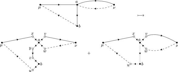
Figure 8.2: The vertex resolution from (8.5). The graph $\Gamma$ is represented on the top and both graphs of $\widetilde{\mathfrak{R}}(\Gamma)$ are represented on the bottom. In accordance with Simplification (S3) we do not draw the diagonal entries of $G$.

The generation of fresh summation vertices for a general $\Gamma\in\mathfrak{G}_{F}^{p}(\Delta)$ is no different from the above example. Applying the graphical rules associated with (8.4) to each edge of $\Gamma$, we get a finite family of graphs which we denote by $\widetilde{\mathfrak{R}}(\Gamma)$. In accordance with Simplifications (S2) and (S3), in this section we drop all diagonal terms, and hence all loops from the graphs in $\widetilde{\mathfrak{R}}(\Gamma)$. (In Section 9 below we keep track of the loops, which will lead to the larger set $\mathfrak{R}$.)

Any graph $\Theta\in\widetilde{\mathfrak{R}}(\Gamma)$ has the following properties.

1. $\Theta$ has only straight, dashed or dotted edges but no wiggly edge (see Figure 3.8).

2. $\Theta$ has no loops or multiple edges.

3. The sets $V_{s}(\Theta)=V_{s}(\Gamma)$ and $V_{e}(\Theta)=V_{e}(\Gamma)$ remain unchanged, as do the associated indices $\bm{\mathrm{a}}$ and $\bm{\mathrm{\mu}}$. In addition, we now have a new set of vertices, $V_{f}(\Theta)\neq\emptyset$, which indexes the fresh summation vertices $\bm{\mathrm{x}}$.

4. Each resolvent edge of $\Theta$ encodes an entry of $G^{(\bm{\mathrm{a}})}$ or $G^{(\bm{\mathrm{a}})*}$ in $\mathcal{A}(\Theta)$ (in particular, no resolvent edge of $\Theta$ is incident to $V_{s}(\Theta)$). Each dotted edge of $\Theta$ encodes an $\bm{\mathrm{a}}$-admissible entry of $H$ in $\mathcal{A}(\Theta)$.

5. For $i,j\in V_{s}(\Theta)$ let the symmetric function $\sigma(i,j)$ denote the number of dotted edges joining $i$ and $j$. The number of edges in $\Gamma$ and $\Theta$ is conserved in the sense that

   $$\lvert E(\Gamma)\rvert\;=\;\sum_{e\in E(\Theta)}\bigl{(}{\bm{\mathrm{1}}(\xi_{e}=1)+\bm{\mathrm{1}}(\xi_{e}=*)}\bigr{)}+\frac{1}{2}\sum_{i,j\in V_{s}(\Theta)}\sigma(i,j)\,.$$ (8.6)

   Informally: in the process $\Gamma\mapsto\Theta$ that generates fresh summation vertices, each resolvent entry either remains a resolvent entry or is replaced with an entry of $H$ with original summation vertices. This simply corresponds to the two terms in the last line of the right-hand side of (8.4).

6. Each original summation vertex is incident only to dotted edges.

7. Each fresh summation vertex has degree two and is incident to precisely one dotted edge.

We remark that, by construction, the sets $\bm{\mathrm{x}}$ and $\bm{\mathrm{a}}$ are disjoint, as are the sets $\bm{\mathrm{a}}$ and $\bm{\mathrm{\mu}}$. However, $\bm{\mathrm{x}}$ and $\bm{\mathrm{\mu}}$ are in general not disjoint, and indices of $\bm{\mathrm{x}}$ may coincide.

8.3.  Lumping of the fresh summation vertices

We now take the expectation of $\mathcal{A}(\Theta)$. In fact, all that we shall need is the partial expectation in $\bm{\mathrm{a}}$. The key observation is that, by Property (iv) in Section 8.2, each resolvent entry of $\mathcal{A}(\Theta)$ is independent of $\bm{\mathrm{a}}$ and each entry of $H$ is $\bm{\mathrm{a}}$-admissible. In particular, the partial expectation $\prod_{a\in\bm{\mathrm{a}}}P_{a}$ acting on $\mathcal{A}(\Theta)$ acts on the product of the entries of $H$ alone. Since this product is an explicit monomial, we can evaluate its expectation directly. If the random variables $h_{uv}$ were Gaussian, this would correspond to a simple Wick-pairing of the dotted edges. Pairing two dotted edges, each of them incident to a fresh summation vertex and a common original summation vertex, results in a pairing of two fresh summation vertices. Since $\bm{\mathrm{x}}$ and $\bm{\mathrm{a}}$ are distinct, a dotted edge incident to a fresh summation vertex cannot be paired with a dotted edge incident to two original summation vertices. In the non-Gaussian case, higher-order moments are also present, but they are suppressed by a combinatorial factor (i.e. a positive power of $M^{-1}$). Graphically, we represent the procedure of taking expectation by pairing (or in general lumping) fresh summation indices, and replace the corresponding doubled dotted line by a wiggly line. What follows is a more precise description.

We define the second step of vertex resolution – the lumping of the fresh summation vertices. Before giving the general procedure, we complete the analysis of the example (8.5). From (8.5), assuming Simplification (S3), we get

$$\mathbb{E}G_{\mu a}^{(b)}G_{ab}G_{b\mu}^{(a)*}G_{a\nu}^{(b)}G_{\nu a}^{(b)*}$$

$$\mspace{30.0mu}\overset{\mathrm{{\bf(S3)}}}{=}\;m^{4}\bar{m}^{2}\sum_{x,y,z,u,v,w}^{(ab)}\mathbb{E}G_{\mu x}^{(ab)}G^{(ab)}_{yz}G_{u\mu}^{(ab)*}G^{(ab)}_{v\nu}G_{\nu w}^{(ab)*}P_{a}\bigl{(}{h_{xa}h_{ay}h_{av}h_{wa}}\bigr{)}P_{b}(h_{zb}h_{bu})$$

$$\mspace{50.0mu}-m^{4}\bar{m}^{2}\sum_{x,u,v,w}^{(ab)}\mathbb{E}G_{\mu x}^{(ab)}G_{u\mu}^{(ab)*}G^{(ab)}_{v\nu}G_{\nu w}^{(ab)*}h_{av}h_{wa}h_{xa}P_{b}\bigl{(}{h_{ab}h_{bu}}\bigr{)}\,,$$ (8.7)

where we used the trivial identity $\mathbb{E}X=\mathbb{E}P_{a}P_{b}X$ and the fact that $G^{(ab)}$ is independent of $a$ and $b$ (see Definition 2.3). Since $a\neq u$, the partial expectation $P_{b}$ on the second line of (8.7) vanishes. The partial expectations on the first line of (8.7) may be computed explicitly, similarly to the computation (3.38):

$$P_{a}\bigl{(}{h_{xa}h_{ay}h_{av}h_{wa}}\bigr{)}P_{b}(h_{zb}h_{bu})\\ =\;s_{ax}s_{av}s_{bz}\delta_{xy}\delta_{vw}\delta_{zu}+s_{ax}s_{ay}s_{bz}\delta_{xv}\delta_{yw}\delta_{zu}+\bm{\mathrm{1}}(x=y=v=w)s_{ax}^{2}s_{bz}\delta_{zu}\mathbb{E}\lvert\zeta_{ax}\rvert^{4}\,.$$

Here we assumed the condition (3.21). In the case (3.20), we get the additional term

$$s_{ax}s_{ay}\delta_{xw}s_{bz}\delta_{yv}\delta_{zu}\,.$$

Thus we may write (in the case (3.21) for simplicity)

$$\mathbb{E}G_{\mu a}^{(b)}G_{ab}G_{b\mu}^{(a)*}G_{a\nu}^{(b)}G_{\nu a}^{(b)*} \;\overset{\mathrm{{\bf(S3)}}}{=}\;m^{4}\bar{m}^{2}\mathbb{E}\sum_{x,v,z}^{(ab)}s_{ax}s_{av}s_{bz}\,G_{\mu x}^{(ab)}G^{(ab)}_{xz}G_{z\mu}^{(ab)*}G^{(ab)}_{v\nu}G_{\nu v}^{(ab)*}$$

$$\mspace{30.0mu}+m^{4}\bar{m}^{2}\mathbb{E}\sum_{x,y,z}^{(ab)}s_{ax}s_{ay}s_{bz}\,G_{\mu x}^{(ab)}G^{(ab)}_{yz}G_{z\mu}^{(ab)*}G^{(ab)}_{x\nu}G_{\nu y}^{(ab)*}$$

$$\mspace{30.0mu}+m^{4}\bar{m}^{2}\mathbb{E}\sum_{x,z}^{(ab)}s_{ax}^{2}s_{bz}\bigl{(}{\mathbb{E}\lvert\zeta_{ax}\rvert^{4}}\bigr{)}\,G_{\mu x}^{(ab)}G^{(ab)}_{xz}G_{z\mu}^{(ab)*}G^{(ab)}_{z\nu}G_{\nu x}^{(ab)*}\,.$$ (8.8)

Note that the summations on the right-hand side are performed with respect to weights (see Definition 4.4). Now it is apparent how better estimates are available for each term on the right-hand side than the term on the left-hand side. Indeed, all terms contain five off-diagonal entries of $G$. In addition, however, the first two terms on the right-hand side contain a summation index associated with a chain vertex $x$ (see Definition 5.1) which is summed over with respect to the chain weight $s_{ax}$ (see Definition 5.2). The last term is suppressed by an additional factor $s_{ax}\leqslant M^{-1}$. Invoking Proposition 5.3 (and neglecting the upper indices $(ab)$ which are dealt with easily in the full proof below), we find that the arguments of $\mathbb{E}$ on the right-hand side of (8.8) are all $O_{\prec}(\Psi^{5}\Phi)$. Here the extra factor $\Phi$ was extracted from the resolution of the vertex $i$ associated with the summation variable $a$, and arose from the fact that $\nu_{i}(\Gamma)\neq\nu_{i}^{*}(\Gamma)$.

Again, the lumping of fresh summation vertices is best represented graphically. In order to represent terms like the last term on the right-hand side of (8.8) graphically, we represent the expression $\mathbb{E}\lvert h_{ij}\rvert^{2+k}$ using a wiggly line crossed by $k$ strokes. Thus, a wiggly edge may be either uncrossed or crossed. We shall always use the bound

$$P_{i}\lvert h_{ij}\rvert^{2+k}\;=\;s_{ij}^{1+k/2}\mathbb{E}\lvert\zeta_{ij}\rvert^{2+k}\;\leqslant\;s_{ij}M^{-k/2}$$

in combination with crossed wiggly lines. See Figure 8.3 for a graphical depiction of (8.8).

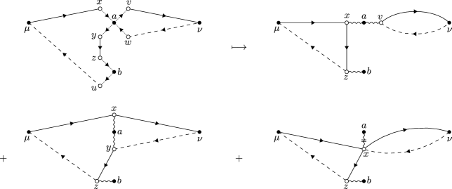
Figure 8.3: The lumping of the fresh summation vertices in the example (8.5). The graph on the left-hand side is $\Theta$ (representing the first term on the right-hand side of (8.7)), and the three graphs on the right-hand side are the elements of $\mathfrak{L}(\Theta)$ (representing the three terms on the right-hand side of (8.8)).

The general case is similar to the example (8.8).

Definition 8.5 (Lumping).

A lumping is a partition whose blocks, called lumps, have size greater than or equal to two.

Let $\Gamma\in\mathfrak{G}_{F}^{p}(\Delta)$ and $\Theta\in\widetilde{\mathfrak{R}}(\Gamma)$. From $\Theta$ we generate a finite family of graphs $\Upsilon$ by taking all lumpings of the white vertices (fresh summation vertices) of $\Theta$. (This lumping, or identification of vertices, arises from taking the partial expectation $\prod_{a\in\bm{\mathrm{a}}}P_{a}$ of all entries of $H$ in $\mathcal{A}(\Theta)$. Note that each fresh summation vertex of $\Theta$ must be lumped with at least another one because $h_{ij}$ and $h_{kl}$ are independent if $\{i,j\}\neq\{k,l\}$, and $P_{i}h_{ij}=0$.) Thus, the result of the lumping is to merge some white vertices into lumps, where each lump consists of at least two vertices, and is again represented as a single white vertex. We denote by $\mathfrak{L}(\Theta)$ the set of such graphs $\Upsilon$ obtained by lumping the fresh summation vertices of $\Theta$. Recall that all resolvent matrix entries encoded by the resolvent edges of $\Theta$ have upper indices $\bm{\mathrm{a}}$. Hence any factors $Q_{a}$ with $a\in\bm{\mathrm{a}}$ act trivially on them according to the identity $Q_{a}\bigl{(}{G^{(\bm{\mathrm{a}})}_{ij}X}\bigr{)}=G^{(\bm{\mathrm{a}})}_{ij}Q_{a}X$ for all $a\in\bm{\mathrm{a}}$. Therefore the factors $Q$ only act on entries of $H$. As in the example (3.36), they simply forbid some pairings; this restriction is no importance for us, and we shall estimate the contribution of arbitrary pairings. Note that after the partial expectation in $\bm{\mathrm{a}}$ has been taken, no factors $Q$ remain. In particular, $\mathcal{A}(\Upsilon)$ has no factors $Q$.

Any graph $\Upsilon\in\mathfrak{L}(\Theta)$ has the following properties.

1. $\Upsilon$ has no loops or multiple edges.

2. The vertex set of $\Upsilon$ is a disjoint union $V(\Upsilon)=V_{f}(\Upsilon)\sqcup V_{s}(\Upsilon)\sqcup V_{e}(\Upsilon)$, where $V_{s}(\Upsilon)=V_{s}(\Theta)=V_{s}(\Gamma)$ is the set of original summation vertices, and $V_{e}(\Upsilon)=V_{e}(\Theta)=V_{e}(\Gamma)$ is the set of external summation vertices. (The set of fresh summation vertices $V_{f}(\Upsilon)$ is strictly smaller than $V_{f}(\Theta)$.)

3. A directed edge $(i,j)$ of $\Theta$ has one of two colours: solid (encoding $G_{ij}^{(\bm{\mathrm{a}})}$) or dashed (encoding $G_{ij}^{(\bm{\mathrm{a}})*}$). An undirected edge is always wiggly. An uncrossed wiggly edge $\{i,j\}$ encodes $\mathbb{E}\lvert h_{ij}\rvert^{2}=s_{ij}$, and a wiggly edge $\{i,j\}$ crossed by $k$ strokes encodes $\mathbb{E}\lvert h_{ij}\rvert^{2+k}=s_{ij}^{1+k/2}\mathbb{E}\lvert\zeta_{ij}\rvert^{2+k}$.

4. Each $i\in V_{f}(\Upsilon)$ is adjacent (via a wiggly line) to a unique vertex $p(i)\in V_{s}(\Upsilon)$. Thus, the map $p\mathrel{\vbox{\hbox{.}\hbox{.}}}V_{f}(\Upsilon)\to V_{s}(\Upsilon)$ is a projection which associates with each fresh summation vertex $i$ its “parent” original summation vertex $p(i)$. (E.g. in the first graph on the right-hand side of Figure 8.3 we have $p(x)=p(v)=a$ and $p(z)=b$.)

5. For each $i,j\in V_{s}(\Upsilon)$, we have $\sigma(i,j)\in\{0,2,3,4,\dots\}$. (Recall that $\sigma(i,j)$ is the number of dotted lines in the graph $\Theta$ between vertices $i,j\in V_{s}(\Upsilon)=V_{s}(\Theta)$.) If $\sigma(i,j)\geqslant 2$ then $i$ and $j$ are connected by a wiggly line crossed by $\sigma(i,j)-2$ strokes. Moreover, the number of edges is conserved in the sense that

   $$\lvert E(\Gamma)\rvert\;=\;\sum_{e\in E(\Upsilon)}\bigl{(}{\bm{\mathrm{1}}(\xi_{e}=1)+\bm{\mathrm{1}}(\xi_{e}=*)}\bigr{)}+\frac{1}{2}\sum_{i,j\in V_{s}(\Upsilon)}\sigma(i,j)\,,$$ (8.9)

   as follows from (8.6).

See Figure 8.4 for an illustration of (v).

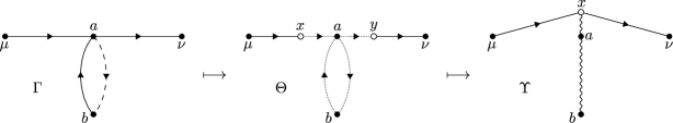
Figure 8.4: The resolution process $\Gamma\mapsto\Theta\mapsto\Upsilon$, where in the first step we chose a $\Theta$ satisfying $\sigma(i,j)=2$ where $i$ and $j$ are the original summation vertices associated with $a$ and $b$ respectively. This figure illustrates the property (v) above, as well as the conservation of the number of edges from (8.6) and (8.9).

8.4.  Summing over the fresh summation indices and completion of the proof

The complete process of vertex resolution may be summarized as

$$\Gamma\in\mathfrak{G}_{F}^{p}(\Delta)\quad\longmapsto\quad\Theta\in\widetilde{\mathfrak{R}}(\Gamma)\quad\longmapsto\quad\Upsilon\in\mathfrak{L}(\Theta)\,.$$

Here the first step represents explicitly resolving all maximally expanded entries of $G$ (encoded by resolvent edges of $\Gamma$) in $\bm{\mathrm{a}}$-admissible entries of $H$. The second step represents taking partial expectation in all these $h$-variables.

At this point, we introduce a further, and final, simplification that allows us to postpone some needless technicalities to Section 9.

• The sets $\bm{\mathrm{x}}=(x_{i})_{i\in V_{f}(\Upsilon)}$ and $\bm{\mathrm{\mu}}=(\mu_{i})_{i\in V_{e}(\Upsilon)}$ are disjoint, and all indices of $\bm{\mathrm{x}}$ are distinct.

Thus, Simplification (S4) is in the same spirit as Simplification (S1). We assume Simplification (S4) throughout Section 8.4.

Let $\Gamma\in\mathfrak{G}_{F}^{p}(\Delta)$, $\Theta\in\widetilde{\mathfrak{R}}(\Gamma)$, and $\Upsilon\in\mathcal{L}(\Theta)$. Choose and fix a marked vertex $i\in V_{m}(\Gamma)$ (see Definition 8.1). In order to gain an extra factor $\Phi$ from $i$, we consider three cases, (a), (b), and (c).

First we explain them informally. Case (a) is the typical situation. Since $i$ is marked, it is a charged vertex in $\Delta$, i.e. after having been minimally linked to, the number of solid and dashed edges adjacent to it are different. In case (a) we show that this property is inherited by at least one of the fresh summation vertices whose parent is $i$. This fact is fairly clear since neither vertex generation nor lumping alters the number of solid or dashed edges. This will imply that one fresh summation vertex generated by $i$ is a chain vertex in $\Upsilon$; this in turn will give the extra factor $\Phi$ associated with $i\in V_{m}(\Gamma)$. The other two cases represent exceptional cases. Case (b) deals with a higher-order lumping (i.e. a lumping which has a lump of size greater than two). As indicated above, this results in a combinatorial gain expressed in terms of powers of $M^{-1}$. Such a factor is depicted graphically using a crossed wiggly line. Finally, case (c) deals with the consequence of the factor $h_{uv}$ on the last line of (8.4), i.e. when a dotted edge joins two original summation vertices. We note that choosing the term $h_{uv}$ is the only way to change the number of solid or dashed edges (off-diagonal entries of $G$) in the process of vertex resolution. Since dotted edges must be paired, we find that at least two parallel solid or dashed edges must be replaced with a dotted edge; this corresponds to replacing two off-diagonal factors $G_{uv}$ with $\lvert h_{uv}\rvert^{2}$. After expectation, this means trading in a factor $\Psi^{2}$ for $M^{-1}$. Since $\Psi\Phi\geqslant M^{-1/2}$, the factor $M^{-1}$ may be estimated by $\Psi^{2}\Phi^{2}$. Out of this, $\Psi^{2}$ is used to compensate for the loss of $\Psi^{2}$ mentioned above (losing two off-diagonal entries of $G$), and the remaining $\Phi^{2}$ provides us with the gains of $\Phi$ associated with each of the two vertices incident to the dotted edge. See Figure 8.5 for a graphical depiction of the cases (a), (b), and (c). Below we formalize these ideas.

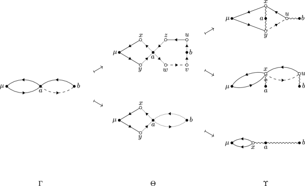
Figure 8.5: A simple example of vertex resolution giving rise to the three cases (a), (b), and (c) when resolving the vertex associated with $a$. From top to bottom in the right-hand column: cases (a), (b), and (c). In the top graph, corresponding to case (a), $x$ is a chain vertex (within the chain $u\to x\to\mu$) which is a remnant of the path $b\to a\to\mu$ consisting of solid edges in the graph $\Gamma$. In the middle graph, corresponding to case (b), the crossed wiggly line expresses that all four fresh summation indices arising from the resolution of $a$ coincide, and the four associated dotted edges of $\Theta$ were collapsed into one of $\Upsilon$. Finally, in the bottom figure, corresponding to case (c), the solid and dashed edges between the vertices associated with $a$ and $b$ in $\Gamma$ give rise to a single wiggly line according to $s_{ab}=\mathbb{E}\lvert h_{ab}\rvert^{2}$.

Recall the definitions of $\nu_{i}$ and $\nu_{i}^{*}$ for an arbitrary edge-coloured, directed multigraph (Definition 4.6). Informally, $\nu_{i}^{\xi}$ gives the number of legs of colour $\xi$ incident to $i$. The following definition gives a natural extension of chain weights to graphs with wiggly edges.

Definition 8.6.

A vertex $i\in V_{f}(\Upsilon)$ is a chain vertex if it has degree three, such that: (i) $i$ is incident to exactly one wiggly edge, and (ii) $i$ is incident to exactly two resolvent edges, which are of the same colour.

Thus a chain vertex $i\in V_{f}(\Upsilon)$ corresponds to a chain vertex in the sense of Definition 4.6 (i.e. $\nu_{i}(\Upsilon)+\nu_{i}^{*}(\Upsilon)=2$ and one of the terms vanishes), with the added condition that the summation over the index of $i$ is done with respect to a chain weight (encoded in $\mathcal{A}(\Upsilon)$ by the wiggly edge of $\Upsilon$ incident to $i$).

Now we present the details of the cases (a), (b), and (c). Let $\Gamma\in\mathfrak{G}_{F}^{p}(\Delta)$, $\Theta\in\widetilde{\mathfrak{R}}(\Gamma)$, and $\Upsilon\in\mathcal{L}(\Theta)$. Let $i\in V_{m}(\Gamma)$ be marked.

• Suppose that $\sigma(i,j)=0$ for all $j\in V_{s}(\Upsilon)$ (i.e. there are no wiggly edges in $\Upsilon$ that join two original summation vertices). Suppose moreover that the lumping of the fresh summation vertices of $p^{-1}(i)$ that generates $\Upsilon$ is a pairing (hence $\deg_{\Gamma}(i)$ must be even).

  Then $\nu_{j}(\Upsilon)+\nu_{j}^{*}(\Upsilon)=2$ for any $j\in p^{-1}(i)$. More precisely, each $j\in p^{-1}(i)$ has degree three in $\Upsilon$; two of the incident edges are resolvent edges, and the third edge is a wiggly uncrossed edge connecting $j$ with $i$. Moreover,

  $$\nu_{i}^{\xi}(\Gamma)\;=\;\sum_{j\in p^{-1}(i)}\nu_{j}^{\xi}(\Upsilon)$$ (8.10)

  for $\xi=1,*$, since, under the assumption that there are no wiggly edges in $\Upsilon$ that join two original summation vertices, the total number of resolvent edges incident to $i$ does not change by vertex resolution and taking expectation. Hence we find from (8.2) and from $\nu_{j}(\Upsilon)+\nu_{j}^{*}(\Upsilon)=2$ that there must exist a $j\in p^{-1}(i)$ such that either $\nu_{j}(\Upsilon)=0$ or $\nu_{j}^{*}(\Upsilon)=0$; this implies that $j$ is a chain vertex of $\Upsilon$. We conclude:

  At least one $j\in p^{-1}(i)$ is a chain vertex of $\Upsilon$.

• Suppose that $\sigma(i,j)=0$ for all $j\in V_{s}(\Upsilon)$, and the lumping of the fresh summation vertices of $p^{-1}(i)$ that generates $\Upsilon$ is a not pairing.

  In this case one fresh summation vertex $j\in p^{-1}(i)$ was obtained by lumping together three or more fresh summation vertices of $\Theta$. We conclude:

  At least one $j\in p^{-1}(i)$ is connected in $\Upsilon$ to $i$ by a crossed wiggly edge.

• Suppose that $\sigma(i,j)>0$ for some $j\in V_{s}(\Gamma)$. By property (v) of Section 8.3, $\sigma(i,j)\geqslant 2$. By construction of $\Upsilon$, if $\sigma(i,j)\geqslant 2$ then $i$ is joined to $j$ in $\Upsilon$ by a wiggly edge that is crossed by $\sigma(i,j)-2$ strokes. We conclude:

  The vertex $i$ is connected in $\Upsilon$ to some $j\in V_{s}(\Upsilon)$ by a wiggly edge.

Partition $V_{m}(\Gamma)=V_{m}^{(a)}\sqcup V_{m}^{(b)}\sqcup V_{m}^{(c)}$ into three subsets according to the three case (a), (b), and (c). Now we may estimate the contribution of $\Upsilon$. For the whole estimate we freeze the original summation vertices $\bm{\mathrm{a}}$. We shall use Proposition 5.3 on the $\lvert V_{m}^{(a)}\rvert$ chain vertices of $\Upsilon$. In order to do so, we still have to get rid of the upper indices $(\bm{\mathrm{a}})$ from each resolvent entry. This is done exactly as in the end of Section 7.1, using the identity (7.3). We omit further details. Thus Proposition 5.3 is applicable to each chain vertex of $\Upsilon$. The remainder of the proof is a simple counting of different types of vertices.

Let

$$\sigma\;\mathrel{\vbox{\hbox{.}\hbox{.}}}=\;\frac{1}{2}\sum_{i,j\in V_{s}(\Theta)}\sigma(i,j)$$

denote the number of dotted edges of $\Theta$ that join two vertices in $V_{s}(\Theta)$. From (8.9) we find that $\Upsilon$ has $\lvert E(\Gamma)\rvert-\sigma$ resolvent edges. Moreover, $\Upsilon$ has $\lvert V_{m}^{(a)}\rvert$ chain vertices. The gain from cases (b) and (c) is as follows. From the vertices of type (b) we gain $M^{-\lvert V_{m}^{(b)}\rvert/2}$. (Each such vertex is incident to a crossed wiggly line, and dropping the strokes crossing such a lines yields a factor $M^{-1/2}$.) From the vertices of type (c) we gain $M^{-\sigma/2}$. (Each dotted edge, encoding $h_{uv}=(s_{uv})^{1/2}\zeta_{uv}$, yields a contribution of size $(s_{uv})^{1/2}\leqslant CM^{-1/2}$ after taking the expectation in the $h$-variables.)

Now we sum over $\bm{\mathrm{x}}$ (while still keeping $\bm{\mathrm{a}}$ frozen). Invoking Proposition 5.3 to estimate the chain vertices of $\Upsilon$, we therefore find that the contribution of $\Upsilon$ is bounded by

$$\mathcal{X}\;\mathrel{\vbox{\hbox{.}\hbox{.}}}=\;\Psi^{\lvert E(\Gamma)\rvert-\sigma}\,\Phi^{\lvert V_{m}^{(a)}\rvert}\,M^{-\lvert V_{m}^{(b)}\rvert/2}\,M^{-\sigma/2}\;\leqslant\;\Psi^{\lvert E(\Gamma)\rvert-\sigma}\,\Phi^{\lvert V_{m}^{(a)}\rvert+\lvert V_{m}^{(b)}\rvert}\,M^{-\sigma/2}\,,$$

where we used $M^{-1/2}\leqslant\Phi$. Since $\sigma(i,j)\geqslant 2$ in case (c), it is easy to see that $\lvert V_{m}^{(c)}\rvert\leqslant\sigma$. Thus we have $\lvert V_{m}^{(a)}\rvert+\lvert V_{m}^{(b)}\rvert+\sigma\geqslant\lvert V_{m}(\Gamma)\rvert$. This yields the bound

$$\mathcal{X}\;\leqslant\;\Psi^{\lvert E(\Gamma)\rvert}\Phi^{\lvert V_{m}^{(a)}\rvert+\lvert V_{m}^{(b)}\rvert+\sigma}\,\bigl{(}{\Psi^{-1}\Phi^{-1}M^{-1/2}}\bigr{)}^{\sigma}\;\leqslant\;\Psi^{\lvert E(\Gamma)\rvert}\Phi^{\lvert V_{m}(\Gamma)\rvert}\,,$$

where we also used that $\Psi\Phi\geqslant M^{-1/2}$. Recalling Lemma 8.2, we find

$$\mathcal{X}\;\leqslant\;\Psi^{p(\deg(\Delta)+\lvert F\rvert)+\lvert V_{c}(\Gamma)\rvert-\lvert V_{m}(\Gamma)\rvert}\,\Phi^{\lvert V_{m}(\Gamma)\rvert}\;\leqslant\;\Psi^{p(\deg(\Delta)+\lvert F\rvert)}\,\Phi^{p\lvert V_{c}(\Delta)\rvert}\,,$$ (8.11)

where we used $\lvert V_{m}(\Gamma)\rvert\leqslant\lvert V_{c}(\Gamma)\rvert=p\lvert V_{c}(\Delta)\rvert$ and $\Psi\leqslant\Phi$. This estimate was obtained for the sum over $\bm{\mathrm{x}}$ with fixed $\bm{\mathrm{a}}$. Finally, we sum over $\bm{\mathrm{a}}$ trivially, using the fact the $\bm{\mathrm{a}}$-summation is performed with respect to a weight. This concludes the proof of Theorem 4.8 under Simplifications (S1) – (S4).

9 Removing Simplifications (S1) – (S4)

In this section we go back to the proof of Theorem 4.8 of Section 8, and give the additional arguments required to remove the Simplifications (S1) – (S4) which were assumed there. For ease of reference, we recall them here.

• All summation indices in the expanded summation $\mathbb{E}\lvert X_{F}^{w}(\Delta)\rvert^{p}$ (see (6.5) below) are distinct. (I.e. we ignore repeated indices which give rise to a smaller combinatorics of the summation.)

• There are no diagonal entries $\mathcal{G}_{aa}=G_{aa}-m$ in $\mathcal{Z}(\Delta)$. (I.e. $\Delta$ has no loops.)

• We replace any diagonal term $G_{aa}^{(T)}$ with $m$ and any diagonal term $G_{aa}^{(T)*}$ with $\bar{m}$. (Recall that $G_{aa}^{(T)}\approx m$ in the sense that $G_{aa}^{(T)}-m\prec\Psi$ by definition of $\Lambda$.) This replacement is done in two places: in $\mathcal{A}(\Gamma)$ and in the identities (3.14a) and (3.14b) which underlie the algebra of vertex resolution.

• The families $\bm{\mathrm{x}}=(x_{i})_{i\in V_{f}(\Upsilon)}$ and $\bm{\mathrm{\mu}}=(\mu_{i})_{i\in V_{e}(\Upsilon)}$ are disjoint, and all indices of $\bm{\mathrm{x}}$ are distinct.

9.1.  Removing Simplification (S3)

We start by removing Simplification (S3), while still assuming Simplifications (S1), (S2), and (S4). In order to remove Simplification (S3), we have deal with the error terms made in the replacement $G_{aa}^{(T)}\mapsto m$. The key formula for dealing with the diagonal terms is (3.14c) with the error terms $h_{aa}$, $Z_{a}^{(T)}$, and $U_{a}^{(Ta)}$ (see (3.15)). Recall that by (2.8) we have $h_{aa}\prec M^{-1/2}$. The other error terms are estimated in the following lemma.

Lemma 9.1.

Suppose that $\Lambda\prec\Psi$ for some admissible control parameter $\Psi$. Fix $\ell\in\mathbb{N}$. Then we have

$$Z_{a}^{(T)}\;\prec\;\Psi\,,\qquad U_{a}^{(S)}\;\prec\;\min\{\varrho\Psi^{2},\Psi\}\;\leqslant\;\Psi\Phi\,,$$ (9.1)

for $\lvert T\rvert,\lvert S\rvert\leqslant\ell$ and $a\in\{1,\dots,N\}\setminus T$. Moreover, $Z_{a}^{(T)}$ is independent of $T$ and $U_{a}^{(S)}$ is independent of $S$.

Proof.

See Appendix A. ∎

Using Lemma 9.1 and (3.14c) we write, for any fixed $K\in\mathbb{N}$,

$$\frac{1}{G_{aa}^{(\bm{\mathrm{a}}\setminus\{a\})}}\;=\;\frac{1}{m}+h_{aa}-Z_{a}^{(\bm{\mathrm{a}}\setminus\{a\})}-U_{a}^{(\bm{\mathrm{a}})}\,,\qquad G_{aa}^{(\bm{\mathrm{a}}\setminus\{a\})}\;=\;\sum_{k=0}^{K-1}m^{k+1}\bigl{(}{-h_{aa}+Z_{a}^{(\bm{\mathrm{a}}\setminus\{a\})}+U_{a}^{(\bm{\mathrm{a}})}}\bigr{)}^{k}+O_{\prec}(\Psi^{K})\,.$$ (9.2)

(The error term $O_{\prec}(\Psi^{K})$ is uniform in the same sense as the estimates of (9.1).)

In this section we revisit the argument from Section 8, and explain the differences resulting from the added diagonal terms.

9.1.1. Generation of the fresh summation vertices (revisited), Step I: from $\Gamma$ to $\Pi$

As in Section 8.2, we start with $\Gamma\in\mathfrak{G}_{F}^{p}(\Delta)$. The goal in Section 8.2 was to decompose $\Gamma$ into a finite union of graphs (called $\widetilde{\mathfrak{R}}(\Gamma)$) whereby a resolvent edge of $\Theta\in\widetilde{\mathfrak{R}}(\Gamma)$ encoded in $\mathcal{A}(\Theta)$ an entry of $G^{(\bm{\mathrm{a}})}$ or $G^{(\bm{\mathrm{a}})*}$, and a dotted edge an $\bm{\mathrm{a}}$-admissible entry of $H$. Thus $\mathcal{A}(\Theta)$ was well-suited for taking the partial expectation in $\bm{\mathrm{a}}$. In this section we keep track of the diagonal entries (represented graphically by loops) that arise both in Family A and B identities and were previously freely replaced by powers of $m$ and $\bar{m}$, according to Simplification (S3). The main difficulty here is that resolving diagonal entries requires the more complicated formulas (9.2) instead of (8.4) (which immediately yielded resolvents with upper indices $\bm{\mathrm{a}}$).

The ultimate goal of this section and of Section 9.1.2 is the same as that of Section 8.2: to obtain graphs $\Theta$ whose resolvent edges encode resolvent entries with upper indices $\bm{\mathrm{a}}$ (up to a negligible error term that can be estimated brutally). We shall reach this in two steps. In the first step, which is the content of this section (Section 9.1.1), we express $\mathcal{A}(\Gamma)$ as a sum of monomials whose off-diagonal resolvent entries have upper indices $\bm{\mathrm{a}}$ and whose diagonal resolvent entries are maximally expanded. We denote by $\mathfrak{D}(\Gamma)$ the family of graphs encoding these new monomials, and we shall use the letter $\Pi$ for a generic element of $\mathfrak{D}(\Gamma)$. Graphically, therefore, this step corresponds to the mapping $\Gamma\mapsto\{\Pi_{\alpha}\}=\mathfrak{D}(\Gamma)$. Sometimes we shall refer to it informally as $\Gamma\mapsto\Pi$.

In the second step, which is the content of Section 9.1.2, we use (9.2) to replace all maximally expanded diagonal resolvent entries (in $\mathcal{A}(\Pi)$ for any $\Pi\in\mathfrak{D}(\Gamma)$) with resolvent entries having upper indices $\bm{\mathrm{a}}$ (again up to a negligible error term that can be estimated brutally). We generically call the resulting graphs $\Theta$, and let $\mathfrak{R}(\Pi)=\{\Theta_{\alpha}\}$ be the collection of such graphs obtained from a fixed $\Pi\in\mathfrak{D}(\Gamma)$. Graphically, this step corresponds to the mapping $\Pi\mapsto\{\Theta_{\alpha}\}=\mathfrak{R}(\Pi)$. The graphs $\Theta$ play the same role as the graphs $\Theta$ in Section 8. Indeed, each resolvent edge of $\Theta$ encodes in $\mathcal{A}(\Theta)$ a resolvent entry that has upper indices $\bm{\mathrm{a}}$, and each dotted edge an $\bm{\mathrm{a}}$-admissible entry of $H$. Hence $\mathcal{A}(\Theta)$ is amenable to taking the partial expectation in $\bm{\mathrm{a}}$. (This will be done in Section 9.1.3.)

Lemma 9.2.

For any $K\in\mathbb{N}$ we have the decomposition

$$\mathcal{A}(\Gamma)\;=\;\sum_{\alpha}A_{\alpha}+O_{\prec}(\Psi^{K})\,,$$

where the summation is over a finite $N$-independent set, and $A_{\alpha}$ is a monomial in the entries of $G^{(T)}$, the entries of $G^{(T)*}$, and the $\bm{\mathrm{a}}$-admissible entries of $H$. Moreover, each entry $G_{uv}^{(T)}$ of $A_{\alpha}$ satisfies the condition

• $G^{(T)}_{uv}$ either has upper indices $T=\bm{\mathrm{a}}$ or is a maximally expanded diagonal entry ($u=v$ and $T=\bm{\mathrm{a}}\setminus\{u\}$).

The same condition also applies to each entry $G_{uv}^{(T)*}$.

We shall apply this lemma below with the choice $K\mathrel{\vbox{\hbox{.}\hbox{.}}}=p(\deg(\Delta)+2\lvert V_{s}(\Delta)\rvert)$, which will ensure that the error term $O_{\prec}(\Psi^{K})$ is negligible.

Proof of Lemma 9.2.

We apply (8.4) to each off-diagonal (maximally expanded) resolvent entry of $\mathcal{A}(\Gamma)$. After an application of (8.4), the resulting expression does not in general satisfy ($*$), due to the factor $G^{(\bm{\mathrm{a}}\setminus\{u,v\})}_{uu}$ on the last line of (8.4), which is not maximally expanded. (Note that all other factors on the right-hand side of (8.4) satisfy ($*$).) As always, we use (3.13) to make $G^{(\bm{\mathrm{a}}\setminus\{u,v\})}_{uu}$ maximally expanded:

$$G^{(\bm{\mathrm{a}}\setminus\{u,v\})}_{uu}\;=\;G^{(\bm{\mathrm{a}}\setminus\{u\})}_{uu}+\frac{G^{(\bm{\mathrm{a}}\setminus\{u,v\})}_{uv}G^{(\bm{\mathrm{a}}\setminus\{u,v\})}_{vu}}{G^{(\bm{\mathrm{a}}\setminus\{u,v\})}_{vv}}\,,\qquad\frac{1}{G^{(\bm{\mathrm{a}}\setminus\{u,v\})}_{uu}}\;=\;\frac{1}{G^{(\bm{\mathrm{a}}\setminus\{u\})}_{uu}}-\frac{G^{(\bm{\mathrm{a}}\setminus\{u,v\})}_{uv}G^{(\bm{\mathrm{a}}\setminus\{u,v\})}_{vu}}{G^{(\bm{\mathrm{a}}\setminus\{u,v\})}_{uu}G^{(\bm{\mathrm{a}}\setminus\{u\})}_{uu}G^{(\bm{\mathrm{a}}\setminus\{u,v\})}_{vv}}\,.$$ (9.3)

Here we use the first identity of (9.3). The first term is maximally expanded and good as it is. The second consists of two maximally expanded off-diagonal terms in the numerator and one diagonal term in the denominator which is not maximally expanded. We now apply (8.4) to each of the terms in the numerator. The result is an expression with entries of $G$ that either have upper indices $\bm{\mathrm{a}}$ or are diagonal. The diagonal entries are not maximally expanded, and hence we must apply (3.13) to each of them. Moreover, the diagonal entry in the denominator is not maximally expanded, and must be further expanded using the second identity of (9.3). We continue in this manner, successively using (8.4) on maximally expanded off-diagonal entries and (3.13) on diagonal entries that are not maximally expanded. This procedure is reminiscent of the one introduced after Definition 6.4. As in Section 6, although this procedure in general does not terminate, it does increase the number of off-diagonal terms, which allows us to stop brutally once a sufficient number of off-diagonal terms have been generated. Note that, unlike the one-step iteration of Section 6 (which only used (3.13)), we now have a two-step iteration, which repeatedly uses (3.13) and (8.4) in tandem.

More formally, the algorithm may be described as follows. In order to define the brutal stopping rule precisely, we set

$$\ell(A)\;\mathrel{\vbox{\hbox{.}\hbox{.}}}=\;(\text{number of entries of $G^{(\bm{\mathrm{a}})}$ in $A$})+\sum_{a,b\in V_{s}(\Gamma)}(\text{number of entries $h_{ab}$ in $A$})\,,$$

where $A$ is a monomial in the entries of $G^{(T)}$ and $H$. Now set $A\mathrel{\vbox{\hbox{.}\hbox{.}}}=\mathcal{A}(\Gamma)$; $A$ will denote the running monomial in the algorithm, and $\mathcal{A}(\Gamma)$ is its initial value.

• Pick an off-diagonal term $G^{(\bm{\mathrm{a}}\setminus\{u,v\})}_{uv}$ in $A$ which does not have upper indices $\bm{\mathrm{a}}$. If no such term exists, go to Step 2. Otherwise apply (8.4) to $G^{(\bm{\mathrm{a}}\setminus\{u,v\})}_{uv}$. This yields the splitting $A=A^{\prime}+A^{\prime\prime}$ (where $A^{\prime}$ is the main term that contains a factor $G^{(\bm{\mathrm{a}})}$ and $A^{\prime\prime}=0$ unless both $u$ and $v$ are summation vertices, in which case $A^{\prime\prime}$ contains the special factor $h_{uv}$ from the third line of (8.4)). Repeat step 1 for $A^{\prime}$ and $A^{\prime\prime}$ (provided $A^{\prime\prime}\neq 0$). (Notice that at each repetition of Step 1 the number of off-diagonal terms with no upper index $\bm{\mathrm{a}}$ decreases by one, so after finitely many steps the algorithm exits to Step 2.)

• If $\ell(A)\geqslant K$, stop. Otherwise go to Step 3.

• Pick a diagonal term $G^{(\bm{\mathrm{a}}\setminus\{u,v\})}_{uu}$ in $A$ that is not maximally expanded. If no such term exists, stop. Otherwise apply (9.3) to $G^{(\bm{\mathrm{a}}\setminus\{u,v\})}_{uu}$. This induces a splitting $A=A^{\prime}+A^{\prime\prime}$ according to the two summands in either identity of (9.3). Repeat Step 1 for both $A^{\prime}$ and $A^{\prime\prime}$.

Since Step 1 increases $\ell$ by exactly one, it follows by Step 2 that the algorithm must terminate after a finite, $N$-independent, number of steps. The result is a finite sum of terms $\{A_{\alpha}\}$ whose number does not depend on $N$. Pick one such $A_{\alpha}\equiv A$. We consider two cases depending on whether the algorithm, in generating $A$, stopped at Step 2 or Step 3. In other words, we differentiate based on whether it is stopped because there are sufficiently many small factors (stopping at Step 2) or because each resolvent entry satisfies ($*$) (stopping at Step 3).

Consider first the case where the algorithm stopped at Step 2. This corresponds to a brutal stopping, where we may estimate $A$ by a simple power counting using the lower bound on $\ell(A)$. We claim that we have the trivial bound

$$A\;=\;O_{\prec}(\Psi^{K}).$$ (9.4)

In order to see this, we note that (8.4) (reading these formulas from right to left) and (2.10) imply

$$\sum_{x}^{(\bm{\mathrm{a}})}h_{ux}G_{xv}^{(\bm{\mathrm{a}})}\;=\;O_{\prec}(\Psi),\qquad\sum_{x}^{(\bm{\mathrm{a}})}G_{ux}^{(\bm{\mathrm{a}})}h_{xv}\;=\;O_{\prec}(\Psi)\,,\qquad\sum_{x,y}^{(\bm{\mathrm{a}})}h_{ux}G_{xy}^{(\bm{\mathrm{a}})}h_{xv}\;=\;O_{\prec}(\Psi)\,.$$ (9.5)

Moreover, by definition of Step 1 and the explicit expressions in (8.4) each entry of $G^{(\bm{\mathrm{a}})}$ in $A$ comes in one of the three forms in (9.5). Hence the lower bound $\ell(A)\geqslant K$, the definition of $\ell$, and (2.10) yield (9.4).

Apart from this error term, all other terms resulted in stopping the algorithm at Step 3. In this case it is immediate that each entry $G^{(T)}_{uv}$ of $A$ satisfies ($*$). This proves Lemma 9.2. ∎

The algorithm from the proof of Lemma 9.2 (Steps 1 – 3) has a trivial reformulation on the level of graphs. This also yields a convenient graphical representation of the monomials $\{A_{\alpha}\}$. For future use, we give more details on the graphical version of Step 3. Let $\mathfrak{D}(\Gamma)$ denote the set of graphs that encode the monomials $\{A_{\alpha}\}$ obtained through Steps 1–3 starting from $\Gamma$ and stopping at Step 3. The elements of $\mathfrak{D}(\Gamma)$ will generically be denoted by $\Pi$.

We use the graphical notations from Figures 3.2 and 3.8. In Figure 9.1 we summarize the rules (8.4) graphically.

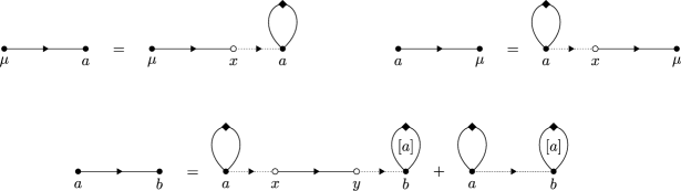
Figure 9.1: The graphical representation of the rules (8.4) (using $a$ and $b$ for summation indices and $\mu$ for external index instead of the generic indices $u$ and $v$). Two of the loops on the last line correspond to resolvent entries $G_{bb}^{(\bm{\mathrm{a}}\setminus\{a,b\})}$ which are not maximally expanded: they still depend on $a$, which is indicated by the label $[a]$ inside the loop.

The term $A^{\prime\prime}$ from Step 3 arises from taking the second term on the right-hand sides of (9.3), which in the graphical language translates to creating two (non-loop) resolvent edges connecting the vertices $i$ and $j$ associated with the indices $u$ and $v$ respectively, i.e. linking a loop at $i$ with $j$. We call this process linking $i$ with $j$. See Figure 9.2.

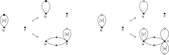
Figure 9.2: Linking the vertex $i$ (depicted in the picture with its associated index $u$) with the vertex $j$ (depicted with index $v$). These two diagrams correspond to the two identities in (9.3). As in Figure 9.1, if a diagonal resolvent entry encoded by a loop is not maximally expanded, we indicate the index on which it depends in angular brackets inside the loop.

This graphical algorithm provides an alternative, graphical, construction of $\mathfrak{D}(\Gamma)$ starting from $\Gamma$. Each $\Pi\in\mathfrak{D}(\Gamma)$ encodes a monomial $\mathcal{A}(\Pi)$ whose resolvent entries satisfy ($*$). As in Section 8, the vertex set of $\Pi$ may be written as $V(\Pi)=V_{f}(\Pi)\sqcup V_{s}(\Pi)\sqcup V_{e}(\Pi)$, corresponding to the fresh summation vertices, the original summation vertices, and the external vertices, respectively. Note that $\Pi$ now contains loops, which bear either a black or white diamond (encoding diagonal entries of $G$ in the numerator or denominator respectively). Moreover, each diagonal entry encoded by a loop of $\Pi$ is maximally expanded, and each off-diagonal entry encoded by a non-loop edge of $\Pi$ has upper indices $\bm{\mathrm{a}}$. See Figure 9.3 for a simple example of the process $\Gamma\mapsto\Pi\in\mathfrak{D}(\Gamma)$.

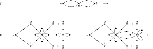
Figure 9.3: The process $\Gamma\mapsto\Pi\in\mathfrak{D}(\Gamma)$, where we draw the two simplest elements of $\mathfrak{D}(\Gamma)$ on the bottom line. (For reasons of space, we omit the labels $a$ and $b$ on the bottom line.) The first graph is just the top-middle graph of Figure 8.5 but with added loops. In the second graph one loop at $a$ was linked with $b$.

9.1.2. Generation of the fresh summation vertices (revisited), Step II: from $\Pi$ to $\Theta$

In this section we complete the second part of the generation of the fresh summation vertices, by constructing a family of graphs $\Theta\in\mathfrak{R}(\Pi)$ from $\Pi$. The underlying algebraic identity is (9.2).

Lemma 9.3.

For any $K\in\mathbb{N}$ and any $\Pi\in\mathfrak{D}(\Gamma)$ there is a decomposition

$$\mathcal{A}(\Pi)\;=\;\sum_{\alpha}B_{\alpha}+O_{\prec}(\Psi^{K})\,,$$ (9.6)

such that each $B_{\alpha}$ is a monomial in the entries of $G^{(\bm{\mathrm{a}})}$ and the $\bm{\mathrm{a}}$-admissible entries of $H$. The sum over $\alpha$ ranges over a finite set that is independent of $N$.

We shall apply Lemma 9.3 with the choice $K\mathrel{\vbox{\hbox{.}\hbox{.}}}=p(\deg(\Delta)+2\lvert V_{s}(\Delta)\rvert)$, which will ensure that the error term $O_{\prec}(\Psi^{K})$ is negligible.

Proof of Lemma 9.3.

We simply apply (9.2) to each diagonal resolvent entry of $\mathcal{A}(\Pi)$. Recall that each diagonal resolvent entry of $\mathcal{A}(\Pi)$ is maximally expanded, which implies that all resolvent entries explicitly appearing in the definition (3.15) for $Z_{a}^{(\bm{\mathrm{a}}\setminus\{a\})}$ and $U_{a}^{(\bm{\mathrm{a}})}$ have upper indices $\bm{\mathrm{a}}$. Then, as above, it immediately follows that if we pick the rest term $O_{\prec}(\Psi^{K})$ in (9.2) from any diagonal entry, the resulting monomial is $O_{\prec}(K)$ and may be absorbed into the error term on the right-hand side of (9.6).

For the following we therefore assume that there are no rest terms $O_{\prec}(\Psi^{K})$ in the expansion (9.2) of the diagonal resolvent entries of $\mathcal{A}(\Pi)$. The result is a finite family of monomials whose number does not depend on $N$ (but does of course depend on $K$), and which may again be represented graphically. In such graphs we represent a term $U_{a}^{(\bm{\mathrm{a}})}$ with a solid ring around the vertex associated with $a$ (these terms $U_{a}^{(\bm{\mathrm{a}})}$ will not be expanded further, so their precise structure does not matter; the number of rings simply encode their size). See Figure 9.4 for a depiction of the three nontrivial terms arising from the expansion of $G_{aa}^{(\bm{\mathrm{a}}\setminus\{a\})}$.

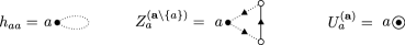
Figure 9.4: The graphical representation of the three error terms resulting from the expansion of $G_{aa}^{(\bm{\mathrm{a}}\setminus\{a\})}$ using (9.2). Apart from the entries of $H$ encoded by the dotted edges, all terms are independent of $\bm{\mathrm{a}}$.

Thus, when expanding a loop at $a$ with a white diamond (encoding $1/G_{aa}^{(\bm{\mathrm{a}}\setminus\{a\})}$), we replace the loop with either nothing (corresponding to the term $1/m$ used in the argument of Section 8) or one of the three pieces in Figure 9.4. Similarly, when expanding a loop at $a$ with a black diamond (encoding $G_{aa}^{(\bm{\mathrm{a}}\setminus\{a\})}$), we replace the loop with either nothing (corresponding to a factor $m$ coming from the zeroth order term in the summation in (9.2)) or an agglomeration of pieces from Figure 9.4 at the vertex associated with $a$. (We use concentric rings around $a$ to depict several factors $U_{a}^{(\bm{\mathrm{a}})}$). See Figure 9.5.

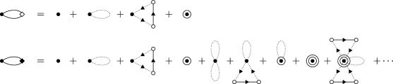
Figure 9.5: Expanding a loop. The two lines correspond to the two identities of (9.2) respectively.

The application of (9.2) to the diagonal entries encoded by $\Pi$ yields a new family of graphs, which we call $\mathfrak{R}(\Pi)$ and whose elements we denote by $\Theta$. Each resolvent edge of $\Theta\in\mathfrak{R}(\Pi)$ now encodes an entry of $G^{(\bm{\mathrm{a}})}$ or $G^{(\bm{\mathrm{a}})*}$. We also have the usual self-explanatory splitting $V(\Theta)=V_{f}(\Theta)\sqcup V_{s}(\Theta)\sqcup V_{e}(\Theta)$. See Figure 9.6 for an example of the process $\Pi\mapsto\mathfrak{R}(\Pi)$.

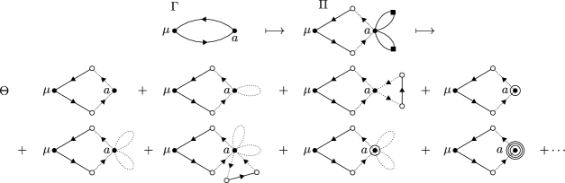
Figure 9.6: The process $\Gamma\mapsto\Pi\mapsto\Theta$. On the second line we draw four graphs $\Theta$ corresponding to choosing one of the four terms on the right-hand side of the first equation of (9.2). On the third line we draw some more complicated graphs $\Theta$.

∎

Summarizing the results of this Sections 9.1.1 and 9.1.2, for a given $\Gamma\in\mathfrak{G}_{F}^{p}(\Delta)$, we have constructed an $N$-independent set of graphs,

$$\mathfrak{R}(\mathfrak{D}(\Gamma))\;=\;\bigcup\bigl{\{}{\mathfrak{R}(\Pi)\mathrel{\vbox{\hbox{.}\hbox{.}}}\Pi\in\mathfrak{D}(\Gamma)}\bigr{\}}\,.$$

If $\Theta\in\mathfrak{R}(\mathfrak{D}(\Gamma))$ then each resolvent entry of $\mathcal{A}(\Theta)$ has upper indices $\bm{\mathrm{a}}$, and the fresh summation indices $\bm{\mathrm{x}}=(x_{i})_{i\in V_{f}(\Theta)}$ and the original summation indices $\bm{\mathrm{a}}=(a_{i})_{i\in V_{s}(\Theta)}$ are disjoint. Moreover, we have the splitting

$$\mathcal{A}_{\bm{\mathrm{a}}}(\Gamma)\;=\;\sum_{\Theta\in\mathfrak{R}(\mathfrak{D}(\Gamma))}\sum_{\bm{\mathrm{x}}}^{(\bm{\mathrm{a}})}\mathcal{A}_{\bm{\mathrm{a}},\bm{\mathrm{x}}}(\Theta)+O_{\prec}\bigl{(}{\Psi^{p(\deg(\Delta)+2\lvert V_{s}(\Delta)\rvert)}}\bigr{)}$$

where we explicitly indicated the set of summation indices in the subscript of $\mathcal{A}$, see (8.3). Note that the elements of the family $\mathfrak{R}(\mathfrak{D}(\Gamma))$ have the same properties as the elements of the smaller set $\widetilde{\mathfrak{R}}(\Gamma)$ from Section 8.

9.1.3. Lumping of the fresh summation vertices (revisited) and conclusion of the estimate

Fix a $\Theta\in\mathfrak{R}(\mathfrak{D}(\Gamma))$. Now we may proceed as in Section 8.3 and take the lumping of the entries of $H$ in $\mathcal{A}(\Theta)$ by computing their partial expectation $\prod_{a\in\bm{\mathrm{a}}}P_{a}$. Since all resolvent entries of $\mathcal{A}(\Theta)$ are independent of $\bm{\mathrm{a}}$, this partial expectation acts only on the entries of $H$, and leads to lumpings exactly as in Section 8.3. This gives rise to a family of graphs $\Upsilon\in\mathfrak{L}(\Theta)$. As before, we seek to gain a factor $\Phi$ from each marked vertex $i\in V_{m}(\Gamma)$.

Thus, let us fix a sequence $\Gamma\mapsto\Pi\mapsto\Theta\mapsto\Upsilon$. It is convenient to extend the definition of the degree of a vertex as follows. By definition, the degree of $i\in V(\Theta)$, written $\deg_{\Theta}(i)$, is equal to the number of legs incident to $i$ plus two times the number of rings around $i$. This convention is chosen so that each error term in Figure 9.4 increases the degree of $i$ by two.

Now take a marked vertex $i\in V_{m}(\Gamma)$. Note that, by construction of $\Pi$ and $\Theta$, we have $\deg_{\Theta}(i)\geqslant\deg_{\Gamma}(i)$. We consider two cases.

1. Suppose that $\deg_{\Theta}(i)=\deg_{\Gamma}(i)$. This means that in the process $\Gamma\mapsto\Pi$ the original summation vertex $i$ was not linked with another original summation vertex (see Section 9.1.1), and that in the process $\Pi\mapsto\Theta$ (see Section 9.1.2) we always chose the main term ($1/m$ or $m$) on the right-hand sides of (9.2) when applying (9.2) to any diagonal entries with lower indices $a_{i}a_{i}$. In particular, (8.10) holds. We may therefore proceed exactly as in Section 8: any pairing in $\Theta\mapsto\Upsilon$ of the white vertices adjacent to $i$ gives rise to at least one chain vertex of $\Upsilon$ (see Definition 8.6). A higher-order lumping (i.e. one that is not a pairing) gives rise to a positive power of $M^{-1/2}\leqslant\Psi$. Either way, we shall gain a factor $\Phi$ from $i$ after summing over $\bm{\mathrm{x}}$ and invoking Proposition 5.3.

2. Suppose that $\deg_{\Theta}(i)>\deg_{\Gamma}(i)$. In this case we have that either

   1. in the process $\Gamma\mapsto\Pi$ the vertex $i$ was linked to another original summation vertex, or

   2. in the process $\Pi\mapsto\Theta$ we chose at least one error term (represented graphically by one of the graphs in Figure 9.4) on the right-hand sides of (9.2) when applying (9.2) to the diagonal entries with lower indices $i$.

   We claim that either case, (ii.1) or (ii.2), results in an extra error factor in $\Upsilon$ of order $\Psi$.

   In order to see this, consider first the case (ii.1). Here the linking means that there is a $j\in V_{s}(\Upsilon)$ such that in $\Upsilon$ we have two extra resolvent edges (as compared to case (i)), each connecting a vertex in $p^{-1}(i)$ to a vertex in $p^{-1}(j)$. This yields a factor $\Psi^{2}$. Thus we gain a factor $\Psi$ that we ascribe to $i$ (the other factor $\Psi$ is in general not available, as it may be needed for exactly the same reason at the vertex $j$). Next, consider the case (ii.2). If there is a term $h_{aa}$ or $U_{a}^{(\bm{\mathrm{a}})}$ in $\mathcal{A}(\Theta)$, then we immediately get a factor $\Psi\Phi$. (For $U_{a}^{(\bm{\mathrm{a}})}$ this is trivial by (9.1) and for $h_{aa}$ taking $P_{a}$ implies that there must be at least another factor $h_{aa}$, in which case we get a factor $M^{-1}\leqslant\Psi\Phi$.) Finally, if we have a factor $Z_{a}^{(\bm{\mathrm{a}}\setminus\{a\})}$ observe that in the expression

   $$Z_{a}^{(\bm{\mathrm{a}}\setminus\{a\})}\;=\;Q_{a}\Biggl{(}{\sum_{x,y}^{(\bm{\mathrm{a}})}h_{ax}G_{xy}^{(\bm{\mathrm{a}})}h_{ya}}\Biggr{)}$$ (9.7)

   we cannot pair $h_{ax}$ with $h_{ya}$ when computing the partial expectation $P_{a}$ (since $P_{a}Q_{a}=0$). (Of course in a higher-order lumping, they could be in the same lump provided this lump contains at least three elements.) This implies that, in the leading-order pairing, the fresh summation vertices of $\Theta$ associated with $x$ and $y$ will be paired into different vertices of $\Upsilon$. In particular, we gain an additional off-diagonal resolvent entry $G_{xy}^{(\bm{\mathrm{a}})}\prec\Psi$. See Figure 9.7 for a graphical depiction of this lumping.

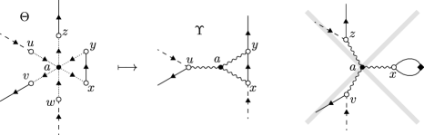
Figure 9.7: The lumping of fresh summation vertices in the presence of a factor $Z_{a}^{(\bm{\mathrm{a}}\setminus\{a\})}$ (represented by a triangle in $\Theta$.). Due to the $Q_{a}$ in the definition of $Z_{a}^{(\bm{\mathrm{a}}\setminus\{a\})}$, the last graph (crossed out in grey) does not contribute.

In summary, each marked vertex $i$ therefore yields a gain of $\Phi$ upon summation over $\bm{\mathrm{x}}$. This concludes the proof of Theorem 4.8 without Simplification (S3).

9.2.  Removing Simplification (S2)

In this section we revisit the arguments of Sections 8 and 9.1, and explain the modifications required if we relax Simplification (S2), i.e. allow diagonal entries $\mathcal{G}_{aa}=G_{aa}-m$ in the definition of $\mathcal{Z}$. (On the level of $\Delta$, this amounts to allowing loops.) The construction of $\Gamma\in\mathfrak{G}_{F}^{p}(\Delta)$ remains unchanged. Each diagonal entry of $\mathcal{A}(\Gamma)$ is maximally expanded, i.e. of the form $\mathcal{G}_{aa}^{(\bm{\mathrm{a}}\setminus\{a\})}$. Hence the construction of $\Pi\in\mathfrak{D}(\Gamma)$ from $\Gamma$ carries over unchanged from Section 9.1.1. Now $\Pi$ has loops of three kinds: with a black diamond (encoding $G_{aa}^{(\bm{\mathrm{a}}\setminus\{a\})}$), with a white diamond (encoding $1/G_{aa}^{(\bm{\mathrm{a}}\setminus\{a\})}$), and plain (encoding $\mathcal{G}_{aa}^{(\bm{\mathrm{a}}\setminus\{a\})}$). Note that a decorated loop encodes a factor of size $O_{\prec}(1)$ while a plain loop encodes a factor of size $O_{\prec}(\Psi)$. The additional difficulty in this section as compared to Section 8 is that the naive size of a plain loop is smaller than the size of the decorated loops dealt with in Section 8. Thus we have to establish bounds which, in addition to the gain extracted in Section 8, also contain the smallness associated with the naive size of a plain loop.

The process $\Pi\mapsto\Theta\in\mathfrak{R}(\Pi)$, in which all (maximally expanded) diagonal entries are expanded using (9.2) is again the same as that of Section 9.1.2. For $1/G_{aa}^{(\bm{\mathrm{a}}\setminus\{a\})}$ and $G_{aa}^{(\bm{\mathrm{a}}\setminus\{a\})}$ we use (9.2), and, in addition, for $\mathcal{G}_{aa}^{(\bm{\mathrm{a}}\setminus\{a\})}$ we use

$$\mathcal{G}_{aa}^{(\bm{\mathrm{a}}\setminus\{a\})}\;=\;\sum_{k=1}^{K-1}m^{k+1}\bigl{(}{-h_{aa}+Z_{a}^{(\bm{\mathrm{a}}\setminus\{a\})}+U_{a}^{(\bm{\mathrm{a}})}}\bigr{)}^{k}+O_{\prec}(\Psi^{K})$$ (9.8)

(note that the sum starts with $k=1$). Finally, lumping the white summation vertices yields the graph $\Upsilon$. As in Section 9.1.3, the important observation is that the two white vertices associated with a $Z_{a}^{(\bm{\mathrm{a}}\setminus\{a\})}$ (see Figure 9.4) cannot be paired. In summary, the resolution process $\Gamma\mapsto\Pi\mapsto\Theta\mapsto\Upsilon$ is almost identical to that in Sections 8 and 9.1. There is only one new ingredient: the expansion (9.8) which starts with $k=1$.

To illustrate this procedure, let us consider the simple example with $\bm{\mathrm{a}}=\{a\}$

$$\mathbb{E}G_{\mu a}^{*}G_{a\mu}\mathcal{G}_{aa} \;=\;\mathbb{E}\sum_{x,y}^{(a)}G_{aa}G_{aa}^{*}h_{ax}G_{x\mu}^{(a)}G_{\mu y}^{(a)*}h_{ya}\mathcal{G}_{aa}$$

$$\;=\;m^{2}\bar{m}\,\mathbb{E}\sum_{x,y}^{(a)}h_{ax}G_{x\mu}^{(a)}G_{\mu y}^{(a)*}h_{ya}\biggl{(}{Q_{a}\sum_{z,w}^{(a)}h_{az}G_{zw}^{(a)}h_{wa}-h_{aa}+U_{a}^{(a)}}\biggr{)}+\cdots$$

$$\;=\;m^{2}\bar{m}\,\mathbb{E}\sum_{x,y}^{(a)}s_{ax}s_{ay}G_{\mu y}^{(a)*}G_{yx}^{(a)}G_{x\mu}^{(a)}+0+m^{2}\bar{m}\,\mathbb{E}\sum_{x}s_{ax}G_{\mu x}^{(a)*}G_{x\mu}^{(a)}U_{a}^{(a)}+\cdots\,,$$ (9.9)

where $+\cdots$ denotes higher-order terms in the expansion (9.2) and (9.8). The expectation of the middle term in the parentheses vanishes because $\mathbb{E}h_{aa}=0$. See Figure 9.8 for a graphical version of (9.9).

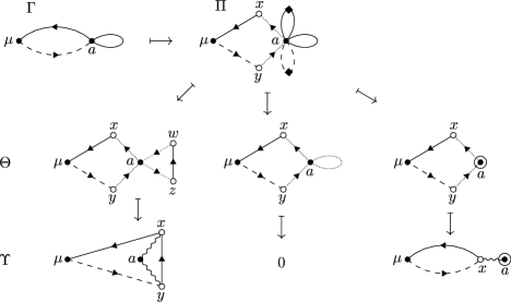
Figure 9.8: The complete resolution process $\Gamma\mapsto\Pi\mapsto\Theta\mapsto\Upsilon$ for the example (9.9). At each step we only draw the leading-order graphs. The first, second, and third lines of the figure correspond to the first, second, and third lines of (9.9) respectively.

Note that each unmarked loop (encoding a diagonal entry of $\mathcal{G}$) contributes a factor $O_{\prec}(\Psi)$ to $\mathcal{A}(\Gamma)$. When performing the vertex resolution $\Gamma\mapsto\Upsilon$, we therefore have to ensure that this gain of $\Psi$ is not lost (i.e. that $\mathcal{A}(\Upsilon)$ has an associated factor of size $O_{\prec}(\Psi)$). In addition, we have to gain a factor $\Phi$ from each marked vertex of $\Upsilon$.

In the example (9.9), the vertex $a$ is marked and each term on the bottom line of (9.9) is of order $\Psi^{3}\Phi$. This bound should be read as $\Psi^{2}\Psi\Phi$, where $\Psi^{2}$ is the trivial bound on the off-diagonal entries, $\Psi$ is the bound on the diagonal entry of $\mathcal{G}$, and $\Phi$ is the additional gain arising from the fact that $a$ is marked. Indeed, the first term on the bottom line of (9.9) is of order $\Psi^{3}\Phi$ by Proposition 5.3, and the last term of order $\Psi^{4}$ by Lemma 9.1.

This is in fact a general phenomenon. Let $i\in V_{m}(\Gamma)$ be marked, with associated summation index $a$. We shall give the details only for a leading-order graph $\Upsilon$, i.e.  a graph $\Upsilon$ that satisfies:

1. In the process $\Gamma\mapsto\Pi$ the original summation vertex $i$ was not linked with another original summation vertex.

2. In the process $\Pi\mapsto\Theta$ we always chose the main term ($1/m$ or $m$) on the right-hand sides (9.2), and the term $mZ_{a}^{(\bm{\mathrm{a}}\setminus\{a\})}$ on the right-hand side of (9.8).

3. In the process $\Theta\mapsto\Upsilon$, we chose a pairing of the white vertices incident to $i$. (I.e. no higher-order lumping is allowed.)

If $\Upsilon$ does not satisfy (i) – (iii), an argument almost identical to that of Sections 8.4 and 9.1.3 yields an extra factor $\Phi$, in addition to $\Psi^{\ell}$ where $\ell$ is the number of plain loops incident to $i$ in $\Gamma$. (This is a simple power counting that uses the fact that each $U_{a}^{({\bf{a}})}$ yields a factor $\Psi\Phi$, and each $h_{aa}$ and $Z_{a}^{(\bm{\mathrm{a}}\setminus\{a\})}$ yield a factor $\Psi$ each. That $Z_{a}^{(\bm{\mathrm{a}}\setminus\{a\})}$ yields a factor $\Psi$ follows from the observation that after resolution it yields an off-diagonal resolvent entry in $\mathcal{A}(\Upsilon)$, as explained after (9.7). Note that, unlike in Section 9.1.3 where it was enough to gain a factor $\Psi$ from $U_{a}^{(\bm{\mathrm{a}})}$, here it is crucial that $U_{a}^{(\bm{\mathrm{a}})}\prec\Psi\Phi$.)

Let us therefore assume that $\Upsilon$ satisfies (i) – (iii). By (i) and (ii) we have (8.10). Recall the definition of the projection $p$ from (iv) in Section 8.3. Each $j\in p^{-1}(i)$ is incident to precisely two resolvent edges and one wiggly edge that is also incident to $i$. Moreover, no vertex of $p^{-1}(i)$ is incident to a loop; this follows from the above observation that the two white vertices associated with $mZ_{a}^{(\bm{\mathrm{a}}\setminus\{a\})}$ cannot be paired. From (8.2) and (8.10), we therefore find that at least one vertex in $p^{-1}(i)$ is a chain vertex. Consequently summation over $\bm{\mathrm{x}}$ results in an extra factor $\Phi$ by Proposition 5.3, and hence completes the argument.

9.3.  Removing Simplification (S4)

In this section we remove Simplification (S4), by allowing the fresh summation indices $\bm{\mathrm{x}}$ to coincide with each other and with external indices $\bm{\mathrm{\mu}}$. This entails proving Proposition 5.3 without the simplifying assumption (S4) that was assumed in its proof. Roughly, there are two kinds of problems arising from such coincidences: an off-diagonal resolvent entry $G_{xy}$ may become diagonal (hence leading to a loss of a factor $\Psi$), and a chain vertex may cease to be one (hence leading to a loss of a factor $\Phi$). However, these losses are compensated by powers of $M^{-1}$ resulting from a reduction in the number of independent summation variables. The main point is to prove each coincidence of summation variables results in a loss of at most two factors of $\Psi$ and at most two factors of $\Phi$. Since $M^{-1}\leqslant\Psi^{2}\Phi^{2}$, the gain of $M^{-1}$ will be enough to compensate this loss.

Throughout Sections 8, 9.1, and 9.2, we invoked Proposition 5.3 in order to gain from chain vertices. To that end, we had to assume Simplification (S4) (since the indices $(\bm{\mathrm{x}},\bm{\mathrm{\mu}})$ are assumed to be disjoint in Proposition 5.3). The main result of this section is the following extension of Proposition 5.3. It states that the stochastic bound of Proposition 5.3 is valid even if the summation over $\bm{\mathrm{x}}$ has no restriction. (As in Proposition 5.3, we use $\bm{\mathrm{a}}$ to denote the summation indices; in our applications of Proposition 9.4 $\bm{\mathrm{a}}$ always consists of fresh summation vertices which we denoted by $\bm{\mathrm{x}}$ in Sections 8, 9.1, and 9.2.)

Proposition 9.4.

Suppose that $\Lambda\prec\Psi$ for some admissible control parameter $\Psi$. Let $\Delta$ be a chain encoding $\mathcal{Z}_{\bm{\mathrm{a}}}$. Then

$$\sum_{\bm{\mathrm{a}}}w(\bm{\mathrm{a}})\mathcal{Z}_{\bm{\mathrm{a}}}\;\prec\;\Psi^{\deg(\Delta)}\Phi^{c(\Delta)}$$ (9.10)

for any $\bm{\mathrm{\mu}}$ and chain weight $w$.

Proof.

The basic idea is to split the summation into partitions

$$\sum_{\bm{\mathrm{a}}}w(\bm{\mathrm{a}})\mathcal{Z}_{\bm{\mathrm{a}}}\;=\;\sum_{P}\sum_{\bm{\mathrm{a}}}\bm{\mathrm{1}}\bigl{(}{\mathcal{P}(\bm{\mathrm{\mu}},\bm{\mathrm{a}})=P}\bigr{)}w(\bm{\mathrm{a}})\mathcal{Z}_{\bm{\mathrm{a}}}\,,$$

where $P$ ranges over all partitions of $V(\Delta)$, and $\mathcal{P}$ was introduced in Definition 4.3. Note that, since $\bm{\mathrm{\mu}}$ are constrained to be distinct, if $P$ yields a nonzero contribution each of its blocks may contain at most one vertex in $V_{e}(\Delta)$. For the following we fix a partition $P$ and prove that

$$\mathcal{X}_{P}\;\mathrel{\vbox{\hbox{.}\hbox{.}}}=\;\sum_{\bm{\mathrm{a}}}\bm{\mathrm{1}}\bigl{(}{\mathcal{P}(\bm{\mathrm{\mu}},\bm{\mathrm{a}})=P}\bigr{)}w(\bm{\mathrm{a}})\mathcal{Z}_{\bm{\mathrm{a}}}$$

is stochastically bounded by the right-hand side of (9.10). On the level of the graph $\Delta$, a nontrivial partition $P$ of $V(\Delta)$ results in a merging of vertices $V(\Delta)$. By merging vertices of $\Delta$ we therefore get a new graph which we denote by $P(\Delta)$. The vertex set of $P(\Delta)$ has the usual decomposition $V(P(\Delta))=V_{e}(P(\Delta))\sqcup V_{s}(P(\Delta))$, where $V_{e}(P(\Delta))=V_{e}(\Delta)$ and $V_{s}(P(\Delta))$ is given by the set of blocks of $P$ that do not contain a vertex from $V_{e}(\Delta)$. A vertex $i\in V(P(\Delta))$ is unmerged if the corresponding block has size one, and merged otherwise. See Figure 9.9 for an example of the merging $\Delta\mapsto P(\Delta)$.

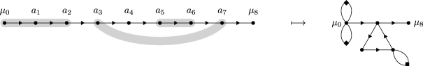
Figure 9.9: The merging $\Delta\mapsto P(\Delta)$ of summation vertices of a chain. The vertices of $\Delta$ are $V_{s}(\Delta)=\{1,\dots,7\}$ and $V_{e}(\Delta)=\{0,8\}$. We chose the partition $P=\{{\{0,1,2\},\{3,7\},\{4\},\{5,6\},\{8\}}\}$.

For concreteness assume first that $\Delta$ is an open chain with $V(\Delta)=\{0,\dots,n\}$, where $V_{e}(\Delta)=\{0,n\}$. Thus, $\deg(\Delta)=n$. For any graph $\Delta^{\prime}$ define the set of vertices

$$V_{g}(\Delta^{\prime})\;\mathrel{\vbox{\hbox{.}\hbox{.}}}=\;\bigl{\{}{i\in V_{s}(\Delta^{\prime})\mathrel{\vbox{\hbox{.}\hbox{.}}}\text{$i$ has degree two without counting loops}}\bigr{\}}\,.$$

Thus, the set $V_{g}(P(\Delta))$ includes not only the chain vertices of $P(\Delta)$ but also chain vertices to which one more loops are attached. Let $r(\Delta^{\prime})$ denote the number of edges of $\Delta^{\prime}$ that are not loops, and set $c(\Delta^{\prime})\mathrel{\vbox{\hbox{.}\hbox{.}}}=\lvert V_{g}(\Delta^{\prime})\rvert$. In particular, if $\Delta^{\prime}$ is a chain then this definition agrees with that from Definition 5.1. (For example, in Figure 9.9 we have $c(P(\Delta))=2$ and $r(P(\Delta))=5$.)

Define $k\mathrel{\vbox{\hbox{.}\hbox{.}}}=n-1-\lvert V_{s}(P(\Delta))\rvert$. Informally, $k$ is the number of summation vertices of $V_{s}(\Delta)$ that have been merged into some other vertex. As we shall see, $k$ is the exponent of $M^{-1}$ which describes the reduction in the combinatorics of the summation. (In Figure 9.9 we have $n=8$ and $\lvert V_{s}(P(\Delta))\rvert=3$, which gives $k=4$.) We claim that

$$n-k\;\leqslant\;r(P(\Delta))\;\leqslant\;n\,,\qquad r(P(\Delta))+c(P(\Delta))\;\geqslant\;2n-1-2k\,.$$ (9.11)

The easiest way to prove (9.11) is by the following inductive argument. We construct $P(\Delta)$ from $\Delta$ by successively merging one vertex at a time, and follow the change of the functions $r(\cdot)$ and $r(\cdot)+c(\cdot)$ at each step. The formal procedure is the following. We construct a sequence of graphs $\Delta_{0}=\Delta,\Delta_{1},\dots,\Delta_{k}=P(\Delta)$ as follows. We start from $\Delta_{0}\mathrel{\vbox{\hbox{.}\hbox{.}}}=\Delta$. Recall that the vertices of $\Delta$ are naturally ordered by $\leqslant$. Let $i_{1}\in V_{s}(\Delta)$ be the smallest vertex of $\Delta$ that is in a nontrivial block (i.e. of size greater than one) of $P$. Set $\Delta_{1}$ to be the graph obtained from $\Delta_{0}$ by merging $i_{1}$ with the (unique) vertex $j\in V(\Delta_{0})$ satisfying $j<i_{1}$. The vertices of $\Delta_{1}$ remain ordered after we assign the newly created merged vertex the index $j$. Similarly, $\Delta_{l+1}$ is obtained from $\Delta_{l}$ by choosing the smallest unmerged vertex $i_{l}\in V_{s}(\Delta_{l})$ that is in a nontrivial block of $P$, and merging it with the unique $j\in V(\Delta_{l})$ satisfying $j<i_{l}$. After $k$ steps of this procedure, we obtain $\Delta_{k}=P(\Delta)$. Moreover, it is easy to see for $0\leqslant l\leqslant k-1$ that

$$r(\Delta_{l})-1\;\leqslant\;r(\Delta_{l+1})\;\leqslant\;r(\Delta_{l})\,,\qquad r(\Delta_{l+1})+c(\Delta_{l+1})\;\geqslant\;r(\Delta_{l})+c(\Delta_{l})-2\,.$$ (9.12)

Indeed, either $i_{l}$ is merged with a vertex adjacent to itself, in which case we have $r(\Delta_{l+1})=r(\Delta_{l})-1$ and $c(\Delta_{l+1})\geqslant c(\Delta_{l})-1$, or $i_{l}$ is merged with a vertex not adjacent to itself, in which case we have $r(\Delta_{l+1})=r(\Delta_{l})$ and $c(\Delta_{l+1})\geqslant c(\Delta_{l})-2$. Since $r(\Delta)+c(\Delta)=2n-1$, (9.11) follows from (9.12).

We may now sum over $(a_{i})_{i\in V_{s}(P(\Delta))}$. To that end, if $i\in V_{g}(P(\Delta))$ and there is a loop (or several loops) at $i$, then we expand each corresponding diagonal term $G_{a_{i}a_{i}}$ as $G_{a_{i}a_{i}}=m+(G_{a_{i}a_{i}}-m)$. If we pick a factor $m$ from each loop, $i$ becomes a chain vertex. If we pick at least one factor $G_{a_{i}a_{i}}-m$, $i$ is not a chain vertex but carries a factor of order $\Psi$. Either way, summing over $a_{i}$ yields a factor $\Phi$ by Proposition 5.3. (Note that Proposition 5.3 is applicable to the graph $P(\Delta)$ because all summation indices are constrained to be distinct.) Thus we get the bound

$$\mathcal{X}_{P}\;\prec\;M^{-k}\Psi^{r(P(\Delta))}\Phi^{c(P(\Delta))}\;\leqslant\;M^{-k}\Psi^{n-k}\Phi^{n-1-2k}\,,$$

where in the last step we used (9.11). Since $M^{-1}\Psi^{-1}\Phi^{-2}\leqslant\Psi\leqslant 1$ we find $\mathcal{X}_{P}\prec\Psi^{n}\Phi^{n-1}$, which is (9.10).

The case of a closed chain $\Delta$ of degree $n$ is handled similarly. For definiteness assume that $\Delta$ has no external vertex. Now we have $k\mathrel{\vbox{\hbox{.}\hbox{.}}}=n-\lvert V_{s}(P(\Delta))\rvert\leqslant n-1$ and we let $l$ range from $0$ to $k$. Then (9.12) holds for $l=0,\dots,n-3$. If $l=n-2$ then (9.12) is in general false (as can be seen e.g. on the open chain of degree two with $V_{s}(\Delta)=\{1,2\}$ and $P=\{\{1,2\}\}$). In that case we replace it with the trivial bounds $r(\Delta_{n-1})\geqslant 0$ and $c(\Delta_{n-1})\geqslant 0$. Thus if $k\leqslant n-2$ then we find (9.10) exactly as above, and if $k=n-1$ we get using $n\geqslant 2$

$$\mathcal{X}_{P}\;\prec\;M^{-k}\Psi^{r(P(\Delta))}\Phi^{c(P(\Delta))}\;\leqslant\;M^{-n+1}\;\leqslant\;\Psi^{n}\Phi^{n}\,,$$

which is (9.10). ∎

To conclude this section, we address an issue concerning coinciding indices that was repeatedly swept under the rug in Sections 7, 8, 9.1, and 9.2. Essentially, we do an inclusion-exclusion argument on the values of the summation indices of a union of chains so as to decouple the summations associated with different subchains. Recall the definition of $X_{F}^{w}(\Delta)$ from (4.5).

Lemma 9.5.

If $\Delta=\Delta_{1}\cup\cdots\cup\Delta_{k}$ is a union of chains then

$$X^{w}_{\emptyset}(\Delta)\;\prec\;\prod_{l=1}^{k}\Psi^{\deg(\Delta_{l})}\Phi^{c(\Delta_{l})}\,.$$ (9.13)

In words: if $\Delta$ is a union of chains, then in the summation over $\bm{\mathrm{a}}$ in $X^{w}_{\emptyset}(\Delta)$ we can decouple the summations associated with different subchains of $\Delta$. (In $X^{w}_{\emptyset}(\Delta)$ these summations are coupled by the constraint that indices associated with different subchains are distinct.)

Proof of Lemma 9.5.

This is a simple decoupling of the summation indices. Let $\bm{\mathrm{a}}^{l}$ and $\bm{\mathrm{\mu}}^{l}$ denote the summation and external indices of $\Delta_{l}$. Abbreviate $\mathcal{Z}_{\bm{\mathrm{a}}^{l}}^{\bm{\mathrm{\mu}}^{l}}(\Delta_{l})\equiv\mathcal{Z}^{l}_{\bm{\mathrm{a}}^{l}}$. Thus we have

$$X_{\emptyset}(\Delta)\;=\;\sum_{\bm{\mathrm{a}}^{1}\cdots\bm{\mathrm{a}}^{k}}^{(\bm{\mathrm{\mu}}^{1}\cdots\bm{\mathrm{\mu}}^{k})*}w(\bm{\mathrm{a}}^{1},\dots,\bm{\mathrm{a}}^{k})\mathcal{Z}^{1}_{\bm{\mathrm{a}}^{1}}\cdots\mathcal{Z}^{k}_{\bm{\mathrm{a}}^{k}}\;=\;\sum_{\bm{\mathrm{a}}^{1}\cdots\bm{\mathrm{a}}^{k}}I(\bm{\mathrm{a}}^{1},\dots,\bm{\mathrm{a}}^{k})\,w(\bm{\mathrm{a}}^{1},\dots,\bm{\mathrm{a}}^{k})\mathcal{Z}^{1}_{\bm{\mathrm{a}}^{1}}\cdots\mathcal{Z}^{k}_{\bm{\mathrm{a}}^{k}}\,,$$

where the indicator function $I$ explicitly enforces that all $a_{i}^{l}$’s are distinct from all $\mu_{i}^{l}$’s and they are district among themselves. Explicitly,

$$I(\bm{\mathrm{a}}^{1},\dots,\bm{\mathrm{a}}^{k})\;\mathrel{\vbox{\hbox{.}\hbox{.}}}=\;\Biggl{[}{\prod_{l=1}^{k}\prod_{i,j\in V_{s}(\Delta_{l})}^{*}\bigl{(}{1-\bm{\mathrm{1}}(a_{i}^{l}=a_{j}^{l})}\bigr{)}}\Biggr{]}\Biggl{[}{\prod_{l,m\leqslant k}\prod_{i\in V_{s}(\Delta_{l})}\prod_{j\in V_{e}(\Delta_{m})}\bigl{(}{1-\bm{\mathrm{1}}(a_{i}^{l}=\mu_{j}^{m})}\bigr{)}}\Biggr{]}\\ \times\Biggl{[}{\prod_{l,m\leqslant k}^{*}\prod_{i\in V_{s}(\Delta_{l})}\prod_{j\in V_{s}(\Delta_{m})}\bigl{(}{1-\bm{\mathrm{1}}(a_{i}^{l}=a_{j}^{m})}\bigr{)}}\Biggr{]}\,.$$

Multiplying out each parenthesis in the definition of $I$, we get a splitting of the form $I=\sum_{\alpha}I_{\alpha}$ (the sum ranges over a finite set which depends only on $\Delta$). For each $\alpha$, we may now estimate

$$\sum_{\bm{\mathrm{a}}^{1}\cdots\bm{\mathrm{a}}^{k}}I_{\alpha}(\bm{\mathrm{a}}^{1},\dots,\bm{\mathrm{a}}^{k})\,w(\bm{\mathrm{a}}^{1},\dots,\bm{\mathrm{a}}^{k})\mathcal{Z}^{1}_{\bm{\mathrm{a}}^{1}}\cdots\mathcal{Z}^{k}_{\bm{\mathrm{a}}^{k}}\;\prec\;\prod_{l=1}^{k}\Psi^{\deg(\Delta_{l})}\Phi^{c(\Delta_{l})}\,.$$ (9.14)

To see this, we note that picking the term $\bm{\mathrm{1}}(\cdots)$ from the parenthesis $(1-\bm{\mathrm{1}}(\cdots))$ results in the merging of two vertices. Thus, the left-hand side of (9.14) is encoded by a graph $\Delta^{(\alpha)}$ obtained from $\Delta$ by merging vertices according to $I_{\alpha}$. Whenever two vertices are merged, we may lose two chain vertices, but gain a power $M^{-1}$ from the chain weight (since if indices $a$ and $a^{\prime}$ coincide, then one of the factors $s_{ab}$ and $s_{a^{\prime}b^{\prime}}$ in the chain weight (see (5.1)) can be dropped from the weight and estimated by $M^{-1}$). The associated loss of $\Phi^{2}$ is therefore compensated by $M^{-1}\leqslant\Phi^{2}$. In order to gain from the chain vertices in the merged graph, we invoke Lemma 9.4 to get

$$\sum_{\bm{\mathrm{a}}^{\prime}}w^{\prime}(\bm{\mathrm{a}}^{\prime})\mathcal{Z}_{\bm{\mathrm{a}}^{\prime}}(\Delta^{\prime})\;\prec\;\Phi^{\deg(\Delta^{\prime})}\Phi^{c(\Delta^{\prime})}$$ (9.15)

for each subchain $\Delta^{\prime}$ of $\Delta^{(\alpha)}$. Here (9.15) is applicable because the left-hand side of (9.14) factors into a product of expressions encoded by the subchains of $\Delta^{(\alpha)}$ (i.e. there are no summation constraints that involve two different subchains of $\Delta^{(\alpha)}$). This completes the proof of (9.14), and hence of (9.13). ∎

9.4.  Removing Simplification (S1) and completion of the proof of Theorem 4.8

In this section we remove Simplification (S1) and put the arguments from Sections 6, 8, 9.1, 9.2, and 9.3 together to complete the proof of Theorem 4.8 in full generality.

The following tensorization property of weights plays a crucial role in this section.

Lemma 9.6.

If $w^{\prime}(\bm{\mathrm{a}}^{\prime})$ and $w^{\prime\prime}(\bm{\mathrm{a}}^{\prime\prime})$ are weights then so is $w(\bm{\mathrm{a}}^{\prime},\bm{\mathrm{a}}^{\prime\prime})\mathrel{\vbox{\hbox{.}\hbox{.}}}=w^{\prime}(\bm{\mathrm{a}}^{\prime})w^{\prime\prime}(\bm{\mathrm{a}}^{\prime\prime})$.

Proof.

The claim easily follows from Definition 4.4. ∎

Recall that Simplification (S1) states that no index coincidences occur among the indices $\bm{\mathrm{a}}$ when we compute the $p$-th power of $X_{F}(\Delta)$, i.e. in going from $\Delta$ to $\gamma^{p}(\Delta)$. In order to relax Simplification (S1), we go back to Section 6. In this section we add a tilde to the original summation indices in (6.5): $\tilde{\bm{\mathrm{a}}}=(\tilde{a}_{i})_{i\in V_{s}(\gamma^{p}(\Delta))}$ (we shall use $\bm{\mathrm{a}}$ to denote the merged summation indices; see below). Let $\tilde{w}(\tilde{\bm{\mathrm{a}}})$ denote the product weight (see Lemma 9.6) in the $p$-fold copy of $X_{F}(\Delta)$. In general, if we do not assume Simplification (S1) then in (6.5) the original summation vertices $\tilde{\bm{\mathrm{a}}}$ associated with different copies of $\Delta$ may coincide. As in the proof of Proposition 9.4, we split the summation using partitions by introducing the factor

$$1\;=\;\sum_{P}\bm{\mathrm{1}}(\mathcal{P}(\tilde{\bm{\mathrm{a}}})=P)$$

into the right-hand side of (6.5). Here the summation ranges over partitions of $V_{s}(\gamma^{p}(\Delta))$. Thus we get a finite collection of terms indexed by partitions $P$, which we estimate individually (The combinatorics stemming from the number of partitions is independent of $N$ and will be included in the irrelevant constant prefactors in the final estimate).

Thus, for the sequel we choose and fix a partition $P$ of $V_{s}(\gamma^{p}(\Delta))$. If two vertices of $V_{s}(\gamma^{p}(\Delta))$ are in the same block of $P$, we merge them and get a single vertex. Thus we get a new graph which we denote by $\gamma^{p}_{P}(\Delta)$. As before we have the splitting $V(\gamma^{p}_{P}(\Delta))=V_{e}(\gamma^{p}_{P}(\Delta))\sqcup V_{s}(\gamma^{p}_{P}(\Delta))$, where $V_{e}(\gamma^{p}_{P}(\Delta))=V_{e}(\gamma^{p}(\Delta))=V_{e}(\Delta)$ and $V_{s}(\gamma^{p}_{P}(\Delta))$ is given by the blocks of $P$. We use $\bm{\mathrm{a}}=(a_{i})_{i\in V_{s}(\gamma^{p}_{P}(\Delta))}$ to denote the summation indices of the graph $\gamma^{p}_{P}(\Delta)$. Each summation vertex of $\gamma^{p}_{P}(\Delta)$ is either unmerged or merged, depending on whether the associated block of $P$ is of size one or greater than one. We have the trivial lift $\tilde{\bm{\mathrm{a}}}=L_{P}(\bm{\mathrm{a}})$ defined by $\tilde{a}_{l}=a_{i}$ if $l$ belongs to the block $i$ of $P$. In merging two vertices $i$ and $j$ in $V_{s}(\gamma^{p}(\Delta))$, we lose in general all mechanisms that extract smallness (ingredients (b) and (c) in the list of the guiding principle of Section 5) from them, including the linking associated with the possible factors $Q_{a_{i}}$ or $Q_{a_{j}}$. On the other hand, we gain a factor $M^{-1}$ from the reduction of the combinatorics of the summation. Generally, the reduced summation yields a factor $M^{\lvert V_{s}(\gamma^{p}_{P}(\Delta))\rvert-\lvert V_{s}(\gamma^{p}(\Delta))\rvert}$. More precisely,

$$\sum_{\bm{\mathrm{a}}}w_{P}(\bm{\mathrm{a}})\;\leqslant\;1\,,\qquad w_{P}(\bm{\mathrm{a}})\;\mathrel{\vbox{\hbox{.}\hbox{.}}}=\;\tilde{w}(L_{P}(\bm{\mathrm{a}}))M^{\lvert V_{s}(\gamma^{p}(\Delta))\rvert-\lvert V_{s}(\gamma^{p}_{P}(\Delta))\rvert}\,.$$ (9.16)

This follows from (4.4) and the fact that $\tilde{w}$ is a weight by Lemma 9.6. We stress that this is the only point where the assumption (4.4) is needed in our proof.

Having fixed the merging of the vertices, we may now construct all graphs $\Gamma\in\mathfrak{G}^{p}_{F,P}(\Delta)$; note that this set now depends on $P$. Here $\mathfrak{G}^{p}_{F,P}(\Delta)$ is constructed using the same algorithm as $\mathfrak{G}^{p}_{F}(\Delta)$ in Section 6. In this case, however, each graph $\Gamma\in\mathfrak{G}^{p}_{F,P}(\Delta)$ has the property that unmerged summation vertices of $\gamma^{p}_{P}(\Delta)$ which come with a $Q$ have have been linked with an edge of $\Gamma$. There is no similar constraint for merged vertices. (The proof is the same as that for $\mathfrak{G}^{p}_{F}(\Delta)$ in Section 6.)

Now we may repeat the arguments of Sections 8, 9.1, 9.2, and 9.3 almost verbatim. The only difference is that we only gain from the unmerged vertices of $\Gamma$. For example, if $i\in V_{s}(\Gamma)$ is unmerged and satisfies $i\in\pi^{-1}(F)$, then it must have been linked with an edge. Similarly, if $i\in V_{s}(\Gamma)$ is unmerged and marked, it will give rise to a chain vertex after vertex resolution, and hence a factor $\Phi$.

In order to account for the gain from the merged original summation vertices of $\Gamma$, we interpret the estimate (9.16) as stating that each summation vertex $i$ of $\gamma^{p}(\Delta)$ carries a factor $M^{-1/2}$. This means if $i$ is merged then we gain a factor $M^{-1/2}$ over the unmerged scenario. (It is easy to see that this counting corresponds to the worst-case scenario where vertices of $\gamma^{p}(\Delta)$ were paired to get $\gamma^{p}_{P}(\Delta)$. For example, if we have a weight $w(a,b,c,d)$ with $\sum_{abcd}w(a,b,c,d)=1$ and we merge $a$ with $b$ and $c$ with $d$, then the new weight $w_{P}(a,c)=w(a,a,c,c)$ will sum up to

$$\sum_{a,c}w_{P}(a,c)\;=\;\sum_{a,c}w(a,a,c,c)\;\leqslant\;M^{-2}$$

by (4.4). The gain of order $M^{-2}$ can then be distributed among the four vertices involved in the merging, each receiving a factor $M^{-1/2}$.) This gain of $M^{-1/2}$ compensates any possible gain associated with $i$, which is at best $\Psi\Phi$ (in the case where $\pi(i)$ is marked and belongs to $F$). See the guiding principle in Section 5.

The proof is then completed by the simple observation that $M^{-1/2}\leqslant\Psi\Phi$.

10 Proof of Theorem 4.15

In this section we prove Theorem 4.15. The proof relies on some ideas from the proof of Theorem 4.8, but is considerably easier. The strategy is to resolve (using the Family B identities) the summation vertices (associated with indices $\bm{\mathrm{a}}$) using the partial expectation $\prod_{a\in\bm{\mathrm{a}}}P_{a}$, and to estimate the resulting averaging using Theorem 4.8. Thus, unlike in the proof of Theorem 4.8, there is no need to estimate high moments.

Before giving the general proof, let us consider the simple example

$$P_{a}G_{\mu a}G_{a\mu} \;=\;P_{a}\frac{m^{2}}{G_{aa}^{2}}G_{\mu a}G_{a\mu}+P_{a}\biggl{(}{1-\frac{m^{2}}{G_{aa}^{2}}}\biggr{)}G_{\mu a}G_{a\mu}$$

$$\;=\;m^{2}P_{a}\sum_{x,y}^{(a)}G_{\mu x}^{(a)}h_{xa}h_{ay}G_{y\mu}^{(a)}+O_{\prec}(\Psi^{3})$$

$$\;=\;m^{2}\sum_{x}^{(a)}s_{ax}G_{\mu x}^{(a)}G_{x\mu}^{(a)}+O_{\prec}(\Psi^{3})$$

$$\;=\;m^{2}\sum_{x}^{(a)}s_{ax}G_{\mu x}G_{x\mu}+O_{\prec}(\Psi^{3})$$

$$\;=\;O_{\prec}(\Psi^{2}\Phi)\,,$$

where in the second step we used (3.14a) and the bound $\Lambda\prec\Psi$, in the third step (2.1), in the fourth step (3.13), and in the last step Theorem 4.8 (or Proposition 5.3).

The argument for a general graph $\Delta$ is similar. We have to gain a factor $\Phi$ from each vertex $i\in V_{c}(\Delta)$ (in addition to the trivial $\deg(\Delta)$ factors $\Psi$). We use the terminology of Sections 6 – 9 without further comment. The proof consists of the following steps, which we merely sketch as they are almost identical to those of Sections 8 and 9.

1. Make all entries of $\mathcal{Z}_{\bm{\mathrm{a}}}(\Delta)$ maximally expanded in $\bm{\mathrm{a}}$ using the algorithm from the proof of Lemma 6.3. The resulting linking yields a set of graphs $\mathfrak{G}(\Delta)$ satisfying (recall the notation (8.3))

   $$\mathcal{Z}_{\bm{\mathrm{a}}}(\Delta)\;=\;\sum_{\Gamma\in\mathfrak{G}(\Delta)}\mathcal{A}_{\bm{\mathrm{a}}}(\Gamma)+O_{\prec}(\Psi^{\deg(\Delta)+\lvert V_{s}(\Delta)\rvert})\,,$$

   where all resolvent entries of $\mathcal{A}_{\bm{\mathrm{a}}}(\Gamma)$ are maximally expanded in $\bm{\mathrm{a}}$. Each graph $\Gamma\in\mathfrak{G}(\Delta)$ resulted from $\Delta$ by a finite number (possibly zero) of linking operations. In particular, $V_{s}(\Gamma)=V_{s}(\Delta)$.

2. Let $V_{m}(\Gamma)\subset V_{c}(\Delta)$ denote those vertices of $V_{c}(\Delta)$ that were not linked to in the process $\Delta\mapsto\Gamma$. (In other words, $i\in V_{m}(\Gamma)$ if and only if $\deg_{\Delta}(i)=\deg_{\Gamma}(i)$.) We have to gain a factor $\Phi$ from each vertex $i\in V_{m}(\Gamma)$; note that each $i\in V_{c}(\Delta)\setminus V_{m}(\Gamma)$ yields a factor $\Psi$ due to the additional edge incident to $i$ produced by the linking to $i$.

   Now we follow the vertex resolution of Sections 8, 9.1, and 9.2 to the letter. The only difference is that the $\mathcal{A}_{\bm{\mathrm{a}}}(\Gamma)$ is not contained within a full expectation $\mathbb{E}$ but a partial expectation $\prod_{a\in\bm{\mathrm{a}}}P_{a}$ instead. We resolve all vertices in $V_{s}(\Gamma)$, which yields the splitting

   $$\mathcal{Z}_{\bm{\mathrm{a}}}(\Delta)\;=\;\sum_{\Gamma\in\mathfrak{G}(\Delta)}\sum_{\Upsilon\in\mathfrak{L}(\mathfrak{R}(\Gamma))}\sum_{\bm{\mathrm{x}}}^{(\bm{\mathrm{a}})}\mathcal{A}_{\bm{\mathrm{a}},\bm{\mathrm{x}}}(\Upsilon)+O_{\prec}(\Psi^{\deg(\Delta)+\lvert V_{s}(\Delta)\rvert})\,,$$

   where $\bm{\mathrm{x}}\in\{1,\dots N\}^{V_{f}(\Upsilon)}$ denotes the fresh summation indices of $\Upsilon$.

3. Exactly as in Sections 8.4 and 9.1, each vertex $i\in V_{m}(\Gamma)$ either carries an extra factor $\Phi$ (if an error term of subleading order was chosen in the resolution of $i$) or gives rise to a fresh summation vertex $j\in p^{-1}(i)$ that is a chain vertex of $\Upsilon$. Hence we may invoke Theorem 4.8, for each fixed $\Upsilon\in\mathfrak{L}(\mathfrak{R}(\Gamma))$, to get

   $$\sum_{\bm{\mathrm{x}}}^{(\bm{\mathrm{a}})}\mathcal{A}_{\bm{\mathrm{a}},\bm{\mathrm{x}}}(\Upsilon)\;\prec\;\Psi^{\deg(\Delta)}\Phi^{\lvert V_{c}(\Delta)\rvert}\,.$$

   This concludes the proof of Theorem 4.15.

Appendix A Basic resolvent bounds

In this appendix we collect some useful tools about resolvents, and in particular prove Lemmas 3.8, 3.9, and 9.1.

Proof of Lemma 3.8.

Let $\varepsilon>0$ and $D>0$ be arbitrary. From (2.4) and (2.9) we find that there exists $c_{0},c_{1}\in(0,\varepsilon/2)$ and an event $\Xi$ such that

$$\Lambda(z)\bm{\mathrm{1}}(\Xi)\;\leqslant\;N^{c_{0}}\Psi(z)\;\leqslant\;N^{-c_{1}}$$

for all $z\in\bm{\mathrm{S}}$ and large enough $N$, and $\mathbb{P}(\Xi^{c})\;\leqslant\;N^{-D}$. Thus we conclude using (3.11) that

$$\sup_{z\in\bm{\mathrm{S}}}\max_{i}\Bigl{(}{\Bigl{\lvert}1/G_{ii}(z)\Bigr{\rvert}\bm{\mathrm{1}}(\Xi)}\Bigr{)}\;\leqslant\;C$$

for large enough $N$. Using the first identity of (3.13) and (3.11) again, we find

$$\max_{\lvert T\rvert=\ell}\max_{i,j\notin T}\Bigl{(}{\bigl{\lvert}G_{ij}^{(T)}(z)-\delta_{ij}m(z)\bigr{\rvert}\bm{\mathrm{1}}(\Xi)}\Bigr{)}\;\leqslant\;CN^{c_{0}}\Psi(z)\,,\qquad\sup_{z\in\bm{\mathrm{S}}}\max_{\lvert T\rvert=\ell}\max_{i\notin T}\Bigl{(}{\Bigl{\lvert}1/G^{(T)}_{ii}(z)\Bigr{\rvert}\bm{\mathrm{1}}(\Xi)}\Bigr{)}\;\leqslant\;C\,.$$ (A.1)

for $\ell=1$. Using the first identity of (3.13) and (3.11), we may now proceed inductively on $\ell=1,2,\dots$, at each step proving (A.1) for $\ell$ assuming it holds for $\ell-1$. The result is

$$\sup_{\lvert T\rvert\leqslant\ell}\max_{i,j\notin T}\Bigl{(}{\bigl{\lvert}G_{ij}^{(T)}(z)-\delta_{ij}m(z)\bigr{\rvert}\bm{\mathrm{1}}(\Xi)}\Bigr{)}\;\leqslant\;C_{\ell}N^{c_{0}}\Psi(z)\;\leqslant\;N^{\varepsilon}\Psi(z)$$ (A.2)

for all $z\in\bm{\mathrm{S}}$. This concludes the proof. ∎

Proof of Lemma 3.9.

The estimate (3.18) follows immediately from $\bigl{\lvert}G_{ij}^{(T)}(E+\mathrm{i}\eta)\bigr{\rvert}\leqslant\eta^{-1}$ and the definition of $\bm{\mathrm{S}}$.

In order to prove (3.19), we choose $D\mathrel{\vbox{\hbox{.}\hbox{.}}}=10p$ and let $\Xi$ denote the event from the proof of Lemma 3.8 above. First we deal with the high-probability event $\Xi$. From (A.2) and (3.11) we immediately get

$$\sup_{z\in\bm{\mathrm{S}}}\sup_{\lvert T\rvert\leqslant\ell}\max_{i\notin T}\Bigl{(}{\Bigl{\lvert}1/G_{ii}^{(T)}(z)\Bigr{\rvert}\bm{\mathrm{1}}(\Xi)}\Bigr{)}\;\leqslant\;C\,.$$ (A.3)

In order to handle the exceptional event $\Xi^{c}$, we use Schur’s formula (3.12). Then by Cauchy-Schwarz, (3.18), and (2.5), we find

$$\mathbb{E}\biggl{(}{\Bigl{\lvert}1/G_{ii}^{(T)}(z)\Bigr{\rvert}^{p}\bm{\mathrm{1}}(\Xi^{c})}\biggr{)}\;\leqslant\;\biggl{[}{\mathbb{E}\biggl{(}{\Bigl{\lvert}1/G_{ii}^{(T)}(z)\Bigr{\rvert}^{2p}\bm{\mathrm{1}}(\Xi^{c})}\biggr{)}}\biggr{]}^{1/2}\mathbb{P}(\Xi^{c})^{1/2}\;\leqslant\;(C+N^{3})^{p}N^{-5p}\,.$$ (A.4)

Combining (A.3) and (A.4) yields (3.19). ∎

Proof of Lemma 9.1.

To simplify notation, we set $T=\emptyset$ (the proof for nonempty $T$ is the same). A simple large deviation estimate (see e.g. Lemmas B.1 and B.2 in EYY1 ) applied to

$$Z_{i}\;=\;\sum_{k}^{(i)}\bigl{(}{\lvert h_{ik}\rvert^{2}-s_{ik}}\bigr{)}G^{(i)}_{kk}+\sum_{k\neq l}^{(i)}h_{ik}G^{(i)}_{kl}h_{li}$$

implies $Z_{i}\prec\Psi$.

As above, for the estimate of $U_{i}^{(S)}$ we set $S=\emptyset$ to simplify notation. Using (2.3) we write

$$U_{i}\;=\;\sum_{k}s_{ik}(G_{kk}-m)\;=\;\sum_{k}s_{ik}P_{k}(G_{kk}-m)+\sum_{k}s_{ik}Q_{k}(G_{kk}-m)\;=\;\sum_{k}s_{ik}P_{k}(G_{kk}-m)+O_{\prec}(\Psi^{2})\,,$$

where the last step follows from Proposition 6.1. Now we expand the inverse of (3.14c) using (2.7) to get

$$G_{kk}-m\;=\;m^{2}\bigl{(}{-h_{kk}+Z_{k}+U_{k}^{(k)}}\bigr{)}+O_{\prec}(\Psi^{2})\,,$$

where we estimated the higher-order terms using (3.11) and the trivial bounds $h_{ii}\prec\Psi$, $U_{i}^{(i)}\prec\Psi$, and $Z_{i}\prec\Psi$ (as proved in the previous paragraph). Using $P_{k}h_{kk}=0$ and $P_{k}Z_{k}=0$ we therefore get

$$U_{i} \;=\;m^{2}\sum_{k}s_{ik}P_{k}U_{k}^{(k)}+O_{\prec}(\Psi^{2})$$

$$\;=\;m^{2}\sum_{k}s_{ik}\biggl{(}{\sum_{l}^{(k)}s_{kl}P_{k}G_{ll}^{(k)}-m}\biggr{)}+O_{\prec}(\Psi^{2})$$

$$\;=\;m^{2}\sum_{k,l}s_{ik}s_{kl}(G_{ll}-m)+O_{\prec}(\Psi^{2})$$

$$\;=\;m^{2}\sum_{k}s_{ik}U_{k}+O_{\prec}(\Psi^{2})\,,$$

where in the third step we used (2.2), (2.3), (2.9), and (3.13). Inverting the operator $1-m^{2}S$ therefore yields $U_{i}\prec\varrho\Psi^{2}$. On the other hand, the estimate $U_{i}\prec\Psi$ is trivial. This concludes the proof. ∎

Appendix B The coefficient $\varrho$ for band matrices

In this section we prove an explicit bound for the coefficient $\varrho$ defined in (3.2), in the case that $S$ is the variance matrix of a band matrix $H$, as defined in Example 2.1. In fact, we need only that the spectrum $\sigma(S)$ of $S$ is separated away from $-1$; that is this always true for band matrices is the content of the following lemma.

Lemma B.1.

Suppose that $H$ is a $d$-dimensional band matrix from Example 2.1. Then there is a constant $\delta_{-}>0$, depending only on the profile function $f$, such that $\sigma(S)\subset[-1+\delta_{-},1]$.

Proof.

See (EYY1, , Lemma A.1). ∎

Proposition B.2.

Let $S$ be a doubly stochastic matrix satisfying $\sigma(S)\subset[-1+\delta_{-},1]$ for some $\delta_{-}>0$. Then there is a universal constant $C$ such that

$$\varrho\;\leqslant\;\frac{C\log N}{\min\{{\delta_{-},(\operatorname{Im}m)^{2}}\}}\,.$$ (B.1)

In particular, using Lemma B.1 we find that (B.1) holds for a $d$-dimensional band matrix from Example 2.1, with a constant $C$ depending only on the profile function $f$.

The rest of this appendix is devoted to the proof of Proposition B.2. A similar argument was given in the proof of (EYY1, , Lemma 3.5). The main difference is that here we do not assume the existence of a spectral gap near $+1$ in the spectrum of $S$.

Proof of Proposition B.2.

Abbreviate $\zeta\mathrel{\vbox{\hbox{.}\hbox{.}}}=m^{2}$ and write

$$\frac{1}{1-\zeta S}\;=\;\frac{1/2}{1-(1+\zeta S)/2}\,.$$

We have the bound

$$\biggl{\lVert}\frac{1+\zeta S}{2}\biggr{\rVert}_{\ell^{\infty}\to\ell^{\infty}}\;\leqslant\;\max_{i}\sum_{j}\biggl{\lvert}\biggl{(}{\frac{1+\zeta S}{2}}\biggr{)}_{ij}\biggr{\rvert}\;\leqslant\;1\,,$$

where we used that $\lvert\zeta\rvert\leqslant 1$ as follows from (3.11). By the condition on the spectrum, we have

$$\biggl{\lVert}\frac{1+\zeta S}{2}\biggr{\rVert}_{\ell^{2}\to\ell^{2}}\;\leqslant\;\max_{x\in[-1+\delta_{-},1]}\frac{\lvert 1+\zeta x\rvert}{2}\;\leqslant\;\max\biggl{\{}{1-\frac{\delta_{-}}{2},\frac{\lvert 1+\zeta\rvert}{2}}\biggr{\}}\,.$$

An elementary calculation yields $1-\lvert 1+\zeta\rvert/2\geqslant c(\operatorname{Im}m)^{2}$ for some constant $c>0$, from which we conclude

$$\biggl{\lVert}\frac{1+\zeta S}{2}\biggr{\rVert}_{\ell^{2}\to\ell^{2}}\;\leqslant\;1-c\min\{{\delta_{-},(\operatorname{Im}m)^{2}}\}$$ (B.2)

for some small universal constant $c>0$. For $n_{0}\in\mathbb{N}$ we therefore have

$$\biggl{\lVert}\frac{1}{1-\zeta S}\biggr{\rVert}_{\ell^{\infty}\to\ell^{\infty}} \;\leqslant\;\sum_{n=0}^{n_{0}-1}\biggl{\lVert}\frac{1+\zeta S}{2}\biggr{\rVert}_{\ell^{\infty}\to\ell^{\infty}}^{n}+\sqrt{N}\sum_{n=n_{0}}^{\infty}\biggl{\lVert}\frac{1+\zeta S}{2}\biggr{\rVert}_{\ell^{2}\to\ell^{2}}^{n}$$

$$\;\leqslant\;n_{0}+\sqrt{N}\bigl{(}{1-c\min\{{\delta_{-},(\operatorname{Im}m)^{2}}\}}\bigr{)}^{n_{0}}\,\frac{C}{\min\{{\delta_{-},(\operatorname{Im}m)^{2}}\}}$$

$$\;\leqslant\;\frac{C\log N}{\min\{{\delta_{-},(\operatorname{Im}m)^{2}}\}}\,,$$

where the last step follows by taking $n_{0}=C_{0}\log N/\min\{{\delta_{-},(\operatorname{Im}m)^{2}}\}$ for large enough $C_{0}>0$. ∎

References

- (1) L. Erdős and A. Knowles, Quantum diffusion and delocalization for band matrices with general distribution, Ann. H. Poincaré 12 (2011), 1227–1319.
- (2) , Quantum diffusion and eigenfunction delocalization in a random band matrix model, Comm. Math. Phys. 303 (2011), 509–554.
- (3) L. Erdős, A. Knowles, H.T. Yau, and J. Yin, Delocalization and diffusion profile for random band matrices, Preprint arXiv:1205.5669.
- (4) , The local semicircle law for a general class of random matrices, Preprint arXiv:1212.0164.
- (5) , Spectral statistics of Erdős-Rényi graphs I: Local semicircle law, to appear in Ann. Prob. Preprint arXiv:1103.1919.
- (6) , Spectral statistics of Erdős-Rényi graphs II: Eigenvalue spacing and the extreme eigenvalues, to appear in Comm. Math. Phys. Preprint arXiv:1103.3869.
- (7) L. Erdős, S. Péché, J.A. Ramirez, B. Schlein, and H.T. Yau, Bulk universality for Wigner matrices, Comm. Pure Appl. Math. 63 (2010), 895–925.
- (8) L. Erdős, J. Ramirez, B. Schlein, T. Tao, V. Vu, and H.T. Yau, Bulk universality for Wigner hermitian matrices with subexponential decay, Math. Res. Lett. 17 (2010), 667–674.
- (9) L. Erdős, J. Ramirez, B. Schlein, and H.T. Yau, Universality of sine-kernel for Wigner matrices with a small Gaussian perturbation, Electr. J. Prob. 15 (2010), 526–604.
- (10) L. Erdős, B. Schlein, and H.T. Yau, Local semicircle law and complete delocalization for Wigner random matrices, Comm. Math. Phys. 287 (2009), 641–655.
- (11) , Semicircle law on short scales and delocalization of eigenvectors for Wigner random matrices, Ann. Prob. 37 (2009), 815–852.
- (12) , Wegner estimate and level repulsion for Wigner random matrices, Int. Math. Res. Not. 2010 (2009), 436–479.
- (13) , Universality of random matrices and local relaxation flow, Invent. Math. 185 (2011), no. 1, 75–119.
- (14) L. Erdős, B. Schlein, H.T. Yau, and J. Yin, The local relaxation flow approach to universality of the local statistics of random matrices, Ann. Inst. Henri Poincaré (B) 48 (2012), 1–46.
- (15) L. Erdős, H.T. Yau, and J. Yin, Bulk universality for generalized Wigner matrices, Preprint arXiv:1001.3453.
- (16) , Rigidity of eigenvalues of generalized Wigner matrices, to appear in Adv. Math. Preprint arXiv:1007.4652.
- (17) , Universality for generalized Wigner matrices with Bernoulli distribution, J. Combinatorics 1 (2011), no. 2, 15–85.
- (18) N.S. Pillai and J. Yin, Universality of covariance matrices, Preprint arXiv:1110.2501.