The XMM Cluster Survey: Evidence for energy injection at high redshift from evolution of the X-ray luminosity–temperature relation

Abstract

We measure the evolution of the X-ray luminosity–temperature ($L_{\rm X}-T$) relation since $z\sim 1.5$ using a sample of 211 serendipitously detected galaxy clusters with spectroscopic redshifts drawn from the XMM Cluster Survey first data release (XCS-DR1). This is the first study spanning this redshift range using a single, large, homogeneous cluster sample. Using an orthogonal regression technique, we find no evidence for evolution in the slope or intrinsic scatter of the relation since $z\sim 1.5$, finding both to be consistent with previous measurements at $z\sim 0.1$. However, the normalisation is seen to evolve negatively with respect to the self-similar expectation: we find $E^{-1}(z)\,L_{\rm X}=10^{44.67\pm 0.09}(T/5)^{3.04\pm 0.16}(1+z)^{-1.5\pm 0.5}$, which is within $2\sigma$ of the zero evolution case. We see milder, but still negative, evolution with respect to self-similar when using a bisector regression technique. We compare our results to numerical simulations, where we fit simulated cluster samples using the same methods used on the XCS data. Our data favour models in which the majority of the excess entropy required to explain the slope of the $L_{\rm X}-T$ relation is injected at high redshift. Simulations in which AGN feedback is implemented using prescriptions from current semi-analytic galaxy formation models predict positive evolution of the normalisation, and differ from our data at more than $5\sigma$. This suggests that more efficient feedback at high redshift may be needed in these models.

1 Introduction

The evolution of the X-ray properties of galaxy clusters records both the assembly history of the most massive gravitationally bound structures in the universe and the thermal history of the intracluster medium (ICM). Both X-ray luminosity ($L_{\rm X}$) and temperature ($T$) correlate with cluster mass, allowing the evolution of the cluster mass function to be measured, and constraints on cosmological parameters, including the dark energy equation of state, to be obtained (e.g. Vikhlinin et al., 2009; Mantz et al., 2010). To make further progress in the use of clusters as cosmological probes, it is necessary to develop our understanding of the physical processes which determine their observable properties.

The physics that determines the properties of the ICM is more complicated than simply the action of gravitational collapse alone, which would result in clusters being approximately self-similar, and their observable properties obeying simple scaling relations with well understood redshift evolution. In the case of the $L_{\rm X}-T$ relation, self-similar evolution predicts $L_{\rm X}\propto T^{2}$ (Kaiser, 1986). However, it is well established that the relation has a steeper slope, i.e. $L_{\rm X}\propto T^{2-3}$ (e.g. Edge & Stewart, 1991; Markevitch, 1998; Arnaud & Evrard, 1999; Vikhlinin et al., 2002; Maughan et al., 2006; Pacaud et al., 2007; Pratt et al., 2009; Takey et al., 2011). This indicates an additional source of energy is heating the ICM, that is more effective in low mass systems. While some energy is injected by supernovae (SNe) within galaxies, it is likely that the bulk of the energy comes from Active Galactic Nuclei (AGN) in the centres of clusters, as observations of low redshift clusters show that AGN jets, seen in radio imaging, carve out cavities in the hot gas observed at X-ray wavelengths (e.g. Bîrzan et al., 2004; McNamara et al., 2005; Blanton et al., 2011).

Numerical simulations which include additional energy injection into the ICM, such as from AGN feedback, are able to reproduce the observed $L_{\rm X}-T$ relation at low redshift. However, different energy injection models, which give consistent results at low redshift, give different predictions for the evolution of the normalisation of the $L_{\rm X}-T$ relation with redshift (e.g. Muanwong et al., 2006; Short et al., 2010; McCarthy et al., 2011). By measuring the evolution of the $L_{\rm X}-T$ relation to high redshift, constraints on these models can be obtained. This also feeds naturally into models of galaxy formation, which invoke AGN feedback to prevent overcooling in massive haloes: a consistent model of AGN feedback should be able to reproduce the observed $L_{\rm X}-T$ relation as well as the galaxy luminosity function (e.g. Bower et al., 2008). However, to date there is no consensus on the evolution of the relation to high redshift: some studies find that the evolution is consistent with self-similar (e.g. Vikhlinin et al., 2002; Lumb et al., 2004; Maughan et al., 2006; Pacaud et al., 2007), while other studies find evidence for either zero or negative evolution (e.g. Ettori et al., 2004; Reichert et al., 2011; Clerc et al., 2012). The X-ray cluster samples on which these works are based contain few clusters at high redshift, or are heterogeneous (i.e. containing objects drawn from many different surveys), making it difficult to account for selection effects, which can mimic evolution (e.g. Pacaud et al., 2007; Short et al., 2010).

In this paper, we examine the evolution of the $L_{\rm X}-T$ relation over the last $\sim 9$ Gyr using the XMM Cluster Survey (XCS; Romer et al., 2001). XCS is a serendipitous search for galaxy clusters in the XMM-Newton Science Archive. The X-ray analysis methodology for the survey is described in Lloyd-Davies et al. (2011). The first data release (XCS-DR1; Mehrtens et al., 2012) contains a total of 401 X-ray selected clusters with temperature and redshift estimates, the largest such sample to date. The sensitivity of XMM-Newton allows XCS to detect a larger number of clusters at high redshift compared to earlier serendipitous cluster searches conducted with ROSAT; the XCS-DR1 catalogue contains 38 clusters at $z>0.5$ with spectroscopic redshifts and temperature measurements. The most distant cluster in the sample is J2215.9-1738 at $z=1.46$ (Stanford et al., 2006; Hilton et al., 2007, 2009, 2010). In this work we use this wide redshift range to measure the evolution of the $L_{\rm X}-T$ relation, and therefore constrain models for energy injection into the ICM, such as AGN feedback (e.g. Short et al., 2010). Stott et al. (2012) present a complementary study of the effect of AGN feedback in groups and clusters using a low redshift ($z<0.3$) subsample of XCS-DR1 clusters cross matched with the FIRST catalogue of radio sources (White et al., 1997). Other analyses based on XCS-DR1 include a study of fossil groups and clusters (Harrison et al., 2012), and Viana et al. (2012) describes the predicted overlap with the Planck Sunyaev-Zel’dovich effect selected cluster catalogue (Planck Collaboration, 2011).

The structure of this paper is as follows. In Section 2, we provide a brief introduction to the XCS-DR1 cluster sample used in this work. We describe the method used to measure the $L_{\rm X}-T$ relation and its evolution in Section 3, and present our results in Section 4. We discuss our findings in the context of numerical simulations in Section 5, and present our conclusions in Section 6.

We assume a cosmology of $\Omega_{\rm m}=0.27$, $\Omega_{\Lambda}=0.73$, and $H_{0}=70$ km s^-1 Mpc^-1 throughout.

2 Data

The XCS-DR1 cluster catalogue is presented in Mehrtens et al. (2012), while the algorithms used in generating the catalogue are described in detail in Lloyd-Davies et al. (2011, LD11 hereafter), and so here we provide only a brief summary of the data used in this paper.

XCS-DR1 is constructed from 5776 XMM observations, publicly available before July 2010. A total of 3675 extended X-ray sources (i.e. cluster candidates) were detected at $>4\sigma$ significance with $>50$ counts using a wavelet based detection algorithm, in an area covering $\sim 410$ deg² (see LD11). The majority of these cluster candidates have yet to be optically confirmed; the XCS-DR1 catalogue consists of the first batch of 401 clusters with redshift and temperature measurements (see Mehrtens et al., 2012).

X-ray luminosities and temperatures were measured for each cluster in XCS-DR1 using fully automated pipelines. The temperature measurements are described in Section 4.2 of LD11. Four different models, including one simulating the effect of undetected AGN contamination, and another simulating the effect of a cool core, were fitted to the spectral data using XSPEC (Arnaud, 1996), with the best fitting model being adopted for the temperature measurement. X-ray luminosities were measured within $R_{500}$ (i.e. the radius at which the enclosed mean density is 500 times the critical density at the cluster redshift), as described in Section 4.3 of LD11, by fitting the surface brightness profile using a $\beta$ model (Cavaliere & Fusco-Femiano, 1976) and extrapolating to $R_{500}$ where necessary. It is important to note that unlike dedicated follow-up observations of known clusters (e.g. Vikhlinin et al., 2006; Pratt et al., 2009; Maughan et al., 2012), the serendipitous data analysed by XCS is not of sufficient quality (i.e. low counts, low resolution due to detection off-axis) to excise emission from cluster cores.

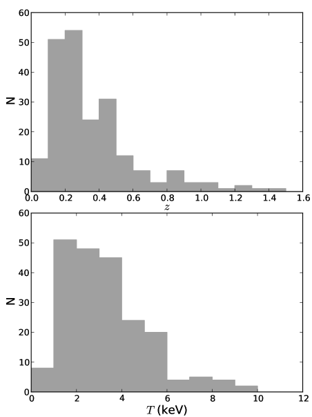
Figure 1: Redshift and temperature distributions for the sample of 211 XCS-DR1 clusters with spectroscopic redshifts used in this work (see Mehrtens et al., 2012, for a description of the catalogue).

In this work, we use only the subsample of 211 XCS-DR1 clusters with spectroscopic redshifts. While all of the data used in this paper is publicly available in the form of the XCS-DR1 catalogue, for completeness, the sample used here is listed in a supplementary table available with the online edition of this article. Fig. 1 shows the redshift and temperature distributions of the sample. The clusters span the redshift range 0.06–1.46 (median $z=0.28$), and temperature range 0.6–9.8 keV (median $T=2.9$ keV). Note that in the analysis presented in this paper, we do not attempt to correct for selection effects - given the redshift incompleteness of XCS (i.e., many candidate clusters within the survey area from which XCS-DR1 is drawn do not have optical follow-up or redshifts), accounting for selection biases is not straightforward, and is deferred to future work. We do however comment on the expected effect of Malmquist bias on our results for the $L_{\rm X}-T$ relation evolution in Section 5.1.

3 Analysis

The large size of the XCS-DR1 catalogue allows us to simultaneously fit for the redshift evolution of the $L_{\rm X}-T$ relation, in addition to its slope, normalisation and intrinsic scatter, using a model of the form

$$\log(E^{-1}(z)\,L_{\rm X})=A+B\log(T/5)+C\log(1+z),$$ (1)

where $L_{\rm X}$ is the bolometric X-ray luminosity measured within $R_{500}$ in erg s^-1 and $T$ is the X-ray temperature in keV. The advantage of this approach is that it avoids the need to bin the data by redshift. We set the pivot temperature to 5 keV for ease of comparison with other works (e.g. Pratt et al., 2009), although this is higher than the median temperature ($T=2.9$ keV) of the sample. This model assumes that the slope of the relation does not evolve with redshift. Note that we have scaled the luminosities by $E^{-1}(z)$ (the evolution of the Hubble parameter, i.e. $E(z)=[\Omega_{\rm m}(1+z)^{3}+\Omega_{\Lambda}]^{1/2}$), which is the evolution expected in the self-similar case, in which clusters are expected to become more luminous at fixed temperature as redshift increases. Hence $C=0$ corresponds to self-similar evolution, while $C<0$ indicates evolution which is slower than self-similar.

We estimate the parameters of this model using Markov Chain Monte Carlo (MCMC), using two different methods which both take into account the intrinsic scatter and the measurement errors. Our approach is similar to that of Weiner et al. (2006; see also Kelly 2007). Firstly, we define an orthogonal regression method, for which the probability density for a given cluster to be drawn from this model is

$$P_{\rm model}=\cfrac{1}{\sqrt{2\pi(\Delta r^{2}+S^{2})}}\exp\left[-\cfrac{(r-r_{\rm model})^{2}}{2(\Delta r^{2}+S^{2})}\right],$$ (2)

where $r-r_{\rm model}$ is the orthogonal distance of the cluster from the model relation in the $\log~{}L_{\rm X}$–$\log~{}T$ plane; $\Delta r$ is the error on the orthogonal distance, obtained from the projection in the direction orthogonal to the model line of the ellipse defined by the errors on $\log~{}L_{\rm X}$, $\log~{}T$ (appropriate sides of asymmetric error bars are chosen here according to the position of a given point relative to the model fit line); and $S$ is the (orthogonal) intrinsic scatter. The latter can be converted into the scatter in the $\log L_{\rm X}$ axis ($\sigma_{\log L_{\rm X}}$) using

$$\sigma_{\log L_{\rm X}}=S/\cos(\tan^{-1}B).$$ (3)

Table 1: Priors on $L_{\rm X}-T$ relation fit parameters (see Section 3).

Parameter	Uniform Prior	Notes
$A$	(41, 47)	-
$B$	(1, 5)	-
$C$	(-3, 3)	-
$S$	(0.01, 0.5)	Orthogonal method only
$\sigma_{\log L_{\rm X}}$	(0.01, 0.5)	Bisector method only
$\sigma_{\log T}$	(0.01, 0.5)	Bisector method only

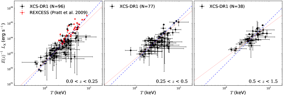
Figure 2: $L_{\rm X}-T$ relations for subsamples of XCS-DR1 in redshift bins. The dashed line shows the best fit to the data from the orthogonal method, while the dotted line shows the best fit according to the bisector method (see Section 3). The red triangles in the left hand panel show the REXCESS sample (Pratt et al., 2009) for comparison. Neither the slope nor scatter change significantly with redshift using the orthogonal method, while we see shallower slopes at high redshift using the bisector method (see Table 2).

Table 2: $L_{\rm X}-T$ relation fit parameters, derived from the bisector and orthogonal methods (see Section 3), for XCS-DR1 subsamples in redshift bins. The model fitted is $\log(E^{-1}(z)\,L_{\rm X})=A+B\log(T/5)$, and the units of $T$ and $L_{\rm X}$ are keV and erg s^-1 respectively. The uncertainties are the marginalised 68 per cent confidence regions on each parameter derived using MCMC.

		Bisector			Orthogonal
Redshift range	$N$	$A$	$B$	$\sigma_{\log L_{\rm X}}$	$A$	$B$	$\sigma_{\log L_{\rm X}}$
$0.0<z<0.25$	96	$44.43\pm 0.06$	$2.81\pm 0.14$	$0.40\pm 0.04$	$44.63\pm 0.10$	$3.18\pm 0.22$	$0.33\pm 0.04$
$0.25<z<0.5$	77	$44.36\pm 0.04$	$2.45\pm 0.14$	$0.33\pm 0.04$	$44.47\pm 0.07$	$2.82\pm 0.25$	$0.23\pm 0.04$
$0.5<z<1.5$	38	$44.23\pm 0.04$	$2.17\pm 0.19$	$0.24\pm 0.03$	$44.28\pm 0.07$	$2.89\pm 0.45$	$0.24\pm 0.05$

We also use a bisector method, in which the scatter and measurement errors in each axis are treated independently. In this case, $P_{\rm model}$ is the product of the Gaussian probabilities of the residuals of $L_{\rm X}$ and $T$ from the given bisector best-fitting line defined by the model parameters, i.e., we substitute

$$y_{\rm model}=\log(E^{-1}(z)\,L_{\rm X})-[A+B\log(T/5)+C\log(1+z)],$$ (4)

$$x_{\rm model}=\log(T/5)-[\log(E^{-1}(z)\,L_{\rm X})-A-C\log(1+z)]/B,$$ (5)

instead of $r_{\rm model}$ in Equation 2, and replace $r$, $\Delta r$ as appropriate. We replace $S$ with two parameters, $\sigma_{\log L_{\rm X}}$ and $\sigma_{\log T}$.

For both methods, the likelihood $\mathcal{L}$ of a given model is simply the product of $P_{\rm model}$ for each cluster in the sample, i.e., in the orthogonal case

$$\mathcal{L}(L_{\rm X},T|A,B,C,S)\propto P_{\rm prior}(A,B,C,S)\prod_{i}{P_{\rm model,\emph{i}}},$$ (6)

where we assume generous, uniform priors on each parameter, which are listed in Table 1. We obtain estimates of the model parameters from the posterior distributions using MCMC, implemented using the Metropolis et al. (1953) algorithm.

As shown in the next section, for $C=0$, the results given by the bisector and orthogonal methods are bracketed by those obtained when using the Kelly (2007) method, with $T$ alternately used as the dependent or independent variable. It is important to note that there is no single method which gives the ‘true’ underlying slope and normalisation for problems with errors in both variables and intrinsic scatter: each method gives a slope and normalisation which depends upon the assumptions in the method. Throughout this paper, we show the results from both methods, to give an idea of the possible systematic error arising from the choice of fitting method.

4 Results

4.1 Evolution of the slope and intrinsic scatter

The model for the evolution of the $L_{\rm X}-T$ relation defined in Equation 1 assumes that there is no evolution in the slope of the relation. We checked for this by fitting the $L_{\rm X}-T$ relation of subsamples divided into redshift bins ($0.0<z<0.25$, $0.25<z<0.5$, and $0.5<z<1.5$), setting $C=0$ in Equation 1. Fig. 2 and Table 2 show the results.

For the lowest redshift bin ($z<0.25$), we find a similar slope using both the orthogonal and bisector methods to that found in many previous studies. The values we derive are consistent with the value of $3.35\pm 0.32$ measured by REXCESS  (Pratt et al., 2009) at $z=0.1$, as well as numerous other works (e.g. Markevitch, 1998; Arnaud & Evrard, 1999; Wu et al., 1999), and most of the $z<0.3$ subsamples of XCS-DR1 clusters in the study by Stott et al. (2012), in which a different fitting technique was used.

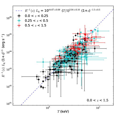
Figure 3: The $L_{\rm X}-T$ relation for the 211 XCS-DR1 clusters with spectroscopic redshifts. The dashed line is the best-fitting four parameter model (Equation 1), determined using the orthogonal fitting method. The luminosities have been scaled to take into account the evolution in the normalisation as a function of redshift inferred from the best-fitting model parameters, as well as the $E^{-1}(z)$ evolution expected in the self-similar case.

Figure 4: One and two dimensional marginalised distributions (contours mark 68 and 95 per cent confidence limits) for each combination of parameters in the four parameter evolving $L_{\rm X}-T$ relation model (Equation 1), as determined using the orthogonal fitting method. Note that the luminosities have been scaled by $E^{-1}(z)$, and so $C=0$ corresponds to the case of self-similar evolution.

We find different values for the normalisation, depending on the fitting technique employed. For the orthogonal method, we find $A=44.63\pm 0.10$, which is slightly lower, but within 2$\sigma$, of the REXCESS value ($44.85\pm 0.06$; Pratt et al., 2009). The normalisation obtained using the bisector method ($A=44.43\pm 0.06$) is about 5$\sigma$ lower than the REXCESS value. This seems to be driven by the degeneracy between the slope and normalisation, with the orthogonal method preferring steeper slopes. As can be seen in the left hand panel Fig. 2, the bisector method gives more weight to a population of low $L_{\rm X}$, but relatively high $T$ objects, resulting in a shallower slope and correspondingly lower normalisation.

Clearly, as shown in the left panel of Fig. 2, there is not much overlap between the XCS and REXCESS temperature ranges, so it is not surprising that there is some difference between the normalisations of the two samples. This may also be in part due to the use of the Cash (1979) rather than $\chi^{2}$ statistic in the XCS spectral fitting (LD11; see also Humphrey et al. 2009), or reflect differences in the sample selection, if for example the XCS sample contains a smaller fraction of cool core clusters, which prefer a higher normalisation (see, e.g., Table 2 of Pratt et al. (2009), where $A=45.11\pm 0.16$ for cool core clusters, while $A=44.70\pm 0.03$ for non-cool core clusters).

We find that both the bisector and orthogonal fit results are bracketed by those obtained using the Kelly (2007) method, depending on the choice of the dependent variable. With $T$ as the independent variable, we find $A=44.42\pm 0.09$ and $B=2.67\pm 0.19$, which is in good agreement with our bisector method, although with shallower slope. For $T$ as the dependent variable, we infer $A=44.70\pm 0.10$ and $B=3.38\pm 0.23$ using the Kelly (2007) method, which are in good agreement with our orthogonal method, although with slightly higher slope and normalisation.

The redshift evolution of the slope is different for the two fitting methods. For the orthogonal method, the slope does not change significantly with redshift, with the values found for each subsample differing by about $1\sigma$. This is consistent with the findings of previous studies, which have measured the slope at $z>0.4$ using smaller samples than that used in this work (e.g. Vikhlinin et al., 2002; Novicki et al., 2002; Ettori et al., 2004; Maughan et al., 2006, 2012; Takey et al., 2011). However, we do see flattening of the slope with increasing redshift in the fits using the bisector method. While this may be real, it is also an expected signature of Malmquist bias, which is discussed in Section 5.1.

The intrinsic scatter in the relation appears to decrease slightly with redshift (see Table 2), although the difference in the scatter between any two redshift bins (using either fitting method) is generally less than $2\sigma$. This suggests there might be a decreasing fraction of cool core clusters at high redshift, although of course better data are needed to determine if this is the case. We note that a decrease in the scatter at high redshift could alternatively be due to selection effects, as shown by Reichert et al. (2011) using simulated cluster samples. Our intrinsic scatter estimates for the lowest redshift bin are consistent with the REXCESS measurement at $z=0.1$ (Pratt et al., 2009).

We conclude, on the basis of these results, that it is reasonable to use a model with fixed slope and scatter to measure the evolution of the normalisation of the relation with redshift (which appears to evolve negatively in Fig. 2), when using the orthogonal fitting method. We also present the results obtained for the bisector method throughout, as this gives an indication of the possible systematic error due to the choice of fitting technique.

Table 3: $L_{\rm X}-T$ relation fit parameters, derived from the bisector and orthogonal methods (see Section 3), for the full XCS-DR1 cluster sample with spectroscopic redshifts. In all cases, the normalisation ($A$) is quoted at $T=5$ keV. The fits with $B$ fixed have the slope set to the value found for the appropriate $0.0<z<0.25$ sample and fitting method combination listed in Table 2. In all cases, the value of $C$ implies the evolution of the relation is below the self-similar expectation.

	Bisector				Orthogonal
Model	$A$	$B$	$C$	$\sigma_{\log L_{\rm X}}$	$A$	$B$	$C$	$\sigma_{\log L_{\rm X}}$
$B$ free:
$E^{-1}(z)\,L_{\rm X}\propto(1+z)^{C}$	$44.41\pm 0.05$	$2.64\pm 0.09$	$-0.5\pm 0.3$	$0.35\pm 0.02$	$44.67\pm 0.09$	$3.04\pm 0.16$	$-1.5\pm 0.5$	$0.27\pm 0.03$
$L_{\rm X}\propto(1+z)^{C}$	$44.38\pm 0.05$	$2.63\pm 0.09$	$\phantom{+}0.3\pm 0.3$	$0.34\pm 0.02$	$44.65\pm 0.09$	$3.03\pm 0.16$	$-0.7\pm 0.5$	$0.27\pm 0.03$
$L_{\rm X}\propto E(z)^{C}$	$44.41\pm 0.04$	$2.65\pm 0.09$	$\phantom{+}0.3\pm 0.3$	$0.34\pm 0.02$	$44.63\pm 0.07$	$3.02\pm 0.15$	$-0.9\pm 0.5$	$0.27\pm 0.03$
$B$ fixed:
$E^{-1}(z)\,L_{\rm X}\propto(1+z)^{C}$	$44.48\pm 0.04$	$2.81$	$-0.7\pm 0.3$	$0.36\pm 0.02$	$44.73\pm 0.07$	$3.18$	$-1.7\pm 0.4$	$0.28\pm 0.03$
$L_{\rm X}\propto(1+z)^{C}$	$44.46\pm 0.04$	$2.81$	$\phantom{+}0.1\pm 0.3$	$0.36\pm 0.02$	$44.70\pm 0.07$	$3.18$	$-0.9\pm 0.4$	$0.28\pm 0.03$
$L_{\rm X}\propto E(z)^{C}$	$44.47\pm 0.03$	$2.81$	$\phantom{+}0.0\pm 0.3$	$0.36\pm 0.02$	$44.68\pm 0.06$	$3.18$	$-1.2\pm 0.5$	$0.28\pm 0.03$

4.2 Evolution of the normalisation

We measure the evolution of the normalisation of the $L_{\rm X}-T$ relation by fitting the four parameter model described by Equation 1 to the complete sample of 211 clusters, with $C$ now allowed to vary. This is the first such measurement over this redshift range using clusters drawn from a single survey and analysed in a consistent way. Our large dataset allows us to fit for all parameters simultaneously, without fixing the normalisation to that measured in a different low redshift sample (e.g. Markevitch, 1998; Arnaud & Evrard, 1999), as has often been done in past studies of this type (e.g. Ettori et al., 2004; Maughan et al., 2006; Pacaud et al., 2007).

Since the bisector method shows a preference for shallower slopes at higher redshift, we focus first on the results obtained using the orthogonal fitting method. Fig. 3 presents the $L_{\rm X}-T$ relation for the whole sample, with $E^{-1}(z)\,L_{\rm X}$ scaled according to the redshift evolution inferred from the best-fitting model

$$\log(E^{-1}(z)\,L_{\rm X})=(44.67\pm 0.09)~{} +~{}(3.04\pm 0.16)~{}\log(T/5)$$

$$-~{}(1.5\pm 0.5)~{}\log(1+z),$$ (7)

with $S=0.085\pm 0.008$ (i.e., $\sigma_{\log L_{\rm X}}=0.27\pm 0.03$). Fig. 4 shows the one and two dimensional marginalised probability distributions for each parameter. We see, as expected given the model definition, that the slope, normalisation, and redshift evolution are all degenerate to some extent.

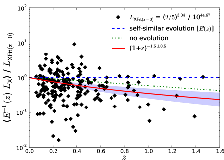
Figure 5: Evolution of the normalisation of the $L_{\rm X}-T$ relation relative to the self-similar case [$E(z)$], as inferred from the best-fitting four parameter model (Equation 7), using the orthogonal fitting method. The shaded area shows the marginalised 68 per cent confidence region on the evolution derived using MCMC. The dot-dashed line shows the track for no redshift evolution in the normalisation of the relation. The black diamonds show individual XCS clusters (error bars are omitted for clarity).

As for the fits to the subsamples in redshift bins (Section 4.1), the slope and scatter are consistent with low redshift samples. The $z=0$ normalisation inferred from the model ($A=44.67\pm 0.09$) is slightly lower than that found in REXCESS ($44.85\pm 0.06$; Pratt et al., 2009), but is consistent within less than $2\sigma$.

We find that the redshift evolution of the normalisation is negative ($C=-1.5\pm 0.5$), indicating that the evolution in luminosity at fixed temperature is significantly less than the self-similar prediction ($C=0$). However, the evolution we see is within $2\sigma$ of the no evolution case. This is shown graphically in Fig. 5. We checked the sensitivity of this result to reducing the redshift range, using a subsample of 183 clusters restricted to $z<0.6$. We find consistent results for all parameters, although the deviation of the normalisation from the self-similar prediction is not significant in this case ($C=-0.7\pm 0.9$), and is also consistent with null evolution to within less than $1\sigma$.

In Fig. 5, we see that the highest redshift cluster in our sample, J2215.9-1738 at $z=1.46$, has properties consistent with self-similar evolution. This is in contrast to our previous analysis of this cluster (Hilton et al., 2010), where we found it to be underluminous given its temperature. This is due to the assumption of the Markevitch (1998) $L_{\rm X}-T$ relation parameters in Hilton et al. (2010) when estimating the deviation of J2215.9-1738 from self-similarity. If we adopt the $L_{\rm X}$ and $T$ measurements from Hilton et al. (2010) for this system, and apply the best-fit $L_{\rm X}-T$ relation parameters derived in this work using the orthogonal MCMC method (i.e. $A=44.67\pm 0.09$, $B=3.04\pm 0.16$), then we find J2215.9-1738 is well within 1$\sigma$ of the self-similar prediction.

Repeating the analysis on the whole sample using the bisector method, we find that the redshift evolution ($C=-0.5\pm 0.3$) is closer to self-similar than we found using the orthogonal method. The milder evolution seen in this case seems to be driven by the much lower $z=0$ normalisation found using the bisector method ($A=44.41\pm 0.05$); this is significantly (approximately 5$\sigma$) lower than the REXCESS normalisation (see Section 4.1 above). Since the values of the slope and normalisation are degenerate, and we see from the results of Section 4.1 that the bisector method favours shallower slopes at high redshift, we repeated the fit with the value of the slope fixed to $B=2.81$, i.e., as found for the $0.0<z<0.25$ subsample (see Table 2). In this case, we find $C=-0.7\pm 0.3$. We conclude that, regardless of the fitting method, the XCS-DR1 data are consistent with negative evolution of the normalisation of the $L_{\rm X}-T$ relation with respect to the self-similar expectation.

Table 3 presents the fit parameters derived from the full sample using both the orthogonal and bisector methods. We show results for fits with $B$ as a free parameter, and with $B$ fixed to the slope found using the $0.0<z<0.25$ subsample. For ease of comparison with other works, we also list results using other common parametrisations for the evolution of the $L_{\rm X}-T$ relation in the literature.

As noted in Section 1, while there have been several previous estimates for the evolution of the normalisation of the $L_{\rm X}-T$ relation, there is no consensus. Our result is in good agreement with the negative evolution of the relation found by Reichert et al. (2011) from a heterogeneous compilation of 14 datasets, including the $z>0.8$ XMM Distant Cluster Project (XDCP; Fassbender et al., 2011) sample, as well as the findings of Ettori et al. (2004) and Clerc et al. (2012). Pacaud et al. (2007) find evolution consistent with self-similar from a sample of 24 clusters discovered in the XMM-LSS survey, after correcting for selection effects, which is consistent with our result given the large error bar on their measurement. Maughan et al. (2012) recently examined the $L_{\rm X}-T$ relation using a heterogeneous sample of 114 clusters drawn from the Chandra archive, and find evolution consistent with self-similar at $z>0.6$, after excising emission from cluster cores. Several other studies, based on much smaller samples, have found positive evolution, significantly different to that which we see here (e.g. Vikhlinin et al., 2002; Lumb et al., 2004; Kotov & Vikhlinin, 2005), while our result is in mild tension with the results of Novicki et al. (2002) and Maughan et al. (2006). However, as noted by many authors, the evolution inferred is dependent upon the choice of local $L_{\rm X}-T$ relation used to set the $z=0$ slope and normalisation used in these works.

The main difference between the sample used here in comparison to previous works (with the exception of Reichert et al. 2011) is the larger number of high redshift ($z>0.6$) clusters, and it is clear from Fig. 5 that a long redshift baseline is needed to constrain the evolution of the relation. It will be important to take into account both selection effects and the cluster mass function in order to reach a definitive conclusion. In the near future, it will be interesting to compare to measurements of the evolution of this relation using Sunyaev-Zel’dovich effect selected cluster samples (e.g. Andersson et al., 2011), once the number of such objects with X-ray follow-up becomes large enough.

5 Discussion

5.1 Influence of selection effects and the cluster mass function

An important limitation of the analysis we have presented in this paper is that the selection function of the survey is not taken into account. While modelling of the selection function for XCS has been performed (see Sahlén et al., 2009, LD11), the optical follow-up required for confirmation and redshift measurements is not complete (Mehrtens et al., 2012), meaning that it is not currently possible to perform a more sophisticated analysis that jointly fits for both cosmological and scaling relation parameters, while taking the selection function into account (e.g. Mantz et al., 2010). The most likely selection effect that could impact our results is Malmquist bias. For flux-limited samples, this is well known to give shallower slopes, and larger normalisations, in scaling relations, if left uncorrected (see e.g. Section 2.5 of the review by Allen, Evrard & Mantz, 2011), as a consequence of objects below a luminosity threshold being excluded from the sample. We note that the decreasing slope with redshift seen in the fits to the XCS-DR1 sample using the bisector method (Section 4.1) is likely to be a manifestation of this bias.

Pacaud et al. (2007) investigated the effect of accounting for the selection function in their measurement of the evolution of the $L_{\rm X}-T$ relation using the XMM-LSS sample. Their sample covers a similar redshift range to XCS-DR1 ($0.05<z<1.05$), but is extracted from a survey area of only 5 deg², and so contains only 24 clusters, with 7 at $z>0.6$. With the selection function excluded from their analysis, Pacaud et al. (2007) found positive evolution of the $L_{\rm X}-T$ relation with respect to self-similar ($C=1.5\pm 0.4$, for a model of the form $L_{\rm X}\propto(1+z)^{C}$, i.e. without scaling the $L_{\rm X}$ values by $E^{-1}(z)$), which is significantly different to our results (see Table 3). This may be due to the different depths of the two surveys, since XCS has searched a large number of XMM observations with longer exposure times than XMM-LSS (see Fig. 5 of LD11). However, after accounting for selection effects, Pacaud et al. (2007) find much milder evolution, which is almost exactly self-similar (although with large uncertainty). This demonstrates that inclusion of the selection function in the analysis acts to drive the inferred evolution in a negative direction. Therefore it does not seem possible for uncorrected Malmquist bias to explain the negative evolution with respect to self-similar that we see.

We have also not attempted to take into account in the analysis the effect of the (theoretically expected) underlying cluster distribution as a function of mass and redshift. To do this, in principle, we would have to assume a prior probability for the cluster temperatures and luminosities, which would be a decreasing function of such quantities. Given that the uncertainty in our temperature estimates tends to increase faster with redshift than the uncertainty in our luminosity estimates, it may be that the end result of taking into account such an effect would be a less pronounced negative evolution of the normalisation of the $L_{\rm X}-T$ relation. However, the size of this effect also depends on the full XCS selection function, including follow-up incompleteness, the effect of which is likely to mitigate this bias to some extent. We have therefore decided to defer a more detailed analysis which will quantify the size of this effect to future work, once we have a better understanding of the XCS follow-up incompleteness.

5.2 Influence of cool cores, AGN, and group fraction

Another limitation, due to the serendipitous data used in this analysis, is that the low number of counts detected for each cluster, coupled to the low resolution off-axis and the high redshift of our sources (Section 2), makes it unfeasible to excise the core emission from clusters, or divide the sample into cool-core and non-cool core populations (e.g. Pratt et al., 2009; Maughan et al., 2012).

This could affect our results in one of two ways. On one hand, cool core clusters are generally easier to detect than non-cool core clusters, due to their increased central densities. In this case, it could be the case that the XCS sample includes a higher fraction of cool cores than the true underlying cluster population, particularly at high redshift. This seems not to be the case, because we see negative evolution of the $L_{\rm X}-T$ relation normalisation, and cool core clusters are known to have a higher $L_{\rm X}-T$ relation normalisation than the non-cool core population (Pratt et al., 2009).

On the other hand, it may be that cool core clusters at high redshift are under-represented in our sample, due to being classified as point sources, rather than extended objects, by the detection pipeline (described in LD11). This could then contribute to the negative evolution of the normalisation that we see. However, simulations in which model cool core clusters are inserted into real XMM observations show that this is not a significant issue for objects detected with more than 500 counts (LD11). Since the sample used in this work contains many objects detected with $<500$ counts, we repeated our analysis using the subsample of 108 clusters with $>500$ counts. We find results consistent with those found from the whole sample (Table 3), with $C=-1.6\pm 0.6$ using the orthogonal method, and $C=-1.1\pm 0.4$ for the bisector method (for a model in the form of Equation 1). We conclude that it is unlikely that a missing fraction of cool core clusters in our sample could explain our results - although it is possible that a real evolution in the cool core fraction could cause the evolution that we see, if cool cores are less common at high redshift.

Similarly, although we are able to detect and excise point source emission from clusters at low redshift, this naturally becomes increasingly difficult at high redshift, where it may be the case that contamination by AGNs is common, as the space density of X-ray AGNs increases significantly with redshift (e.g. Silverman et al., 2005). Unaccounted for AGN contamination could have the effect of hardening the X-ray spectra, leading to overestimated cluster temperatures, which could explain the negative $L_{\rm X}-T$ relation normalisation evolution that we see, if it affects the majority of the sample. These issues can only be addressed through higher resolution X-ray imaging of the high redshift XCS cluster sample (e.g. Hilton et al., 2010); however, it will be possible to investigate these concerns for a small fraction of the sample with overlapping observations in the Chandra archive. We note that a stacking analysis in the directions of $z>0.9$ clusters by Fassbender, Suhada & Nastasi (2012) has examined this issue using XMM-Newton data, and finds on average one AGN within 1 Mpc cluster-centric distance per cluster. While this level of contamination is thought unlikely to have a significant effect on cluster flux measurements and sample selection, the importance of this potential bias on temperature estimates for objects in this redshift range has yet to be quantified.

It may be the case that there is a break in the cluster scaling laws below a certain mass or temperature threshold, due perhaps to a change in the physics affecting the ICM between the group and cluster regimes (e.g. Helsdon & Ponman, 2000; Sun et al., 2009; Stott et al., 2012). Similarly, Maughan et al. (2012) see evidence for a break in the $L_{\rm X}-T$ relation for high temperature ($T>3.5$ keV), relaxed systems, which seem to follow a relation consistent with the self-similar slope ($B=2$), whereas lower temperature, unrelaxed systems form a steeper relation. However, this effect is only seen after the excision of core emission, which is not something that can be investigated with our data. Given that our sample contains a number of low temperature ($T<2$ keV) systems, and that the fraction of low temperature systems decreases as redshift increases (Figs. 2 and 3), we repeat our analysis on the subsample of 149 $T>2$ keV clusters. Using both fitting methods, we find that such a cut in temperature leads to steeper slopes ($B=3.8\pm 0.3$ and $B=3.0\pm 0.2$ for the orthogonal and bisector methods respectively), but does not change the inferred negative evolution of the $L_{\rm X}-T$ relation normalisation: we find $C=-1.8\pm 0.6$ using the orthogonal method, and $C=-0.8\pm 0.4$ using the bisector method, both of which are in excellent agreement with the results obtained using the full sample of 211 clusters.

5.3 Comparison with numerical simulations

Under the assumption that neither selection effects (Section 5.1), nor a missing cool core population or significant AGN contamination (Section 5.2), can explain the negative evolution of the $L_{\rm X}-T$ relation normalisation that we see, we now consider the implications of our results for cosmological simulations of galaxy clusters. We do this by comparing to several simulations, which predict similar $L_{\rm X}-T$ relations at $z=0$, but which behave quite differently at high redshift, as a result of the choices made in modelling the heating and cooling of the intracluster medium.

5.3.1 Simulations

Below we briefly describe the features of the models to which we compare.

Table 4: $L_{\rm X}-T$ relation fit parameters, derived from the bisector and orthogonal methods (see Section 3), for simulated cluster samples with redshift distribution matched to the XCS-DR1 spectroscopic sample used in this work. The simulations are: CLEF (Kay et al., 2007); the Millennium Gas simulations, for which MG1-GO = gravity only, MG1-FO = feedback only, and MG1-PC = precooling (see Short et al., 2010); and a new version of the Millennium Gas simulation with an updated feedback prescription (MG2-FO; Short, Thomas & Young 2012). The fitted model is of the form $\log(E^{-1}(z)\,L_{\rm X})=A+B\log(T/5)+C\log(1+z)$. The fits with $B$ fixed have the slope set to the value found from an ordinary least squares fit to the simulated sample at $z=0$. Note that although the two fitting methods give significantly different values for the slope and $z=0$ normalisation in some cases, there is good agreement between the methods on the value of the redshift evolution parameter, $C$.

	Bisector				Orthogonal
Simulation	$A$	$B$	$C$	$\sigma_{\log L_{\rm X}}$	$A$	$B$	$C$	$\sigma_{\log L_{\rm X}}$
$B$ free:
CLEF	$45.31\pm 0.04$	$3.49\pm 0.10$	$-1.42\pm 0.15$	$0.211\pm 0.011$	$45.41\pm 0.06$	$3.99\pm 0.19$	$-1.25\pm 0.24$	$0.265\pm 0.019$
MG1-GO	$45.93\pm 0.03$	$2.67\pm 0.10$	$\phantom{+}0.16\pm 0.10$	$0.144\pm 0.008$	$46.12\pm 0.06$	$3.27\pm 0.18$	$\phantom{+}0.09\pm 0.13$	$0.156\pm 0.012$
MG1-FO	$44.80\pm 0.02$	$3.12\pm 0.05$	$\phantom{+}0.66\pm 0.08$	$0.104\pm 0.006$	$44.78\pm 0.02$	$3.23\pm 0.07$	$\phantom{+}0.74\pm 0.12$	$0.113\pm 0.007$
MG1-PC	$44.95\pm 0.02$	$3.92\pm 0.06$	$-2.20\pm 0.06$	$0.088\pm 0.005$	$44.96\pm 0.03$	$3.94\pm 0.08$	$-2.19\pm 0.08$	$0.088\pm 0.006$
MG2-FO	$44.44\pm 0.02$	$2.68\pm 0.04$	$\phantom{+}1.82\pm 0.07$	$0.094\pm 0.006$	$44.48\pm 0.02$	$2.79\pm 0.07$	$\phantom{+}1.79\pm 0.10$	$0.099\pm 0.006$
$B$ fixed:
CLEF	$45.23\pm 0.03$	$3.08$	$-1.54\pm 0.14$	$0.212\pm 0.011$	$45.26\pm 0.04$	$3.08$	$-1.68\pm 0.19$	$0.208\pm 0.011$
MG1-GO	$45.72\pm 0.02$	$2.00$	$\phantom{+}0.21\pm 0.09$	$0.133\pm 0.007$	$45.76\pm 0.02$	$2.00$	$\phantom{+}0.04\pm 0.13$	$0.131\pm 0.007$
MG1-FO	$44.79\pm 0.01$	$3.30$	$\phantom{+}0.70\pm 0.07$	$0.114\pm 0.006$	$44.77\pm 0.02$	$3.30$	$\phantom{+}0.82\pm 0.11$	$0.113\pm 0.007$
MG1-PC	$44.76\pm 0.01$	$3.30$	$-2.10\pm 0.07$	$0.096\pm 0.005$	$44.77\pm 0.02$	$3.30$	$-2.13\pm 0.10$	$0.097\pm 0.006$
MG2-FO	$44.48\pm 0.01$	$2.79$	$\phantom{+}1.74\pm 0.07$	$0.091\pm 0.005$	$44.47\pm 0.02$	$2.79$	$\phantom{+}1.79\pm 0.09$	$0.095\pm 0.006$

CLEF (Kay et al., 2007) is a hydrodynamical simulation of a 200$h^{-1}$ Mpc comoving box which includes radiative cooling and feedback. The latter is implemented using the ‘strong feedback’ model of Kay (2004). The amount of energy injection in this model effectively tracks the star formation rate - a fraction of the particles which pass both a density and temperature threshold are assigned an entropy of 1000 keV cm², which is then distributed through the ICM through viscous interactions and shocks. This model produces cool core clusters at low redshift, which disappear as redshift increases, leading to a reduction in the scatter about the relation at high redshift.

The Millennium Gas project (Short et al., 2010) is a suite of hydrodynamical simulations which use the same volume (500$h^{-1}$ Mpc³) and initial perturbations as the Millennium Simulation (Springel et al., 2005). This set of simulations includes a gravity only ‘control’ model (MG1-GO); a simulation with energy injection at high redshift and radiative cooling (we refer to this as the ‘precooling’ model, or MG1-PC); and a simulation which incorporates feedback from AGN and supernovae, implemented using a semi-analytic model (MG1-FO).

The MG1-PC simulation implements preheating of the cluster gas at high redshift in a similar fashion to previous work (e.g. Bialek et al., 2001; Borgani et al., 2002). In this case, the entropy of each gas particle is raised to 200 keV cm² at $z=4$. While this model is not physically plausible (only two per cent of the baryons form stars by $z=0$, and the model is incapable of forming cool core clusters; Short et al. 2010), it does reproduce the $L_{\rm X}-T$ relation at $z=0$ (Hartley et al., 2008).

The MG1-FO model includes supernova and AGN feedback using the scheme of Short & Thomas (2009), where the semi-analytic galaxy formation model employed by De Lucia & Blaizot (2007) is used to infer both the star formation rate (a sink of hot gas) and the heating rate due to supernovae and AGN. The AGN feedback is implemented using the scheme suggested by Bower et al. (2008) and is capped at two per cent of the Eddington rate (see Short et al. 2010 for full details). The model successfully reproduces both the local $L_{\rm X}-T$ relation (Short et al., 2010), and the Sunyaev-Zel’dovich $Y-M$ relation (Kay et al., 2012).

We also compare to an updated version of the Millennium Gas model with AGN feedback (MG2-FO). This run was performed using a 250$h^{-1}$ Mpc box with higher resolution and updated cosmological parameters (consistent with the WMAP 7-year results; Komatsu et al. 2011). The semi-analytic galaxy formation model is also newer (Guo et al., 2011), and the feedback is now implemented in a stochastic fashion (only a fraction of the intracluster gas particles are heated directly, whereas in the previous model the energy was shared throughout the cluster). The model improves agreement with non cool-core clusters but, like the previous Millennium Gas models, fails to produce the cool-core population due to the absence of radiative cooling. Full details of this implementation are discussed in Short, Thomas & Young (2012).

5.3.2 Results

All of the simulations described above provide measurements that are comparable to the real XCS-DR1 data. In all cases, we use total (i.e. core included) bolometric luminosity measurements within $R_{500}$, which is defined with respect to the critical density, as for the XCS-DR1 measurements. We note that each of these simulations assumes a slightly different cosmology to the one assumed in this work. We have neglected to correct the luminosities to account for this, as it is a small effect, and does not significantly affect the evolution of the normalisation of the relation, which differs substantially between the models, due to the different physical assumptions in each.

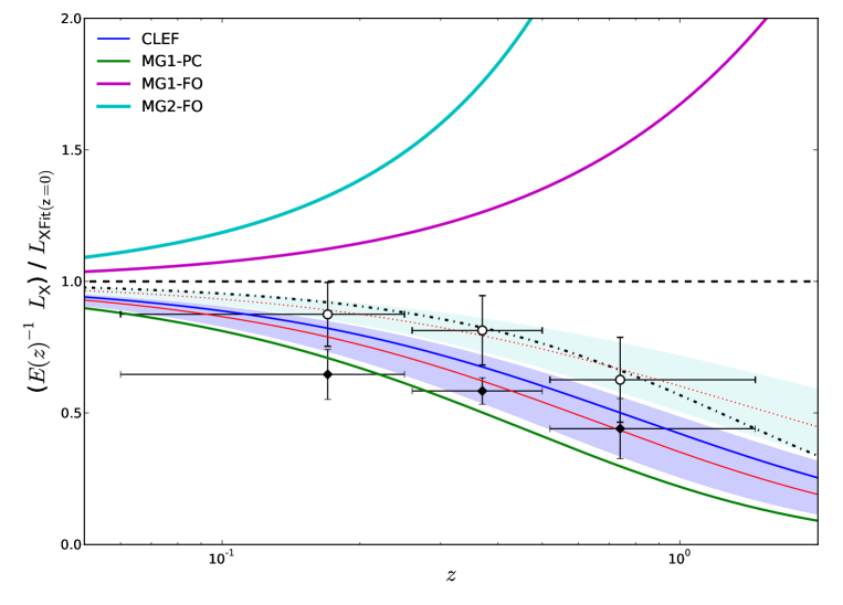
Figure 6: Evolution of the normalisation of the $L_{\rm X}-T$ relation as measured from XCS-DR1, compared with numerical simulations (indicated in the legend; see Section 5.3 and Table 4 for details). The solid thin red line is the best-fit obtained from XCS-DR1 using the orthogonal method, while the black diamonds show the corresponding median values for the clusters in each redshift bin (horizontal error bars indicate the redshift range of each bin, while vertical error bars indicate the 1$\sigma$ uncertainty in the median, estimated using bootstrap resampling). The dotted thin red line similarly represents the best-fit for XCS-DR1 obtained using the bisector method, with the slope fixed at the $z=0$ value (2.81, see Table 3), and the open circles indicate the median values for clusters in redshift bins for this set of best-fit $L_{\rm X}-T$ relation parameters. This latter fit is consistent with no evolution (dot-dashed line). The shaded regions mark the marginalised 68 per cent confidence regions. While the amount of evolution inferred from the XCS sample depends on the fitting technique used, there is no such dependence for the simulated data (see Table 4), and so we only show the results of the fits to the simulations using the orthogonal method. The XCS data favour negative evolution with respect to self-similar ($E(z)$; horizontal dotted line), and are clearly better described by the CLEF or MG1-PC models, rather than the models which implement AGN and supernovae feedback using a semi-analytic prescription (MG1-FO and MG2-FO).

All of the simulations provide spectroscopic-like temperature estimates ($T_{\rm sl}$; Mazzotta et al., 2004). We restrict our analysis in all cases to clusters with $T_{\rm sl}>2$ keV, as this is the regime in which the bremsstrahlung mechanism dominates, and is where the spectroscopic-like temperatures are most robust. Objects identified as satellites to more massive haloes are not included in the samples we draw from the simulations.

For consistency with the analysis of the XCS data, we draw random samples from each simulation with redshift distributions matched to that of XCS-DR1 (Fig. 1), and we fit each sample using both the orthogonal and bisector methods, as before. Table 4 lists the results. As is the case for the real data, for some simulations (e.g. CLEF), the bisector and orthogonal methods give different slopes and normalisations, with the orthogonal slope being steeper. However, we see that in all cases, both methods give consistent values for the redshift evolution parameter, $C$. The better agreement in $C$ between the two fitting methods, when used on the simulations as compared to the real data, is likely to be due to the absence of selection effects in the former.

In some cases, we find steeper slopes than were measured in the original works describing the simulations, most notably in the MG1-GO case, where $B=2$ is expected. This is due to our fitting methods (both Kay et al. 2007 and Short et al. 2010 use ordinary least squares regression). We checked that this does not bias our estimates of $C$, by repeating the fitting with the slope ($B$) fixed to the values found in Kay et al. (2007) and Short et al. (2010) from the complete simulated samples. These results are also listed in Table 4. In all cases, when $B$ is fixed, the values of $C$ change by at most 2$\sigma$ in comparison to the fits with $B$ as a free parameter. In no case do we find qualitatively different behaviour for a given model as a result of changing the fitting technique or fixing the slope: e.g., we find negative evolution of the $L_{\rm X}-T$ relation in CLEF for all the variations.

Fig. 6 shows a comparison of the redshift evolution in the simulations with the results from the XCS-DR1 sample, where we show the results for both the orthogonal fitting method, and the bisector method with slope fixed to the $z=0$ value (see Section 4.1 and Table 3). This gives an indication of the systematic uncertainty in the XCS-DR1 measurement due to the choice of the fitting method. We see that in either case the XCS-DR1 data are closer to the CLEF and MG1-PC simulations, in which the $L_{\rm X}-T$ normalisation evolves negatively with respect to self-similar, and are more than $5\sigma$ away from the evolution predicted in the MG1-FO and MG2-FO simulations (irrespective of the fitting method used on the XCS-DR1 data).

The key difference between the feedback models in the simulation is the epoch at which most of the energy injection occurs. In the MG1-PC model, all of the energy input occurs at $z=4$, which is not likely to be physically reasonable, but serves as a useful extreme test. In the CLEF simulation, the energy injection occurs over a broad range of redshifts, but is skewed to early times, as it directly tracks the star formation rate (around two thirds of the stars have already formed, and energy injected, by $z=1$). Finally, in the MG1-FO and MG2-FO simulations, the dominant AGN feedback occurs later, when the black holes have grown to sufficient mass to act as powerful energy sources. Therefore, the lack of agreement with the observations suggests that feedback at high redshift is too inefficient in the current models. We note also that radiative cooling is not currently implemented in these simulations, and therefore the cold gas mass growth rate in the semi-analytic model is not fully self consistent with the hydrodynamical simulation.

6 Conclusions

We have investigated the evolution of the $L_{\rm X}-T$ relation since $z\sim 1.5$ using a sample of 211 spectroscopically confirmed X-ray clusters drawn from the first XCS data release (Mehrtens et al., 2012). This is the first such measurement over this wide redshift range using a single, homogeneous sample. We find:

1. Using both an orthogonal and bisector fitting method, the slope of the $L_{\rm X}-T$ relation for the $z<0.25$ subsample of XCS-DR1 clusters is consistent with that found for the REXCESS sample (Pratt et al., 2009). The normalisation is slightly lower, but consistent within $2\sigma$, using the orthogonal method, although we find a 5$\sigma$ lower normalisation using the bisector method. This may be in part due to differences in the spectral fitting, or could be due to differences in the sample selection.

2. From dividing the sample into redshift bins, using the orthogonal fitting method, we see no evidence for evolution in either the slope or intrinsic scatter as redshift increases - both are consistent with previous measurements at $z=0.1$. We see a flattening of the slope at high redshift when using the bisector fitting method, which could be a signature of the effect of Malmquist bias.

3. Regardless of the fitting method, our data shows that the normalisation of the relation evolves negatively with respect to self-similar. For the orthogonal method, we find the evolution is $E^{-1}(z)\,L_{\rm X}=10^{44.67\pm 0.09}(T/5)^{3.04\pm 0.16}(1+z)^{-1.5\pm 0.5}$, which is within $2\sigma$ of the zero evolution case. Using the bisector method, with the slope fixed to the value found for the $z<0.25$ subsample, we find $E^{-1}(z)\,L_{\rm X}\propto T^{2.81}(1+z)^{-0.7\pm 0.3}$. Malmquist bias would have the effect of driving the normalisation in the positive direction, and so cannot explain this result. It is possible that a deficit of cool cores in the XCS-DR1 sample, or significant AGN contamination at high redshift, may contribute to the negative evolution that we see. The former seems unlikely, given that a higher signal-to-noise subsample gives consistent results to those obtained using the full sample, while the latter can only be tested using higher resolution X-ray data.

4. From comparison with numerical simulations, we find the XCS-DR1 data favour feedback models in which the majority of the energy injection occurs at high redshift. AGN feedback models based on current semi-analytic galaxy formation model prescriptions, as used in the Millennium Gas project, predict positive evolution with respect to self-similar, and differ from the XCS-DR1 measurements at the $>5\sigma$ level. This suggests that feedback at high redshift in these models is too inefficient.

A more sophisticated analysis to jointly constrain both cosmological and scaling relation parameters, taking into account both a model of the survey selection function and the cluster mass function, will be possible with improved redshift completeness. We are also pursuing velocity dispersion measurements of the high redshift XCS cluster sample, and will explore the evolution of the scaling of X-ray observables with dynamical mass in future work.

References

- Allen et al. (2011) Allen S. W., Evrard A. E., Mantz A. B., 2011, ARA&A, 49, 409
- Andersson et al. (2011) Andersson K., et al., 2011, ApJ, 738, 48
- Arnaud (1996) Arnaud K. A., 1996, in G. H. Jacoby & J. Barnes ed., Astronomical Data Analysis Software and Systems V Vol. 101 of Astronomical Society of the Pacific Conference Series, XSPEC: The First Ten Years. p. 17
- Arnaud & Evrard (1999) Arnaud M., Evrard A. E., 1999, MNRAS, 305, 631
- Bialek et al. (2001) Bialek J. J., Evrard A. E., Mohr J. J., 2001, ApJ, 555, 597
- Bîrzan et al. (2004) Bîrzan L., Rafferty D. A., McNamara B. R., Wise M. W., Nulsen P. E. J., 2004, ApJ, 607, 800
- Blanton et al. (2011) Blanton E. L., Randall S. W., Clarke T. E., Sarazin C. L., McNamara B. R., Douglass E. M., McDonald M., 2011, ApJ, 737, 99
- Borgani et al. (2002) Borgani S., Governato F., Wadsley J., Menci N., Tozzi P., Quinn T., Stadel J., Lake G., 2002, MNRAS, 336, 409
- Bower et al. (2008) Bower R. G., McCarthy I. G., Benson A. J., 2008, MNRAS, 390, 1399
- Cash (1979) Cash W., 1979, ApJ, 228, 939
- Cavaliere & Fusco-Femiano (1976) Cavaliere A., Fusco-Femiano R., 1976, A&A, 49, 137
- Clerc et al. (2012) Clerc N., Sadibekova T., Pierre M., Pacaud F., Le Fèvre J.-P., Adami C., Altieri B., Valtchanov I., 2012, MNRAS, in press (doi:10.1111/j.1365-2966.2010.18033.x)
- De Lucia & Blaizot (2007) De Lucia G., Blaizot J., 2007, MNRAS, 375, 2
- Edge & Stewart (1991) Edge A. C., Stewart G. C., 1991, MNRAS, 252, 414
- Ettori et al. (2004) Ettori S., Tozzi P., Borgani S., Rosati P., 2004, A&A, 417, 13
- Fassbender et al. (2011) Fassbender R., Böhringer H., Nastasi A., Šuhada R., Mühlegger M., de Hoon A., Kohnert J., Lamer G., Mohr J. J., Pierini D., Pratt G. W., Quintana H., Rosati P., Santos J. S., Schwope A. D., 2011, New Journal of Physics, 13, 125014
- Fassbender et al. (2012) Fassbender R., Suhada R., Nastasi A., 2012, Advances in Astronomy, in press (arXiv:1203.5337)
- Guo et al. (2011) Guo Q., White S., Boylan-Kolchin M., De Lucia G., Kauffmann G., Lemson G., Li C., Springel V., Weinmann S., 2011, MNRAS, 413, 101
- Harrison et al. (2012) Harrison C. D., Miller C. J., Richards J. W., Lloyd-Davies E. J., Hoyle B., Romer A. K., Mehrtens N., Hilton M., Stott J. P., Capozzi D., Collins C. A., Deadman P.-J., Liddle A. R., Sahlén M., Stanford S. A., Viana P. T. P., 2012, ApJ, 752, 12
- Hartley et al. (2008) Hartley W. G., Gazzola L., Pearce F. R., Kay S. T., Thomas P. A., 2008, MNRAS, 386, 2015
- Helsdon & Ponman (2000) Helsdon S. F., Ponman T. J., 2000, MNRAS, 315, 356
- Hilton et al. (2007) Hilton M., et al., 2007, ApJ, 670, 1000
- Hilton et al. (2009) Hilton M., et al., 2009, ApJ, 697, 436
- Hilton et al. (2010) Hilton M., et al., 2010, ApJ, 718, 133
- Humphrey et al. (2009) Humphrey P. J., Liu W., Buote D. A., 2009, ApJ, 693, 822
- Kaiser (1986) Kaiser N., 1986, MNRAS, 222, 323
- Kay (2004) Kay S. T., 2004, MNRAS, 347, L13
- Kay et al. (2007) Kay S. T., da Silva A. C., Aghanim N., Blanchard A., Liddle A. R., Puget J.-L., Sadat R., Thomas P. A., 2007, MNRAS, 377, 317
- Kay et al. (2012) Kay S. T., Peel M. W., Short C. J., Thomas P. A., Young O. E., Battye R. A., Liddle A. R., Pearce F. R., 2012, MNRAS, 422, 1999
- Kelly (2007) Kelly B. C., 2007, ApJ, 665, 1489
- Komatsu et al. (2011) Komatsu E., et al., 2011, ApJS, 192, 18
- Kotov & Vikhlinin (2005) Kotov O., Vikhlinin A., 2005, ApJ, 633, 781
- Lloyd-Davies et al. (2011) Lloyd-Davies E. J., et al., 2011, MNRAS, 418, 14
- Lumb et al. (2004) Lumb D. H., et al., 2004, A&A, 420, 853
- Mantz et al. (2010) Mantz A., Allen S. W., Ebeling H., Rapetti D., Drlica-Wagner A., 2010, MNRAS, 406, 1773
- Mantz et al. (2010) Mantz A., Allen S. W., Rapetti D., Ebeling H., 2010, MNRAS, 406, 1759
- Markevitch (1998) Markevitch M., 1998, ApJ, 504, 27
- Maughan et al. (2012) Maughan B. J., Giles P. A., Randall S. W., Jones C., Forman W. R., 2012, MNRAS, 421, 1583
- Maughan et al. (2006) Maughan B. J., Jones L. R., Ebeling H., Scharf C., 2006, MNRAS, 365, 509
- Mazzotta et al. (2004) Mazzotta P., Rasia E., Moscardini L., Tormen G., 2004, MNRAS, 354, 10
- McCarthy et al. (2011) McCarthy I. G., Schaye J., Bower R. G., Ponman T. J., Booth C. M., Dalla Vecchia C., Springel V., 2011, MNRAS, 412, 1965
- McNamara et al. (2005) McNamara B. R., Nulsen P. E. J., Wise M. W., Rafferty D. A., Carilli C., Sarazin C. L., Blanton E. L., 2005, Nature, 433, 45
- Mehrtens et al. (2012) Mehrtens N., et al., 2012, MNRAS, 423, 1024
- Metropolis et al. (1953) Metropolis N., Rosenbluth A. W., Rosenbluth M. N., Teller A. H., Teller E., 1953, J. Chem. Phys., 21, 1087
- Muanwong et al. (2006) Muanwong O., Kay S. T., Thomas P. A., 2006, ApJ, 649, 640
- Novicki et al. (2002) Novicki M. C., Sornig M., Henry J. P., 2002, AJ, 124, 2413
- Pacaud et al. (2007) Pacaud F., et al., 2007, MNRAS, 382, 1289
- Planck Collaboration (2011) Planck Collaboration 2011, A&A, 536, A8
- Pratt et al. (2009) Pratt G. W., Croston J. H., Arnaud M., Böhringer H., 2009, A&A, 498, 361
- Reichert et al. (2011) Reichert A., Böhringer H., Fassbender R., Mühlegger M., 2011, A&A, 535, A4
- Romer et al. (2001) Romer A. K., Viana P. T. P., Liddle A. R., Mann R. G., 2001, ApJ, 547, 594
- Sahlén et al. (2009) Sahlén M., et al., 2009, MNRAS, 397, 577
- Short & Thomas (2009) Short C. J., Thomas P. A., 2009, ApJ, 704, 915
- Short et al. (2012) Short C. J., Thomas P. A., Young O. E., 2012, MNRAS submitted (arXiv:1201.1104)
- Short et al. (2010) Short C. J., Thomas P. A., Young O. E., Pearce F. R., Jenkins A., Muanwong O., 2010, MNRAS, 408, 2213
- Silverman et al. (2005) Silverman J. D., Green P. J., Barkhouse W. A., Cameron R. A., Foltz C., Jannuzi B. T., Kim D., Kim M., Mossman A., Tananbaum H., Wilkes B. J., Smith M. G., Smith R. C., Smith P. S., 2005, ApJ, 624, 630
- Springel et al. (2005) Springel V., White S. D. M., Jenkins A., Frenk C. S., Yoshida N., Gao L., Navarro J., Thacker R., Croton D., Helly J., Peacock J. A., Cole S., Thomas P., Couchman H., Evrard A., Colberg J., Pearce F., 2005, Nature, 435, 629
- Stanford et al. (2006) Stanford S. A., et al., 2006, ApJL, 646, L13
- Stott et al. (2012) Stott J. P., et al., 2012, MNRAS, 422, 2213
- Sun et al. (2009) Sun M., Voit G. M., Donahue M., Jones C., Forman W., Vikhlinin A., 2009, ApJ, 693, 1142
- Takey et al. (2011) Takey A., Schwope A., Lamer G., 2011, A&A, 534, A120
- Viana et al. (2012) Viana P. T. P., et al., 2012, MNRAS, 422, 1007
- Vikhlinin et al. (2006) Vikhlinin A., Kravtsov A., Forman W., Jones C., Markevitch M., Murray S. S., Van Speybroeck L., 2006, ApJ, 640, 691
- Vikhlinin et al. (2009) Vikhlinin A., Kravtsov A. V., Burenin R. A., Ebeling H., Forman W. R., Hornstrup A., Jones C., Murray S. S., Nagai D., Quintana H., Voevodkin A., 2009, ApJ, 692, 1060
- Vikhlinin et al. (2002) Vikhlinin A., van Speybroeck L., Markevitch M., Forman W. R., Grego L., 2002, ApJL, 578, L107
- Weiner et al. (2006) Weiner B. J., Willmer C. N. A., Faber S. M., Harker J., Kassin S. A., Phillips A. C., Melbourne J., Metevier A. J., Vogt N. P., Koo D. C., 2006, ApJ, 653, 1049
- White et al. (1997) White R. L., Becker R. H., Helfand D. J., Gregg M. D., 1997, ApJ, 475, 479
- Wu et al. (1999) Wu X.-P., Xue Y.-J., Fang L.-Z., 1999, ApJ, 524, 22