Optimal partial-arcs in VMAT treatment planning

Abstract

Purpose: To improve the delivery efficiency of VMAT by extending the recently published VMAT treatment planning algorithm vmerge to automatically generate optimal partial-arc plans.

Methods and materials: A high-quality initial plan is created by solving a convex multicriteria optimization problem using 180 equi-spaced beams. This initial plan is used to form a set of dose constraints, and a set of partial-arc plans is created by searching the space of all possible partial-arc plans that satisfy these constraints. For each partial-arc, an iterative fluence map merging and sequencing algorithm (vmerge) is used to improve the delivery efficiency. Merging continues as long as the dose quality is maintained above a user-defined threshold. The final plan is selected as the partial-arc with the lowest treatment time. The complete algorithm is called pmerge.

Results: Partial-arc plans are created using pmerge for a lung, liver and prostate case, with final treatment times of 127, 245 and 147 seconds. Treatment times using full arcs with vmerge are 211, 357 and 178 seconds. Dose quality is maintained across the initial, vmerge, and pmerge plans to within 5% of the mean doses to the critical organs-at-risk and with target coverage above 98%. Additionally, we find that the angular distribution of fluence in the initial plans is predictive of the start and end angles of the optimal partial-arc.

Conclusions: The pmerge algorithm is an extension to vmerge that automatically finds the partial-arc plan that minimizes the treatment time. VMAT delivery efficiency can be improved by employing partial-arcs without compromising dose quality. Partial-arcs are most applicable to cases with non-centralized targets, where the time savings is greatest.

Keywords: VMAT, treatment planning, partial-arcs, delivery efficiency

1 Introduction

Volumetric modulated arc therapy (VMAT) is an extension to intensity modulated radiation therapy (IMRT) that offers the ability to deliver highly conformal dose distributions in a fraction of the time as IMRT [Yu2011]. In both techniques, the delivered radiation is modulated by a multi-leaf collimator (MLC) that conforms the dose to the targets. However, unlike IMRT where radiation is delivered at a fixed set of beam angles, in arc therapy the gantry delivers radiation continuously as it moves in an arc around the patient. In VMAT, one of the more widely used forms of arc therapy, the gantry speed, dose rate, and MLC leaf positions are allowed to vary as the gantry moves around the couch [Otto2008]. The additional degrees of freedom afforded by VMAT have been shown to maintain or improve the dose conformity when compared with IMRT [Teoh2011, Palma2008, Cozzi2008, Johnston2011]. However, this also makes the treatment planning process much more complex.

One of the most compelling reasons for using VMAT over IMRT is the ability to reduce the treatment time, often below 5 minutes per session [Bedford2009, Clivio2009, Rao2010, Zhang2010b]. Reducing treatment time and the number of monitor units delivered reduces errors from patient motion [Hoogeman2008], decreases the scattered dose responsible for secondary malignancies [Hall2003, Ruben2008, Kry2005], and may have direct radiobiological benefits [Wang2003, Bese2007]. In addition, it reduces the amount of time patients need to spend receiving their therapy, and may allow for the treatment of more patients.

Approaches in reducing treatment time have focused on, for example, optimizing the delivery parameters (e.g. dose rate) given an initial plan [Rangaraj2010, Boylan2011], improving the delivery control system [Bertelsen2011] and developing leaf sequencing algorithms that improve delivery efficiency [Luan2008]. In our own work on VMAT, we introduced vmerge, a method to facilitate the selection of the best balance between planning objectives and delivery efficiency, one of the main tradeoffs in VMAT treatment planning [Craft2012]. Inherent to most approaches is the idea that in the tradeoff between dose quality and delivery efficiency, dose quality should be highly favored.

Arc therapy can be delivered as a partial-arc, a full single arc, or as multiple arcs. For complex cases where a large amount of beam modulation is required, delivery in a single arc requires significant slowing of the gantry and reduction of the dose rate to achieve dose distributions similar to IMRT [Bortfeld2009]. Instead, radiation may be delivered over multiple arcs, which provides the necessary degrees of freedom but will tend to increase the total treatment time and required number of monitor units [Guckenberger2009]. Alternatively, for cases with peripherally located targets, one might expect that appreciable beam modulation is only required over a critical angle range. In this case, the gantry might move at maximal speed and with small aperture sizes over the angles that do not provide for effective radiation. Eliminating this portion of the arc from the delivery would be expected to reduce the treatment time with minimal effect on the dose distribution. However, to the best of our knowledge, no VMAT algorithm explicitly addresses this situation. In this work, we present a method called pmerge for automatically finding the optimal partial-arcs that eliminate the unneeded arc segments without significantly compromising dose quality.

Like the beam angle optimization problem for fixed beam IMRT, the partial-arc optimization problem is nonconvex. Nonconvexity means that a local minimum is not guaranteed to be a global minimum. In order to guarantee a global minimum for nonconvex problems, a global search needs to be performed. Given that the nonconvex space of the partial-arc optimization problem consists of only two variables, the start and end gantry angles, this global search can be done by discretizing the search space and enumerating all possible start/end angle pairs, which is the strategy we adopt. This strategy is inherently parallelizeable, allowing for shorter computation times.

To solve the VMAT problem for each partial-arc we use our previously reported merging and sequencing algorithm called vmerge [Craft2012]. We call the complete process pmerge, which employs both merging and sequencing and an enumerable set of partial-arcs to reduce treatment time. Given an initial high quality plan as a dose “gold standard”, pmerge will automatically determine the fluence maps, dose rate, gantry speed, and starting and ending gantry angles that minimize the treatment time while maintaining the dose distribution to within a user-defined quality threshold.

2 Materials and methods

We define the following terms: initial plan, partial-arc plan, planning goals, vmerge plan and pmerge plan. The initial plan refers to a high-quality plan that serves as the dose standard used to constrain all partial-arcs. The initial plan is created without regards to delivery efficiency, providing a standard for understanding the tradeoff between dose quality and delivery efficiency. Our strategy for creating the initial plan is described in Section 2.2, where we define a 180-beam IMRT problem, with beams placed every $2^{\circ}$, and solve it using multi-criteria optimization (MCO).

Next, a set of partial-arc plans is created using a two-step process. First, we solve a set of restricted angle IMRT problems with various start and end gantry angles, with beams placed every $2^{\circ}$, by finding feasible solutions that minimize the sum-of-positive gradients (SPG), subject to matching the initial dose quality (Section 2.3). We then use vmerge to iteratively merge neighboring fluence maps to create deliverable VMAT plans with improved delivery efficiency. Merging is automatically halted when the merged plan violates a set of user-defined planning goals, which articulates how much the planner is willing to deviate from the initial plan in order to improve delivery efficiency. We refer to the vmerge plan as the result of the merging algorithm on the 180-beam plan, and the pmerge plan as the merged partial-arc with the lowest treatment time. The full method is outlined in Figure 1.

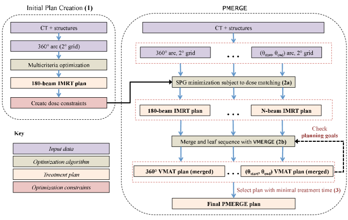
Figure 1: Illustration of our three step process. 1) An initial IMRT plan is created to generate a set of dose constraints for pmerge. 2a) pmerge uses these constraints to generate a set of partial-arc solutions. 2b) Each $N$-beam partial-arc solution is merged and sequenced with vmerge, subject to the user-defined planning goals. 3) The final plan is selected as the one with the lowest treatment time.

2.1 Delivery parameters and leaf sequencing

There are two classes of methods for solving VMAT problems: one-stage and two-stage [Yu2011]. In the one stage method, known as direct aperture optimization, the paths of the MLC leaves are directly optimized, taking into account limitations of finite leaf speed. Instead, we use a two-stage planning approach to solve the VMAT problem for any size arc. In the first step, an $N$-beam IMRT problem with beams spaced every $2^{\circ}$ is solved to generate a set of $N$ fluence maps ($f^{1}_{l,x}$, $f^{2}_{l,x}$…, $f^{N}_{l,x}$), where each fluence map is a K$\times$L matrix of $L$ rows of MLC leaves and $K$ columns. In the second step, a leaf sequencing algorithm determines the MLC leaf trajectories, gantry speed ($\omega$), and dose rate ($r$) for each 2^∘ arc portion, which we call a gantry sector. In leaf sequencing, the trajectories of the leaves are set so that the accumulated fluence over a given gantry sector matches the input fluence from the static beam fluence map. To accomplish this, we employ a widely used dynamic MLC (dMLC) sequencer which creates a “sliding window” that moves leaves unidirectionally across the field for each arc portion [Spirou1994, Svensson1994]. Thus, for each gantry sector, the leaves must move from left-to-right (or right-to-left), traversing the entire field of width $W$. In practice, the gantry speed, dose rate and maximum leaf speed are constrained by the limitations of the linac hardware and will have a significant effect on the total treatment time [Boylan2011]. We select a set of hardware capabilities (Table 1) that are representative of the values found on many current treatment machines.

Table 1: VMAT delivery parameters and constraints

• Delivery parameter	Symbol	Constraint
  Maximum leaf speed	$v_{\max}$	2.5 cm/s
  Maximum gantry speed	$\omega_{\max}$	6 deg/s
  Minimum gantry speed	$\omega_{\min}$	0 deg/s
  Maximum dose rate	$r_{\max}$	600 MU/min
  Minimum dose rate	$r_{\min}$	50 MU/min

When applied to VMAT, the total treatment time using the dMLC algorithm is controlled by three terms: 1) the total distance the leaves must travel during delivery, 2) the amount of beam modulation required to deliver the desired fluence map and 3) the maximum gantry speed. These three considerations can be combined to provide an equation to calculate the total treatment time for a plan with $N$ gantry sectors of arc lengths $\Delta\theta_{i}$:

$$T=\displaystyle\sum_{i=1}^{N}\max\left[\frac{W}{v_{\max}}+\frac{\displaystyle\max_{\mbox{rows$\;l$}}\left[\displaystyle\sum_{x=1}^{K}\left(\frac{\mbox{d}f_{l,x}^{i}(x)}{\mbox{d}x}\right)^{+}\right]}{r_{i}},\frac{\Delta\theta_{i}}{\omega_{\max}}\right]$$ (1)

where the (.)⁺ operator is shorthand for $\max\left(0,.\right)$. The first term in (1) is the field width divided by the maximum leaf speed, which is the minimum time required for the leaves to move from the left side of the field to the right (or vice versa) if no fluence were delivered. As fluence is added, the leaf speed will be modulated to allow enough time for the dose to accumulate. This time is described in the second term as the sum-of-positive gradients (SPG), a measure of the amount of variation in a field [Craft2007a], divided by the dose rate. Fields that are highly varied (have a high SPG term) will take longer to deliver with dMLC. Finally, because of limitations on the maximum gantry speed, the time required to deliver a gantry sector cannot be less than time required to move the gantry at maximum speed over the gantry sector. The total treatment time is the sum of the time required to deliver each of the $N$ gantry sectors.

Given a fixed set of hardware capabilities, the total treatment time can be improved by either decreasing the total number of gantry sectors $N$ or by decreasing the SPG. Decreasing the number of gantry sectors motivates the partial-arc strategy described here, and the merging strategy vmerge – by using partial-arc solutions, we begin with a lower number of fluence maps than in a full arc, and this is decreased further by combing gantry sectors in the merging routine. Thus, for each gantry sector that is merged or eliminated with a partial-arc, the treatment time decreases by no less than $W/v_{\max}$. Finally, to further reduce treatment time, we incorporate SPG minimization into our optimization step as described in Section 2.3.

2.2 Initial plan optimization

We use a multicriteria optimization (MCO) approach to solve the initial 180-beam IMRT problem, as described in Craft2012. Briefly, in MCO, each structure is assigned an objective function, and a tradeoff surface of Pareto optimal plans is generated by the optimizer [Monz2008, Thieke2007]. A Pareto optimal plan is one where no improvements could be made to any objective without worsening another objective [cotrutz2001]. The user navigates this tradeoff surface and selects the plan that best meets the treatment goals.

The general multicriteria IMRT formulation is the following:

optimize $$\{g_{1}(d),~{}g_{2}(d),\ldots g_{M}(d)\}$$

subject to $$d=Df$$

$$d\in C$$

$$f\geq 0$$ (2)

where $g_{i}$ are the $M$ objective functions describing the dose to a particular structure (e.g., mean dose to stomach), $d$ is the vector of voxel doses, $D$ is the dose-influence matrix, and $f$ is a concatenation of all the fluence maps into a single beamlet fluence vector. The set $C$ is a convex set of dose constraints (e.g. maximum dose to the target) that are designed to be met by all plans. We use the CERR 3.0 [deasy2003] environment and its beamlet based quadratic infinite beam (QIB) dose computation to calculate the dose influence matrix, with a computation time of around 10 minutes per case. Given a dose matrix, the dose distribution can be calculated from the fluence maps in seconds.

The constraints on the planning target volumes (PTV) and the OARs for each site are listed in Table 2. In our MCO formulation, we had the optimizer minimize the mean doses to the OARs. Additionally, we include as an OAR unclassified tissue (u.t.), which encompasses all voxels that do not belong to another structure. Optimizations are performed using the solver described by Chen2010. We then choose a plan for each treatment site by exploring the Pareto surface and selecting a plan that balanced the dose the OARs.

Table 2: Target coverage constraints and OAR list used in the MCO optimization

Treatment site	PTV Min; Max (Gy)	OARs
Lung	50.0; 55.0	left lung, right lung, esophagus,
		heart, spinal cord, u.t.
Liver	50.0; 55.0	left lung, right lung, liver, spinal cord,
		stomach, left kidney, right kidney, u.t.
Prostate	79; 85.3	left femoral head, right femoral head,
		anterior rectum, bladder, u.t.

2.3 Generating the partial-arc plans

The set of partial-arc solutions are created by iteratively solving the $2^{\circ}$ grid IMRT problem for a range of partial-arcs. In creating the plans, we respect the constraint that the gantry cannot rotate through $0^{\circ}$, a line from the couch to the floor. Plans are created with arc lengths every 40^∘ ($360^{\circ},320^{\circ}$, …) until there are no feasible solutions. For each arc length, plans are created with arcs centered at intervals of $40^{\circ}$. Thus, there is one $360^{\circ}$ plan, three $320^{\circ}$ degree plans (beginning at $-40^{\circ},0^{\circ},40^{\circ}$), five $280^{\circ}$ plans, etc.

Each partial-arc solution is created to maintain the same dose quality as the initial 180-beam solution. This is done with the same solver used to solve the original 180-beam MCO formulation, except run in feasibility mode, where the solver returns the first solution it finds which satisfies all of the hard constraints. Because treatment time scales with the complexity of the solution, this solution is then smoothed using total SPG as the objective function, while maintaining dosimetric feasibility:

SPG minimization subject to dose matching

minimize $$\sum_{i=1}^{N}\max_{\mbox{rows$\;l$}}\left[\displaystyle\sum_{x=1}^{K}\left(\frac{\mbox{d}f_{l,x}^{i}(x)}{\mbox{d}x}\right)^{+}\right]$$

subject to $$d=Df$$

$$d_{i}\geq B_{L},~{}\forall i\in\hbox{~{}target}$$

$$d_{i}\leq B_{U},~{}\forall i$$

$$\mbox{mean}_{j}^{(P)}(d)\leq\hbox{mean}^{(I)}_{j}(d),~{}\forall\hbox{~{}OAR}\;j$$

$$f\geq 0$$ (3)

where $B_{L}$ and $B_{U}$ is the target lower bound, $B_{U}$ is the upper bound on the dose, and $\hbox{mean}^{(P)}_{j}(d)$ and mean${}_{j}^{(I)}(d)$ are the mean doses to the $j$th OAR for the partial-arc and initial plans, respectively. This formulation ensures that for each partial-arc solution the target coverage is no less than, and the maximum dose and the mean doses to each OAR are no greater than those of the initial plan.

2.4 Merging and final plan selection

After the SPG minimization step, we have a set of IMRT solutions for various partial-arcs. To improve the delivery efficiency, we use a previously described fluence map merging strategy called vmerge to combine gantry sectors [Craft2012]. Briefly, vmerge employs a greedy merging strategy to iteratively add similar neighboring fluence maps – for each iteration, the two neighboring fluence maps that are most similar are added together into a single fluence map. This reduces the number of gantry sectors and improves the delivery efficiency, at the expense of reducing the amount of fluence modulation and the angular resolution.

pmerge automates vmerge by utilizing a quality cutoff, which limits how much the dose can change, and automatically stops merging when the quality drops below the planning goals. Here, the planner is free to chose how much the dose quality is allowed to change in order to improve delivery efficiency. We use the initial high-quality plan as a guide for how to set these goals. For the OARs that receive the most radiation, we limit the partial-arc mean dose to less than 105% of the initial mean dose for that OAR. Additionally, we ensure that the target coverage stays above 98%, and the maximum dose is less than 102% of the initial maximum dose. Finally, we illustrate the use of site-specific planning goals, including limiting the maximum dose to the femoral heads in the prostate case and adding additional constraints on the left lung dose in the lung case. The full sets of planning goals are provided in Tables 3-5.

3 Results

3.1 Lung

Table 3: Lung: Planning goals, dose quality and treatment times

	Goal	Initial (I)	pmerge (P)
u.t. dose	$\hbox{mean}^{(P)}_{UT}<1.10\times\hbox{mean}^{(I)}_{UT}$	2.8 Gy	3.0 Gy
Right lung	$\hbox{mean}^{(P)}_{RL}<1.05\times\hbox{mean}^{(I)}_{RL}$	0.6 Gy	0.5 Gy
Left lung	${}^{\dagger}V40^{(P)}<1.05\times V40^{(I)}$	9.4%	9.5%
	$V50^{(P)}<1.05\times V50^{(I)}$	3.0%	3.0%
Target coverage	$V50^{(P)}>0.98\times V50^{(I)}$	100%	98.2%
Maximum dose	$\max^{(P)}<1.02\times\max^{(I)}$	55.0 Gy	55.8 Gy
(Start, end) angles		(0∘, 360∘)	(60∘, 260∘)
Treatment time‡		211 s	127 s
${\dagger}$V$x$ denotes the volume receiving at least $x$ Gy
${\ddagger}$Treatment times are after merging

We navigate to an initial 180-beam plan with mean doses and target coverage as shown in Table 3. The treatment time of the initial plan before merging is 771 s, and is reduced to 211 s with vmerge. The initial plan and vmerge plans are shown with the outer two rings of Fig 2(c). The vmerge plan is notable for a large arc portion of $116^{\circ}$ on the contralateral side of the PTV where the gantry speed is at its maximum. As shown in Figure 2(d), there is little fluence delivered over this section in the initial 180-beam plan.

Partial-arc solutions were attempted for arcs with lengths between $80^{\circ}$ and $360^{\circ}$, at intervals of $40^{\circ}$. 50 had feasible solutions that met the dose constraints from Equation 3, and 26 of these had lower treatment times than the vmerge plan. The final pmerge plan has an arc length of $200^{\circ}$ and treatment time of 127 s, and is shown in the inner two rings of Fig 2c, both before and after merging. The total difference in treatment times between the vmerge (211 s) and pmerge (127 s) plans is 84 s, a 40% reduction. Optimization, merging and sequencing took about 40 minutes to complete all 64 plans, running in parallel on 8 processors. Computation time was similar across the lung, liver and prostate cases.

3.2 Liver

Table 4: Liver: Planning goals, dose quality and treatment times

	Goal	Initial (I)	pmerge (P)
u.t.	$\hbox{mean}^{(P)}_{UT}<1.10\times\hbox{mean}^{(I)}_{UT}$	5.7 Gy	5.6 Gy
Right lung	$\hbox{mean}^{(P)}_{RL}<1.05\times\hbox{mean}^{(I)}_{RL}$	9.1 Gy	9.2 Gy
Left lung	no constraint (mean${}_{LL}^{(P)})$	1.5	1.5 Gy
Liver	$\hbox{mean}^{(P)}_{L}<1.05\times\hbox{mean}^{(I)}_{L}$	23.3 Gy	23.3 Gy
Right kidney	$\hbox{mean}^{(P)}_{RK}<1.05\times\hbox{mean}^{(I)}_{RK}$	5.8 Gy	4.7 Gy
Left kidney	no constraint (mean${}_{LK}^{(P)})$	0.7 Gy	0.4 Gy
Target coverage	$V50^{(P)}>0.98\times V50^{(I)}$	100%	98.0%
Maximum dose	$\max^{(P)}<1.02\times\max^{(I)}$	55.0 Gy	55.6 Gy
(Start, end) angles		(0∘, 360∘)	(100∘, 340∘)
Treatment time†		357 s	245 s
${\dagger}$Treatment times are after merging

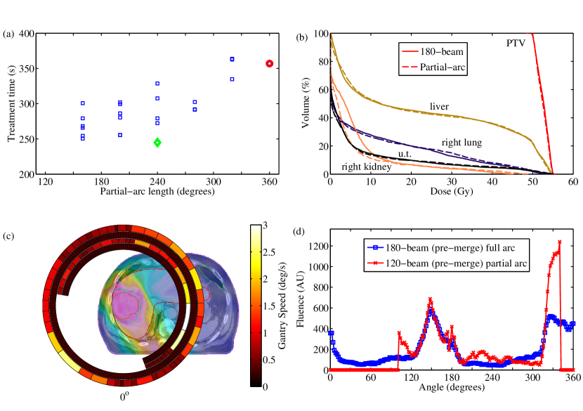
Figure 3: Liver: a) Final treatment times for each of the merged partial-arc plans (blue squares) with treatment times near or below the vmerge plan (red circle). b) DVH for the initial 180-beam plan (solid) and the pmerge plan (dashed). c) Initial and merged gantry sectors for the pmerge plan (inner rings) and 180-beam plan (outer rings) over the pmerge dose wash. d) Distribution of fluence for the initial solution and the optimal partial-arc before merging (120-beam).

We navigate to an original 180-beam solution with mean OAR doses, target coverage and maximum dose as shown in Table 4. The treatment time before merging for the full arc solution is 1214 s and is reduced to 357 s with vmerge (Figure 3(c), outer rings). Partial-arc solutions were attempted for arcs lengths between $80^{\circ}$ and $360^{\circ}$, at intervals of $40^{\circ}$, and 33 had feasible solutions. There were no solutions with arc lengths less than $160^{\circ}$. Of the feasible partial-arcs, 19 had lower treatment times than the vmerge plan.

The selected partial-arc has an arc length of $240^{\circ}$ (Figure 3(c), inner rings) and treatment time of 245 s. The total difference in treatment times between the vmerge plan (357 s) and pmerge plan (245 s) is 112 s, a 31% reduction. In this case the initial 180-beam solution is significant for two peaks of fluence, one at approximately $150^{\circ}$ and one at $330^{\circ}$, as shown in Figure 3(d). The optimal partial-arc includes both of these peaks, and is able to eliminate the first $100^{\circ}$ where the amount of required fluence is low.

3.3 Prostate

Table 5: Prostate: Planning goals, dose quality and treatment times

	Goal	Initial (I)	pmerge (P)
u.t.	$\hbox{mean}^{(P)}_{UT}<1.10\times\hbox{mean}^{(I)}_{UT}$	15.5 Gy	16.4 Gy
Anterior rectum	$\hbox{mean}^{(P)}_{AR}<1.05\times\hbox{mean}^{(I)}_{AR}$	41.4 Gy	41.8 Gy
Bladder	$\hbox{mean}^{(P)}_{B}<1.05\times\hbox{mean}^{(I)}_{B}$	39.6 Gy	39.8 Gy
Left femoral head	$\max^{(P)}_{LFH}<1.10\times\max^{(I)}_{LFH}$	33.6 Gy	35.5 Gy
Right femoral head	$\max^{(P)}_{RFH}<1.10\times\max^{(I)}_{RFH}$	37.0 Gy	38.3 Gy
Target coverage	$V79^{(P)}>0.98\times V79^{(I)}$	100%	98.2%
Maximum dose	$\max^{(P)}<1.02\times\max^{(I)}$	85.3 Gy	86.7 Gy
(Start, end) angles		(0∘, 360∘)	(40∘, 320∘)
Treatment time†		178 s	147 s
${\dagger}$Treatment times are after merging

We navigated to an original 180-beam solution with mean OAR doses, target coverage and maximum dose as shown in Table 5. The treatment time before merging for the full arc solution is 860 s and is reduced to 178 s with vmerge (Figure 4(c), outer two rings). Unlike the lung and liver cases, the vmerge plan has regularly spaced arc portions of similar size, and the fluence is delivered fairly uniformly around the target, as shown in Figure 4(d). This is reflected in the optimal partial-arc solution, which is highly similar to the initial plan through nearly the full arc.

Partial-arc solutions were created for arcs lengths between $80^{\circ}$ and $360^{\circ}$, at intervals of $40^{\circ}$, and 45 had feasible solutions. Of the 45, only 3 had treatment times lower than the vmerge plan. There were no feasible partial-arcs at $80^{\circ}$. For plans with arc lengths of less than 280^∘, almost no merging was possible before the plan quality degraded beyond the stopping criteria. The selected partial-arc has an arc length of $300^{\circ}$ (Figure 4(c), inner rings) and treatment time of 147 s. The total difference in treatment times between the vmerge (178 s) plan and pmerge plan (147 s) is 31 s, a 17% reduction.

4 Discussion and conclusions

We present a method for automatically creating efficient VMAT partial-arc plans from a high quality reference plan. By sampling a set of partial-arcs, we reduced treatment times for a lung, liver and prostate case. The final pmerge plans reflect the underlying geometry of the problem. For the lung and liver cases with non-centralized PTVs, a signifiant portion of the full-arc can be eliminated with little effect on the dose quality. This allowed for the treatment time to be reduced by 40% and 31% respectively. The reduction in treatment time for the prostate case was more modest at 17%. As might be expected for a centrally located target, the fluence was distributed more evenly around the arc, and most of the partial-arcs were not able to improve the delivery efficiency while maintaining the dose quality to within the specified boundaries.

In pmerge, the dose quality of the final partial-arc is designed to be highly similar to the initial plan. However, the pmerge plan is limited only by the planning goals specified after the initial plan creation. Thus, the partial-arc plan could deviate from the initial plan in ways that are not specified by this quality threshold. Any number or type of constraints could easily be imposed on the final solution to ensure that the initial plan and pmerge plan were sufficiently similar. In practice, we did not find that it was necessary to impose many constraints in order to match the solutions. Although we were free to use any number of dose-volume points or EUD functions, our planning goals were restricted to only one or two constraints per OAR, usually a limit on the mean or maximum dose. For all three cases, these were sufficient to closely match the doses across the DVH, even for OARs which were not explicitly specified.

In VMAT, as in IMRT, there are many different ways to deliver the fluence that will give highly similar dose distributions. Because the treatment time is dependent on the geometry of these fluence maps, the method by which the initial fluence maps are created is an important determinant of treatment time. Although pmerge is not confined to any single optimization strategy, we found that using SPG smoothing was critically important to achieving highly efficient plans. Indeed, fluence map smoothing is important in IMRT (e.g.  [Matuszak2008]), where it is know that the complexity of the fluence maps – and hence the number of monitor units – can be greatly reduced without significantly impacting the dose distribution.

Although the partial-arc global search can be parallelized, we recognize that the high computation time is a limit to our method. The observation that the optimizer distributes fluence very similarly between the full-arc and partial-arc plans suggests a way of approximating the appropriate partial-arc without having to enumerate all of the possibilities. One strategy would be to plot the arrangement of fluence around the arc and have the planner select the partial-arc that captures the critical angles. For the lung and liver cases, we find that there were many different partial-arcs that greatly improved the treatment time, and thus it is not essential to find the absolute global minimum when plans near the minimum are almost equivalent (see Figures 2(a) and 3(a)). More importantly, we conclude that partial-arcs that cover certain critical angles are useful for reducing treatment time in VMAT, and pmerge is a useful first-pass method at finding the optimal plan.

References

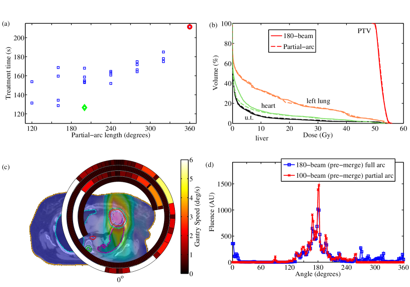
Figure 2: Lung: a) Final treatment times for each of the merged partial-arc plans (blue squares) with treatment times near or below the vmerge plan (red circle). b) DVH for the initial 180-beam plan (solid) and the pmerge plan (dashed). c) Initial and merged gantry sectors for the pmerge plan (inner rings) and 180-beam plan (outer rings) over the pmerge dose wash. d) Distribution of fluence for the initial solution and the optimal partial-arc before merging (100-beam).

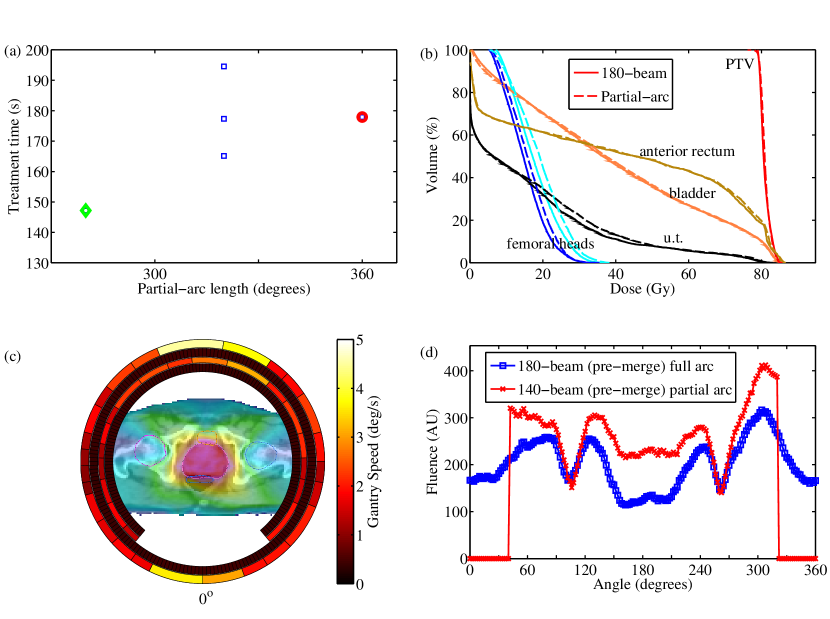
Figure 4: Prostate: a) Final treatment times for each of the merged partial-arc plans (blue squares) with treatment times near or below the vmerge plan (red circle). b) DVH for the initial 180-beam plan (solid) and the pmerge plan (dashed). c) Initial and merged gantry sectors for the pmerge plan (inner rings) and 180-beam plan (outer rings) over the pmerge dose wash. d) Distribution of fluence for the initial solution and the optimal partial-arc before merging (140-beam).

References

- [1] \harvarditemBedford2009Bedford2009 Bedford J 2009 Medical Physics 36, 5128–5138.
- [2] \harvarditemBertelsen et al.2011Bertelsen2011 Bertelsen A, Lorenzen E \harvardand Brink C 2011 Medical Physics 38, 4802–4810.
- [3] \harvarditemBese et al.2007Bese2007 Bese N, Hendry J \harvardand Jeremic B 2007 International Journal of Radiation Oncology Biology Physics 68(3), 654–661.
- [4] \harvarditemBortfeld \harvardand Webb2009Bortfeld2009 Bortfeld T \harvardand Webb S 2009 Physics in Medicine and Biology 54, N9–N20.
- [5] \harvarditemBoylan et al.2011Boylan2011 Boylan C, Rowbottom C \harvardand Mackay R 2011 Physics in Medicine and Biology 56, 4119–4133.
- [6] \harvarditemChen et al.2010Chen2010 Chen W, Craft D, Madden T, Zhang K, Kooy H \harvardand Herman G 2010 Medical Physics 37, 4938–4945.
- [7] \harvarditemClivio et al.2009Clivio2009 Clivio A, Fogliata A, Franzetti-Pellanda A, Nicolini G, Vanetti E, Wyttenbach R \harvardand Cozzi L 2009 Radiotherapy and Oncology 92(1), 118–124.
- [8] \harvarditemCotrutz et al.2001cotrutz2001 Cotrutz C, Lahanas M, Kappas C \harvardand Baltas D 2001 Physics in Medicine and Biology 46, 2161.
- [9] \harvarditemCozzi et al.2008Cozzi2008 Cozzi L, Dinshaw K, Shrivastava S, Mahantshetty U, Engineer R, Deshpande D, Jamema S, Vanetti E, Clivio A, Nicolini G et al. 2008 Radiotherapy and Oncology 89(2), 180–191.
- [10] \harvarditemCraft et al.2012Craft2012 Craft D, McQuaid D, Wala J, Chen W, Salari E \harvardand Bortfeld T 2012 Medical Physics 39(2), 686–696.
- [11] \harvarditemCraft et al.2007Craft2007a Craft D, Süss P \harvardand Bortfeld T 2007 International Journal of Radiation Oncology Biology Physics 67(5), 1596–1605.
- [12] \harvarditemDeasy et al.2003deasy2003 Deasy J, Blanco A \harvardand Clark V 2003 Medical Physics 30, 979–985.
- [13] \harvarditemGuckenberger et al.2009Guckenberger2009 Guckenberger M, Richter A, Krieger T, Wilbert J, Baier K \harvardand Flentje M 2009 Radiotherapy and Oncology 93(2), 259–265.
- [14] \harvarditemHall \harvardand Wuu2003Hall2003 Hall E \harvardand Wuu C 2003 International Journal of Radiation Oncology Biology Physics 56(1), 83–88.
- [15] \harvarditemHoogeman et al.2008Hoogeman2008 Hoogeman M, Nuyttens J, Levendag P \harvardand Heijmen B 2008 International Journal of Radiation Oncology Biology Physics 70(2), 609–618.
- [16] \harvarditemJohnston et al.2011Johnston2011 Johnston M, Clifford S, Bromley R, Back M, Oliver L \harvardand Eade T 2011 Clinical Oncology 23, 503–511.
- [17] \harvarditemKry et al.2005Kry2005 Kry S, Salehpour M, Followill D, Stovall M, Kuban D, White R \harvardand Rosen I 2005 International Journal of Radiation Oncology Biology Physics 62(4), 1195–1203.
- [18] \harvarditemLuan et al.2008Luan2008 Luan S, Wang C, Cao D, Chen D, Shepard D, Yu C et al. 2008 Medical Physics 35(1), 61–69.
- [19] \harvarditemMatuszak et al.2008Matuszak2008 Matuszak M, Larsen E, Jee K, McShan D \harvardand Fraass B 2008 Medical Physics 35, 1532–1546.
- [20] \harvarditemMonz et al.2008Monz2008 Monz M, Küfer K, Bortfeld T \harvardand Thieke C 2008 Physics in Medicine and Biology 53, 985–998.
- [21] \harvarditemOtto2008Otto2008 Otto K 2008 Medical Physics 35, 310–317.
- [22] \harvarditemPalma et al.2008Palma2008 Palma D, Vollans E, James K, Nakano S, Moiseenko V, Shaffer R, McKenzie M, Morris J \harvardand Otto K 2008 International Journal of Radiation Oncology Biology Physics 72(4), 996–1001.
- [23] \harvarditemRangaraj et al.2010Rangaraj2010 Rangaraj D, Oddiraju S, Sun B, Santanam L, Yang D, Goddu S \harvardand Papiez L 2010 Medical Physics 37, 4056–4067.
- [24] \harvarditemRao et al.2010Rao2010 Rao M, Yang W, Chen F, Sheng K, Ye J, Mehta V, Shepard D \harvardand Cao D 2010 Medical Physics 37, 1350–1359.
- [25] \harvarditemRuben et al.2008Ruben2008 Ruben J, Davis S, Evans C, Jones P, Gagliardi F, Haynes M \harvardand Hunter A 2008 International Journal of Radiation Oncology Biology Physics 70(5), 1530–1536.
- [26] \harvarditemSpirou \harvardand Chui1994Spirou1994 Spirou S \harvardand Chui C 1994 Medical Physics 21, 1031–1041.
- [27] \harvarditemSvensson et al.1994Svensson1994 Svensson R, Kallman P \harvardand Brahme A 1994 Physics in Medicine and Biology 39, 37–61.
- [28] \harvarditemTeoh et al.2011Teoh2011 Teoh M, Clark C, Wood K, Whitaker S \harvardand Nisbet A 2011 British Journal of Radiology 84(1007), 967–996.
- [29] \harvarditemThieke et al.2007Thieke2007 Thieke C, Küfer K, Monz M, Scherrer A, Alonso F, Oelfke U, Huber P, Debus J \harvardand Bortfeld T 2007 Radiotherapy and Oncology 85(2), 292–298.
- [30] \harvarditemWang et al.2003Wang2003 Wang J, Li X, D’Souza W \harvardand Stewart R 2003 International Journal of Radiation Oncology Biology Physics 57(2), 543–552.
- [31] \harvarditemYu \harvardand Tang2011Yu2011 Yu C \harvardand Tang G 2011 Physics in Medicine and Biology 56, R31–R54.
- [32] \harvarditemZhang et al.2010Zhang2010b Zhang P, Happersett L, Hunt M, Jackson A, Zelefsky M \harvardand Mageras G 2010 International Journal of Radiation Oncology Biology Physics 76(5), 1456–1462.
- [33]