Minimal lepton flavor violating realizations
of minimal seesaw models

D. Aristizabal Sierraa,111e-mail address: daristizabal@ulg.ac.be, A. Degeea,222e-mail address: audrey.degee@ulg.ac.be, J. F. Kamenikb,c,333e-mail address: jernej.kamenik@ijs.si

aIFPA, Dep. AGO, Universite de Liege,
Bat B5, Sart Tilman B-4000 Liege 1, Belgium
.

bJ. Stefan Institute,
Jamova 39, P. O. Box 3000, 1001 Ljubljana, Slovenia
.

cDepartment of Physics, University of Ljubljana,
Jadranska 19, 1000 Ljubljana, Slovenia
.

We study the implications of the global U(1)R𝑈subscript1𝑅U(1)_{R} symmetry present in minimal lepton flavor violating implementations of the seesaw mechanism for neutrino masses. In the context of minimal type I seesaw scenarios with a slightly broken U(1)R𝑈subscript1𝑅U(1)_{R}, we show that, depending on the R𝑅R-charge assignments, two classes of generic models can be identified. Models where the right-handed neutrino masses and the lepton number breaking scale are decoupled, and models where the parameters that slightly break the U(1)R𝑈subscript1𝑅U(1)_{R} induce a suppression in the light neutrino mass matrix. We show that within the first class of models, contributions of right-handed neutrinos to charged lepton flavor violating processes are severely suppressed. Within the second class of models we study the charged lepton flavor violating phenomenology in detail, focusing on μeγ𝜇𝑒𝛾\mu\to e\gamma, μ3e𝜇3𝑒\mu\to 3e and μe𝜇𝑒\mu-e conversion in nuclei. We show that sizable contributions to these processes are naturally obtained for right-handed neutrino masses at the TeV scale. We then discuss the interplay with the effects of the right-handed neutrino interactions on primordial BL𝐵𝐿B-L asymmetries, finding that sizable right-handed neutrino contributions to charged lepton flavor violating processes are incompatible with the requirement of generating (or even preserving preexisting) BL𝐵𝐿B-L asymmetries consistent with the observed baryon asymmetry of the Universe.

1 Introduction

The observation of neutrino flavor oscillations constitutes an experimental proof of lepton flavor violation [1]. In principle, other manifestations of such effects could be expected to show up in the charged lepton sector as well. However, the lack of a definitive model for neutrino mass generation implies that conclusive predictions for lepton flavor violating processes can not be made, and even assuming a concrete model realization for neutrino masses, predictions for such effects can only be done if the flavor structure of the corresponding realization is specified.

A problem that one faces when dealing with charged lepton flavor violating phenomenology is related with the arbitrariness of the free parameters that define these observables. In this regards the minimal lepton flavor violation (MLFV) hypothesis [5, 6, 7, 8] is a very useful guide for constructing predictive models in which lepton violating signals are entirely determined by low-energy neutrino data. The relationship between the free parameters and neutrino observables can arise via either a restrictive MLFV hypothesis or in some cases due to the intrinsic structure of the corresponding model (whenever the number of free parameters is comparable to the number of neutrino observables).

In the canonical seesaw (type-I) the kinetic sector of the model is invariant under a global large flavor symmetry group GF=SU(3)e×SU(3)×SU(3)Nsubscript𝐺𝐹𝑆𝑈subscript3𝑒𝑆𝑈subscript3𝑆𝑈subscript3𝑁G_{F}=SU(3)_{e}\times SU(3)_{\ell}\times SU(3)_{N}, where \ell, e𝑒e and N𝑁N denote triplets in flavor space constructed from the electroweak lepton doublets and singlets and RH neutrinos. In addition there is an invariance under an extra global U(1)R𝑈subscript1𝑅U(1)_{R} [4, 8]. In principle the charges associated with this global transformation (hereafter denoted by R𝑅R) are arbitrary, and thus different R𝑅R-charge assignments define different models with their own consequences for lepton flavor violating phenomenology. In particular, models for which the R𝑅R charges allow for large Yukawa couplings and TeV RH neutrino masses should lead to sizable charged lepton flavor violating processes.

Consistent models of 𝒪(TeV)𝒪TeV{\cal O}(\mbox{TeV}) RH states and large Yukawa couplings are achievable if cancellations among different pieces of the light neutrino mass matrix are allowed, and the RH neutrino mass spectrum is not strongly hierarchical [9]111In the case of a large hierarchy among the different RH neutrino masses the one-loop finite corrections to the light neutrino mass matrix can exceed the corresponding tree-level contributions. Neglecting such corrections can in this case lead to a model inconsistent with neutrino data  [10].. The class of TeV scale seesaw models arising from the presence of the U(1)R𝑈subscript1𝑅U(1)_{R} symmetry are expected to be in that sense different: no cancellations are needed because the suppression in the effective light neutrino mass matrix is no longer constrained to be related with the heaviness of the RH neutrinos.

In this paper we study the implications of a slightly broken U(1)R𝑈subscript1𝑅U(1)_{R} symmetry in minimal type-I seesaw models (with two RH neutrinos) 222Models with an arbitrary number of RH neutrinos were considered for the first time in [11]. 333For related discussion within Type III and mixed Type I+III seesaw scenarios c.f. [12].. We show that the intrinsic structure of the relevant models leads to a flavor pattern completely determined by low-energy neutrino observables, thus realizing in that way the MLFV hypothesis. This feature in addition to a slightly broken U(1)R𝑈subscript1𝑅U(1)_{R} leads to sizable μeγ𝜇𝑒𝛾\mu\to e\gamma, μ3e𝜇3𝑒\mu\to 3e and μe𝜇𝑒\mu-e processes. This is in contrast to models where U(1)L𝑈subscript1𝐿U(1)_{L} is slightly broken so that lepton number and lepton flavor violation occur at the same scale.

In models with slightly broken lepton number it has been shown that leptogenesis is reconcilable with large charged lepton flavor violating rates, as the washouts induced by the RH neutrino states are controlled by the amount of lepton number violation [13]. We show however, that in the class of models considered here this statement does not hold, and that indeed leptogenesis and sizable charged lepton flavor violating effects are mutually exclusive. However, since both phenomena cover non-overlapped regions of parameter space their analyses are complementary. We therefore also explore the constraints on these models derived from the requirement of not erasing—via the RH neutrino dynamics—a preexisting BL𝐵𝐿B-L asymmetry below the value consistent with the observed baryon asymmetry of the Universe.

The rest of this paper is organized as follows: in section 2 we discuss in detail the scenarios arising from the different R𝑅R-charge assignments. In section 3 we discuss the phenomenology of charged lepton flavor violating decays in the representative models. In section 4 we analyze the implications of such constructions for scenarios of high scale baryogenesis by quantifying—via the Boltzmann equations—the effects of the RH neutrino dynamics on preexisting BL𝐵𝐿B-L asymmetries. In section 5 we present our conclusions and final remarks. Explicit formulas used in the calculation of the different lepton flavor violating processes under study are given in appendix A.

2 The setups

The kinetic and gauge interaction Lagrangian of the standard model extended with two RH neutrinos exhibits a global G=U(3)e×U(3)×U(2)N𝐺𝑈subscript3𝑒𝑈subscript3𝑈subscript2𝑁G=U(3)_{e}\times U(3)_{\ell}\times U(2)_{N} symmetry. Factorizing three U(1)𝑈1U(1) factors from G𝐺G, the global symmetry can be rewritten as U(1)Y×U(1)L×U(1)R×GF𝑈subscript1𝑌𝑈subscript1𝐿𝑈subscript1𝑅subscript𝐺𝐹U(1)_{Y}\times U(1)_{L}\times U(1)_{R}\times G_{F} where U(1)Y,L𝑈subscript1𝑌𝐿U(1)_{Y,L} can be identified with global hypercharge and lepton number whereas the U(1)R𝑈subscript1𝑅U(1)_{R} is a “new” global symmetry [4, 8]. The remaining direct product group GF=SU(3)e×SU(3)×SU(2)Nsubscript𝐺𝐹𝑆𝑈subscript3𝑒𝑆𝑈subscript3𝑆𝑈subscript2𝑁G_{F}=SU(3)_{e}\times SU(3)_{\ell}\times SU(2)_{N} determines the flavor symmetry which is explicitly broken in the Yukawa sector.

In minimal lepton flavor violating seesaw models the Yukawa (mass) matrices are treated as spurion fields transforming under GFsubscript𝐺𝐹G_{F} in such a way that the corresponding Yukawa (mass) terms in the leptonic Lagrangian remain invariant under the global flavor symmetry. The usual procedure is then based on an effective theory approach in which a set of non-renormalizable effective operators are constructed from the spurions.444An exception are the explicit MLFV models discussed in Ref. [7]. With the operators at hand and under certain restrictions on GFsubscript𝐺𝐹G_{F} the lepton flavor violating effects can be estimated by means of low-energy neutrino data [5, 8]. Here, instead, we explicitly consider the seesaw Lagrangian with a slightly broken U(1)R𝑈subscript1𝑅U(1)_{R} and classify the possible realizations according to the R𝑅R-charge assignments. Under this consideration, in the models featuring sizable lepton flavor violating effects, the flavor structure is determined by low-energy observables as well (up to a global normalization factor), not as a consequence of a restricted MLFV hypothesis but by the intrinsic structure of the resulting models.

Depending on the R𝑅R-charge assignments two classes of generic models can be identified. Let us discuss this in more detail. Requiring U(1)R𝑈subscript1𝑅U(1)_{R} invariance of the charged lepton Yukawa terms determines R(e)𝑅𝑒R(e) in terms of R(,H)𝑅𝐻R(\ell,H). After fixing R(H)=0𝑅𝐻0R(H)=0, to avoid charging the quark sector, the remaining charges can be fixed by starting with R(N1,2)𝑅subscript𝑁12R(N_{1,2}). In order to have sizable lepton flavor violating effects both the N1,2subscript𝑁12N_{1,2} Majorana mass terms should be suppressed by R𝑅R-breaking parameters (generically denoted by ϵitalic-ϵ\epsilon), so R(N1,2)0𝑅subscript𝑁120R(N_{1,2})\neq 0. Thus one has only three possibilities: (A) R(N1)=R(N2)𝑅subscript𝑁1𝑅subscript𝑁2R(N_{1})=R(N_{2}), (B) R(N1)=R(N2)𝑅subscript𝑁1𝑅subscript𝑁2R(N_{1})=-R(N_{2}) and (C) |R(N1)||R(N2)|𝑅subscript𝑁1𝑅subscript𝑁2|R(N_{1})|\neq|R(N_{2})|. The phenomenology of case (C), however, is expected to be similar to the one arising from models with R𝑅R-charge assignments of type (A). The reason being that in that case the N1N2subscript𝑁1subscript𝑁2N_{1}-N_{2} mixing is always U(1)R𝑈subscript1𝑅U(1)_{R} suppressed, which in turn implies suppressed charged lepton flavor violating processes (equivalently, the effective neutrino mass matrix will not be ϵitalic-ϵ\epsilon suppressed, forcing tiny Yukawas or heavy N1,2subscript𝑁12N_{1,2} states). This is to be compared with models based on R𝑅R-charge assignments of type (B), where the N1N2subscript𝑁1subscript𝑁2N_{1}-N_{2} turns out to be maximal and a set of unsuppressed N𝑁\ell-N Yukawa couplings can be always obtained by properly chosing R()𝑅R(\ell) (in these models the effective neutrino mass matrix involves extra ϵitalic-ϵ\epsilon suppression factors).

In summary depending on the R𝑅R-charge assignments two classes of generic models can be identified: models in which the mechanism that suppresses the light neutrino masses propagates to lepton flavor violating observables, thus rendering their values far below planned experimental sensitivities; and models in which the mechanism decouples in such a way that lepton flavor violating effects become sizable. In what follows, in order to illustrate this is actually the case, we will discuss two examples of models of type A and B.  

Type A models [8]: R(Na)=+1𝑅subscript𝑁𝑎1R(N_{a})=+1 and R(i,ei,H)=0𝑅subscript𝑖subscript𝑒𝑖𝐻0R(\ell_{i},e_{i},H)=0 (H𝐻H being the Higgs electroweak doublet)
In this case, in the basis in which the charged lepton Yukawa couplings and the Majorana RH neutrino mass matrix are diagonal, the Lagrangian reads

=¯𝒀^𝒆eHϵ¯𝝀NH~12ϵ2μNTC𝒀^𝑵N+h.c..¯subscriptbold-^𝒀𝒆𝑒𝐻italic-ϵ¯superscript𝝀𝑁~𝐻12superscriptitalic-ϵ2𝜇superscript𝑁𝑇𝐶subscriptbold-^𝒀𝑵𝑁h.c.{\cal L}=-\bar{\ell}\,\boldsymbol{\hat{Y}_{e}}\,eH-\epsilon\,\bar{\ell}\,\boldsymbol{\lambda}^{*}\,N\tilde{H}-\frac{1}{2}\epsilon^{2}\,\mu N^{T}\,C\,\boldsymbol{\hat{Y}_{N}}\,N+\mbox{h.c.}\,. (1)

Here H~=iσ2H~𝐻𝑖subscript𝜎2superscript𝐻\tilde{H}=i\sigma_{2}H^{*}, C𝐶C is the charge conjugation operator and Y^esubscriptbold-^𝑌𝑒\boldsymbol{\hat{Y}_{e}}, λsuperscript𝜆\boldsymbol{\lambda}^{*} and Y^N=diag(YN1,YN2)subscriptbold-^𝑌𝑁diagsubscript𝑌subscript𝑁1subscript𝑌subscript𝑁2\boldsymbol{\hat{Y}_{N}}={\rm diag}(Y_{N_{1}},Y_{N_{2}}) are the Yukawa coupling matrices (we denote matrices in bold-face). The dimensionless parameter ϵ1much-less-thanitalic-ϵ1\epsilon\ll 1 slightly breaks U(1)R𝑈subscript1𝑅U(1)_{R} whereas, due to the assignment L(N)=1𝐿𝑁1L(N)=1, the lepton number U(1)L𝑈subscript1𝐿U(1)_{L} factor is broken by μ𝜇\mu. With this setup the 5×5555\times 5 neutral fermion mass matrix can be written as

𝑴𝑵=(𝟎ϵv𝝀ϵv𝝀Tϵ2μ𝒀^𝑵),subscript𝑴𝑵matrix0italic-ϵ𝑣𝝀italic-ϵ𝑣superscript𝝀𝑇superscriptitalic-ϵ2𝜇subscriptbold-^𝒀𝑵\boldsymbol{M_{N}}=\begin{pmatrix}\boldsymbol{0}&\epsilon\,v\boldsymbol{\lambda}\\ \epsilon\,v\boldsymbol{\lambda}^{T}&\epsilon^{2}\,\mu\boldsymbol{\hat{Y}_{N}}\end{pmatrix}\,, (2)

where H=v174delimited-⟨⟩𝐻𝑣similar-to-or-equals174\langle H\rangle=v\simeq 174 GeV. In the seesaw limit, which in this case reads vλϵμY^Nmuch-less-than𝑣𝜆italic-ϵ𝜇subscriptbold-^𝑌𝑁v\boldsymbol{\lambda}\ll\epsilon\mu\boldsymbol{\hat{Y}_{N}} the effective light neutrino mass matrix is given by

𝒎𝝂eff=v2μa=1,2𝝀𝒂𝝀𝒂YNa,superscriptsubscript𝒎𝝂effsuperscript𝑣2𝜇subscript𝑎12tensor-productsubscript𝝀𝒂subscript𝝀𝒂subscript𝑌subscript𝑁𝑎\boldsymbol{m_{\nu}^{\text{eff}}}=-\frac{v^{2}}{\mu}\sum_{a=1,2}\frac{\boldsymbol{\lambda_{a}}\otimes\boldsymbol{\lambda_{a}}}{Y_{N_{a}}}\,, (3)

with λa=(λea,λμa,λτa)subscript𝜆𝑎subscript𝜆𝑒𝑎subscript𝜆𝜇𝑎subscript𝜆𝜏𝑎\boldsymbol{\lambda_{a}}=(\lambda_{ea},\lambda_{\mu a},\lambda_{\tau a}). The corresponding light neutrino masses are obtained from the leptonic mixing matrix U=VP^𝑈𝑉bold-^𝑃\boldsymbol{U}=\boldsymbol{V}\,\boldsymbol{\hat{P}} (with V𝑉\boldsymbol{V} having a CKM form and P^=diag(eiϕ,eiϕ,1)bold-^𝑃diagsuperscript𝑒𝑖italic-ϕsuperscript𝑒𝑖italic-ϕ1\boldsymbol{\hat{P}}=\mbox{diag}(e^{i\phi},e^{i\phi},1) containing the Majorana CP phase) after diagonalization:

𝑼T𝒎𝝂eff𝑼=𝒎^𝝂eff.superscript𝑼𝑇superscriptsubscript𝒎𝝂eff𝑼superscriptsubscriptbold-^𝒎𝝂eff\boldsymbol{U}^{T}\,\boldsymbol{m_{\nu}^{\text{eff}}}\,\boldsymbol{U}=\boldsymbol{\hat{m}_{\nu}^{\text{eff}}}\,. (4)

In the 2 RH neutrino mass model the constrained parameter space enforces one of the light neutrinos to be massless. Thus, in the normal hierarchical mass spectrum case mν1=0subscript𝑚subscript𝜈10m_{\nu_{1}}=0 and mν2<mν3subscript𝑚subscript𝜈2subscript𝑚subscript𝜈3m_{\nu_{2}}<m_{\nu_{3}} whereas in the inverted case mν3=0subscript𝑚subscript𝜈30m_{\nu_{3}}=0 and mν1<mν2subscript𝑚subscript𝜈1subscript𝑚subscript𝜈2m_{\nu_{1}}<m_{\nu_{2}}.

Since the dimension five effective operator is U(1)R𝑈subscript1𝑅U(1)_{R} invariant the neutrino mass matrix does not depend on ϵitalic-ϵ\epsilon; the suppression ensuring light neutrino masses is solely provided by the lepton number breaking parameter μ𝜇\mu. On the other hand, the RH neutrino mass spectrum is determined by

𝓜^𝑵=ϵ2μ𝒀^𝑵.subscriptbold-^𝓜𝑵superscriptitalic-ϵ2𝜇subscriptbold-^𝒀𝑵\boldsymbol{\hat{\cal M}_{N}}=\epsilon^{2}\,\mu\,\boldsymbol{\hat{Y}_{N}}\,. (5)

From this expression it can be seen that as long as the U(1)R𝑈subscript1𝑅U(1)_{R} global symmetry is an approximate symmetry of the Lagrangian (ϵ1much-less-thanitalic-ϵ1\epsilon\ll 1) the RH neutrino mass scale is decoupled from the lepton number violating scale. Thus, the RH neutrino masses do not lie at the same scale at which lepton number breaking takes place.

Assuming Y^N,λ𝒪(1)less-than-or-similar-tosubscriptbold-^𝑌𝑁𝜆𝒪1\boldsymbol{\hat{Y}_{N}},\boldsymbol{\lambda}\lesssim{\cal O}(1) an estimation of the lepton number breaking parameter μ1015similar-to𝜇superscript1015\mu\sim 10^{15} GeV can be obtained using Δm3120.05similar-toΔsubscriptsuperscript𝑚2310.05\sqrt{\Delta m^{2}_{31}}\sim 0.05 eV [14] as a measure of the largest light neutrino mass in these scenarios. From this estimation and eq. (5) it can be seen that values of ϵitalic-ϵ\epsilon of the order of 106similar-toabsentsuperscript106\sim 10^{-6} allow to lower the lightest RH neutrino mass below 1 TeV.

Formal invariance of the Lagrangian under GFsubscript𝐺𝐹G_{F} is guaranteed if the Yukawa matrices, promoted to spurion fields, transform according to

𝒀𝒆(𝟑¯e,𝟑,𝟏N),𝝀(𝟏e,𝟑,𝟐¯N),𝒀𝑵(𝟏e,𝟏,𝟑¯N).formulae-sequencesimilar-tosubscript𝒀𝒆subscriptbold-¯3𝑒subscript3subscript1𝑁formulae-sequencesimilar-tosuperscript𝝀subscript1𝑒subscript3subscriptbold-¯2𝑁similar-tosubscript𝒀𝑵subscript1𝑒subscript1subscriptbold-¯3𝑁\boldsymbol{Y_{e}}\sim(\boldsymbol{\bar{3}}_{e},\boldsymbol{3}_{\ell},\boldsymbol{1}_{N})\,,\quad\boldsymbol{\lambda}^{*}\sim(\boldsymbol{1}_{e},\boldsymbol{3}_{\ell},\boldsymbol{\bar{2}}_{N})\,,\quad\boldsymbol{Y_{N}}\sim(\boldsymbol{1}_{e},\boldsymbol{1}_{\ell},\boldsymbol{\bar{3}}_{N})\,. (6)

The constraints imposed by GFsubscript𝐺𝐹G_{F} imply

𝝀=𝝀𝝀𝑵,𝝀tensor-productsubscript𝝀bold-ℓsubscript𝝀𝑵\boldsymbol{\lambda}=\boldsymbol{\lambda_{\ell}}\otimes\boldsymbol{\lambda_{N}}\,, (7)

where λsubscript𝜆bold-ℓ\boldsymbol{\lambda_{\ell}} is a SU(3)𝑆𝑈subscript3SU(3)_{\ell} triplet and λNsubscript𝜆𝑁\boldsymbol{\lambda_{N}} a SU(2)N𝑆𝑈subscript2𝑁SU(2)_{N} doublet in flavor space. Accordingly, in these kind of models a unequivocal determination of the flavor structure via the MLFV hypothesis is possible by means of a restrictive flavor symmetry GFGFsuperscriptsubscript𝐺𝐹subscript𝐺𝐹G_{F}^{\prime}\subset G_{F}. Though several possibilities may be envisaged we do not discuss further details since, as we show below, in this type of models contributions to lepton flavor violating processes of charged leptons are always negligible.

Type B models: R(N1,i,ei)=+1𝑅subscript𝑁1subscript𝑖subscript𝑒𝑖1R(N_{1},\ell_{i},e_{i})=+1, R(N2)=1𝑅subscript𝑁21R(N_{2})=-1, R(H)=0𝑅𝐻0R(H)=0. Changing R𝑅R charges to L𝐿L charges, this case resembles models where lepton number is slightly broken (see for example [7, 15, 16, 17]). The Lagrangian is given by

=¯𝒀^𝒆eH¯𝝀𝟏N1H~ϵλ¯𝝀𝟐N2H~12N1TCMN212ϵNNaTCMaaNa+h.c..¯subscriptbold-^𝒀𝒆𝑒𝐻¯superscriptsubscript𝝀1subscript𝑁1~𝐻subscriptitalic-ϵ𝜆¯superscriptsubscript𝝀2subscript𝑁2~𝐻12superscriptsubscript𝑁1𝑇𝐶𝑀subscript𝑁212subscriptitalic-ϵ𝑁superscriptsubscript𝑁𝑎𝑇𝐶subscript𝑀𝑎𝑎subscript𝑁𝑎h.c.{\cal L}=-\bar{\ell}\,\boldsymbol{\hat{Y}_{e}}\,eH-\bar{\ell}\,\boldsymbol{\lambda_{1}}^{*}\,N_{1}\tilde{H}-\epsilon_{\lambda}\,\bar{\ell}\,\boldsymbol{\lambda_{2}}^{*}\,N_{2}\tilde{H}-\frac{1}{2}N_{1}^{T}\,CM\,N_{2}-\frac{1}{2}\epsilon_{N}N_{a}^{T}\,CM_{aa}\,N_{a}+\mbox{h.c.}\,. (8)

The ϵλ,Nsubscriptitalic-ϵ𝜆𝑁\epsilon_{\lambda,N} parameters determine the amount of U(1)R𝑈subscript1𝑅U(1)_{R} breaking and are thus tiny. The diagonalization of the Majorana RH neutrino mass matrix leads to two quasi-degenerate states with masses given by

MN1,2=MM11+M222ϵN.subscript𝑀subscript𝑁12minus-or-plus𝑀subscript𝑀11subscript𝑀222subscriptitalic-ϵ𝑁M_{N_{1,2}}=M\mp\frac{M_{11}+M_{22}}{2}\epsilon_{N}\,. (9)

In the basis in which the RH neutrino mass matrix is diagonal the Yukawa couplings become

λka(i)a2[λk1+(1)aϵλλk2],(k=e,μ,τanda=1,2),subscript𝜆𝑘𝑎superscript𝑖𝑎2delimited-[]subscript𝜆𝑘1superscript1𝑎subscriptitalic-ϵ𝜆subscript𝜆𝑘2formulae-sequence𝑘𝑒𝜇𝜏and𝑎12\lambda_{ka}\to-\frac{(i)^{a}}{\sqrt{2}}\left[\lambda_{k1}+(-1)^{a}\epsilon_{\lambda}\lambda_{k2}\right]\,,\qquad(k=e,\mu,\tau\;\;\mbox{and}\;\;a=1,2)\,, (10)

and the 5×5555\times 5 neutral fermion mass matrix is similar as in type A models. However, due to the structure of the Yukawa couplings the effective light neutrino matrix, up to 𝒪(ϵNϵλ2)𝒪subscriptitalic-ϵ𝑁superscriptsubscriptitalic-ϵ𝜆2{\cal O}(\epsilon_{N}\epsilon_{\lambda}^{2}), has the following form

𝒎𝝂eff=v2ϵλM|𝝀𝟏||𝚲|(𝝀^𝟏𝚲^+𝚲^𝝀^𝟏),superscriptsubscript𝒎𝝂effsuperscript𝑣2subscriptitalic-ϵ𝜆𝑀subscript𝝀1𝚲tensor-productsuperscriptsubscriptbold-^𝝀1superscriptbold-^𝚲tensor-productsuperscriptbold-^𝚲superscriptsubscriptbold-^𝝀1\boldsymbol{m_{\nu}^{\text{eff}}}=-\frac{v^{2}\epsilon_{\lambda}}{M}|\boldsymbol{\lambda_{1}}||\boldsymbol{\Lambda}|\left(\boldsymbol{\hat{\lambda}_{1}}^{*}\otimes\boldsymbol{\hat{\Lambda}}^{*}+\boldsymbol{\hat{\Lambda}}^{*}\otimes\boldsymbol{\hat{\lambda}_{1}}^{*}\right)\,, (11)

with

𝚲^=𝝀^𝟐M11+M224MϵλϵN𝝀^𝟏.superscriptbold-^𝚲superscriptsubscriptbold-^𝝀2subscript𝑀11subscript𝑀224𝑀subscriptitalic-ϵ𝜆subscriptitalic-ϵ𝑁superscriptsubscriptbold-^𝝀1\boldsymbol{\hat{\Lambda}}^{*}=\boldsymbol{\hat{\lambda}_{2}}^{*}-\frac{M_{11}+M_{22}}{4M}\frac{\epsilon_{\lambda}}{\epsilon_{N}}\boldsymbol{\hat{\lambda}_{1}}^{*}\,. (12)

Here with the purpose of relating the flavor structure of these models with low energy observables, and following ref. [7], we expressed the parameter space vectors 𝝀𝟏,𝚲subscript𝝀1𝚲\boldsymbol{\lambda_{1}},\boldsymbol{\Lambda} in the light neutrino mass matrix in terms of their moduli |𝝀𝟏|,|𝚲|subscript𝝀1𝚲|\boldsymbol{\lambda_{1}}|,|\boldsymbol{\Lambda}| and unitary vectors 𝝀^𝟏,𝚲^subscriptbold-^𝝀1bold-^𝚲\boldsymbol{\hat{\lambda}_{1}},\boldsymbol{\hat{\Lambda}}.

Note that in these models lepton number is broken even when U(1)R𝑈subscript1𝑅U(1)_{R} is an exact symmetry of the Lagrangian. However due to the Yukawa structure and degeneracy of the RH neutrino mass spectrum at this stage mνeff=0superscriptsubscript𝑚𝜈eff0\boldsymbol{m_{\nu}^{\text{eff}}}=0. Although a non-zero Majorana neutrino mass matrix arises only once the R𝑅R breaking terms are present this does not imply that in the absence of lepton number violating interactions a Majorana mass matrix can be built. In that case—as can seen from eq. (8)—only Dirac masses can be generated, as it must be.

Since ϵλ1much-less-thansubscriptitalic-ϵ𝜆1\epsilon_{\lambda}\ll 1 small neutrino masses do not require heavy RH neutrinos or small Yukawa couplings, thus potentially implying large lepton flavor violating effects. In that sense, as already stressed, these models resemble those in which lepton number is slightly broken but with lepton number as well as lepton flavor violation taking place at the same scale M𝑀M.

In contrast to models of type A, in this case due to the structure of the light Majorana neutrino mass matrix the vectors λ𝟏subscript𝜆1\boldsymbol{\lambda_{1}} and 𝚲𝚲\boldsymbol{\Lambda} can be entirely determined by means of the solar and atmospheric mass scales and mixing angles, up to the factors |λ𝟏|subscript𝜆1|\boldsymbol{\lambda_{1}}| and |𝚲|𝚲|\boldsymbol{\Lambda}|, without invoking a restrictive MLFV hypothesis. The relations are different for normal and inverted light neutrino mass spectra [7]:

  • \bullet

    Normal hierarchical mass spectrum

    𝝀𝟏subscript𝝀1\displaystyle\boldsymbol{\lambda_{1}} =|𝝀𝟏|𝝀^𝟏=|𝝀𝟏|2(1+ρ𝑼𝟑+1ρ𝑼𝟐),absentsubscript𝝀1subscriptbold-^𝝀1subscript𝝀121𝜌superscriptsubscript𝑼31𝜌superscriptsubscript𝑼2\displaystyle=|\boldsymbol{\lambda_{1}}|\;\boldsymbol{\hat{\lambda}_{1}}=\frac{|\boldsymbol{\lambda_{1}}|}{\sqrt{2}}\left(\sqrt{1+\rho}\,\boldsymbol{U_{3}}^{*}+\sqrt{1-\rho}\,\boldsymbol{U_{2}}^{*}\right)\,, (13)
    𝚲𝚲\displaystyle\boldsymbol{\Lambda} =|𝚲|𝚲^=|𝚲|2(1+ρ𝑼𝟑1ρ𝑼𝟐),absent𝚲bold-^𝚲𝚲21𝜌superscriptsubscript𝑼31𝜌superscriptsubscript𝑼2\displaystyle=|\boldsymbol{\Lambda}|\;\boldsymbol{\hat{\Lambda}}=\frac{|\boldsymbol{\Lambda}|}{\sqrt{2}}\left(\sqrt{1+\rho}\,\boldsymbol{U_{3}}^{*}-\sqrt{1-\rho}\,\boldsymbol{U_{2}}^{*}\right)\,, (14)

    where 𝑼𝒊subscript𝑼𝒊\boldsymbol{U_{i}} denote the columns of the leptonic mixing matrix and

    ρ=1+rr1+r+r,r=mν22mν32mν22.formulae-sequence𝜌1𝑟𝑟1𝑟𝑟𝑟superscriptsubscript𝑚subscript𝜈22superscriptsubscript𝑚subscript𝜈32superscriptsubscript𝑚subscript𝜈22\rho=\frac{\sqrt{1+r}-\sqrt{r}}{\sqrt{1+r}+\sqrt{r}}\,,\qquad r=\frac{m_{\nu_{2}}^{2}}{m_{\nu_{3}}^{2}-m_{\nu_{2}}^{2}}\,. (15)
  • \bullet

    Inverted hierarchical mass spectrum

𝝀𝟏subscript𝝀1\displaystyle\boldsymbol{\lambda_{1}} =|𝝀𝟏|𝝀^𝟏=|𝝀𝟏|2(1+ρ𝑼𝟐+1ρ𝑼𝟏),absentsubscript𝝀1subscriptbold-^𝝀1subscript𝝀121𝜌superscriptsubscript𝑼21𝜌superscriptsubscript𝑼1\displaystyle=|\boldsymbol{\lambda_{1}}|\;\boldsymbol{\hat{\lambda}_{1}}=\frac{|\boldsymbol{\lambda_{1}}|}{\sqrt{2}}\left(\sqrt{1+\rho}\,\boldsymbol{U_{2}}^{*}+\sqrt{1-\rho}\,\boldsymbol{U_{1}}^{*}\right)\,, (16)
𝚲𝚲\displaystyle\boldsymbol{\Lambda} =|𝚲|𝚲^=|𝚲|2(1+ρ𝑼𝟐1ρ𝑼𝟏),absent𝚲bold-^𝚲𝚲21𝜌superscriptsubscript𝑼21𝜌superscriptsubscript𝑼1\displaystyle=|\boldsymbol{\Lambda}|\;\boldsymbol{\hat{\Lambda}}=\frac{|\boldsymbol{\Lambda}|}{\sqrt{2}}\left(\sqrt{1+\rho}\,\boldsymbol{U_{2}}^{*}-\sqrt{1-\rho}\,\boldsymbol{U_{1}}^{*}\right)\,, (17)

with

ρ=1+r11+r+1,r=mν22mν12mν12.formulae-sequence𝜌1𝑟11𝑟1𝑟superscriptsubscript𝑚subscript𝜈22superscriptsubscript𝑚subscript𝜈12superscriptsubscript𝑚subscript𝜈12\rho=\frac{\sqrt{1+r}-1}{\sqrt{1+r}+1}\,,\qquad r=\frac{m_{\nu_{2}}^{2}-m_{\nu_{1}}^{2}}{m_{\nu_{1}}^{2}}\,. (18)

With these results at hand we are now in a position to calculate the most relevant lepton flavor violating processes, which we discuss in turn.

3 Lepton flavor violating processes

In type A models the RH neutrino masses can be readily at the TeV scale for ϵ106similar-toitalic-ϵsuperscript106\epsilon\sim 10^{-6}. Since the Yukawa couplings scale with ϵitalic-ϵ\epsilon as well, type A models are—in that sense—on the same footing as the canonical type-I seesaw model i.e. TeV RH neutrino masses imply tiny Yukawa couplings and thus negligible charged lepton flavor violating decay branching ratios. The main difference is that in the canonical case, sizable charged lepton flavor violation can still be induced via fine-tuned cancelations in the effective neutrino mass matrix, while no such effects are possible in the minimal type A models, since the relevant couplings are completely determined by light neutrino mass and mixing parameters.

Type B models, in contrast, may exhibit naturally large Yukawa couplings even for TeV scale RH neutrino masses (or even lighter masses, depending on the value of the U(1)R𝑈subscript1𝑅U(1)_{R} breaking parameter ϵλsubscriptitalic-ϵ𝜆\epsilon_{\lambda}). Accordingly, several charged lepton flavor violating transition rates—induced by the RH neutrinos at the 1-loop level—can in principle reach observable levels. In what follows we study the allowed mass and Yukawa normalization factor ranges by considering the following lepton flavor violating processes: liljγsubscript𝑙𝑖subscript𝑙𝑗𝛾l_{i}\to l_{j}\gamma, li3ljsubscript𝑙𝑖3subscript𝑙𝑗l_{i}\to 3l_{j} and μe𝜇𝑒\mu-e conversion in nuclei.

3.1 liljγsubscript𝑙𝑖subscript𝑙𝑗𝛾l_{i}\to l_{j}\gamma processes

Among these lepton flavor violating processes, presently the μeγ𝜇𝑒𝛾\mu\to e\gamma transition is most severely constrained. The MEG collaboration recently established an upper bound of 2.4×10122.4superscript10122.4\times 10^{-12} at the 90% C.L. [18]. For τeγ𝜏𝑒𝛾\tau\to e\gamma and τμγ𝜏𝜇𝛾\tau\to\mu\gamma on the other hand, the bounds are 3.3×1083.3superscript1083.3\times 10^{-8} and 4.4×1084.4superscript1084.4\times 10^{-8} at 90% C.L. [20], respectively. In the limit mljmlimuch-less-thansubscript𝑚subscript𝑙𝑗subscript𝑚subscript𝑙𝑖m_{l_{j}}\ll m_{l_{i}} the partial decay width for liljγsubscript𝑙𝑖subscript𝑙𝑗𝛾l_{i}\to l_{j}\gamma processes reads [21]

Γ(liljγ)=ααW2256π2mi5MW4|Gγlilj|2=α1024π4mi5MW4|(𝝀𝑮𝜸𝝀)ij|2,Γsubscript𝑙𝑖subscript𝑙𝑗𝛾𝛼superscriptsubscript𝛼𝑊2256superscript𝜋2superscriptsubscript𝑚𝑖5superscriptsubscript𝑀𝑊4superscriptsuperscriptsubscript𝐺𝛾subscript𝑙𝑖subscript𝑙𝑗2𝛼1024superscript𝜋4superscriptsubscript𝑚𝑖5superscriptsubscript𝑀𝑊4superscriptsubscript𝝀subscript𝑮𝜸superscript𝝀𝑖𝑗2\Gamma(l_{i}\to l_{j}\gamma)=\frac{\alpha\,\alpha_{W}^{2}}{256\,\pi^{2}}\,\frac{m_{i}^{5}}{M_{W}^{4}}\,\left|G_{\gamma}^{l_{i}l_{j}}\right|^{2}=\frac{\alpha}{1024\,\pi^{4}}\,\frac{m_{i}^{5}}{M_{W}^{4}}\,\left|\left(\boldsymbol{\lambda}\,\boldsymbol{G_{\gamma}}\,\boldsymbol{\lambda}^{\dagger}\right)_{ij}\right|^{2}\,, (19)

where MWsubscript𝑀𝑊M_{W} is the W±superscript𝑊plus-or-minusW^{\pm} mass, αW=g2/4πsubscript𝛼𝑊superscript𝑔24𝜋\alpha_{W}=g^{2}/4\pi and the elements of the diagonal matrix 𝑮𝜸subscript𝑮𝜸\boldsymbol{G_{\gamma}} are given in eq. (37) in the appendix. This function is such that in the limit MNaMWmuch-greater-thansubscript𝑀subscript𝑁𝑎subscript𝑀𝑊M_{N_{a}}\gg M_{W}, (Gγ)aaMW2/2MNa2subscriptsubscript𝐺𝛾𝑎𝑎subscriptsuperscript𝑀2𝑊2superscriptsubscript𝑀subscript𝑁𝑎2(G_{\gamma})_{aa}\to M^{2}_{W}/2M_{N_{a}}^{2}. The corresponding decay branching ratios are determined from the partial decay width after normalizing to ΓTotli=τlisuperscriptsubscriptΓTotsubscript𝑙𝑖Planck-constant-over-2-pisubscript𝜏subscript𝑙𝑖\Gamma_{\text{Tot}}^{l_{i}}=\hbar\,\tau_{l_{i}}, with τlisubscript𝜏subscript𝑙𝑖\tau_{l_{i}} the lisubscript𝑙𝑖l_{i} charged lepton mean lifetime. In the limit ra1much-less-thansubscript𝑟𝑎1r_{a}\ll 1, using eq. (5) and taking into account the Yukawa rescaling 𝝀ϵ𝝀𝝀italic-ϵ𝝀\boldsymbol{\lambda}\to\epsilon\boldsymbol{\lambda} the decay branching ratio in type A models can be written as

BR(liljγ)α4096π4mi5μ4ϵ41ΓTotli|(𝝀𝒀𝑵2𝝀)ij|2.similar-to-or-equalsBRsubscript𝑙𝑖subscript𝑙𝑗𝛾𝛼4096superscript𝜋4superscriptsubscript𝑚𝑖5superscript𝜇4superscriptitalic-ϵ41superscriptsubscriptΓTotsubscript𝑙𝑖superscriptsubscript𝝀superscriptsubscript𝒀𝑵2superscript𝝀𝑖𝑗2\text{BR}(l_{i}\to l_{j}\gamma)\simeq\frac{\alpha}{4096\pi^{4}}\frac{m_{i}^{5}}{\mu^{4}\epsilon^{4}}\frac{1}{\Gamma_{\text{Tot}}^{l_{i}}}\left|\left(\boldsymbol{\lambda}\,\boldsymbol{Y_{N}}^{-2}\boldsymbol{\lambda}^{\dagger}\right)_{ij}\right|^{2}\,. (20)

Thus, assuming 𝒪(𝝀,𝒀𝑵)1similar-to𝒪𝝀subscript𝒀𝑵1{\cal O}(\boldsymbol{\lambda},\boldsymbol{Y_{N}})\sim 1, for which μ1015similar-to𝜇superscript1015\mu\sim 10^{15} GeV and taking ϵ=106italic-ϵsuperscript106\epsilon=10^{-6}, the value required for 𝒪(TeV)𝒪TeV{\cal O}(\text{TeV}) RH neutrino masses, we get BR(μeγ)1030similar-to-or-equalsBR𝜇𝑒𝛾superscript1030\text{BR}(\mu\to e\gamma)\simeq 10^{-30}. This behavior, being extensible to other lepton flavor violating processes, shows that in type A models lepton flavor violating effects are negligibly small.

In type B models in contrast such lepton flavor violating effects may be sizable. Using expression (10) for the Yukawa couplings, neglecting the piece proportional to ϵλsubscriptitalic-ϵ𝜆\epsilon_{\lambda} and taking the limit MNaMWmuch-greater-thansubscript𝑀subscript𝑁𝑎subscript𝑀𝑊M_{N_{a}}\gg M_{W} the decay branching ratios can be expressed in terms of the parameters 𝝀𝟏subscript𝝀1\boldsymbol{\lambda_{1}}:

BR(liljγ)α1024π4mi5M4|𝝀𝟏|4ΓTotli|λ^i1λ^j1|2.similar-to-or-equalsBRsubscript𝑙𝑖subscript𝑙𝑗𝛾𝛼1024superscript𝜋4superscriptsubscript𝑚𝑖5superscript𝑀4superscriptsubscript𝝀14superscriptsubscriptΓTotsubscript𝑙𝑖superscriptsubscript^𝜆𝑖1superscriptsubscript^𝜆𝑗12\text{BR}(l_{i}\to l_{j}\gamma)\simeq\frac{\alpha}{1024\pi^{4}}\frac{m_{i}^{5}}{M^{4}}\frac{|\boldsymbol{\lambda_{1}}|^{4}}{\Gamma_{\text{Tot}}^{l_{i}}}\left|\hat{\lambda}_{i1}\;\hat{\lambda}_{j1}^{*}\right|^{2}\,. (21)

Since the components of the unitary vector 𝝀^𝟏subscriptbold-^𝝀1\boldsymbol{\hat{\lambda}_{1}} are entirely determined by low-energy observables (see eqs. (13) and (16)) the size of these branching ratios—and all the others discussed below—are controlled only by the parameters M𝑀M and |𝝀𝟏|subscript𝝀1|\boldsymbol{\lambda_{1}}|, thus implying that for sufficiently light RH neutrino masses and large |𝝀𝟏|subscript𝝀1|\boldsymbol{\lambda_{1}}| these processes may be measurable.

In order to quantify the size of these lepton flavor violating effects we randomly generate neutrino masses, mixing angles and Dirac and Majorana CP violating phases in their 2σ2𝜎2\sigma ranges for both normal and inverted hierarchical light neutrino mass spectra [1]. We also randomly generate the parameters |𝝀𝟏|subscript𝝀1|\boldsymbol{\lambda_{1}}| and M𝑀M in the ranges [105,1]superscript1051[10^{-5},1] and [102,106]superscript102superscript106[10^{2},10^{6}] GeV allowing RH neutrino mass splittings in the range [108,106]superscript108superscript106[10^{-8},10^{-6}] GeV. With the numerical output we calculate the different lepton flavor violating decay branching ratios from eq. (19), using the full loop function given in the appendix, eq. (37).
Refer to caption
Refer to caption
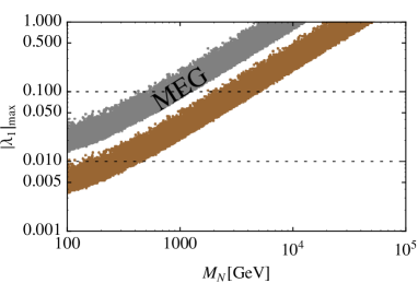
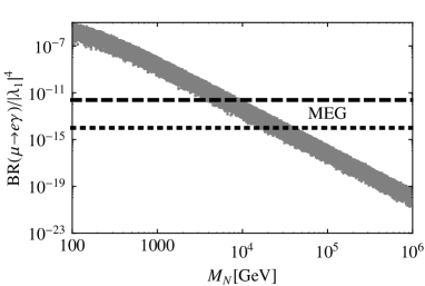
Figure 1: Decay branching ratio BR(μeγ)𝜇𝑒𝛾(\mu\to e\gamma) normalized to |𝛌𝟏|4superscriptsubscript𝛌14|\boldsymbol{\lambda_{1}}|^{4} for normal light neutrino mass spectrum as a function of the common RH neutrino mass (left hand side plot). The upper horizontal dashed line indicates the current limit on BR(μeγ)𝜇𝑒𝛾(\mu\to e\gamma) from the MEG experiment  [18], whereas the lower dotted one marks prospective future experimental sensitivities [19]. The corresponding bounds on |𝛌𝟏|subscript𝛌1|\boldsymbol{\lambda_{1}}| from the present [18] (upper gray band) and prospective future [19] (lower brown band) experimental searches are shown in the right hand side plot. The widths of the bands are due to the uncertainties in the neutrino mass matrix parameters. The results for the inverted neutrino spectrum are very similar and are thus not shown separately.

We find that radiative τ𝜏\tau decay rates are always below their current bounds and barely reach values of 109superscript10910^{-9} for RH neutrino masses around 100-200 GeV (values exceeding the current bounds are not consistent with the seesaw condition, that for concreteness we take as 𝒎𝑫𝑴𝑵1<101subscript𝒎𝑫superscriptsubscript𝑴𝑵1superscript101\boldsymbol{m_{D}}\boldsymbol{M_{N}}^{-1}<10^{-1}), we thus focus on the μeγ𝜇𝑒𝛾\mu\to e\gamma process. The results for the normal mass spectrum case are displayed in fig. 1 as a function of the common RH neutrino mass, MN=Msubscript𝑀𝑁𝑀M_{N}=M. We observe that BR(μeγ)𝜇𝑒𝛾(\mu\to e\gamma) can reach the current experimental limit reported by the MEG experiment [18] for RH neutrino masses MN<0.1TeV,1TeV,10subscript𝑀𝑁0.1TeV1TeV10M_{N}<0.1~{}\mathrm{TeV},1~{}\mathrm{TeV},~{}10 TeV provided |𝝀𝟏|2×102,101,1greater-than-or-equivalent-tosubscript𝝀12superscript102superscript1011|{\boldsymbol{\lambda_{1}}}|\gtrsim 2\times 10^{-2},~{}10^{-1},~{}1, respectively. The results for the inverted light neutrino mass hierarchy are very similar and consistent with these values. Finally we note that the widths of the bands in fig. 1 (and similarly for all the other considered processes below) are solely due to the uncertainties in the light neutrino mass matrix parameters (mainly θ13subscript𝜃13\theta_{13} and the CP violating phases) and can thus be improved with more precise light neutrino data.

3.2 liljljlj+superscriptsubscript𝑙𝑖superscriptsubscript𝑙𝑗superscriptsubscript𝑙𝑗superscriptsubscript𝑙𝑗l_{i}^{-}\to l_{j}^{-}l_{j}^{-}l_{j}^{+} processes

The decay branching ratios for these processes have been calculated in [21]. The most constrained process in this case is μe+eesuperscript𝜇superscript𝑒superscript𝑒superscript𝑒\mu^{-}\to e^{+}e^{-}e^{-} for which the SINDRUM experiment has placed a bound on the decay branching ratio of 1012superscript101210^{-12} at 90% C.L. [22]. For τe+eesuperscript𝜏superscript𝑒superscript𝑒superscript𝑒\tau^{-}\to e^{+}e^{-}e^{-} and τμ+μμsuperscript𝜏superscript𝜇superscript𝜇superscript𝜇\tau^{-}\to\mu^{+}\mu^{-}\mu^{-} the current bounds are 2.7×1082.7superscript1082.7\times 10^{-8} and 2.1×1082.1superscript1082.1\times 10^{-8}, respectively [23]. The decay branching ratios for these lepton flavor violating reactions are given by [21]

BR(lilj+ljlj+)BRsuperscriptsubscript𝑙𝑖superscriptsubscript𝑙𝑗superscriptsubscript𝑙𝑗superscriptsubscript𝑙𝑗\displaystyle\mbox{BR}(l_{i}^{-}\to l_{j}^{+}l_{j}^{-}l_{j}^{+}) =αW424576π3mi5MW41ΓTotalliabsentsuperscriptsubscript𝛼𝑊424576superscript𝜋3superscriptsubscript𝑚𝑖5superscriptsubscript𝑀𝑊41subscriptsuperscriptΓsubscript𝑙𝑖Total\displaystyle=\frac{\alpha_{W}^{4}}{24576\pi^{3}}\frac{m_{i}^{5}}{M_{W}^{4}}\frac{1}{\Gamma^{l_{i}}_{\text{Total}}}
{2|12FBoxli3lj+FZlilj2sW2(FZliljFγlilj)|2\displaystyle\left\{2\left|\frac{1}{2}F_{\text{Box}}^{l_{i}3l_{j}}+F_{Z}^{l_{i}l_{j}}-2s^{2}_{W}\left(F_{Z}^{l_{i}l_{j}}-F_{\gamma}^{l_{i}l_{j}}\right)\right|^{2}\right.
+4sW4|FZliljFγlilj|2+16sW2Re[(FZlilj+12FBoxli3lj)Gγlilj]4subscriptsuperscript𝑠4𝑊superscriptsuperscriptsubscript𝐹𝑍subscript𝑙𝑖subscript𝑙𝑗superscriptsubscript𝐹𝛾subscript𝑙𝑖subscript𝑙𝑗216subscriptsuperscript𝑠2𝑊Redelimited-[]superscriptsubscript𝐹𝑍subscript𝑙𝑖subscript𝑙𝑗12superscriptsubscript𝐹Boxsubscript𝑙𝑖3subscript𝑙𝑗superscriptsubscript𝐺𝛾subscript𝑙𝑖subscript𝑙𝑗\displaystyle\left.+4s^{4}_{W}\left|F_{Z}^{l_{i}l_{j}}-F_{\gamma}^{l_{i}l_{j}}\right|^{2}+16s^{2}_{W}\mbox{Re}\left[\left(F_{Z}^{l_{i}l_{j}}+\frac{1}{2}F_{\text{Box}}^{l_{i}3l_{j}}\right)G_{\gamma}^{l_{i}l_{j}*}\right]\right.
48sW4Re[(FZliljFγlilj)Gγlilj]+32sW4|Gγlilj|2(lnmi2mj2114)}.\displaystyle\left.-48s_{W}^{4}\mbox{Re}\left[\left(F_{Z}^{l_{i}l_{j}}-F_{\gamma}^{l_{i}l_{j}}\right)G_{\gamma}^{l_{i}l_{j}*}\right]+32s_{W}^{4}\left|G_{\gamma}^{l_{i}l_{j}}\right|^{2}\left(\ln\frac{m_{i}^{2}}{m_{j}^{2}}-\frac{11}{4}\right)\right\}\,. (22)

Here sW=sinθWsubscript𝑠𝑊subscript𝜃𝑊s_{W}=\sin\theta_{W}, where θWsubscript𝜃𝑊\theta_{W} is the weak mixing angle, and the functions Fγliljsuperscriptsubscript𝐹𝛾subscript𝑙𝑖subscript𝑙𝑗F_{\gamma}^{l_{i}l_{j}}, FZliljsuperscriptsubscript𝐹𝑍subscript𝑙𝑖subscript𝑙𝑗F_{Z}^{l_{i}l_{j}} and FBoxli3ljsubscriptsuperscript𝐹subscript𝑙𝑖3subscript𝑙𝑗BoxF^{l_{i}3l_{j}}_{\text{Box}} are form factors that involve the Yukawa couplings and loop functions arising from the γ𝛾\gamma, Z𝑍Z penguins and box diagrams that determine the the full process (see appendix A for a compilation of these expressions and ref. [21] for their derivation).

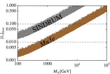
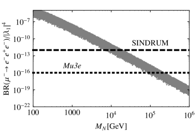
Following the same numerical procedure as in the liljγsubscript𝑙𝑖subscript𝑙𝑗𝛾l_{i}\to l_{j}\gamma case and using the form factors given in the appendix we evaluate the μ+e+eesuperscript𝜇superscript𝑒superscript𝑒superscript𝑒\mu^{+}\to e^{+}e^{-}e^{-}, τ+e+eesuperscript𝜏superscript𝑒superscript𝑒superscript𝑒\tau^{+}\to e^{+}e^{-}e^{-} and τ+μ+μμsuperscript𝜏superscript𝜇superscript𝜇superscript𝜇\tau^{+}\to\mu^{+}\mu^{-}\mu^{-} decay branching ratios for both, the normal and inverted light neutrino mass spectra. We find that τ+e+eesuperscript𝜏superscript𝑒superscript𝑒superscript𝑒\tau^{+}\to e^{+}e^{-}e^{-} and τ+μ+μμsuperscript𝜏superscript𝜇superscript𝜇superscript𝜇\tau^{+}\to\mu^{+}\mu^{-}\mu^{-} processes are always below 109similar-toabsentsuperscript109\sim 10^{-9} (due to the constraint enforced by the seesaw condition when |𝝀𝟏|>101subscript𝝀1superscript101|\boldsymbol{\lambda_{1}}|>10^{-1}), so in fig. 2 we only display the results for μ+e+eesuperscript𝜇superscript𝑒superscript𝑒superscript𝑒\mu^{+}\to e^{+}e^{-}e^{-}. We observe that the branching ratio can saturate the current experimental bound for RH neutrino masses MN<0.1TeV,1TeV,10subscript𝑀𝑁0.1TeV1TeV10M_{N}<0.1~{}\mathrm{TeV},1~{}\mathrm{TeV},~{}10 TeV provided |𝝀𝟏|2×102,101,1greater-than-or-equivalent-tosubscript𝝀12superscript102superscript1011|{\boldsymbol{\lambda_{1}}}|\gtrsim 2\times 10^{-2},~{}10^{-1},~{}1, respectively, very similar to the μeγ𝜇𝑒𝛾\mu\to e\gamma case. The results for the inverted light neutrino mass hierarchy are again very similar and consistent with these values. As can be seen by comparing figs. 1 and 2, with the sensitivities of the planned future experiments 555The proposed Mu3e experiment at PSI aims for a sensitivity of 1015superscript101510^{-15} in its first phase and 1016superscript101610^{-16} in its second phase [24]. this process has the potential to probe considerably larger values of the RH neutrino masses (compared with μeγ𝜇𝑒𝛾\mu\to e\gamma), reaching RH neutrino mass scales in excess of 𝒪(105GeV)𝒪superscript105GeV\mathcal{O}(10^{5}~{}{\rm GeV}) for |𝝀𝟏|1similar-tosubscript𝝀11|\boldsymbol{\lambda_{1}}|\sim 1. Finally we note that due to the strong |𝝀𝟏|subscript𝝀1|\boldsymbol{\lambda_{1}}| dependence, values of |𝝀𝟏|subscript𝝀1|\boldsymbol{\lambda_{1}}| below 103superscript10310^{-3} are not expected to yield observable rates at near future experimental facilities even for RH neutrino masses of the order 100 GeV.
Refer to caption
Refer to caption
Figure 2: Decay branching ratio BR(μee+e)\mu^{-}\to e^{-}e^{+}e^{-}) normalized to |𝛌𝟏|4superscriptsubscript𝛌14|\boldsymbol{\lambda_{1}}|^{4} for normal light neutrino mass spectrum as a function of common RH neutrino mass (left hand side plot). The upper horizontal dashed line indicates the current bound on the μe+eesuperscript𝜇superscript𝑒superscript𝑒superscript𝑒\mu^{-}\to e^{+}e^{-}e^{-} rate placed by the SINDRUM experiment  [22], whereas the lower dotted one illustrates prospective future experimental sensitivities of the Mu3e experiment [24]. The corresponding bounds on |𝛌𝟏|subscript𝛌1|\boldsymbol{\lambda_{1}}| from the present [22] (upper gray band) and prospective future [24] (lower brown band) experimental searches are shown in the right hand side plot. The widths of the bands are due to the uncertainties in the neutrino mass matrix parameters. The results for the inverted neutrino spectrum are very similar and are thus not shown separately.

3.3 μe𝜇𝑒\mu-e conversion in nuclei

Competitive lepton flavor violation constraints can also be obtained from searches for μe𝜇𝑒\mu-e conversion in nuclei. Currently the strongest bounds on BRμeΓconversion/Γcapture{}_{\mu e}\equiv\Gamma_{\text{conversion}}/\Gamma_{\text{capture}} were set by the SINDRUM collaboration from experiments on titanium with BR<μe(Ti)4.3×10¹²{}^{(\text{Ti})}_{\mu e}<4.3\times 10^{-12} [25] and gold target setting BR<μe(Au)7×10¹³{}_{\mu e}^{(\text{Au})}<7\times 10^{-13} [26], both at 90%CL. The μe𝜇𝑒\mu-e conversion bounds are expected to be further improved in the future by several orders of magnitude. According to proposals [27] and [28, 29], one can expect a sensitivity of 1016superscript101610^{-16} or even 1018superscript101810^{-18} by the PRISM/PRIME experiment.

To get the constraint in the μe𝜇𝑒\mu-e channel from these experiments, one needs to compute the relevant transition matrix elements in different nuclei. A detailed numerical calculation has been carried out by [30] and we use their formula in eq. (14) to calculate the desired conversion rates. They receive one-loop contributions from photonic penguins contributing to both effective dipole (ARsubscript𝐴𝑅A_{R}) and vector (gLV(u,d)subscriptsuperscript𝑔𝑢𝑑𝐿𝑉g^{(u,d)}_{LV}) couplings, as well as Z𝑍Z penguins and W𝑊W box diagrams (these only contribute to gLV(u,d)subscriptsuperscript𝑔𝑢𝑑𝐿𝑉g^{(u,d)}_{LV}). Using the notation of [30] we thus have

Γconversion=2GF2|ARD+(2gLV(u)+gLV(d))V(p)+(gLV(u)+2gLV(d))V(n)|2,subscriptΓconversion2superscriptsubscript𝐺𝐹2superscriptsuperscriptsubscript𝐴𝑅𝐷2superscriptsubscript𝑔𝐿𝑉𝑢superscriptsubscript𝑔𝐿𝑉𝑑superscript𝑉𝑝superscriptsubscript𝑔𝐿𝑉𝑢2superscriptsubscript𝑔𝐿𝑉𝑑superscript𝑉𝑛2\Gamma_{\text{conversion}}=2G_{F}^{2}\left|A_{R}^{*}D+(2g_{LV}^{(u)}+g_{LV}^{(d)})V^{(p)}+(g_{LV}^{(u)}+2g_{LV}^{(d)})V^{(n)}\right|^{2}\,, (23)

where GFsubscript𝐺𝐹G_{F} is the standard model Fermi coupling constant and ARsubscript𝐴𝑅A_{R}, gLV(u,d)superscriptsubscript𝑔𝐿𝑉𝑢𝑑g_{LV}^{(u,d)} are found to be (Qu,d=2/3,1/3subscript𝑄𝑢𝑑2313Q_{u,d}=2/3,-1/3):

ARsubscriptsuperscript𝐴𝑅\displaystyle A^{*}_{R} =28GFMW2αW8πGγμe,absent28subscript𝐺𝐹superscriptsubscript𝑀𝑊2subscript𝛼𝑊8𝜋subscriptsuperscript𝐺𝜇𝑒𝛾\displaystyle=\frac{\sqrt{2}}{8G_{F}M_{W}^{2}}\frac{\alpha_{W}}{8\pi}G^{\mu e}_{\gamma}\,, (24)
gLV(u)superscriptsubscript𝑔𝐿𝑉𝑢\displaystyle g_{LV}^{(u)} =2αW28GFMW2[(FZμe+4FBoxμ3e(1))4QusW2(FZμeFγμe)],absent2superscriptsubscript𝛼𝑊28subscript𝐺𝐹superscriptsubscript𝑀𝑊2delimited-[]superscriptsubscript𝐹𝑍𝜇𝑒4superscriptsubscript𝐹Box𝜇3𝑒14subscript𝑄𝑢superscriptsubscript𝑠𝑊2superscriptsubscript𝐹𝑍𝜇𝑒superscriptsubscript𝐹𝛾𝜇𝑒\displaystyle=\frac{\sqrt{2}\alpha_{W}^{2}}{8G_{F}M_{W}^{2}}\left[\left(F_{Z}^{\mu e}+4F_{\rm Box}^{\mu 3e(1)}\right)-4Q_{u}s_{W}^{2}\left(F_{Z}^{\mu e}-F_{\gamma}^{\mu e}\right)\right]\,, (25)
gLV(d)superscriptsubscript𝑔𝐿𝑉𝑑\displaystyle g_{LV}^{(d)} =2αW28GFMW2[(FZμe+FBoxμ3e(1))+4QdsW2(FZμeFγμe)].absent2superscriptsubscript𝛼𝑊28subscript𝐺𝐹superscriptsubscript𝑀𝑊2delimited-[]superscriptsubscript𝐹𝑍𝜇𝑒superscriptsubscript𝐹Box𝜇3𝑒14subscript𝑄𝑑superscriptsubscript𝑠𝑊2superscriptsubscript𝐹𝑍𝜇𝑒superscriptsubscript𝐹𝛾𝜇𝑒\displaystyle=-\frac{\sqrt{2}\alpha_{W}^{2}}{8G_{F}M_{W}^{2}}\left[\left(F_{Z}^{\mu e}+F_{\rm Box}^{\mu 3e(1)}\right)+4Q_{d}s_{W}^{2}\left(F_{Z}^{\mu e}-F_{\gamma}^{\mu e}\right)\right]\,. (26)
Nucleus D[mμ5/2]𝐷delimited-[]superscriptsubscript𝑚𝜇52D[m_{\mu}^{5/2}] V(p)[mμ5/2]superscript𝑉𝑝delimited-[]superscriptsubscript𝑚𝜇52V^{(p)}[m_{\mu}^{5/2}] V(n)[mμ5/2]superscript𝑉𝑛delimited-[]superscriptsubscript𝑚𝜇52V^{(n)}[m_{\mu}^{5/2}] Γcapture[106s1]subscriptΓcapturedelimited-[]superscript106superscript𝑠1\Gamma_{\text{capture}}[10^{6}s^{-1}]
Ti2248subscriptsuperscriptTi4822\text{\text{Ti}}^{48}_{22} 0.0864 0.0396 0.0468 2.59
Au79197subscriptsuperscriptAu19779\text{\text{Au}}^{197}_{79} 0.189 0.0974 0.146 13.07
Table 1: Data taken from Tables I and VIII of [30].

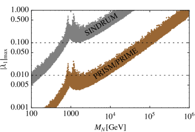
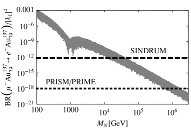
Following the same numerical procedure as in sections 3.1 and 3.2 we evaluate the resulting μe𝜇𝑒\mu-e conversion branching ratios. Since both Ti and Au processes feature the same flavor structure, the differences between them are entirely determined by the numerical factors quoted in table 1. The Ti parameters entering in the conversion rate are on average a factor 2.5similar-toabsent2.5\sim 2.5 smaller than the ones for Au, whereas the capture rates differ by a factor 5similar-toabsent5\sim 5. Accordingly the difference between these branching ratios is a factor of 2similar-toabsent2\sim 2. Due to its more stringent experimental upper bound we thus display only the results for Au in fig. 3 for the case of the normal light neutrino mass spectrum (the differences with the inverted mass spectrum case are again tiny). For MN1similar-tosubscript𝑀𝑁1M_{N}\sim 1 TeV the pieces proportional to V(p),(n)superscript𝑉𝑝𝑛V^{(p),(n)} in eq. (23) cancel, so the μe𝜇𝑒\mu-e conversion rate around this RH neutrino mass value is mainly controlled by the dipole contribution, ARDsuperscriptsubscript𝐴𝑅𝐷A_{R}^{*}D, which is roughly two orders of magnitude smaller. The dip in fig. 3 is due to this cancellation.

From fig. 3 it can be seen that the current experimental bound on this process imposes a constraint on the RH neutrino mass (as a function of |𝝀𝟏|subscript𝝀1|\boldsymbol{\lambda_{1}}|), which is roughly a factor of 2 stronger compared to bounds from μeγ𝜇𝑒𝛾\mu\to e\gamma and μ3e𝜇3𝑒\mu\to 3e (except for the region around MN1similar-tosubscript𝑀𝑁1M_{N}\sim 1 TeV, as explained above). Furthermore, given the expected future sensitivities, μAu79197eAu79197superscript𝜇superscriptsubscriptAu79197superscript𝑒superscriptsubscriptAu79197\mu^{-}\text{Au}_{79}^{197}\to e^{-}\text{Au}_{79}^{197} (and μTi2248eTi2248superscript𝜇superscriptsubscriptTi2248superscript𝑒superscriptsubscriptTi2248\mu^{-}\text{Ti}_{22}^{48}\to e^{-}\text{Ti}_{22}^{48}) could probe RH neutrino masses up to 𝒪(103TeV)𝒪superscript103TeV\mathcal{O}(10^{3}~{}\mathrm{TeV}) , far above the values accessible in μeγ𝜇𝑒𝛾\mu\to e\gamma and μee+esuperscript𝜇superscript𝑒superscript𝑒superscript𝑒\mu^{-}\to e^{-}e^{+}e^{-}, and thus constitutes the primary search channel for such scenarios of heavy RH neutrinos.
Refer to caption
Refer to caption
Figure 3: Branching ratio BR(μAu79197eAu79197superscript𝜇superscriptsubscriptAu79197superscript𝑒superscriptsubscriptAu79197\mu^{-}\mbox{\rm Au}_{79}^{197}\to e^{-}\mbox{\rm Au}_{79}^{197}) normalized to |𝛌𝟏|4superscriptsubscript𝛌14|\boldsymbol{\lambda_{1}}|^{4} as a function of the common RH neutrino mass for the light neutrino normal mass spectrum (left hand side plot). The upper horizontal dashed line indicates the current bound on this process settled by the SINDRUM experiment [26], whereas the lower one indicates future experimental sensitivities of the PRISM/PRIME experiment [27, 28, 29]. The corresponding bounds on |𝛌𝟏|subscript𝛌1|\boldsymbol{\lambda_{1}}| from the present [26] (upper gray band) and prospective future [27, 28, 29] (lower brown band) experimental searches are shown in the right hand side plot. The widths of the bands are due to the uncertainties in the neutrino mass matrix parameters. The results for the inverted neutrino spectrum are very similar and are thus not shown separately.

4 Primordial lepton asymmetries

We now turn to the issue of primordial lepton asymmetries and the related dynamics of the RH neutrinos. As we have discussed, different R𝑅R-charge assignments allow to define two types of models of which type B may yield sizable charged lepton flavor violating decays. For these effects to take place RH neutrino masses at or below the TeV scale as well as Yukawa couplings of order 102superscript10210^{-2} or larger are needed. The washouts induced by such couplings and in this mass range are so large that any lepton asymmetry generated via the out-of-equilibrium decays of the RH neutrinos will always yield a baryon asymmetry much smaller than the observed one [31]666In models with a slightly broken lepton number the washout is tiny, as it is determined by the amount of lepton number violation  [13]. In our case since lepton number is broken even in the U(1)R𝑈subscript1𝑅U(1)_{R} symmetric phase the washouts are dominated—as usual—by N1,2subscript𝑁12N_{1,2} inverse decays..

Either producing a baryon asymmetry consistent with the observed value or not erasing a preexisting one via the dynamics of the RH neutrino states (in case the RH neutrinos are still light and the resonant condition MN2MN1ΓN1similar-tosubscript𝑀subscript𝑁2subscript𝑀subscript𝑁1subscriptΓsubscript𝑁1M_{N_{2}}-M_{N_{1}}\sim\Gamma_{N_{1}} is not satisfied) requires small Yukawa couplings, thus rendering charged lepton flavor violating decay branching ratios negligibly small. The phenomenological requirements of sizable charged lepton flavor violating effects and the generation of a BL𝐵𝐿B-L asymmetry (or of not erasing a preexisting one) are therefore mutually exclusive. Since these requirements cover non-overlapped regions in parameter space they are from that point of view complementary.

The generation of a BL𝐵𝐿B-L asymmetry in the type B models discussed here follows quite closely the analysis done in ref. [32]. Thus, we do not discuss this issue here and instead study the constraints on parameter space derived from the condition of not erasing an assumed preexisting BL𝐵𝐿B-L asymmetry. Note that in type-I seesaw models with flavor symmetries in the lepton sector, as for example in MLFV models, the CP violating asymmetry in RH neutrino decays vanishes in the limit of exact flavor symmetry [33]. However, since in type B models the MLFV hypothesis is a consequence of the intrinsic structure of the model this does not happen.

In order to quantify these effects from now on we focus on the normal hierarchical light neutrino spectrum. Results for the inverted hierarchical case resemble quite closely the ones reported here. We start by recalling that the washouts induced by both RH neutrino states (at TMsimilar-to𝑇𝑀T\sim M) on any primordial BL𝐵𝐿B-L asymmetry are determined by the following set of kinetic equations:

dYΔidz=κi4j=e,μ,τCij()YΔjK1(z)z3.𝑑subscript𝑌subscriptΔ𝑖𝑑𝑧subscript𝜅𝑖4subscript𝑗𝑒𝜇𝜏subscriptsuperscript𝐶𝑖𝑗subscript𝑌subscriptΔ𝑗subscript𝐾1𝑧superscript𝑧3\frac{dY_{\Delta_{i}}}{dz}=-\frac{\kappa_{i}}{4}\sum_{j=e,\mu,\tau}C^{(\ell)}_{ij}\,Y_{\Delta_{j}}\,K_{1}(z)z^{3}\,. (27)

Here YX=(nXnX¯)/ssubscript𝑌𝑋subscript𝑛𝑋subscript𝑛¯𝑋𝑠Y_{X}=(n_{X}-n_{\bar{X}})/s (where nXsubscript𝑛𝑋n_{X} is the number density of particle X𝑋X and s𝑠s is the entropy density), z=M/T𝑧𝑀𝑇z=M/T and Δi=B/3LisubscriptΔ𝑖𝐵3subscript𝐿𝑖\Delta_{i}=B/3-L_{i} with Li=2i+eisubscript𝐿𝑖2subscript𝑖subscript𝑒𝑖L_{i}=2\ell_{i}+e_{i}. The function K1subscript𝐾1K_{1} is the modified Bessel function of the first type and the flavor coupling matrix 𝑪()superscript𝑪bold-ℓ\boldsymbol{C^{(\ell)}} is determined by the chemical equilibrium conditions imposed by the reactions that at the relevant temperature regime (TMsimilar-to𝑇𝑀T\sim M) are in thermal equilibrium [34]. The parameter κisubscript𝜅𝑖\kappa_{i}, that determines the strength of the flavored washouts, is given by

κi=m~imwherem~i=2v2M|λi1|2.formulae-sequencesubscript𝜅𝑖subscript~𝑚𝑖subscript𝑚wheresubscript~𝑚𝑖2superscript𝑣2𝑀superscriptsubscript𝜆𝑖12\kappa_{i}=\frac{\tilde{m}_{i}}{m_{\star}}\quad\mbox{where}\quad\tilde{m}_{i}=2\frac{v^{2}}{M}|\lambda_{i1}|^{2}\,. (28)

The factor m1.1×1012similar-to-or-equalssubscript𝑚1.1superscript1012m_{\star}\simeq 1.1\times 10^{-12} GeV. Note that in the basis in which the RH Majorana neutrino mass matrix is diagonal N1,2subscript𝑁12N_{1,2} couple to the lepton doublets with strength λi1subscript𝜆𝑖1\lambda_{i1}, the factor 2 in m~isubscript~𝑚𝑖\tilde{m}_{i} is due to this fact.

Refer to caption
Refer to caption
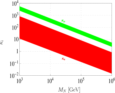
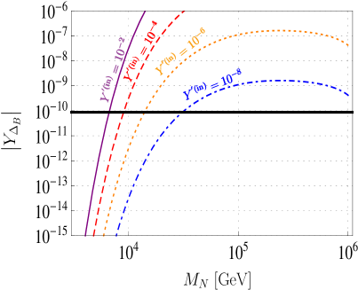
Figure 4: Left hand side plot: washout factors for muon and electron lepton flavors as a function of the common RH neutrino mass in the case of a normal hierarchical spectrum. Right hand side plot: |YΔB|subscript𝑌subscriptΔ𝐵|Y_{\Delta_{B}}| as a function of the common RH neutrino mass for several values of the assumed primordial BL𝐵𝐿B-L asymmetry. The solid (black) horizontal line indicates the observed value of the baryon asymmetry. See the text for more details.

According to the parametrization in eq. (13) the κisubscript𝜅𝑖\kappa_{i} parameters can be written as

κi=v2m|𝝀𝟏|2M|λ^i1|2=v2m|𝝀𝟏|2M|1+ρUi3+1ρUi2|2.subscript𝜅𝑖superscript𝑣2subscript𝑚superscriptsubscript𝝀12𝑀superscriptsubscript^𝜆𝑖12superscript𝑣2subscript𝑚superscriptsubscript𝝀12𝑀superscript1𝜌superscriptsubscript𝑈𝑖31𝜌superscriptsubscript𝑈𝑖22\displaystyle\kappa_{i}=\frac{v^{2}}{m_{\star}}\,\frac{|\boldsymbol{\lambda_{1}}|^{2}}{M}|\hat{\lambda}_{i1}|^{2}=\frac{v^{2}}{m_{\star}}\,\frac{|\boldsymbol{\lambda_{1}}|^{2}}{M}\left|\sqrt{1+\rho}\,U_{i3}^{*}+\sqrt{1-\rho}\,U_{i2}^{*}\right|^{2}\,. (29)

Thus, after fixing low-energy observables the values of the parameters κisubscript𝜅𝑖\kappa_{i} depend only on M𝑀M and |𝝀𝟏|subscript𝝀1|\boldsymbol{\lambda_{1}}|. Fig. 4 (left hand side plot) shows an example for the values of κe,μsubscript𝜅𝑒𝜇\kappa_{e,\mu} (the κτsubscript𝜅𝜏\kappa_{\tau} is smaller than κμsubscript𝜅𝜇\kappa_{\mu} by less than a factor 10) obtained by enforcing neutrino data to lie within their 2σ2𝜎2\sigma experimental ranges [1] and fixing for concreteness |𝝀𝟏|=105subscript𝝀1superscript105|\boldsymbol{\lambda_{1}}|=10^{-5}. As can be seen, if the preexisting asymmetry is sufficiently large even in the case of light RH neutrinos a sizable asymmetry in the electron flavor could be stored.

An estimation of the N1,2subscript𝑁12N_{1,2} washout effects can be easily done in the one-flavor approximation by taking 𝑪()=𝕀superscript𝑪bold-ℓ𝕀\boldsymbol{C^{(\ell)}}=\boldsymbol{\mathds{I}} in eq. (27). The resulting equation can be analytically integrated yielding the following result for the final baryon asymmetry:

YΔB=1237YΔBL(in)e3πκ/8.subscript𝑌subscriptΔ𝐵1237superscriptsubscript𝑌subscriptΔ𝐵𝐿insuperscript𝑒3𝜋𝜅8Y_{\Delta_{B}}=\frac{12}{37}\,Y_{\Delta_{B-L}}^{(\text{in})}\,e^{-3\pi\kappa/8}\,. (30)

From this equation a parametric relation between the relevant parameters can be calculated, namely

|𝝀𝟏|2M=8m3πv2log(1237YΔBL(in)YΔB),superscriptsubscript𝝀12𝑀8subscript𝑚3𝜋superscript𝑣21237superscriptsubscript𝑌subscriptΔ𝐵𝐿insubscript𝑌subscriptΔ𝐵\frac{|\boldsymbol{\lambda_{1}}|^{2}}{M}=\frac{8m_{\star}}{3\pi v^{2}}\log\left(\frac{12}{37}\frac{Y_{\Delta_{B-L}}^{(\text{in})}}{Y_{\Delta_{B}}}\right)\,, (31)

thus fixing YΔBsubscript𝑌subscriptΔ𝐵Y_{\Delta_{B}} to its central value (YΔB=8.75×10¹¹subscript𝑌subscriptΔ𝐵8.75superscript1011Y_{\Delta_{B}}=8.75\times 10^{-11} [31]) and taking YΔBL(in)[108,102]superscriptsubscript𝑌subscriptΔ𝐵𝐿insuperscript108superscript102Y_{\Delta_{B-L}}^{(\text{in})}\subset[10^{-8},10^{-2}] it turns out that as long as |𝝀𝟏|2/M[1,5]×1016GeV1superscriptsubscript𝝀12𝑀15superscript1016superscriptGeV1|\boldsymbol{\lambda_{1}}|^{2}/M\subset[1,5]\times 10^{-16}\;\mbox{GeV}^{-1} a primordial asymmetry may always survive the N1,2subscript𝑁12N_{1,2} related washouts and yield a value consistent with the observed one.

A precise treatment, however, requires the inclusion of flavor. In the mass range we are interested in ([103,106]superscript103superscript106[10^{3},10^{6}] GeV) all the standard model Yukawa processes (quarks and leptons) are in thermodynamical equilibrium [34]. Neglecting order one spectator processes, the kinetic eqs. (27) consist of three coupled differential equations accounting for the evolution of the Δτ,μ,esubscriptΔ𝜏𝜇𝑒\Delta_{\tau,\mu,e} asymmetries. Defining the asymmetry vector 𝒀𝚫=(YΔτ,YΔμ,YΔe)subscript𝒀𝚫subscript𝑌subscriptΔ𝜏subscript𝑌subscriptΔ𝜇subscript𝑌subscriptΔ𝑒\boldsymbol{Y_{\Delta}}=(Y_{\Delta_{\tau}},Y_{\Delta_{\mu}},Y_{\Delta_{e}}) the system of coupled equations can be arranged in a single equation

ddz𝒀𝚫=v24m|𝝀𝟏|2M𝑪~()𝒀𝚫K1(z)z3,𝑑𝑑𝑧subscript𝒀𝚫superscript𝑣24subscript𝑚superscriptsubscript𝝀12𝑀superscriptbold-~𝑪bold-ℓsubscript𝒀𝚫subscript𝐾1𝑧superscript𝑧3\frac{d}{dz}\boldsymbol{Y_{\Delta}}=-\frac{v^{2}}{4m_{\star}}\frac{|\boldsymbol{\lambda_{1}}|^{2}}{M}\,\boldsymbol{\tilde{C}^{(\ell)}}\;\boldsymbol{Y_{\Delta}}K_{1}(z)z^{3}\,, (32)

where C~ij()=|λ^i1|2Cij()subscriptsuperscript~𝐶𝑖𝑗superscriptsubscript^𝜆𝑖12subscriptsuperscript𝐶𝑖𝑗\tilde{C}^{(\ell)}_{ij}=|\hat{\lambda}_{i1}|^{2}C^{(\ell)}_{ij} and the matrix 𝑪()superscript𝑪bold-ℓ\boldsymbol{C^{(\ell)}}, at this stage, is given by [34]

𝑪()=1711(221161616221161616221).superscript𝑪bold-ℓ1711matrix221161616221161616221\boldsymbol{C^{(\ell)}}=\frac{1}{711}\begin{pmatrix}221&-16&-16\\ -16&221&-16\\ -16&-16&221\end{pmatrix}\,. (33)

By rotating the asymmetry vector in the direction in which 𝑪~()superscriptbold-~𝑪bold-ℓ\boldsymbol{\tilde{C}^{(\ell)}} becomes diagonal (𝒀𝚫=𝑷𝒀𝚫superscriptsubscript𝒀𝚫𝑷subscript𝒀𝚫\boldsymbol{Y_{\Delta}}^{\prime}=\boldsymbol{P}\,\boldsymbol{Y_{\Delta}}) the system of equations can be decoupled and thus solved analytically for 𝒀𝚫superscriptsubscript𝒀𝚫\boldsymbol{Y_{\Delta}}^{\prime} as in the unflavored regime:

ddz𝒀𝚫=v24m|𝝀𝟏|2M𝑪~diag()𝒀𝚫K1(z)z3with𝑷𝑪~()𝑷𝟏=𝑪~diag().formulae-sequence𝑑𝑑𝑧superscriptsubscript𝒀𝚫superscript𝑣24subscript𝑚superscriptsubscript𝝀12𝑀subscriptsuperscriptbold-~𝑪bold-ℓdiagsuperscriptsubscript𝒀𝚫subscript𝐾1𝑧superscript𝑧3with𝑷superscriptbold-~𝑪bold-ℓsuperscript𝑷1subscriptsuperscriptbold-~𝑪bold-ℓdiag\frac{d}{dz}\boldsymbol{Y_{\Delta}}^{\prime}=-\frac{v^{2}}{4m_{\star}}\frac{|\boldsymbol{\lambda_{1}}|^{2}}{M}\,\boldsymbol{\tilde{C}^{(\ell)}_{\text{diag}}}\;\boldsymbol{Y_{\Delta}}^{\prime}K_{1}(z)z^{3}\quad\mbox{with}\quad\boldsymbol{P}\boldsymbol{\tilde{C}^{(\ell)}}\boldsymbol{P^{-1}}=\boldsymbol{\tilde{C}^{(\ell)}_{\text{diag}}}\,. (34)

The solution reads

YΔi=YΔi(in)e3πκc~i/8,Y_{\Delta_{i}}^{\prime}=Y_{\Delta_{i}}^{{}^{\prime}(\text{in})}\,e^{-3\pi\kappa\tilde{c}_{i}/8}\,, (35)

where the c~isubscript~𝑐𝑖\tilde{c}_{i}’s (i=τ,μ,e𝑖𝜏𝜇𝑒i=\tau,\mu,e) are the eigenvalues of the matrix 𝑪~()superscriptbold-~𝑪bold-ℓ\boldsymbol{\tilde{C}^{(\ell)}}. The final baryon asymmetry in this case is therefore given by

YΔB=1237j=τ,μ,eYΔj=1237j,i=τ,μ,e(𝑷1)jiYΔi(in)e3πκc~i/8.Y_{\Delta_{B}}=\frac{12}{37}\sum_{j=\tau,\mu,e}Y_{\Delta_{j}}=\frac{12}{37}\sum_{j,i=\tau,\mu,e}\left(\boldsymbol{P}^{-1}\right)_{ji}Y_{\Delta_{i}}^{{}^{\prime}(\text{in})}\,e^{-3\pi\kappa\tilde{c}_{i}/8}\,. (36)

In order to illustrate the effects of the N1,2subscript𝑁12N_{1,2} related washouts on a preexisting BL𝐵𝐿B-L asymmetry we fix the light neutrino mixing angles and the atmospheric and solar scales to their best fit point values [1], δ=π/2𝛿𝜋2\delta=\pi/2, ϕ=0italic-ϕ0\phi=0 and again |𝝀𝟏|=105subscript𝝀1superscript105|\boldsymbol{\lambda_{1}}|=10^{-5}. Assuming the same primordial ΔisubscriptΔ𝑖\Delta_{i} asymmetries in each flavor, varying them from 108102superscript108superscript10210^{-8}-10^{-2}, and using eq.  (36) we calculate the resulting YΔBsubscript𝑌subscriptΔ𝐵Y_{\Delta_{B}} asymmetry. The results are displayed in fig. 4 (right hand side plot). It can be seen that for the set of parameters chosen a YΔBsubscript𝑌subscriptΔ𝐵Y_{\Delta_{B}} in the observed range can always be obtained.

5 Conclusions

Besides the global total lepton number U(1)L𝑈subscript1𝐿U(1)_{L} the canonical seesaw mechanism also breaks a global U(1)R𝑈subscript1𝑅U(1)_{R} symmetry respected by the kinetic and gauge terms in the SM Lagrangian. In the context of MLFV models, this U(1)R𝑈subscript1𝑅U(1)_{R} can be identified with global phase rotations of the charged lepton electroweak singlets e𝑒e or RH neutrinos N𝑁N. In this paper we have explored the implications of a slightly broken U(1)R𝑈subscript1𝑅U(1)_{R} symmetry in the context of minimal seesaw setups (with two RH neutrinos). We have shown that depending on the R𝑅R-charge assignments two classes of generic models can be identified: (type A𝐴A) models where the small breaking of U(1)R𝑈subscript1𝑅U(1)_{R} allows to decouple the lepton number breaking scale from the RH neutrino mass scale [8]; (type B𝐵B) models where the parameters that slightly break the U(1)R𝑈subscript1𝑅U(1)_{R} induce a suppression in the light neutrino mass matrix.

We have studied the implications of these models for charged lepton flavor violating decays. We found that in type A models the decoupling of the RH neutrino masses from the lepton number breaking scale implies also a suppression of the corresponding Yukawa couplings, thus leading to non-observable charged lepton flavor violating effects. Type B models realize the MLFV hypothesis in the sense that due to the structure of the light neutrino mass matrix their flavor patterns are—up to normalization factors—entirely determined by low-energy neutrino observables. Moreover, the suppression induced by the slightly broken U(1)R𝑈subscript1𝑅U(1)_{R} on the neutrino mass matrix allows large Yukawa couplings and TeV RH neutrino masses, and thus potentially large flavor violating μ𝜇\mu processes. We have studied the μeγ𝜇𝑒𝛾\mu\to e\gamma, μ3e𝜇3𝑒\mu\to 3e and μe𝜇𝑒\mu-e conversion in nuclei for normal and inverted neutrino mass spectra, finding that the three processes have branching ratios accessible in present experiments as long as the relevant overall Yukawa normalization factor is larger than 102,101,1similar-toabsentsuperscript102superscript1011\sim 10^{-2},10^{-1},1 and the RH neutrino masses are below 0.1TeV,1TeV,10similar-toabsent0.1TeV1TeV10\sim 0.1~{}\mathrm{TeV},1~{}\mathrm{TeV},10~{}TeV, respectively. For heavier RH neutrinos μeγ𝜇𝑒𝛾\mu\to e\gamma is below prospective future sensitivities while μ3e𝜇3𝑒\mu\to 3e and μe𝜇𝑒\mu-e conversion in nuclei would remain observable, up to MN100similar-tosubscript𝑀𝑁100M_{N}\sim 100 TeV and MN103similar-tosubscript𝑀𝑁superscript103M_{N}\sim 10^{3} TeV respectively. On the other hand in both type A and B models, RH neutrino contributions to LFV tau lepton decays are restricted below the present and near future experimental sensitivities.

Sizable μ𝜇\mu flavor violating decays require large Yukawa couplings and light RH neutrinos. These values imply large RH neutrino inverse decay effects, that render the dynamics of these states incompatible with either the generation of a BL𝐵𝐿B-L asymmetry (consistent with the observed B𝐵B asymmetry) or with the preservation of a preexisting one. Accordingly, sizable lepton flavor processes and small RH neutrino inverse decay effects are phenomenological requirements that cover non-overlapping regions of parameter space, from that point of view the analysis of both of them turns out to be complementary. In the low mass range (M106less-than-or-similar-to𝑀superscript106M\lesssim 10^{6} GeV), instead of studying the generation of a BL𝐵𝐿B-L asymmetry via resonant leptogenesis, we have considered the influence of the RH neutrino dynamics on a primordial BL𝐵𝐿B-L asymmetry. We have demonstrated that a preexisting asymmetry yielding the observed B𝐵B asymmetry can survive the RH neutrino related washouts provided the overall Yukawa coupling normalization is below 105similar-toabsentsuperscript105\sim 10^{-5} .

Acknowledgments

We want to thank G. Isidori and E. Nardi and M. Hirsch for useful comments and remarks. DAS is supported by a belgian FNRS fellowship. The work of JFK was supported in part by the Slovenian Research Agency. DAS and AD want to thank the Josef Stefan Institute for the kind hospitality during the completion of this work.

Appendix A Formulas for liljγsubscript𝑙𝑖subscript𝑙𝑗𝛾l_{i}\to l_{j}\gamma and liljlj+ljsuperscriptsubscript𝑙𝑖superscriptsubscript𝑙𝑗superscriptsubscript𝑙𝑗superscriptsubscript𝑙𝑗l_{i}^{-}\to l_{j}^{-}l_{j}^{+}l_{j}^{-} processes

In this appendix we summarize the formulas we use for the calculation of the charged lepton flavor violating decays discussed in sections 3.1 and 3.2. The results presented here were extracted from ref. [21] and adapted to our notation. In what follows the parameters rasubscript𝑟𝑎r_{a}’s are defined according to ra=MW2/MNa2subscript𝑟𝑎superscriptsubscript𝑀𝑊2superscriptsubscript𝑀subscript𝑁𝑎2r_{a}=M_{W}^{2}/M_{N_{a}}^{2}.

The process liljlj+ljsuperscriptsubscript𝑙𝑖superscriptsubscript𝑙𝑗superscriptsubscript𝑙𝑗superscriptsubscript𝑙𝑗l_{i}^{-}\to l_{j}^{-}l_{j}^{+}l_{j}^{-} is determined by γ𝛾\gamma, and Z𝑍Z penguins and box diagrams (for the full set of Feynman diagrams see ref. [21]). The γ𝛾\gamma penguin contribution can be split in two pieces corresponding to the photon being either on-shell or off-shell. For the on-shell piece, the one that determines the liljγsubscript𝑙𝑖subscript𝑙𝑗𝛾l_{i}\to l_{j}\gamma process, we have

Gγliljsuperscriptsubscript𝐺𝛾subscript𝑙𝑖subscript𝑙𝑗\displaystyle G_{\gamma}^{l_{i}l_{j}} =2g2(𝝀𝑮𝜸𝝀)ij,absent2superscript𝑔2subscript𝝀subscript𝑮𝜸superscript𝝀𝑖𝑗\displaystyle=\frac{2}{g^{2}}\left(\boldsymbol{\lambda}\cdot\boldsymbol{G_{\gamma}}\cdot\boldsymbol{\lambda}^{\dagger}\right)_{ij}\,, (37)
Gγ(ra)subscript𝐺𝛾subscript𝑟𝑎\displaystyle G_{\gamma}(r_{a}) =ra4(1ra)4(2+3ra6ra2+ra3+6ralogra),absentsubscript𝑟𝑎4superscript1subscript𝑟𝑎423subscript𝑟𝑎6superscriptsubscript𝑟𝑎2superscriptsubscript𝑟𝑎36subscript𝑟𝑎subscript𝑟𝑎\displaystyle=\frac{r_{a}}{4(1-r_{a})^{4}}\left(2+3r_{a}-6r_{a}^{2}+r_{a}^{3}+6r_{a}\log r_{a}\right)\,, (38)

whereas for the off-shell photon piece

Fγliljsuperscriptsubscript𝐹𝛾subscript𝑙𝑖subscript𝑙𝑗\displaystyle F_{\gamma}^{l_{i}l_{j}} =2g2(𝝀𝑭𝜸𝝀)ij,absent2superscript𝑔2subscript𝝀subscript𝑭𝜸superscript𝝀𝑖𝑗\displaystyle=\frac{2}{g^{2}}\left(\boldsymbol{\lambda}\cdot\boldsymbol{F_{\gamma}}\cdot\boldsymbol{\lambda}^{\dagger}\right)_{ij}\,, (39)
Fγ(ra)subscript𝐹𝛾subscript𝑟𝑎\displaystyle F_{\gamma}(r_{a}) =ra12(1ra)4[78ra11ra2+12ra3(220ra+24ra2)logra].absentsubscript𝑟𝑎12superscript1subscript𝑟𝑎4delimited-[]78subscript𝑟𝑎11superscriptsubscript𝑟𝑎212superscriptsubscript𝑟𝑎3220subscript𝑟𝑎24superscriptsubscript𝑟𝑎2subscript𝑟𝑎\displaystyle=-\frac{r_{a}}{12(1-r_{a})^{4}}\left[7-8r_{a}-11r_{a}^{2}+12r_{a}^{3}-(2-20r_{a}+24r_{a}^{2})\log r_{a}\right]\,. (40)

The Z𝑍Z penguin contribution can be split in two parts, namely

FZlilj=FZlilj(1)+FZlilj(2),superscriptsubscript𝐹𝑍subscript𝑙𝑖subscript𝑙𝑗superscriptsubscript𝐹𝑍subscript𝑙𝑖subscript𝑙𝑗1superscriptsubscript𝐹𝑍subscript𝑙𝑖subscript𝑙𝑗2F_{Z}^{l_{i}l_{j}}=F_{Z}^{l_{i}l_{j}(1)}+F_{Z}^{l_{i}l_{j}(2)}\,, (41)

where the first piece can be written as

FZlilj(1)superscriptsubscript𝐹𝑍subscript𝑙𝑖subscript𝑙𝑗1\displaystyle F_{Z}^{l_{i}l_{j}(1)} =2g2[𝝀(𝑭^𝒁+𝑮^𝒁(𝟏))𝝀]ij,absent2superscript𝑔2subscriptdelimited-[]𝝀subscriptbold-^𝑭𝒁superscriptsubscriptbold-^𝑮𝒁1superscript𝝀𝑖𝑗\displaystyle=\frac{2}{g^{2}}\left[\boldsymbol{\lambda}\cdot\left(\boldsymbol{\hat{F}_{Z}}+\boldsymbol{\hat{G}_{Z}^{(1)}}\right)\cdot\boldsymbol{\lambda}^{\dagger}\right]_{ij}\,, (42)
FZ(ra)subscript𝐹𝑍subscript𝑟𝑎\displaystyle F_{Z}(r_{a}) =5ra2(1ra)2(1ra+logra),absent5subscript𝑟𝑎2superscript1subscript𝑟𝑎21subscript𝑟𝑎subscript𝑟𝑎\displaystyle=\frac{5r_{a}}{2(1-r_{a})^{2}}\left(1-r_{a}+\log r_{a}\right)\,, (43)
GZ(1)(ra)superscriptsubscript𝐺𝑍1subscript𝑟𝑎\displaystyle G_{Z}^{(1)}(r_{a}) =ra1ralogra,absentsubscript𝑟𝑎1subscript𝑟𝑎subscript𝑟𝑎\displaystyle=-\frac{r_{a}}{1-r_{a}}\log r_{a}\,, (44)

while the second contribution according to

FZlilj(2)superscriptsubscript𝐹𝑍subscript𝑙𝑖subscript𝑙𝑗2\displaystyle F_{Z}^{l_{i}l_{j}(2)} =4g4[𝝀(𝑮~𝒁(𝟐)+𝑮~𝒁(𝟑)+𝑮~𝒁(𝟒)+𝑯~𝒁)𝝀]ij,absent4superscript𝑔4subscriptdelimited-[]𝝀superscriptsubscriptbold-~𝑮𝒁2superscriptsubscriptbold-~𝑮𝒁3superscriptsubscriptbold-~𝑮𝒁4subscriptbold-~𝑯𝒁superscript𝝀𝑖𝑗\displaystyle=\frac{4}{g^{4}}\left[\boldsymbol{\lambda}\cdot\left(\boldsymbol{\tilde{G}_{Z}^{(2)}}+\boldsymbol{\tilde{G}_{Z}^{(3)}}+\boldsymbol{\tilde{G}_{Z}^{(4)}}+\boldsymbol{\tilde{H}_{Z}}\right)\cdot\boldsymbol{\lambda}^{\dagger}\right]_{ij}\,, (45)
G~Z(A)(ra,rb)superscriptsubscript~𝐺𝑍𝐴subscript𝑟𝑎subscript𝑟𝑏\displaystyle\tilde{G}_{Z}^{(A)}(r_{a},r_{b}) =(𝝀𝝀)abGZ(A)(ra,rb)withA=2,3,4,formulae-sequenceabsentsubscriptsuperscript𝝀𝝀𝑎𝑏superscriptsubscript𝐺𝑍𝐴subscript𝑟𝑎subscript𝑟𝑏with𝐴234\displaystyle=(\boldsymbol{\lambda}^{\dagger}\cdot\boldsymbol{\lambda})_{ab}G_{Z}^{(A)}(r_{a},r_{b})\quad\mbox{with}\quad A=2,3,4\,, (46)
GZ(2)(ra,rb)superscriptsubscript𝐺𝑍2subscript𝑟𝑎subscript𝑟𝑏\displaystyle G_{Z}^{(2)}(r_{a},r_{b}) =rarb2(rarb)(1rb1ralogra1ra1rblogrb),absentsubscript𝑟𝑎subscript𝑟𝑏2subscript𝑟𝑎subscript𝑟𝑏1subscript𝑟𝑏1subscript𝑟𝑎subscript𝑟𝑎1subscript𝑟𝑎1subscript𝑟𝑏subscript𝑟𝑏\displaystyle=-\frac{r_{a}r_{b}}{2(r_{a}-r_{b})}\left(\frac{1-r_{b}}{1-r_{a}}\log r_{a}-\frac{1-r_{a}}{1-r_{b}}\log r_{b}\right)\,, (47)
GZ(3)(ra,rb)superscriptsubscript𝐺𝑍3subscript𝑟𝑎subscript𝑟𝑏\displaystyle G_{Z}^{(3)}(r_{a},r_{b}) =rarb2(1ra)logra,absentsubscript𝑟𝑎subscript𝑟𝑏21subscript𝑟𝑎subscript𝑟𝑎\displaystyle=\frac{r_{a}r_{b}}{2(1-r_{a})}\log r_{a}\,, (48)
GZ(4)(ra,rb)superscriptsubscript𝐺𝑍4subscript𝑟𝑎subscript𝑟𝑏\displaystyle G_{Z}^{(4)}(r_{a},r_{b}) =rarb2(1rb)logrb,absentsubscript𝑟𝑎subscript𝑟𝑏21subscript𝑟𝑏subscript𝑟𝑏\displaystyle=\frac{r_{a}r_{b}}{2(1-r_{b})}\log r_{b}\,, (49)
H~Z(ra,rb)subscript~𝐻𝑍subscript𝑟𝑎subscript𝑟𝑏\displaystyle\tilde{H}_{Z}(r_{a},r_{b}) =(𝝀T𝝀)abHZ(ra,rb),absentsubscriptsuperscript𝝀𝑇superscript𝝀𝑎𝑏subscript𝐻𝑍subscript𝑟𝑎subscript𝑟𝑏\displaystyle=\left(\boldsymbol{\lambda}^{T}\cdot\boldsymbol{\lambda}^{*}\right)_{ab}H_{Z}(r_{a},r_{b})\,, (50)
HZ(ra,rb)subscript𝐻𝑍subscript𝑟𝑎subscript𝑟𝑏\displaystyle H_{Z}(r_{a},r_{b}) =rarb4(rarb)[rb(14ra)1ralograra(14rb)1rblogrb].absentsubscript𝑟𝑎subscript𝑟𝑏4subscript𝑟𝑎subscript𝑟𝑏delimited-[]subscript𝑟𝑏14subscript𝑟𝑎1subscript𝑟𝑎subscript𝑟𝑎subscript𝑟𝑎14subscript𝑟𝑏1subscript𝑟𝑏subscript𝑟𝑏\displaystyle=-\frac{\sqrt{r_{a}r_{b}}}{4(r_{a}-r_{b})}\left[\frac{r_{b}(1-4r_{a})}{1-r_{a}}\log r_{a}-\frac{r_{a}(1-4r_{b})}{1-r_{b}}\log r_{b}\right]\,. (51)

Note that due to the constraint implied by the SU(3)+N𝑆𝑈subscript3𝑁SU(3)_{\ell+N} flavor symmetry the off-diagonal elements of the matrices G~Z(A)(ra,rb)superscriptsubscript~𝐺𝑍𝐴subscript𝑟𝑎subscript𝑟𝑏\tilde{G}_{Z}^{(A)}(r_{a},r_{b}) and H~Z(A)(ra,rb)superscriptsubscript~𝐻𝑍𝐴subscript𝑟𝑎subscript𝑟𝑏\tilde{H}_{Z}^{(A)}(r_{a},r_{b}) vanish.

The box diagram contributions can be split in three parts as follows

FBoxli3lj=A=1,2,3FBoxli3lj(A),subscriptsuperscript𝐹subscript𝑙𝑖3subscript𝑙𝑗Boxsubscript𝐴123subscriptsuperscript𝐹subscript𝑙𝑖3subscript𝑙𝑗𝐴BoxF^{l_{i}3l_{j}}_{\text{Box}}=\sum_{A=1,2,3}F^{l_{i}3l_{j}(A)}_{\text{Box}}\,, (52)

For the first part we have

FBoxli3lj(1)subscriptsuperscript𝐹subscript𝑙𝑖3subscript𝑙𝑗1Box\displaystyle F^{l_{i}3l_{j}(1)}_{\text{Box}} =2g2[𝝀𝑭^Box(𝟏)𝝀]ij,absent2superscript𝑔2subscriptdelimited-[]𝝀superscriptsubscriptbold-^𝑭Box1superscript𝝀𝑖𝑗\displaystyle=\frac{2}{g^{2}}\left[\boldsymbol{\lambda}\cdot\boldsymbol{\hat{F}_{\text{Box}}^{(1)}}\cdot\boldsymbol{\lambda}^{\dagger}\right]_{ij}\,, (53)
FBox(1)(ra)superscriptsubscript𝐹Box1subscript𝑟𝑎\displaystyle F_{\text{Box}}^{(1)}(r_{a}) =2ra(1ra)2(1ra+ralogra).absent2subscript𝑟𝑎superscript1subscript𝑟𝑎21subscript𝑟𝑎subscript𝑟𝑎subscript𝑟𝑎\displaystyle=-\frac{2r_{a}}{(1-r_{a})^{2}}\left(1-r_{a}+r_{a}\log r_{a}\right)\,. (54)

For the second is given by

FBoxli3lj(2)(j)subscriptsuperscript𝐹subscript𝑙𝑖3subscript𝑙𝑗2Box𝑗\displaystyle F^{l_{i}3l_{j}(2)}_{\text{Box}}(j) =4g4[𝝀(𝑭~Box(𝟐)(j)+𝑭~Box(𝟑)(j))𝝀]ij,absent4superscript𝑔4subscriptdelimited-[]𝝀superscriptsubscriptbold-~𝑭Box2𝑗superscriptsubscriptbold-~𝑭Box3𝑗superscript𝝀𝑖𝑗\displaystyle=\frac{4}{g^{4}}\left[\boldsymbol{\lambda}\cdot\left(\boldsymbol{\tilde{F}_{\text{Box}}^{(2)}}(j)+\boldsymbol{\tilde{F}_{\text{Box}}^{(3)}}(j)\right)\cdot\boldsymbol{\lambda}^{\dagger}\right]_{ij}\,, (55)
F~Box(A)(ra,rb)(j)superscriptsubscript~𝐹Box𝐴subscript𝑟𝑎subscript𝑟𝑏𝑗\displaystyle\tilde{F}_{\text{Box}}^{(A)}(r_{a},r_{b})(j) =λjaFBox(A)(ra,rb)λjbwithA=2,3,formulae-sequenceabsentsubscriptsuperscript𝜆𝑗𝑎superscriptsubscript𝐹Box𝐴subscript𝑟𝑎subscript𝑟𝑏subscript𝜆𝑗𝑏with𝐴23\displaystyle=\lambda^{*}_{ja}\;F_{\text{Box}}^{(A)}(r_{a},r_{b})\;\lambda_{jb}\quad\mbox{with}\quad A=2,3\,, (56)
FBox(2)(ra,rb)superscriptsubscript𝐹Box2subscript𝑟𝑎subscript𝑟𝑏\displaystyle F_{\text{Box}}^{(2)}(r_{a},r_{b}) =rarb4(rarb)[14ra(2rb)(1ra)2logra14rb(2ra)(1rb)2logrb\displaystyle=\frac{r_{a}r_{b}}{4(r_{a}-r_{b})}\left[\frac{1-4r_{a}(2-r_{b})}{(1-r_{a})^{2}}\log r_{a}-\frac{1-4r_{b}(2-r_{a})}{(1-r_{b})^{2}}\log r_{b}\right.
rarb(1ra)(1rb)(74rarb)],\displaystyle\left.-\frac{r_{a}-r_{b}}{(1-r_{a})(1-r_{b})}(7-4r_{a}r_{b})\right]\,, (57)
FBox(3)(ra,rb)superscriptsubscript𝐹Box3subscript𝑟𝑎subscript𝑟𝑏\displaystyle F_{\text{Box}}^{(3)}(r_{a},r_{b}) =2rarb[rb(1rb)2(1rb+logrb)+1(1ra)2(1ra+ralogra)],absent2subscript𝑟𝑎subscript𝑟𝑏delimited-[]subscript𝑟𝑏superscript1subscript𝑟𝑏21subscript𝑟𝑏subscript𝑟𝑏1superscript1subscript𝑟𝑎21subscript𝑟𝑎subscript𝑟𝑎subscript𝑟𝑎\displaystyle=2r_{a}r_{b}\left[\frac{r_{b}}{(1-r_{b})^{2}}(1-r_{b}+\log r_{b})+\frac{1}{(1-r_{a})^{2}}(1-r_{a}+r_{a}\log r_{a})\right]\,, (58)

where in F~Box(A)(ra,rb)(j)superscriptsubscript~𝐹Box𝐴subscript𝑟𝑎subscript𝑟𝑏𝑗\tilde{F}_{\text{Box}}^{(A)}(r_{a},r_{b})(j) no summation over the indices a,b𝑎𝑏a,b is performed. Finally, the third term in (52) can be written as

FBoxli3lj(3)(j)subscriptsuperscript𝐹subscript𝑙𝑖3subscript𝑙𝑗3Box𝑗\displaystyle F^{l_{i}3l_{j}(3)}_{\text{Box}}(j) =4g4[𝝀𝑮~Box(j)𝝀]ij,absent4superscript𝑔4subscriptdelimited-[]𝝀subscriptbold-~𝑮Box𝑗superscript𝝀𝑖𝑗\displaystyle=\frac{4}{g^{4}}\left[\boldsymbol{\lambda}\cdot\boldsymbol{\tilde{G}_{\text{Box}}}(j)\cdot\boldsymbol{\lambda}^{\dagger}\right]_{ij}\,, (59)
G~Box(ra,rb)(j)subscript~𝐺Boxsubscript𝑟𝑎subscript𝑟𝑏𝑗\displaystyle\tilde{G}_{\text{Box}}(r_{a},r_{b})(j) =λjaGBox(ra,rb)λjb,absentsubscript𝜆𝑗𝑎subscript𝐺Boxsubscript𝑟𝑎subscript𝑟𝑏superscriptsubscript𝜆𝑗𝑏\displaystyle=\lambda_{ja}\;G_{\text{Box}}(r_{a},r_{b})\;\lambda_{jb}^{*}\,, (60)
GBox(ra,rb)subscript𝐺Boxsubscript𝑟𝑎subscript𝑟𝑏\displaystyle G_{\text{Box}}(r_{a},r_{b}) =rarbrarb[ra[12rb(12ra)](1ra)2lograrb[12ra(12rb)](1rb)2logrb\displaystyle=-\frac{\sqrt{r_{a}r_{b}}}{r_{a}-r_{b}}\left[\frac{r_{a}\left[1-2r_{b}(1-2r_{a})\right]}{(1-r_{a})^{2}}\log r_{a}-\frac{r_{b}\left[1-2r_{a}(1-2r_{b})\right]}{(1-r_{b})^{2}}\log r_{b}\right.
+(rarb)(1ra)(1rb)(1+2rarb)],\displaystyle\left.+\frac{(r_{a}-r_{b})}{(1-r_{a})(1-r_{b})}(1+2r_{a}r_{b})\right]\,, (61)

where, again, in G~Box(A)(ra,rb)(j)superscriptsubscript~𝐺Box𝐴subscript𝑟𝑎subscript𝑟𝑏𝑗\tilde{G}_{\text{Box}}^{(A)}(r_{a},r_{b})(j) no summation over the indices a𝑎a and b𝑏b is performed.

References

  • [1] T. Schwetz, M. Tortola and J. W. F. Valle, New J. Phys.  13, 109401 (2011) [arXiv:1108.1376 [hep-ph]]; M. C. Gonzalez-Garcia, M. Maltoni and J. Salvado, JHEP 1004, 056 (2010) [arXiv:1001.4524 [hep-ph]].
  • [2] R. S. Chivukula and H. Georgi, Phys. Lett. B 188, 99 (1987).
  • [3] L. J. Hall and L. Randall, Phys. Rev. Lett.  65, 2939 (1990).
  • [4] G. D’Ambrosio, G. F. Giudice, G. Isidori and A. Strumia, Nucl. Phys. B 645, 155 (2002) [hep-ph/0207036].
  • [5] V. Cirigliano, B. Grinstein, G. Isidori and M. B. Wise, Nucl. Phys. B 728, 121 (2005) [hep-ph/0507001].
  • [6] S. Davidson and F. Palorini, Phys. Lett. B 642, 72 (2006) [hep-ph/0607329].
  • [7] M. B. Gavela, T. Hambye, D. Hernandez and P. Hernandez, JHEP 0909, 038 (2009) [arXiv:0906.1461 [hep-ph]].
  • [8] R. Alonso, G. Isidori, L. Merlo, L. A. Munoz and E. Nardi, JHEP 1106, 037 (2011) [arXiv:1103.5461 [hep-ph]].
  • [9] A. Ibarra, E. Molinaro and S. T. Petcov, JHEP 1009, 108 (2010) [arXiv:1007.2378 [hep-ph]]; A. Ibarra, E. Molinaro and S. T. Petcov, arXiv:1101.5778 [hep-ph]; A. Ibarra, E. Molinaro and S. T. Petcov, Phys. Rev. D 84, 013005 (2011) [arXiv:1103.6217 [hep-ph]].
  • [10] D. Aristizabal Sierra and C. E. Yaguna, JHEP 1108, 013 (2011) [arXiv:1106.3587 [hep-ph]].
  • [11] J. Schechter and J. W. F. Valle, Phys. Rev. D 22, 2227 (1980).
  • [12] J. F. Kamenik and M. Nemevsek, JHEP 0911, 023 (2009) [arXiv:0908.3451 [hep-ph]].
  • [13] S. Blanchet, T. Hambye and F. -X. Josse-Michaux, JHEP 1004, 023 (2010) [arXiv:0912.3153 [hep-ph]].
  • [14] K. Nakamura et al. [Particle Data Group Collaboration], J. Phys. G G 37, 075021 (2010).
  • [15] R. N. Mohapatra and J. W. F. Valle, Phys. Rev. D 34, 1642 (1986); G. C. Branco, W. Grimus and L. Lavoura, Nucl. Phys. B 312, 492 (1989); A. Abada, C. Biggio, F. Bonnet, M. B. Gavela and T. Hambye, JHEP 0712, 061 (2007) [arXiv:0707.4058 [hep-ph]].
  • [16] P. -H. Gu, M. Hirsch, U. Sarkar and J. W. F. Valle, Phys. Rev. D 79, 033010 (2009) [arXiv:0811.0953 [hep-ph]].
  • [17] D. Ibanez, S. Morisi and J. W. F. Valle, Phys. Rev. D 80, 053015 (2009) [arXiv:0907.3109 [hep-ph]]; D. V. Forero, S. Morisi, M. Tortola and J. W. F. Valle, JHEP 1109, 142 (2011) [arXiv:1107.6009 [hep-ph]].
  • [18] J. Adam et al. [MEG Collaboration], Phys. Rev. Lett.  107, 171801 (2011) [arXiv:1107.5547 [hep-ex]].
  • [19] http://meg.icepp.s.u-tokyo.ac.jp/docs/prop_psi/proposal.pdf
  • [20] B. Aubert et al. [BABAR Collaboration], Phys. Rev. Lett. 104, 021802 (2010) [arXiv:0908.2381 [hep-ex]].
  • [21] A. Ilakovac and A. Pilaftsis, Nucl. Phys. B 437, 491 (1995) [hep-ph/9403398].
  • [22] U. Bellgardt et al. [SINDRUM Collaboration], Nucl. Phys. B 299, 1 (1988).
  • [23] K. Hayasaka, K. Inami, Y. Miyazaki, K. Arinstein, V. Aulchenko, T. Aushev, A. M. Bakich and A. Bay et al., Phys. Lett. B 687, 139 (2010) [arXiv:1001.3221 [hep-ex]].
  • [24] http://www.physi.uni-heidelberg.de/Forschung/he/mu3e/documents/LOI_Mu3e_PSI.pdf
  • [25] C. Dohmen et al. [SINDRUM II Collaboration.], Phys. Lett.  B 317 (1993) 631.
  • [26] W. Bertl et al. [SINDRUM II Collaboration], Eur. Phys. J.  C 47 (2006) 337.
  • [27] C. Ankenbrandt et al., arXiv:physics/0611124.
  • [28] http://j-parc.jp/NuclPart/pac_0701/pdf/P21-LOI.pdf
  • [29] http://j-parc.jp/NuclPart/pac_0606/pdf/p20-Kuno.pdf
  • [30] R. Kitano, M. Koike and Y. Okada, Phys. Rev.  D 66 (2002) 096002 [Erratum-ibid.  D 76 (2007) 059902] [arXiv:hep-ph/0203110].
  • [31] G. Hinshaw et al. [ WMAP Collaboration ], Astrophys. J. Suppl.  180, 225-245 (2009). [arXiv:0803.0732 [astro-ph]].
  • [32] T. Asaka and S. Blanchet, Phys. Rev. D 78, 123527 (2008) [arXiv:0810.3015 [hep-ph]].
  • [33] E. Bertuzzo, P. Di Bari, F. Feruglio and E. Nardi, JHEP 0911, 036 (2009) [arXiv:0908.0161 [hep-ph]]; D. Aristizabal Sierra, F. Bazzocchi, I. de Medeiros Varzielas, L. Merlo and S. Morisi, Nucl. Phys. B 827, 34 (2010) [arXiv:0908.0907 [hep-ph]]; R. G. Felipe and H. Serodio, Phys. Rev. D 81, 053008 (2010) [arXiv:0908.2947 [hep-ph]];
  • [34] E. Nardi, Y. Nir, E. Roulet and J. Racker, JHEP 0601, 164 (2006) [hep-ph/0601084];