The drag-adjoint field of a circular cylinder wake at Reynolds numbers 20, 100 and 500

Abstract

This paper analyzes the adjoint solution of the Navier-Stokes equation. We focus on flow across a circular cylinder at three Reynolds numbers, $Re_{D}=20,100$ and $500$. The quantity of interest in the adjoint formulation is the drag on the cylinder. We use classical fluid mechanics approaches to analyze the adjoint solution, which is a vector field similar to a flow field. Production and dissipation of kinetic energy of the adjoint field is discussed. We also derive the evolution of circulation of the adjoint field along a closed material contour. These analytical results are used to explain three numerical solutions of the adjoint equations presented in this paper. The adjoint solution at $Re_{D}=20$, a viscous steady state flow, exhibits a downstream suction and an upstream jet, the opposite of the expected behavior of a flow field. The adjoint solution at $Re_{D}=100$, a periodic 2D unsteady flow, exhibits periodic, bean-shaped circulation in the near-wake region. The adjoint solution at $Re_{D}=500$, a turbulent 3D unsteady flow, has complex dynamics created by the shear layer in the near wake. The magnitude of the adjoint solution increases exponentially at the rate of the first Lyapunov exponent. These numerical results correlate well with the theoretical analysis presented in this paper.

1 Introduction

The adjoint method for sensitivity analysis has been a powerful tool in computational fluid dynamics for over 20 years Jameson (1988); Becker & Rannacher (2001); Pierce & Giles (2000). This method enables efficient computation of sensitivity gradients in fluid flow problems, and is widely used in aerodynamic shape optimization, inverse design problems, adaptive mesh refinement and uncertainty quantification.

Traditionally, the adjoint field is regarded mainly as a mathematical quantity, representing the sensitivity derivative of a quantity of interest to residual of the Navier-Stokes equation. Recently, Marquet et al. (2008) explored physical aspect of the adjoint velocity field to study the stability of a cylinder wake at $Re_{D}=46.8$. This paper further explores physical aspects of the adjoint field across three different Reynolds number regimes. We focus on the quantity of interest in the adjoint formulation, which is the drag on an object in flow. This quantity of interest defines a particular boundary condition for the adjoint equation, under which the adjoint solution is called the drag-adjoint field. We show that the drag-adjoint field is a non-dimensional physical quantity; it represents the transfer function from small forces applied to the fluid flow to drag on the object in the fluid flow.

The drag-adjoint field is analyzed for flow across a circular cylinder at three different Reynolds numbers, 20, 100 and 500, based on the freestream velocity and the cylinder diameter. These Reynolds numbers fall into the laminar steady regime, laminar vortex shedding regime, and the disordered three-dimensional regime, respectively. These regimes are characterized by Williamson (1996) for the circular cylinder wake, and are present in many bluff body wakes. At $Re_{D}=20$, the flow field is steady and stable. At $Re_{D}\approx 46$, the vortex wake undergoes a supercritical Hopf bifurcation into a periodic limit cycle oscillation Jackson (1987); Noack & Eckelmann (1994); Provansal et al. (1987), which further develops into von Karman vortex shedding. The drag-adjoint field of such periodic vortex shedding is studied at $Re_{D}=100$ in this paper. As the Reynolds number further increases above $Re_{D}\approx 189$, streamwise vortices develop, and the wake goes through a series of transitions to turbulence. Studies of this transition are summarized by Williamson (1996). In this work, the drag-adjoint field of turbulent wake structure at $Re_{D}=500$ is studied.

Flow across a circular cylinder at $Re_{D}=20$, 100 and 500 represents three distinct types of dynamical system: At $Re_{D}=20$, the steady state flow is a fixed point attractor in the state space. If the flow field is perturbed from the steady state, it will relax to the steady state as time advances – in other words, all Lyapunov exponents of this dynamical system are negative. At $Re_{D}=100$, the periodic van Karman vortex shedding represents a limit cycle attractor in the state space. If the flow field is perturbed, it will relax to the same periodic oscillation, with a potential phase difference. In other words, the maximal Lyapunov exponent is zero. At $Re_{D}=500$, the fluid flow is chaotic. The aperiodic oscillations in the turbulent wake represent a strange attractor in the state space. The system is chaotic and has at least one positive Lyapunov exponent.

The rest of this paper is organized as follows: section 2 starts by using classic fluid mechanical methods to perform theoretical analysis of the behavior of the adjoint field; section 3 analyzes numerical solutions of the adjoint equation at three Reynolds numbers, and correlates the results with theoretical analysis; and section 4 concludes this paper.

2 Theoretical Analysis of the Drag-Adjoint Field

2.1 Mathematical basis of the drag-adjoint

We consider a circular cylinder in a freestream $\mathbf{u}_{\infty}=(1,0,0)$. The fluid flow field is governed by the incompressible Navier-Stokes equation with constant density $\rho$ and viscosity $\mu$:

$$\rho\frac{\partial\mathbf{u}}{\partial t}+\rho\,\mathbf{u}\cdot\nabla\mathbf{u}+\nabla p=\mu\nabla\cdot\nabla\mathbf{u}\;,\quad\nabla\cdot\mathbf{u}=0$$ (1)

with boundary condition $\mathbf{u}=(0,0,0)$ at the cylinder surface $S$. The drag-adjoint field $\hat{\mathbf{u}}$ is a nondimensional vector field that satisfies the adjoint equation

$$\rho\frac{\partial\hat{\mathbf{u}}}{\partial t}+\rho\,\mathbf{u}\cdot\nabla\hat{\mathbf{u}}-\rho\,\nabla\mathbf{u}\cdot\hat{\mathbf{u}}+\nabla\,\hat{p}=-\mu\nabla\cdot\nabla\hat{\mathbf{u}}\;,\quad\nabla\cdot\hat{\mathbf{u}}=0$$ (2)

with boundary condition $\hat{\mathbf{u}}=(1,0,0)$ at the cylinder surface $S$, and $\hat{\mathbf{u}}=(0,0,0)$ in the far field. Note that the adjoint equation should be viewed as evolving backwards in time; the negative viscosity in the right hand side is a dissipative term in this sense. Equation (2) and its boundary conditions are crafted to be adjoint to the linearized Navier-Stokes equation via integration by parts. In particular, the boundary conditions arise from the bilinear concomitant after the integration by parts. More details are given in the Appendix A.

Mathematically, the drag-adjoint field represents the $L^{2}$ functional derivative of the time-averaged drag force to body forces in the fluid flow field. It can be derived by analyzing the effect of a small perturbation to the drag

$$D=\oiint_{S}\left(p\,n_{x}-\mu\mathbf{n}\cdot\nabla u_{x}\right)ds\;.$$ (3)

where the surface normal $n$ points from the fluid domain into the cylinder. The perturbation in $D$ due to an infinitesimal body force $\delta\mathbf{f}$ in the interior of the fluid flow field is

$$\delta D=\oiint_{S}\left(\delta p\,n_{x}-\mu\mathbf{n}\cdot\nabla\delta u_{x}\right)ds\;.$$ (4)

where $\delta p$ and $\delta\mathbf{u}$ are infinitesimal perturbations of the fluid flow, governed by the tangent linear Navier-Stokes equation, with the infinitesimal body force as an additional right hand side:

$$\rho\frac{\partial\delta\mathbf{u}}{\partial t}+\rho\,\mathbf{u}\cdot\nabla\delta\mathbf{u}+\rho\,\delta\mathbf{u}\cdot\nabla\mathbf{u}+\nabla\delta p=\mu\nabla\cdot\nabla\delta\mathbf{u}+\delta\mathbf{f}\;,\quad\nabla\cdot\delta\mathbf{u}=0$$ (5)

Multiply $\hat{\mathbf{u}}$ onto the tangent linear momentum equation, and integrate over the fluid domain (details in the Appendix A). By applying integration by parts and the drag-adjoint equation, we obtain

$$\rho\,\frac{d}{dt}\iiint\hat{\mathbf{u}}\cdot\delta\mathbf{u}\>dV+\oiint_{S}\hat{\mathbf{u}}\cdot(\delta p\,\mathbf{n}-\mu\mathbf{n}\cdot\nabla\delta u_{x})\>ds=\iiint\hat{\mathbf{u}}\cdot\delta\mathbf{f}\>dV$$ (6)

Because of the adjoint boundary condition, $\hat{\mathbf{u}}=(1,0,0)$ on the cylinder surface $S$; therefore, the second term in (6) is $\delta D$ in Equation (4). By integrating the equality over time, we thus obtain

$$\left.\rho\,\frac{d}{dt}\iiint\hat{\mathbf{u}}\cdot\delta\mathbf{u}\>dV\right|_{0}^{T}+\int_{0}^{T}\delta D\>dt=\int_{0}^{T}\iiint\hat{\mathbf{u}}\cdot\delta\mathbf{f}\>dVdt$$ (7)

In particular, if $\delta\mathbf{u}=0$ at $t=0$ and $\hat{\mathbf{u}}=0$ at $t=T$, we have

$$\int_{0}^{T}\delta D\>dt=\int_{0}^{T}\iiint\hat{\mathbf{u}}\cdot\delta\mathbf{f}\>dVdt$$ (8)

In other words, the small perturbation in the time-averaged drag is equal to the time-averaged integral of the inner product between the adjoint vector and the perturbing force.

2.2 The adjoint field as a nondimensional transfer function

Equation (8) reveals the physical meaning of the drag-adjoint field $\hat{\mathbf{u}}$. It is a non-dimensional transfer function from forces applied in the fluid to drag force on the cylinder. To clearly illustrate this concept, imagine $\delta\mathbf{f}$ to be a Dirac delta function at time $t$ and spatial point $x$ inside the fluid domain of magnitude $\boldsymbol{\epsilon}$. This represents an infinitesimal impulse applied to the fluid flow at time $t$, concentrated at the point $x$. The resulting impact on the cylinder, according to (8), is

$$\int_{0}^{T}\delta D\,dt=\hat{\mathbf{u}}(x,t)\cdot\boldsymbol{\epsilon}$$ (9)

The value $\hat{\mathbf{u}}$ at $x$ reveals how a small impulse at $x$ and $t$ is transferred to the cylinder as drag. In particular, if the impulse $\boldsymbol{\epsilon}$ is along the direction of the drag-adjoint field $\hat{\mathbf{u}}$, it increases the mean drag on the cylinder; if the impulse is against the direction of $\hat{\mathbf{u}}$, it decreases the drag on the cylinder; if the impulse is perpendicular to $\hat{\mathbf{u}}$, it has no (first order) effect on the drag of the cylinder.

The magnitude of the drag-adjoint field $\hat{\mathbf{u}}$ represents what fraction of a small impulse $\boldsymbol{\epsilon}$ in the fluid domain is transferred as drag on the cylinder surface. If the magnitude of the drag-adjoint field $\hat{\mathbf{u}}$ is smaller than 1, then a small impulse of $\boldsymbol{\epsilon}$ Newton second along the direction of $\hat{\mathbf{u}}$ results in a less than $\boldsymbol{\epsilon}$ Newton second increase in the time-integrated cylinder drag; a larger than 1 magnitude means that a small impulse along the direction of the drag-adjoint field is amplified through the dynamics of the flow, and applied as drag on the cylinder.

This physical interpretation of the drag-adjoint field enables us to examine the drag-adjoint field as a physical field, as well as a functional derivative in a mathematical sense. We believe that by observing the behavior of the drag-adjoint field, one could gain additional physical insight into the dynamics of the fluid flow that would be difficult to learn from observing the fluid flow itself.

2.3 Energy balance of the adjoint field

The $L^{2}$ energy of the adjoint field

$$\hat{\mathcal{E}}=\iiint\frac{1}{2}\rho\,\hat{\mathbf{u}}\cdot\hat{\mathbf{u}}\,dV$$ (10)

is an integral measure of sensitivity. It provides a tight upper bound of how sensitive the drag is with respect to small perturbations applied to the flow field. Applying the Cauchy-Schwarz inequality to Equation (8), one obtains

$$\left|\int_{0}^{T}\delta D\>dt\right|\leq\int_{0}^{T}\left(\frac{2\hat{\mathcal{E}}}{\rho}\iiint\delta\mathbf{f}\cdot\delta\mathbf{f}\,dV\right)^{\frac{1}{2}}dt\;,$$ (11)

where equality holds when $\delta\mathbf{f}\propto\hat{\mathbf{u}}$.

The evolution of $\hat{\mathcal{E}}$ can be analyzed by multiplying the adjoint equation (2) with $\hat{\mathbf{u}}$. Through integration by parts, we obtain

$$\begin{split}-\frac{d}{dt}\hat{\mathcal{E}}&=\iiint-\rho\hat{\mathbf{u}}\cdot\nabla\mathbf{u}\cdot\hat{\mathbf{u}}\,dV+\iiint-\mu\|\nabla\hat{\mathbf{u}}\|^{2}\,dV+\hat{P}^{BC}\\ &=\iiint\hat{P}^{\hat{\mathcal{E}}}\,dV-\iiint\hat{D}^{\hat{\mathcal{E}}}\,dV+\hat{P}^{BC}\end{split}$$ (12)

where $\hat{P}^{BC}$ represents the boundary terms resulting from integration by parts; $\|\cdot\|$ is the Frobenius norm of the vector field gradient tensor. The negative sign on the left side is because the adjoint field evolves backwards in time.

To simplify the boundary term $\hat{P}^{BC}$ resulting from integration by parts, we use both the fluid flow boundary condition and the adjoint boundary condition, i.e., $\mathbf{u}=(0,0,0),\hat{\mathbf{u}}=(1,0,0)$ on the cylinder surface $S$ and $\mathbf{u}=(1,0,0),\hat{\mathbf{u}}=(0,0,0)$ on the far field $F$:

$$\begin{split}\hat{P}^{BC}&=\oiint_{S\cup F}\left(\frac{\hat{\mathbf{u}}\cdot\hat{\mathbf{u}}}{2}\,\mathbf{u}+\hat{p}\,\hat{\mathbf{u}}+\mu\nabla\hat{\mathbf{u}}\cdot\hat{\mathbf{u}}\right)\cdot\mathbf{n}\,ds\\ &=\oiint_{S}\left(\hat{p}+\nabla\hat{\mathbf{u}}\right)n_{x}\,ds\end{split}$$ (13)

Note that the boundary term $\hat{P}^{BC}$ is proportional to the magnitude of the adjoint solution $\hat{\mathbf{u}}$ and $\hat{p}$, while the other terms $\hat{P}^{\hat{\mathcal{E}}}$ and $\hat{D}^{\hat{\mathcal{E}}}$ in Equation (12) are quadratic with respect to the magnitude of the adjoint field.

The second term in Equation (12), $\hat{D}^{\hat{\mathcal{E}}}=\mu\|\nabla\hat{\mathbf{u}}\|^{2}$, is clearly a dissipation term. It is always negative, thus always takes energy away from the adjoint field as the adjoint evolves backwards in time. The rate of energy dissipation is proportional to viscosity and the gradient of the adjoint. The first term in Equation (12) is the “production” of adjoint energy in the interior of the fluid domain. Here we take a more detailed look at the pointwise contribution to the production of adjoint energy $\hat{P}^{\hat{\mathcal{E}}}=-\rho\,\hat{\mathbf{u}}\cdot\nabla\mathbf{u}\cdot\hat{\mathbf{u}}$.

We first observe that the anti-symmetric part of the velocity gradient tensor $\nabla\mathbf{u}$ does not contribute to the energy generation. This is because an anti-symmetric tensor is diagonalizable by an orthonormal transform and contains only zero and pure imaginary eigenvalues. In other words, vorticity per se does not contribute to the production of the adjoint. The only contribution to the production of the adjoint field is the symmetric part of the velocity gradient tensor $\nabla\mathbf{u}$, i.e. the rate of shear strain $\overline{\overline{\mathbf{S}}}=\frac{1}{2}(\nabla\mathbf{u}+\nabla\mathbf{u}^{T})$. The production of adjoint energy can therefore be rewritten as

$$\hat{P}^{\hat{\mathcal{E}}}=-\rho\,\hat{\mathbf{u}}\cdot\overline{\overline{\mathbf{S}}}\cdot\hat{\mathbf{u}}.$$ (14)

In addition, one can decompose the shear strain rate into its principal components

$$\overline{\overline{\mathbf{S}}}=\lambda_{1}\>\mathbf{q}_{1}\otimes\mathbf{q}_{1}+\lambda_{2}\>\mathbf{q}_{2}\otimes\mathbf{q}_{2}+\lambda_{3}\>\mathbf{q}_{3}\otimes\mathbf{q}_{3}$$ (15)

For incompressible flow, the tensor has zero trace, therefore $\lambda_{1}+\lambda_{2}+\lambda_{3}=0$. The principal components corresponding to negative eigenvalues are the contracting directions, and contribute to positive energy production in Equation (14); the principal components corresponding to positive eigenvalues are the stretching directions, and contribute to negative energy production. The sign of the combined production from all principal components depends on the direction of the adjoint vector $\hat{\mathbf{u}}$. If it is aligned with the principal components with negative eigenvalues (the contracting directions forwards in time and stretching directions backwards in time), the production of adjoint energy is positive. If $\hat{\mathbf{u}}$ is aligned with the principal components with positive eigenvalues (the stretching directions forwards in time and contracting directions backwards in time), the production of adjoint energy is negative.

In the adjoint energy equation (12), the relative magnitude of the net contribution from the production term $\hat{P}^{\hat{\mathcal{E}}}=-\rho\,\hat{\mathbf{u}}\cdot\overline{\overline{\mathbf{S}}}\cdot\hat{\mathbf{u}}$ to the net dissipation from $\hat{D}^{\hat{\mathcal{E}}}=\mu\|\nabla\hat{\mathbf{u}}\|^{2}$ determines the energy balance of the adjoint field. When $\hat{P}^{\hat{\mathcal{E}}}$ is smaller than $\hat{D}^{\hat{\mathcal{E}}}$, the main effect in the interior of the domain is damping; most of the energy of the adjoint field comes from the boundary terms in the Equation (12). This is common for steady, laminar flows. When $\hat{P}^{\hat{\mathcal{E}}}$ and $\hat{D}^{\hat{\mathcal{E}}}$ have similar magnitudes, the adjoint field could produce enough energy in the interior of domain to sustain itself. This is common for periodic, laminar flows. When $\hat{P}^{\hat{\mathcal{E}}}$ is greater than $\hat{D}^{\hat{\mathcal{E}}}$, the adjoint field can self-produce net positive energy from the interior of the domain, leading to exponential growth of the adjoint solution. This is common for chaotic, turbulent flows. Adjoint fields for flow over a circular cylinder at $Re_{D}=20,100$ and $500$ correspond to these three cases, respectively.

2.4 Circulation dynamics of the adjoint field

Being a solution of the adjoint equation (2), the drag-adjoint field $\hat{\mathbf{u}}$ is divergence-free. Thus it can be characterized by its vorticity field $\nabla\times\hat{\mathbf{u}}$. As will be shown in Section 3, the drag-adjoint field of a circular cylinder wake is often dominated by eddy-like structures. These observations motivate us to use classic fluid mechanics techniques to analyze the behavior of circulation of the adjoint field, which by the Stokes theorem is an integral measure of vorticity. Note that this analysis does not depend on the specific boundary condition of the adjoint field, and is therefore applicable to adjoint fields of many other quantities of interest. To begin this analysis, we study the evolution of circulation of the adjoint field around a fluid contour $C$

$$\hat{\Gamma}_{C}=\oint_{C}\hat{\mathbf{u}}\cdot d\mathbf{l}$$ (16)

Because the adjoint equation is viewed as evolving backwards in time, we analyze the negative of the Lagrangian derivative of the adjoint circulation,

$$-\frac{D}{Dt}\hat{\Gamma}_{C}=-\oint_{C}\frac{D\hat{\mathbf{u}}}{Dt}\cdot d\mathbf{l}-\oint_{C}\hat{\mathbf{u}}\cdot\frac{D\,d\mathbf{l}}{Dt}$$ (17)

In this equation, the Lagrangian time derivative of $\hat{\mathbf{u}}$ is determined by the adjoint equation (2). Also, the rate of stretching of an infinitesimal fluid line $d\mathbf{l}$ is equal to the velocity difference between the two end points of the fluid line $d\mathbf{l}$, i.e., $\frac{Dd\mathbf{l}}{Dt}=d\mathbf{u}$. With these substitutions, we obtain

$$-\frac{D}{Dt}\hat{\Gamma}_{C}=-2\oint_{C}\hat{\mathbf{u}}\cdot d\mathbf{u}+\mu\oint_{C}\nabla\cdot\nabla\hat{\mathbf{u}}\cdot d\mathbf{l}$$ (18)

Evolving backwards in time, the second term in this equation is equivalent to the effect of viscosity on fluid velocity circulation. However, the first term is unique for the adjoint circulation. Here we analyze the physical meaning of this term, namely the production of adjoint circulation

$$P^{\Gamma}_{C}=-2\oint_{C}\hat{\mathbf{u}}\cdot d\mathbf{u}=-2\oint_{C}\hat{\mathbf{u}}\cdot\frac{D\,d\mathbf{l}}{Dt}$$ (19)

With Stokes theorem, it can also be written as

$$P^{\Gamma}_{C}=-2\oint_{C}\hat{\mathbf{u}}\cdot\nabla\mathbf{u}\cdot d\mathbf{l}=-2\iint_{\Sigma_{C}}\left(\nabla\hat{u}_{1}\times\nabla u_{1}+\nabla\hat{u}_{2}\times\nabla u_{2}+\nabla\hat{u}_{3}\times\nabla u_{3}\right)\cdot d\mathbf{s}$$ (20)

where $\Sigma_{C}$ is a surface enclosed by the curve $C$, and $d\mathbf{l}$ points anticlockwise when the surface normal $d\mathbf{s}$ points toward the viewer, following the right-hand rule. We make two main observations on the production of adjoint circulation:

• The production of adjoint circulation is an inviscous effect. It has no dependence on viscosity. Therefore, Kelvin’s theorem does not hold for the adjoint field, even in the absence of viscosity.

• According to Equation (19), amplification of adjoint circulation happens when the adjoint vector $\hat{\mathbf{u}}$ is aligned against the rate of stretching of the fluid flow $\frac{D\,d\mathbf{l}}{Dt}$. In other words, when two fluid particles along the direction of the adjoint vector are squeezed against each other. Adjoint circulation is removed when the rate of stretching of the fluid flow is in the same direction as the adjoint vector field, i.e. when two fluid particles along the direction of the adjoint vector moves away from each other. Another point of view is that an adjoint eddy is amplified when it is ”stretched” backwards in time by the fluid flow; an adjoint eddy is damped when it is ”squeezed” backwards in time by the fluid flow.

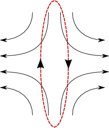
(a) Elongated adjoint ring in shear flow

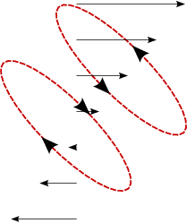
(b) Elongated rings in parallel shear layer

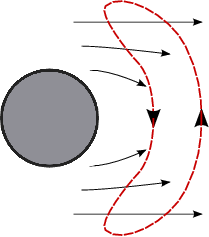
(c) Bean shaped ring in a wake

Figure 1: Amplification of elongated adjoint circulation

The second observation can explain some features of the adjoint fields we observe in the cylinder wake. In particular, a commonly observed structure of the adjoint field is elongated eddies, which often happens in shear flows. Figure 1a illustrates how such eddies are preferentially amplified in shear flow. In this figure, the thin black solid lines represent the fluid velocity, and the thick red dashed lines represent an elongated eddy of the adjoint field. In this flow, fluid particles along the vertical direction are squeezed against each other, while fluid particles along the horizontal direction are stretched. Now consider the production of circulation along the elongated adjoint eddies, as defined in Equation (19). The long, vertical legs of the eddy experience squeezing forwards in time (stretching backwards in time). Therefore, they contribute to amplification of circulation according to (19). The short, horizontal legs of the elongated adjoint eddy experience stretching forwards in time (squeezing backwards in time). They contribute to damping of the adjoint circulation according to (19). Because the horizontal legs are shorter than the vertical legs, the main effect is amplification of adjoint circulation of such adjoint eddies, elongated along the convergent direction of the shear flow.

As an example of the analysis above, consider a parallel shear layer as illustrated in Figure 1b. The flow velocity gradient in the parallel shear layer consists of clockwise rotation (anti-symmetric part of the velocity strain tensor) and a symmetric shear in the 45 degrees direction (symmetric part of the velocity strain tensor). As a result, the adjoint circulation aligned 45 degrees to the shear layer is the most amplified, as shown in Figure 1b. It is worth noting that this amplification effect is non-directional, i.e., it equally amplifies elongated adjoint rings with either positive or negative circulation. Therefore, multiple counter-rotating, parallel elongated adjoint rings can be produced in the same shear layer, as illustrated in Figure 1b.

The elongated adjoint circulation in shear flows, as illustrated in Figure 1, is observed in the adjoint field of cylinder wakes. These adjoint flow patterns can be related to Kelvin-Helmholtz modes in shear flows, because they represent external force patterns to the fluid that have most influence on the flow field, and ultimately the drag on the cylinder. While Kelvin-Helmholtz is a 2D phenomenon, more types of instabilities could occur in three dimensions, potentially causing more patterns to appear in the adjoint field.

It is worth noting that amplification of a pattern in the adjoint field may indicate either modal or non-modal (i.e., transient) growth of perturbations in the flow field (Schmid (2007)). In fact, the adjoint field has been a very effective tool for studying non-modal stability of unsteady flows. The combination of modal and non-modal modes makes the adjoint field very complex, especially in 3D flows.

3 Computational results

The results presented in this section are obtained by discretizing both the Navier-Stokes equation (1) and the continuous form of the adjoint equation (2) with a second order finite volume scheme Ham et al. (2007); Wang (2009). The cylinder diameter is 1; the freestream velocity is $(1,0,0)$; the Reynolds number is set by the viscosity $\nu=1/Re_{D}$. A 2D mesh of about $23,500$ control volumes is used for the $Re_{D}=20$ and $Re_{D}=100$ cases. The $Re_{D}=500$ case is solved with a spanwise extent of 4 cylinder diameters. A total number of 2.06 million control volumes are used for the 3D simulation.

For each case, the Navier-Stokes equation is first solved for sufficiently long time to reach a steady or quasi-steady state at $T_{0}$. The Navier-Stokes equation is then further integrated forwards in time to $T_{1}$; the fluid flow field $\mathbf{u}$ between $T_{0}$ and $T_{1}$ is stored in a dynamic checkpointing scheme Wang et al. (2009). The adjoint field is initialized at $T_{1}$ to $\hat{\mathbf{u}}(x,T_{1})=(0,0,0)$, and integrated backwards in time to $T_{0}$. During the backwards time integration, the fluid flow field $\mathbf{u}$ required by the adjoint integrator is retrieved from the checkpointing scheme. The time length of the adjoint solution $T_{1}-T_{0}$ is 50 for all three cases.

3.1 Adjoint flow field of steady wake at $Re_{D}=20$

At Reynolds number $Re_{D}=20$, the fluid flow is steady and stable. Any small perturbation to the fluid flow field asymptotically decays Noack & Eckelmann (1994). In other words, the dynamical system has negative Lyapunov exponents. In the state space, the steady fluid flow solution is a (zero-dimensional) fixed point attractor. For this flow field, the adjoint solution also quickly settles down to a steady state when integrated backwards in time.

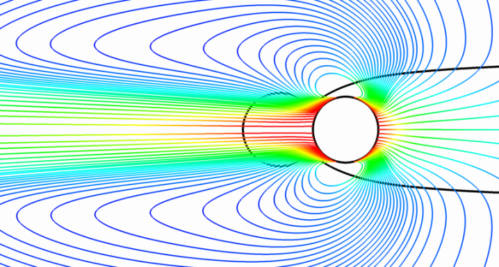
Figure 2: The adjoint velocity field, $Re_{D}=20$. The color indicates the magnitude of the adjoint field $\hat{\mathbf{u}}$. The black lines are contours of streamwise flow velocity at $0$ and $0.8$ freestream velocity.

As shown in Figure 2, the main feature of the adjoint field is a jet of adjoint velocity, generated by the boundary condition $\hat{\mathbf{u}}=(1,0,0)$ at the cylinder surface. The jet propagates upstream while being diffused rapidly by the high viscosity. The adjoint boundary condition of $(1,0,0)$ also applies to the downstream side of the cylinder; the main effect on the downstream is similar to suction. The apparently odd features of the upstream jet and downstream suction is due to the fact that the adjoint evolves backwards in time; thus the directionality of advection is reversed. The jet and suction on the cylinder surface also produce two large eddies on the upper and lower sides of the cylinder.

In this adjoint field, the net adjoint energy production is calculated as $\iiint\hat{P}^{\hat{\mathcal{E}}}\,dV=0.71$, and the net energy dissipation $\iiint\hat{D}^{\hat{\mathcal{E}}}\,dV=1.07$. Because the adjoint field is steady state, the left hand side of the energy balance equation (12) is 0. Therefore, the net loss of energy in the interior of the domain can only be compensated by flux through the boundary. This energy could come from the jet emanating from the front side of the cylinder. We also observe that the magnitude of the adjoint velocity $\hat{\mathbf{u}}$ is almost always less than 1, which is determined by the boundary condition. This may be explained by the dominance of the dissipation term over the production term in the energy balance.

3.2 Adjoint flow field of periodic wake at $Re_{D}=100$

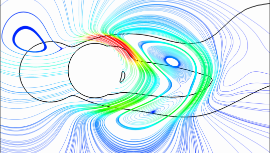
(a) near field, $t=0$

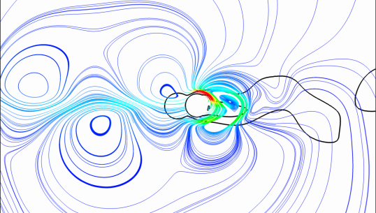
(b) far field, $t=0$

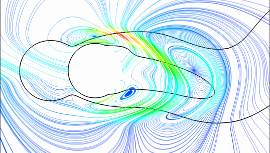
(c) near field, $t=1$

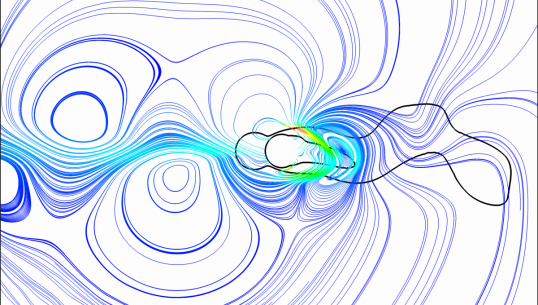
(d) far field, $t=1$

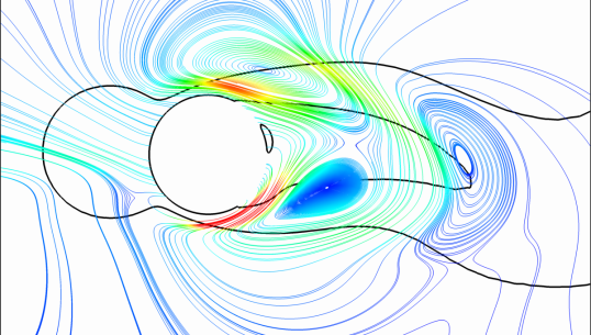
(e) near field, $t=2$

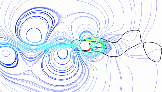
(f) far field, $t=2$

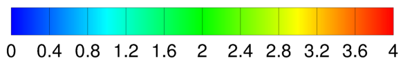
(g)

Figure 3: The adjoint velocity field for about half of a period, $Re_{D}=100$. The color indicates the magnitude of the adjoint field $\hat{\mathbf{u}}$. The black lines are contours of the streamwise flow velocity at $0$ and $0.8$ freestream velocity.

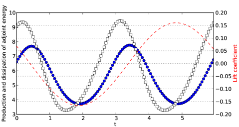
Figure 4: The energy balance of the adjoint field at $Re_{D}=100$. The blue, filled circles represent the net energy production $\iiint\hat{P}^{\hat{\mathcal{E}}}\,dV$; the black, open squares represent the net energy dissipation $\iiint\hat{D}^{\hat{\mathcal{E}}}\,dV$; the red, dashed line is the lift coefficient of the cylinder, which serves to identify the phase of the vortex shedding.

At Reynolds number $Re_{D}=100$, the fluid flow exhibits periodic von Karman vortex shedding. Through Floquet analysis Noack & Eckelmann (1994); Barkley & Henderson (1996), it can be shown that any small perturbation to the periodic fluid flow will asymptotically decay to the periodic state; however, there can be a non-decaying phase difference between the vortex shedding of the unperturbed fluid flow and the perturbed fluid flow, even after the transient disturbance settles down. In other words, the system has a Lyapunov exponent that is exactly equal to 0, and all other Lyapunov exponents are negative. This is a common feature in dynamical systems with a limit cycle attractors. In the state space, the attractor is a one dimensional closed curve. The points on the curve represent time snapshots of the fluid flow. The adjoint field of the periodic flow also settles down to a periodic state in about 2 to 3 shedding periods.

Figure 3 illustrates the evolution of the adjoint field via the stream trace of the adjoint velocity, colored by the adjoint velocity magnitude. The streamwise fluid velocity contours (black) indicate the phase of the vortex shedding and the location of the shear layers. Because the vortex shedding is symmetric, we show three time snapshots covering about half of a period, and the other half of the period is symmetric to the half-period shown. The adjoint field evolves backwards in time, therefore, a good way of examining the dynamics over an entire period is looking at Figures 3e, then 3c and 3a, and then the upside-down versions of Figure 3e, 3c, 3a, in that order. The right column in Figure (3) shows the zoomed-out views of the same adjoint fields.

In Figure 3, the most significant feature in the adjoint field is the bean-shaped eddies behind the cylinder. When viewed backwards in time, these bean-shaped patterns first form at about 2 diameters downstream of the cylinder (Figure 3e), and grow larger and stronger as they propagate upstream in the wake (Figures 3c and 3a). The mechanism responsible for generation and amplification of these bean-shaped eddy structures is described in Section 2.4, and qualitatively depicted in Figure 1c.

The bean-shaped adjoint eddy breaks up into two elongated eddies at about 1 diameter downstream of the cylinder (Figure 3e). Both eddies are aligned in oblique directions to the shear layer. As both eddies approach the cylinder surface, they experience strong dissipation (Figure 3c). One of the two eddies (the lower one in Figure 3c) is trapped in the wake and disappears. The other eddy (the upper one in Figure 3c) propagates upstream of the cylinder in a relatively uniform fluid flow (the upper left eddy in Figure 3a). As these eddies propagate further upstream, they spread out and become more circular by the force of viscosity (Figures 3f, 3d and 3b).

The jet of adjoint velocity in front of the cylinder is still apparent in the adjoint field. It has a magnitude smaller than the adjoint circulation in the wake, and meanders unsteadily between the vortices propagating upstream.

The energy balance of the periodic adjoint field is shown in Figure 4. The net production and dissipation in the interior of the domain have similar magnitudes, and overtake each other twice per period. Averaged over time, the dissipation is slightly more than the self-production of adjoint energy in the interior. This net loss of energy could be compensated by the jet emanating from the cylinder surface.

3.3 Adjoint flow field of turbulent wake at $Re_{D}=500$

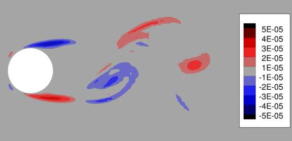
(a) $t=2$

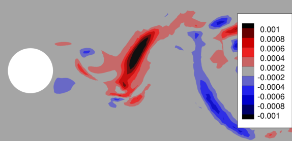
(b) $t=22$

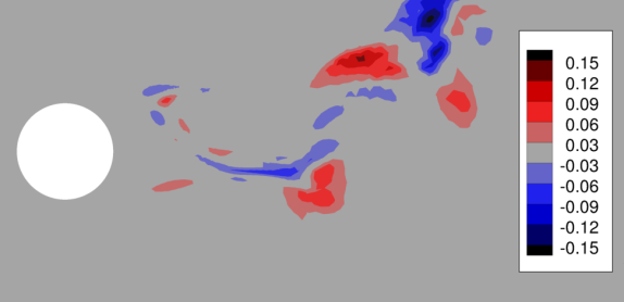
(c) $t=42$

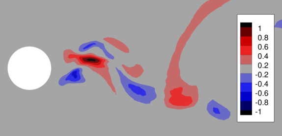
(d) $t=62$

Figure 5: The “butterfly effect” of flow at $Re_{D}=500$. The plots show the difference in spanwise velocity between a perturbed flow field and the unperturbed flow field, at different time snapshots.

At Reynolds number $Re_{D}\approx 189$, a series of complex transitions to turbulence starts. Accurately capturing the unsteady flow field during the transition may require a very large spanwise domain Barkley & Henderson (1996). However, at Reynolds number $Re_{D}=500$, Karniadakis & Triantafyllou (1992) showed that the wake exhibits fully turbulent behavior even with a modest spanwise extent of $\pi$ diameters. In this paper, a spanwise extent of $4$ diameters is used.

In the chaotic, turbulent wake structure, an infinitesimal perturbation could grow exponentially until saturated by nonlinearity. This phenomenon is known as the “butterfly effect”. Figure 5 demonstrates this butterfly effect in the $Re_{D}=500$ case. The four plots show the difference between the spanwise velocity of a perturbed flow field and that of an unperturbed flow field. The unperturbed flow field has been time-integrated to statistical equilibrium at $t=0$; the perturbed flow field is a copy of the unperturbed flow field at $t=0$, plus a perturbation of magnitude $10^{-5}$ at one diameter downstream of the cylinder. Starting from their slightly different initial conditions at $t=0$, the perturbed and unperturbed flow fields are then time-integrated forwards independently, with exactly the same boundary conditions. Figure 5 shows that the difference between the two flow fields, which starts at $10^{-5}$ at $t=0$, grows larger as time progresses. At $t=62$, the difference becomes order 1, as large as the freestream velocity. At that point, the two flow fields are significantly different.

The divergence of a small perturbation is a signature of chaotic dynamics. It implies that almost any quantity that depends on the flow field at a later time, e.g. $t=62$, is very sensitive to almost any small perturbation made at an earlier time, e.g. $t=0$. This has significant implications for the adjoint field, which contains information about sensitivities: the adjoint field at time $t$ indicates sensitivity of an overall quantity of interest to potential perturbations made at $t$. This sensitivity can be very large if the quantity of interest depends on the flow solution at a time much later than $t$, as implied by the butterfly effect of chaos. In our calculation, the quantity of interest embedded in the adjoint equation is an integral over a fixed range of time $[0,T]$; therefore, we expect the adjoint field at time $t$ to be very much larger for $t\ll T$.

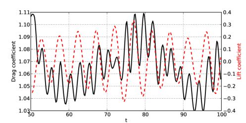
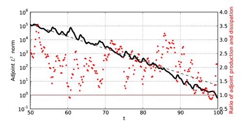
Figure 6: The upper plot shows the lift and drag coefficients as functions of time at $Re_{D}=500$. The lower plot shows the $L^{2}$ norm of the adjoint solution (solid black line), compared to an estimate based on the Lyapunov exponent (dashed line). The ratio of net adjoint energy production and dissipation $\iiint\hat{P}^{\hat{\mathcal{E}}}\,dV/\iiint\hat{D}^{\hat{\mathcal{E}}}\,dV$ is plotted as red dots.

It is indeed observed that the adjoint field has a larger magnitude at smaller $t$. As shown in the lower plot of Figure 6, the magnitude of the adjoint equation increases exponentially as $t$ decreases. This indicates that the quantity of interest is exponentially more sensitive to perturbations at earlier times. This agrees with our observation in Figure 5 that the flow fields at later times are exponentially more sensitive to a perturbation at $t=0$. In addition, the rate at which the adjoint field increases agrees with the Lyapunov exponent, as indicated by the dashed line in Figure 6; the Lyapunov exponent is estimated from the rate at which the perturbed and unperturbed fields diverge (as shown in Figure 5).

The energy balance of the chaotic adjoint field is also shown in Figure 6. The net production in the interior of the domain almost always exceeds the net dissipation, as indicated by the production dissipation ratio. The adjoint energy production in the interior is the main contributor of the exponential growth of the adjoint solution as time goes backwards. This is because the interior energy production term $\hat{P}^{\hat{\mathcal{E}}}$ in Equation (12) is proportional to the squared magnitude of the adjoint solution $\hat{\mathbf{u}}$, while the contribution of energy from the boundary is only proportional to the magnitude of $\hat{\mathbf{u}}$. As the adjoint solution grows larger, the boundary condition becomes less important compared to the interior dynamics.

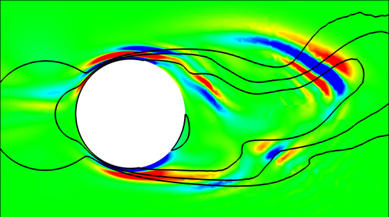
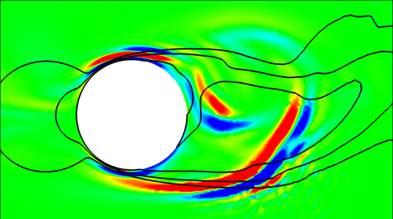
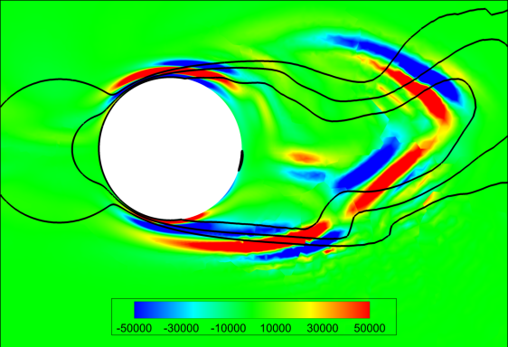
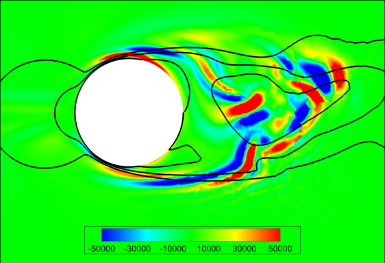
Figure 7: The spanwise component of the adjoint vorticity $\nabla\times\hat{\mathbf{u}}$ at $Re_{D}=500$. The four plots show the spanwise vorticity at different spanwise sections at time $t=T_{1}-38$. The black lines are contours of streamwise flow velocity at $0$, $0.4$ and $0.8$ freestream velocity.

Figure 7 visualizes the diverging adjoint field by plotting the spanwise adjoint vorticity $\nabla\times\hat{\mathbf{u}}$ at four different spanwise sections at $t=T_{1}-38$, i.e., after 38 time units of adjoint time integration. The field concentrates almost entirely in the near-wake region. The adjoint eddies appear in mostly parallel streaks that are oblique to the shear layers in the wake. These structures are consistent with our analysis in Section 2.4, as sketched in Figure 1.

The jet of adjoint velocity in front of the cylinder, a significant feature in the lower Reynolds number cases, is no longer visible. This can be explained by comparing the adjoint energy production in the interior $\hat{P}^{\hat{\mathcal{E}}}$ (Equation (12)) and adjoint energy production on the boundary $\hat{P}^{BC}$ (Equation (13)). As the magnitude of the adjoint field becomes larger, the contribution of energy from the boundary condition increases linearly, while the contribution of energy from the interior production term $\hat{P}^{\hat{\mathcal{E}}}$ increases quadratically. Because the energy of the jet comes from the boundary condition, its magnitude is relatively small when the adjoint field becomes very large.

4 Conclusions

The solution of the adjoint equation with drag being the quantity of interest can be viewed as a nondimensional transfer function of small momentum perturbations. We analyze the solution of the adjoint equation with conventional fluid mechanical methods, including studying the kinetic energy of the adjoint field and the evolution of circulation along a closed material contour. The result of our analysis shows that the adjoint kinetic energy is not conserved; in particular, the adjoint field can exponentially amplify along certain eigen-directions of the flow shear rate tensor $\frac{1}{2}(\nabla\mathbf{u}+\nabla\mathbf{u}^{T})$. Analysis of circulation dynamics reveals that the dynamics of the adjoint equation should preferentially amplify elongated eddies that are aligned with converging directions of a shear flow. In a parallel shear flow, the amplified eddies should be elongated along a 45 degrees angle direction relative to the shear layer.

Numerical solutions of the adjoint equation are performed for a circular cylinder at Reynolds numbers $Re_{D}=20,100$ and $500$. At $Re_{D}=20$, both the flow solution and the adjoint solution are steady. Downstream of the cylinder, the adjoint field has streamlines similar to that of fluid being sucked into the downstream part of the cylinder; upstream of the cylinder, the adjoint field has streamlines similar to that of fluid being ejected towards upstream of the cylinder, forming a jet-like structure. These features in the adjoint field are consistent with the physical interpretation of the adjoint field. At $Re_{D}=100$, both the flow field and the adjoint field are 2D and periodic. We observe bean-shaped eddies in the adjoint field forming in the near-wake region of the cylinder. These eddies form because they are preferentially amplified by the dynamics of the adjoint equation in shear flow. At $Re_{D}=500$, the flow in the wake is turbulent; the entire adjoint field is amplified exponentially as time evolves backwards. This amplification is caused by the production of adjoint energy in the interior dominating viscous dissipation. The rate of exponential amplification is consistent with the Lyapunov exponent of the turbulent flow. The dominant structure in the adjoint field is thin, elongated eddies in the near-wake region, created by preferential amplification of these eddies in the shear layers of the near wake.

Appendix A Derivation of the adjoint equation

The derivation starts with the linearized Navier-Stokes equation (5) that describes the small change in the flow field $\delta\mathbf{u}$ caused by an infinitesimal body force $\delta\mathbf{f}$ in the interior of the flow field. By taking the inner product of the adjoint field $\hat{\mathbf{u}}(x,t)$ with the linearized momentum equation in Equation (5), and multiplying the adjoint pressure $\hat{p}$ with the divergence-free condition in Equation (5), we obtain

$$\begin{split}&\underbrace{\rho\frac{\partial\delta\mathbf{u}}{\partial t}\cdot\hat{\mathbf{u}}}_{(L1)}+\underbrace{\rho\,\mathbf{u}\cdot\nabla\delta\mathbf{u}\,\cdot\hat{\mathbf{u}}}_{(L2)}+\underbrace{\rho\,\delta\mathbf{u}\cdot\nabla\mathbf{u}\,\cdot\hat{\mathbf{u}}}_{(L3)}+\underbrace{\nabla\delta p\,\cdot\hat{\mathbf{u}}}_{(L4)}-\underbrace{\mu\nabla\cdot\nabla\delta\mathbf{u}\,\cdot\hat{\mathbf{u}}}_{(L5)}=\delta\mathbf{f}\,\cdot\hat{\mathbf{u}}\\ &\underbrace{\hat{p}\;\nabla\cdot\delta\mathbf{u}}_{(L6)}=0\end{split}$$ (21)

The adjoint equation (2) is designed to be “symmetric” to the linearized Navier-Stokes equation. By taking the inner product of the velocity field perturbation $\delta u(x,t)$ with the adjoint momentum equation in Equation (2), and multiplying the pressure field perturbation $\delta p$ with the divergence-free condition in Equation (2), we obtain

$$\begin{split}&\underbrace{\rho\frac{\partial\hat{\mathbf{u}}}{\partial t}\cdot\delta\mathbf{u}}_{(A1)}+\underbrace{\rho\,\mathbf{u}\cdot\nabla\hat{\mathbf{u}}\,\cdot\delta\mathbf{u}}_{(A2)}-\underbrace{\rho\,\delta\mathbf{u}\cdot\nabla\mathbf{u}\,\cdot\hat{\mathbf{u}}}_{(A3)\equiv(L3)}+\underbrace{\nabla\hat{p}\,\cdot\delta\mathbf{u}}_{(A6)}+\underbrace{\mu\nabla\cdot\nabla\hat{\mathbf{u}}\,\cdot\delta\mathbf{u}}_{(A5)}=0\\ &\underbrace{\delta p\;\nabla\cdot\hat{\mathbf{u}}}_{(A4)}=0\end{split}$$ (22)

By adding corresponding terms together and integrating over either space or time, we obtain

$$\int_{0}^{T}(L1)+(A1)\,dt=\rho\,\delta\mathbf{u}\cdot\hat{\mathbf{u}}\bigg{|}_{0}^{T}=0$$ (23)

because $\delta\mathbf{u}=0$ at $t=0$ and $\hat{\mathbf{u}}=0$ at $t=T$:

$$\begin{split}\iiint((L2)+(A2))\,dV&=\iiint\rho\,\mathbf{u}\cdot\nabla(\delta\mathbf{u}\cdot\hat{\mathbf{u}})\,dV=\oiint\rho\,(\mathbf{u}\cdot\mathbf{n})(\delta\mathbf{u}\cdot\hat{\mathbf{u}})\,ds\\ \iiint((L4)+(A4))\,dV&=\iiint\nabla\cdot(\delta p\,\hat{\mathbf{u}})\,dV=\oiint\delta p\,(\hat{\mathbf{u}}\cdot\mathbf{n})\,ds\\ \iiint((L6)+(A6))\,dV&=\iiint\nabla\cdot(\hat{p}\,\delta\mathbf{u})\,dV=\oiint\hat{p}\,(\delta\mathbf{u}\cdot\mathbf{n})\,ds\\ \iiint((L5)+(A5))\,dV&=\oiint\mu(\mathbf{n}\cdot\nabla\hat{\mathbf{u}}\,\cdot\delta\mathbf{u}-\mathbf{n}\cdot\nabla\delta\mathbf{u}\,\cdot\hat{\mathbf{u}})\,ds\end{split}$$ (24)

Therefore, by adding equations (21) and (22), we obtain

$$\begin{split}&\int_{0}^{T}\iiint\delta\mathbf{f}\,\cdot\hat{\mathbf{u}}\,dV\,dt\\ =&\int_{0}^{T}\oiint\Big{(}\rho\,(\mathbf{u}\cdot\mathbf{n})(\delta\mathbf{u}\cdot\hat{\mathbf{u}})+\hat{\mathbf{u}}\cdot(\delta p\,\mathbf{n}-\mu\,\mathbf{n}\cdot\nabla\delta\mathbf{u})+\delta\mathbf{u}\cdot(\hat{p}\,\mathbf{n}+\mu\,\mathbf{n}\cdot\nabla\hat{\mathbf{u}})\Big{)}\,ds\;dt\end{split}$$ (25)

For external flow problems, we let the linearized and adjoint Navier-Stokes equations satisfy the boundary conditions

$$\delta{\mathbf{u}}=(0,0,0)\;, \hat{\mathbf{u}}=(1,0,0)\;,$$ at the walls (26)

$$\delta{\mathbf{u}}=(0,0,0)\;, \hat{\mathbf{u}}=(0,0,0)\;,$$ at the far field

For internal flow problems, we enforce a different set of boundary conditions

$$\delta{\mathbf{u}}=(0,0,0)\;, \hat{\mathbf{u}}=(1,0,0)\;,$$ at the walls (27)

$$\rho\,(\mathbf{u}\cdot\mathbf{n})\delta\mathbf{u}+\delta p\,\mathbf{n}-\mu\,\mathbf{n}\cdot\nabla\delta\mathbf{u}=0\;, \mu\,\mathbf{n}\cdot\nabla\hat{\mathbf{u}}+\hat{p}\,\mathbf{n}=0\;,$$ at the inlets

$$\rho\,(\mathbf{u}\cdot\mathbf{n})\hat{\mathbf{u}}+\hat{p}\,\mathbf{n}+\mu\,\mathbf{n}\cdot\nabla\hat{\mathbf{u}}=0\;, \mu\,\mathbf{n}\cdot\nabla\delta\mathbf{u}-\delta p\,\mathbf{n}=0\;,$$ at the outlets

Either set of boundary conditions can be combined with Equation (25) to obtain

$$\int_{0}^{T}\iiint\delta\mathbf{f}\,\cdot\hat{\mathbf{u}}\,dV\,dt\\ =\int_{0}^{T}\int_{S}\hat{\mathbf{u}}\cdot(\delta p\,\mathbf{n}-\mu\,\mathbf{n}\cdot\nabla\delta\mathbf{u})\,ds\;dt=\int_{0}^{T}\delta D\,dt$$ (28)

where $S$ denotes the walls over which the drag is calculated.