Two and four-loop $\beta$-functions of rank 4 renormalizable tensor field theories

Abstract

A recent rank 4 tensor field model generating 4D simplicial manifolds has been proved to be renormalizable at all orders of perturbation theory [arXiv:1111.4997 [hep-th]]. The model is built out of $\phi^{6}$ ($\phi^{6}_{(1/2)}$), $\phi^{4}$ ($\phi^{4}_{(1)}$) interactions and an anomalous term ($\phi^{4}_{(2)}$). The $\beta$-functions of this model are evaluated at two and four loops. We find that the model is asymptotically free in the UV for both the main $\phi^{6}_{(1/2)}$ interactions whereas it is safe in the $\phi^{4}_{(1)}$ sector. The remaining anomalous term turns out to possess a Landau ghost.

Pacs numbers: 11.10.Gh, 04.60.-m, 02.10.Ox
Key words: Renormalization, beta-function, RG flows, tensor models, quantum gravity.
pi-qg-278 and ICMPA/MPA/2012/009

I Introduction

The mid 80’s has witnessed significant developments on quantum gravity (QG) in 2D through matrix models. These models appear to be appropriate candidates achieving a discrete version of the sum of geometries and topologies of surfaces through a sum over random triangulations Di Francesco:1993nw . One of the main tools in order to perform analytically the statistical analysis of these models and their different continuum limits is the $1/N$ expansion of t’Hooft. In the large $N$ (matrix size) limit, only dominate in the partition function planar graphs triangulating surfaces of genus zero. Higher dimensional extensions of these 2D models which were naturally called tensor models with relevance for 3D and 4D gravity, turn out to be a far greater challenge ambj3dqg ; mmgravity ; sasa1 ; Boul ; oriti . The crucial $1/N$ expansion providing a control on the topology of simplices was missing for models generating simplicial manifolds in higher dimensions. In last resort, main results on tensor models then relied on numerics.

Recently important progresses on this latter point have been made. The tensor analogue of the $1/N$ expansion has been found Gur3 ; GurRiv ; Gur4 for a special class of models called colored discovered by Gurau color ; Gurau:2009tz ; Gurau:2010nd . The prominent feature in this expansion is that the dominant contributions in the partition function are dual to spheres thus generalizing surfaces of genus zero in this higher dimensional context (see Gurau:2011xp for a review on colored models). From this breakthrough, one acknowledges interesting achievements on the statistical analysis around tensor models Bonzom:2011zz ; Bonzom:2011ev ; Benedetti:2011nn ; Gurau:2011sk ; Bonzom:2012sz ; Bonzom:2012hw ; Bonzom:2012qx as well as on longstanding mathematical physics questions Gurau:2011tj ; Gurau:2011kk ; Gurau:2012ix . These results have given birth to a new framework, the so-called Tensor Field Theory approach for QG Rivasseau:2011xg ; Rivasseau:2011hm which combines tensor interactions and quantum field theory propagators to formulate a Renormalization Group (RG) based scenario for QG in higher dimensions.

One point should be stressed in a straightforward manner: tensor models of this kind are combinatorial models generating topological spaces and, although they should belong to the scenario of an emergent theory for gravity, their connection with a full-fledged quantization of General Relativity (GR) is not well understood at this stage. Imposing particular conditions on the tensors may convey these models presently discussed closer to what can be expected from a quantization of topological BF theory Boul ; oriti which after further constraints leads to the quantization of GR. Hence, the deeper understanding of these models could be useful for the randomization of geometry. Besides, they possess a number of interesting properties worthy to be studied in details. Indeed, in addition of all important features aforementioned, this class of tensor models generates, in the correct truncation and for the first time, a renormalizable theory for quantum topology in 3 and 4D arXiv:1111.4997 ; BenGeloun:2012pu .

The model considered in arXiv:1111.4997 is a dynamical rank 4 tensor model over $T_{4}\equiv U(1)^{4}$ built with $\phi^{6}$ and $\phi^{4}$ interactions (including one anomalous term). It addresses the generation of 4D simplicial (pseudo-)manifolds in an Euclidean path integral formalism. The three ingredients of perturbative renormalization at all orders Rivasseau:1991ub have been identified: (1) A multi-scale analysis showed that slices can be understood as in the ordinary situation: high scales mean high momenta meaning small distances on the torus; (2) A power counting theorem generalizing known power countings for the local $\phi^{4}_{4}$ and the $\phi^{4}$ Grosse-Wulkenhaar matrix model Grosse:2004yu ; Rivasseau:2007ab and (3) a generalized locality principle yielding a characterization of the most divergent contributions which are of the form of terms included in the initial Lagrangian. A rank 3 analogue model was investigated in BenGeloun:2012pu . This last model also proves to be renormalizable at all orders and, by computing its one-loop $\beta$-function, turns out to asymptotically free in the UV. In other words, the latter statement claims that, in the UV limit, the theory describes the dynamics of non interacting three dimensional objects with the sphere topology.

In this work, we investigate the $\beta$-functions related to all coupling constants of the 4D model defined in arXiv:1111.4997 . Two-loop computations are sufficient for some couplings whereas, for some other couplings, four-loop calculations are required in order to understand the UV behaviour of the model. One needs to go beyond one-loop calculations in order to understand the RG flows due to the presence of the $\phi^{6}$ nonlocal interactions. We prove that the model is asymptotically free in the UV that is, there exists a UV fixed manifold associated with this theory defined by

$$\lambda_{6}=0\qquad\qquad\forall\lambda_{4;1}\quad\qquad\lambda_{4;2}=0$$ (1)

where $\lambda_{6}$ represents any coupling constant of the $\phi^{6}$ interactions, $\lambda_{4;1}$ represents any coupling constant of the $\phi^{4}$ interactions and $\lambda_{4;2}$ the coupling constant the anomalous term of the form $(\phi^{2})^{2}$. Perturbing the system around this fixed manifold

$$\lambda^{\prime}_{6}=\lambda_{6}+\epsilon\qquad\forall\lambda_{4;1}\qquad\lambda^{\prime}_{4;2}=\lambda_{4;2}+\epsilon^{\prime}$$ (2)

for small quantities $\epsilon$ and $\epsilon^{\prime}$, then $\lambda^{\prime}_{6}$, $\lambda_{4;1}$ and $\lambda^{\prime}_{4;2}$ increase in the infrared (IR). These are the main results of this paper.

The plan of this paper is as follows: The next section presents the model and reviews its power counting theorem. Section III investigates in details the two and four-loop $\beta$-functions of the enlarged model incorporating fourteen plus one different couplings associated with all interactions. A conclusion follows in Section IV and an appendix gathers the proofs of different lemmas and important steps in the calculations.

II The model and its renormalizability: An overview

This section yields, in a streamlined analysis, a review of the model as defined in arXiv:1111.4997 and its power counting theorem which will be used at each step of the rest of the paper.

Let us consider a fourth rank complex tensor field over the group $U(1)$, $\varphi:U(1)^{4}\to\mathbb{C}$. This field can be decomposed in Fourier modes as

$$\varphi(h_{1},h_{2},h_{3},h_{4})=\sum_{p_{j}\in\mathbb{Z}}\varphi_{[p_{j}]}e^{ip_{1}\theta_{1}}e^{ip_{2}\theta_{2}}e^{ip_{3}\theta_{3}}e^{ip_{4}\theta_{4}}$$ (3)

where the group elements $h_{i}\in U(1)$, $\theta_{i}\in[0,2\pi)$ and $[p_{j}]=[p_{1},p_{2},p_{3},p_{4}]$ are momentum indices. We will adopt the notation $\varphi_{[p_{1},p_{2},p_{3},p_{4}]}=$ $\varphi_{1,2,3,4}$. Note that no symmetry under permutation of arguments is assumed for the tensor $\varphi_{[p_{j}]}$.

The action is defined by the kinetic term given in momentum space as

$$S^{\text{kin\,},0}=\sum_{p_{j}}\bar{\varphi}_{1,2,3,4}\Big{(}\sum_{s=1}^{4}(p_{s})^{2}+m^{2}\Big{)}\varphi_{1,2,3,4}$$ (4)

where the sum is performed over all momentum values $p_{j}$. Clearly, such a kinetic term is inferred from a Laplacian dynamics acting on the strand index $s$. It could be interesting to find in which sense the above Laplacian dynamics might be related to an Osterwalder-Schrader positivity axiom vinc . Other motivations on the introduction of such a kinetic term can be found in Geloun:2011cy . The corresponding Gaussian measure of covariance $C=(\sum_{s}p^{2}_{s}+m^{2})^{-1}$ is noted as $d\mu_{C}$.

The interactions of the model are effective interaction terms obtained after color integration Gurau:2011tj . They can be equivalently defined from unsymmetrized tensors as trace invariant objects Gurau:2012ix . The renormalization requires to keep relevant to marginal terms so that only the following monomials of order six at most will be significant

$$S_{6;1} = \sum_{p_{j}}\varphi_{1,2,3,4}\bar{\varphi}_{1^{\prime},2,3,4}\varphi_{1^{\prime},2^{\prime},3^{\prime},4^{\prime}}\bar{\varphi}_{1^{\prime\prime},2^{\prime},3^{\prime},4^{\prime}}\varphi_{1^{\prime\prime},2^{\prime\prime},3^{\prime\prime},4^{\prime\prime}}\bar{\varphi}_{1,2^{\prime\prime},3^{\prime\prime},4^{\prime\prime}}+\text{permutations }$$ (5)

$$S_{6;2} = \sum_{p_{j}}\varphi_{1,2,3,4}\bar{\varphi}_{1^{\prime},2^{\prime},3^{\prime},4}\varphi_{1^{\prime},2^{\prime},3^{\prime},4^{\prime}}\bar{\varphi}_{1^{\prime\prime},2,3,4^{\prime}}\varphi_{1^{\prime\prime},2^{\prime\prime},3^{\prime\prime},4^{\prime\prime}}\bar{\varphi}_{1,2^{\prime\prime},3^{\prime\prime},4^{\prime\prime}}+\text{permutations }$$ (7)

$$S_{4;1} = \sum_{p_{j}}\varphi_{1,2,3,4}\,\bar{\varphi}_{1^{\prime},2,3,4}\,\varphi_{1^{\prime},2^{\prime},3^{\prime},4^{\prime}}\,\bar{\varphi}_{1,2^{\prime},3^{\prime},4^{\prime}}+\text{permutations }$$ (8)

where the sum is over all 24 permutations of the four color indices giving rise to the present model. Note that several configurations have to be moded out from these 24 permutations due to both the momentum summations and the vertex color symmetry. At the end, one ends up with the following:

1. 4 inequivalent vertex configurations appearing in $S_{6;1}$ and $S_{4;1}$; these will be parameterized by an index $\rho=1,2,3,4$ (see Figure 2, top, for the set of vertices in $S_{6;1}$ and Figure 3, top, for those which should appear in $S_{4;1}$);

2. 6 inequivalent vertex configurations in $S_{6;2}$; each of these will be parameterized by a double index $\rho\rho^{\prime}=12,13,14,23,24,34$ (see Figure 2, bottom).

Feynman graphs have a tensor structure that we describe now. Fields are represented by half lines with four strands and propagators are lines with the same structure, see Figure 1.

Figure 1: The propagator.

Vertices become nonlocal objects (see Figure 2 and Figure 3). Simplified diagrams will be often used for simplicity.

Figure 2: Vertices of the type $\phi^{6}_{(1)}$ (top, parametrized by $\rho=1,\dots,4$) and of the type $\phi^{6}_{(2)}$ (bottom, parametrized by $\rho\rho^{\prime}=12,\dots,34$).

Figure 3: Vertices of the type $\phi^{4}_{(1)}$ (parameterized by permutations $\rho=1,2,3,4$) and the anomalous term $\phi^{4}_{(2)}=(\phi^{2})^{2}$ (bottom).

The renormalization analysis prescribes to add to the action another $\phi^{4}$ type interaction that we will refer to as anomalous term of the form

$$S_{4;2}=\left[\sum_{p_{j}}\bar{\varphi}_{1,2,3,4}\,\varphi_{1,2,3,4}\right]\left[\sum_{p^{\prime}_{j}}\bar{\varphi}_{1^{\prime},2^{\prime},3^{\prime},4^{\prime}}\,\varphi_{1^{\prime},2^{\prime},3^{\prime},4^{\prime}}\right]$$ (9)

Such a term can be generated, for instance, by a contraction from a vertex of the $\phi^{6}_{(2)}$ type and can be seen as two factorized $\phi^{2}$ vertices (see Figure 3).

An ultraviolet cutoff $\Lambda$ on the propagator is introduced such that $C$ becomes $C^{\Lambda}$. As in ordinary quantum field theory, bare and renormalized couplings, the difference of which are coupling constant counterterms denoted by $CT$ are introduced. Counterterms $S_{2;1}$ and $S_{2;2}$ should be also introduced in the bare action to perform the mass and wave function renormalization, respectively. The propagator $C$ includes the renormalized mass $m^{2}$ and the renormalized wave function $1$.

The action of the model is then defined as

$$S^{\Lambda}=\lambda^{\Lambda}_{6;1}S_{6;1}+\lambda^{\Lambda}_{6;2}S_{6;2}+\lambda^{\Lambda}_{4;1}S_{4;1}+\lambda^{\Lambda}_{4;2}S_{4;2}+CT^{\Lambda}_{2;1}S_{2;1}+CT^{\Lambda}_{2;2}S_{2;2}$$ (10)

and the partition function is

$$Z=\int d\mu_{C^{\Lambda}}[\varphi]\;e^{-S^{\Lambda}}$$ (11)

We can define four renormalized coupling constants $\lambda^{\text{ren}}_{6;1},\lambda^{\text{ren}}_{6;2},\lambda^{\text{ren}}_{4;1}$ and $\lambda^{\text{ren}}_{4;2}$ such that, choosing appropriately 6 counterterms, the power series expansion of any Schwinger function of the model expressed in powers of the renormalized couplings has a finite limit when removing the cut-off at all orders. This statement has been proved in arXiv:1111.4997 by a multiscale analysis Rivasseau:1991ub and the fine study of the graph topology.

A central point in the proof of the renormalizability is the reintroduction of colors in order to get a useful bound on the graph amplitude. A graph ${\mathcal{G}}$ admits a color extension $\mathcal{G}_{\text{color}}$ (obtained uniquely by restoration of colors) which is itself a rank four tensor graph. The next stage is to define ribbon subgraphs lying inside the tensor graph structure and also the notion of boundary graph encoding mainly the external data.

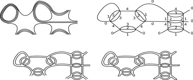
Figure 4: A graph ${\mathcal{G}}$, its colored extension $\mathcal{G}_{\text{color}}$ (five valence vertices with colored (half-)lines), the jacket subgraph $J$ $(01234)$ of $\mathcal{G}_{\text{color}}$ and its associated pinched jacket ${\widetilde{J}}$.

Figure 5: The boundary ${\partial\mathcal{G}}$ of ${\mathcal{G}}$ (see Fig.4) and its rank 3 tensor structure.

Definition 1.

Let ${\mathcal{G}}$ be a graph in the rank $4$ theory.

1. We call colored extension of ${\mathcal{G}}$ the unique graph $\mathcal{G}_{\text{color}}$ obtained after restoring in ${\mathcal{G}}$ the former colored theory graph (see Fig.4).

2. A jacket $J$ of $\mathcal{G}_{\text{color}}$ is a ribbon subgraph of $\mathcal{G}_{\text{color}}$ defined by a color cycle $(0abcd)$ up to a cyclic permutation (see Fig.4). There are 12 such jackets in $D=4$ GurRiv .

3. The jacket ${\widetilde{J}}$ is the jacket obtained from $J$ after “pinching” viz. the procedure consisting in closing all external legs present in $J$ (see Fig.4). Hence it is always a vacuum graph.

4. The boundary ${\partial\mathcal{G}}$ of the graph ${\mathcal{G}}$ is the closed graph defined by vertices corresponding to external legs and by lines corresponding to external strands of ${\mathcal{G}}$ Gurau:2009tz (see Fig.5). It is, in the present case, a vacuum graph of the $3$ dimensional colored theory.

5. A boundary jacket $J_{\partial}$ is a jacket of ${\partial\mathcal{G}}$. There are 3 such boundary jackets in $D=4$.

Consider a connected graph ${\mathcal{G}}$. Let $V_{6}$ be its number of $\phi^{6}$ vertices (of any type) and $V_{4}$ its number of $\phi^{4}_{(1)}$ vertices, $V_{4}^{\prime}$ its number of vertices of type $\phi^{4}_{(2)}=(\phi^{2})^{2}$, $V_{2}$ the number of vertices of the type $\phi^{2}$ (mass counterterms) and $V^{\prime}_{2}$ the number of vertices of the type $(\nabla\phi)^{2}$ (wave function counterterms). Let $L$ be its number of lines and $N_{\text{ext\,}}$ its number of external legs. Consider also its colored extension $\mathcal{G}_{\text{color}}$ and its boundary ${\partial\mathcal{G}}$.

Vertices contributing to $V_{4}^{\prime}$ are disconnected from the point of view of their strands. We reduce them in order to find the power counting with respect to only connected component graphs. These types of vertices will be therefore considered as a pair of two 2-point vertices $V_{2}^{\prime\prime}$, hence $V^{\prime\prime}_{2}=2V_{4}^{\prime}$.

The renormalizability proof involves a power counting theorem based on a multi-scale analysis. For simplicity here and without loss of generality, we use the following monoscale power counting: the amplitude of any connected (with respect to $V_{2}^{\prime\prime}$ and not to $V_{4}^{\prime}$) graph ${\mathcal{G}}$ is bounded by $KM^{i\omega_{d}({\mathcal{G}})}$, where $K$ is a constant and $\omega_{d}({\mathcal{G}})$ is called the divergence degree of ${\mathcal{G}}$ which is an integer and can be written

$$\omega_{d}({\mathcal{G}})=-\frac{1}{3}\left[\sum_{J}g_{{\widetilde{J}}}-\sum_{J_{\partial}}g_{J_{\partial}}\right]-(C_{{\partial\mathcal{G}}}-1)-V_{4}-2(V_{2}+V_{2}^{\prime\prime})-\frac{1}{2}\left[N_{\text{ext\,}}-6\right]$$ (12)

where $g_{{\widetilde{J}}}$ and $g_{J_{\partial}}$ are the genus of ${\widetilde{J}}$ and $J_{\partial}$, respectively, $C_{{\partial\mathcal{G}}}$ is the number of connected components of the boundary graph ${\partial\mathcal{G}}$; the first sum is performed on all closed jackets ${\widetilde{J}}$ of $\mathcal{G}_{\text{color}}$ and the second sum is performed on all boundary jackets $J_{\partial}$ of ${\partial\mathcal{G}}$.

The detailed study of the $\omega_{d}({\mathcal{G}})$ yields a classification of all diverging contributions participating to the RG flow of coupling constants. It occurs that $\omega_{d}({\mathcal{G}})$ does not depend on $V_{6}$. One obtains the following table listing all primitively divergent graphs:

$N_{\text{ext\,}}$	$V_{2}+V_{2}^{\prime\prime}$	$V_{4}$	$\sum_{J_{\partial}}g_{J_{\partial}}$	$C_{{\partial\mathcal{G}}}-1$	$\sum_{{\widetilde{J}}}g_{{\widetilde{J}}}$	$\omega_{d}({\mathcal{G}})$
6	0	0	0	0	0	0
4	0	0	0	0	0	1
4	0	1	0	0	0	0
4	0	0	0	1	0	0
2	0	0	0	0	0	2
2	0	1	0	0	0	1
2	0	2	0	0	0	0
2	0	0	0	0	6	0
2	1	0	0	0	0	0

Table 1: List of primitively divergent graphs

Since $V_{2}^{\prime\prime}=2V_{4}^{\prime}$ is always even, the last row of the table can be forgotten because it mainly involve a graph as a pure mass renormalization.

Call graphs satisfying $\sum_{{\widetilde{J}}}g_{{\widetilde{J}}}=0$ “melonic” graphs or simply “melons” Bonzom:2011zz . Thus, in Table 1, some graphs are melons with melonic boundary, namely those for which also holds $\sum_{J_{\partial}}g_{J_{\partial}}=0$. We are now in position to address the computation of the $\beta$-functions of the model.

III $\beta$-functions at two and four loops

The computation of the $\beta$-functions in this model turns out to be very involved. The method used in this work, though somehow lengthy, is efficient enough to deal with a large number of Feynman graphs and give a precise result.

We shall enlarge the space of couplings by assigning to each interaction in (7), (8) and (9) a different coupling. Only at the end, we will reduce this space of coupling in order to have the UV behavior of some reduced models. We emphasize that, at this level, this can be viewed as an artefact in order to distinguish the different configuration contributing to each of the renormalized coupling constant equation. In short, the combinatorics of the graph configurations can be better addressed in the different coupling setting. From the point of view of renormalization, the extended model with different coupling constants for interactions can be shown to be renormalizable, if at the same time, we enlarge the space of wave function couplings (see the discussion in Subsection 5.3 in BenGeloun:2012pu which addresses this issue for a similar tensor model).

First, we associate to each interaction a different coupling constant such that the total interaction part (without counterterms and omitting to write the cut-off) becomes after having introduced a symmetry factor for interactions in $S_{6;1}$ and $S_{4;1/2}$:

$$S=\frac{1}{3}\sum_{\rho}\lambda_{6;1;\rho}\,S_{6;1;\rho}+\sum_{\rho\rho^{\prime}}\lambda_{6;2;\rho\rho^{\prime}}\,S_{6;2;\rho\rho^{\prime}}+\frac{1}{2}\sum_{\rho}\lambda_{4;1;\rho}\,S_{4;1;\rho}+\frac{1}{2}\lambda_{4;2}\,S_{4;2}$$ (13)

where $\rho$ and $\rho\rho^{\prime}$ are permutations of indices as given in Figure 2 and Figure 3. Mainly, there are 4 terms in the sum involving $S_{6;1;\rho}$, in the second sum involving $S_{6;2;\rho\rho^{\prime}}$, there are 6 terms and, in the last regarding $S_{4;1;\rho}$, the sum is also performed over 4 terms. Note that in the following, we always consider $\lambda_{6;2;\rho\rho^{\prime}}=\lambda_{6;2;\rho^{\prime}\rho}$ and $\rho\neq\rho^{\prime}$.

We are mainly interested in the behaviour of the renormalized coupling coupling constants $\lambda^{\text{ren\,}}_{6;\xi;\rho/\rho\rho^{\prime}}$, $\lambda^{\text{ren\,}}_{4;1;\rho}$ and $\lambda^{\text{ren\,}}_{4;2}$ in the UV. In fact, the determination of the $\beta$-functions of the $\phi^{6}_{(\xi)}$ vertices, $\xi=1,2$, turns out to be crucial for the entire analysis.

Any $\beta$-function, at a certain number of loops, is generally computed after the determination of two ingredients: the wave function renormalization and the truncated and amputated one particle irreducible (1PI) $N$-point function the external data of which are designed in the form of the initial (bare) interaction. In the present situation, the wave function renormalization $Z$ can be written as

$$Z=1-\partial_{b_{1}^{2}}\;\Sigma\;\Big{|}_{b_{1,2,3,4}=0}\qquad\quad\Sigma(b_{1},b_{2},b_{3},b_{4})=\big{\langle}\varphi_{1,2,3,4}\bar{\varphi}_{1,2,3,4}\big{\rangle}^{t}_{1PI}\qquad\quad\varphi_{1,2,3,4}=\varphi_{b_{1},b_{2},b_{3},b_{4}}$$ (14)

where $b_{i}$ are external momenta and $\Sigma$ is the so-called self-energy or sum of all amputated 1PI two-point functions. The latter will be computed at two loops at first. Note that $\Sigma$ should be symmetric in its arguments so that the above derivative with respect to $b_{1}^{2}$ can be replaced by any derivative with respect to another argument without loss of generality.

The $\beta$-functions related to the running of coupling constants are encoded in the following ratios:

$$\lambda_{6;\xi;\rho/\rho\rho^{\prime}}^{\text{ren\,}} = -\frac{\Gamma_{6;\xi;\rho/\rho\rho^{\prime}}(0,0,0,0,0,0,0,0,0,0,0,0)}{Z^{3}}\qquad\quad\lambda_{4;1;\rho}^{\text{ren\,}}=-\frac{\Gamma_{4;1;\rho}(0,0,0,0,0,0,0,0)}{Z^{2}}$$ (15)

$$\lambda_{4;2}^{\text{ren\,}} = -\frac{\Gamma_{4;2}(0,0,0,0,0,0,0,0)}{Z^{2}}$$ (17)

where $\Gamma_{6;\xi;\rho/\rho\rho^{\prime}}(b_{1},b_{2},b_{3},b_{4},b_{1}^{\prime},b_{2}^{\prime},b_{3}^{\prime},b_{4}^{\prime},b_{1}^{\prime\prime},b_{2}^{\prime\prime},b_{3}^{\prime\prime},b_{4}^{\prime\prime})$ is the sum of amputated 1PI six-point functions or corrections to one of the $\phi^{6}_{(\xi)}$ vertices with coupling constant $\lambda_{6;\xi;\rho/\rho\rho^{\prime}}$ and $\Gamma_{4;1;\rho}(b_{1},b_{2},b_{3},b_{4},b_{1}^{\prime},b_{2}^{\prime},b_{3}^{\prime},b_{4}^{\prime})$ the sum of amputated 1PI four-point functions, corrections to one of the vertex $\phi^{4}_{(1)}$ with coupling constant $\lambda_{4;1;\rho}$. The same holds for the last $\phi^{4}_{(2)}$ interaction. For instance, for particular vertices $\phi^{6}_{(1);\rho=1}$, $\phi^{6}_{(2);\rho\rho^{\prime}=14}$ and $\phi^{4}_{(1);\rho=1}$, we have

$$\Gamma_{6;1;\rho=1}(b_{1},b_{2},b_{3},b_{4},b_{1}^{\prime},b_{2}^{\prime},b_{3}^{\prime},b_{4}^{\prime},b_{1}^{\prime\prime},b_{2}^{\prime\prime},b_{3}^{\prime\prime},b_{4}^{\prime\prime})=\langle\,\varphi_{1,2,3,4}\,\bar{\varphi}_{1^{\prime},2,3,4}\,\varphi_{1^{\prime},2^{\prime},3^{\prime},4^{\prime}}\,\bar{\varphi}_{1^{\prime\prime},2^{\prime},3^{\prime},4^{\prime}}\,\varphi_{1^{\prime\prime},2^{\prime\prime},3^{\prime\prime},4^{\prime\prime}}\,\bar{\varphi}_{1,2^{\prime\prime},3^{\prime\prime},4^{\prime\prime}}\,\rangle^{t}_{1PI}$$ (18)

(19)

$$\Gamma_{6;2;\rho\rho^{\prime}=14}(b_{1},b_{2},b_{3},b_{4},b_{1}^{\prime},b_{2}^{\prime},b_{3}^{\prime},b_{4}^{\prime},b_{1}^{\prime\prime},b_{2}^{\prime\prime},b_{3}^{\prime\prime},b_{4}^{\prime\prime})=\langle\,\varphi_{1,2,3,4}\,\bar{\varphi}_{1^{\prime},2^{\prime},3^{\prime},4}\,\varphi_{1^{\prime},2^{\prime},3^{\prime},4^{\prime}}\,\bar{\varphi}_{1^{\prime\prime},2,3,4^{\prime}}\,\varphi_{1^{\prime\prime},2^{\prime\prime},3^{\prime\prime},4^{\prime\prime}}\,\bar{\varphi}_{1,2^{\prime\prime},3^{\prime\prime},4^{\prime\prime}}\,\rangle^{t}_{1PI}$$ (20)

(21)

$$\Gamma_{4;1;\rho=1}(b_{1},b_{2},b_{3},b_{4},b_{1}^{\prime},b_{2}^{\prime},b_{3}^{\prime},b_{4}^{\prime})=\langle\,\varphi_{1,2,3,4}\,\bar{\varphi}_{1^{\prime},2,3,4}\,\varphi_{1^{\prime},2^{\prime},3^{\prime},4^{\prime}}\,\bar{\varphi}_{1,2^{\prime},3^{\prime},4^{\prime}}\,\rangle^{t}_{1PI}$$ (22)

(23)

$$\Gamma_{4;2}(b_{1},b_{2},b_{3},b_{4},b_{1}^{\prime},b_{2}^{\prime},b_{3}^{\prime},b_{4}^{\prime})=\langle\,\varphi_{1,2,3,4}\,\bar{\varphi}_{1,2,3,4}\,\varphi_{1^{\prime},2^{\prime},3^{\prime},4^{\prime}}\,\bar{\varphi}_{1^{\prime},2^{\prime},3^{\prime},4^{\prime}}\,\rangle^{t}_{1PI}$$ (24)

The remaining cases indexed by $\rho$ and $\rho\rho^{\prime}$ can be easily inferred by permutations. Note that the choice of particular external momentum data is justified by the renormalization prescription.

The main results of this paper are captured by the following statements:

Theorem 1.

At two loops, the renormalized coupling constants satisfy the equations

$$\lambda^{\text{ren\,}}_{6;1;\rho} = \lambda_{6;1;\rho}-6\lambda_{6;1;\rho}\Big{[}\lambda_{6;1;\rho}-\lambda_{6;1;1}\Big{]}\,S^{1}-3\lambda_{6;1;\rho}\Big{[}\sum_{\rho^{\prime}\in\{2,3,4\}\setminus\{\rho\}}\Big{(}\lambda_{6;2;\rho\rho^{\prime}}-\lambda_{6;2;1\rho^{\prime}}\Big{)}\Big{]}[S^{1}+S^{12}]+O(\lambda^{3})$$ (25)

$$\lambda_{6;2;\rho\rho^{\prime}}^{\text{ren\,}} = \lambda_{6;2;\rho\rho^{\prime}}-2\lambda_{6;2;\rho\rho^{\prime}}[\lambda_{6;1;\rho}+\lambda_{6;1;\rho^{\prime}}-3\lambda_{6;1;1}]S^{1}-\lambda_{6;2;\rho\rho^{\prime}}\Bigg{[}-\sum_{\bar{\rho}=2,3,4}\lambda_{6;2;1\bar{\rho}}$$ (26)

$$+ \sum_{\bar{\rho}\in\{2,3,4\}\setminus\{\rho\}}(\lambda_{6;2;\rho\bar{\rho}}-\lambda_{6;2;1\bar{\rho}})+\sum_{\bar{\rho}\in\{2,3,4\}\setminus\{\rho^{\prime}\}}(\lambda_{6;2;\rho^{\prime}\bar{\rho}}-\lambda_{6;2;1\bar{\rho}})\Bigg{]}[S^{1}+S^{12}]+O(\lambda^{3})$$ (27)

$$S^{1} := \sum_{p_{1},\dots,p_{6}}\frac{1}{(p_{1}^{2}+p_{2}^{2}+p_{3}^{2}+m^{2})^{2}}\frac{1}{(p_{4}^{2}+p_{5}^{2}+p_{6}^{2}+m^{2})}$$ (29)

$$S^{12} := \sum_{p_{1},\dots,p_{6}}\frac{1}{(p_{1}^{2}+p_{2}^{2}+p_{3}^{2}+m^{2})^{2}}\frac{1}{(p_{1}^{2}+p_{4}^{2}+p_{5}^{2}+p_{6}^{2}+m^{2})}$$ (30)

where $S^{1}$ and $S^{12}$ are formal log-divergent sums, $\rho,\rho^{\prime}\in\{1,2,3,4\}$, $\rho^{\prime}\neq\rho$, and $O(\lambda^{3})$ denotes a sum of O-functions with arguments any cubic power of the coupling constants $O(\lambda_{6;1;\bullet}^{3})+O(\lambda_{6;1;\bullet}^{2}\lambda_{6;2;\bullet})+O(\lambda_{6;1;\bullet}\lambda_{6;2;\bullet}^{2})+O(\lambda_{6;2;\bullet}^{3})$.

Theorem 2.

At a vanishing bare value of all $\lambda_{6;2;\rho\rho^{\prime}}$, the renormalized coupling constants at four loops for the $\phi^{6}_{(1)}$ sector satisfy the equations

$$\lambda_{6;1;\rho}^{\text{ren\,}} = \lambda_{6;1;\rho}+6\lambda_{6;1;\rho}[\lambda_{6;1;1}-\lambda_{6;1;\rho}]S^{1}+\lambda_{6;1;\rho}\Bigg{\{}4\Big{[}5\lambda_{6;1;\rho}^{2}-3\lambda_{6;1;1}^{2}\Big{]}{\mathcal{S}}^{1}_{(1)}+6\Big{[}5\lambda_{6;1;\rho}^{2}+\lambda_{6;1;1}^{2}-6\lambda_{6;1;1}\lambda_{6;1;\rho}\Big{]}{\mathcal{S}}^{1}_{(2)}\Bigg{\}}$$ (32)

$$+6\lambda_{6;1;\rho}\Bigg{[}\lambda_{6;1;\rho}\sum_{\rho^{\prime}\neq\rho}\lambda_{6;1;\rho^{\prime}}-\lambda_{6;1;1}\sum_{\rho^{\prime}=2,3,4}\lambda_{6;1;\rho^{\prime}}\Bigg{]}\Big{[}2{\mathcal{S}}^{12}_{(1)}+{\mathcal{S}}^{12}_{(2)}\Big{]}+O(\lambda^{4})$$

where $O(\lambda^{4})$ denotes a $O$-function involving any quartic product of coupling constants and where

$${\mathcal{S}}^{1}_{(1)} := \sum_{p_{1},\dots,p_{12}}\Big{[}\frac{1}{(p_{1}^{2}+p_{2}^{2}+p_{3}^{2}+m^{2})^{3}}\frac{1}{(p_{4}^{2}+p_{5}^{2}+p_{6}^{2}+m^{2})}\frac{1}{(p_{7}^{2}+p_{8}^{2}+p_{9}^{2}+m^{2})}\frac{1}{(p_{10}^{2}+p_{11}^{2}+p_{12}^{2}+m^{2})}\Big{]}$$ (33)

$${\mathcal{S}}^{1}_{(2)} := \sum_{p_{1},\dots,p_{12}}\Big{[}\frac{1}{(p_{1}^{2}+p_{2}^{2}+p_{3}^{2}+m^{2})^{2}}\frac{1}{(p_{4}^{2}+p_{5}^{2}+p_{6}^{2}+m^{2})^{2}}\frac{1}{(p_{7}^{2}+p_{8}^{2}+p_{9}^{2}+m^{2})}\frac{1}{(p_{10}^{2}+p_{11}^{2}+p_{12}^{2}+m^{2})}\Big{]}$$ (34)

$${\mathcal{S}}^{12}_{(1)} := \sum_{p_{1},\dots,p_{12}}\Big{[}\frac{1}{(p_{1}^{2}+p_{2}^{2}+p_{3}^{2}+m^{2})^{3}}\frac{1}{(p_{1}^{2}+p_{4}^{2}+p_{5}^{2}+p_{6}^{2}+m^{2})}\frac{1}{(p_{1}^{2}+p_{7}^{2}+p_{8}^{2}+p_{9}^{2}+m^{2})}\times$$ (36)

$$\frac{1}{(p_{10}^{2}+p_{11}^{2}+p_{12}^{2}+m^{2})}\Big{]}$$

$${\mathcal{S}}^{12}_{(2)} := \sum_{p_{1},\dots,p_{12}}\Big{[}\frac{1}{(p_{1}^{2}+p_{2}^{2}+p_{3}^{2}+m^{2})^{2}}\frac{1}{(p_{1}^{2}+p_{4}^{2}+p_{5}^{2}+p_{6}^{2}+m^{2})}\frac{1}{(p_{1}^{2}+p_{7}^{2}+p_{8}^{2}+p_{9}^{2}+m^{2})}\times$$ (38)

$$\frac{1}{(p_{10}^{2}+p_{11}^{2}+p_{12}^{2}+m^{2})^{2}}\Big{]}$$

Corollary 1.

At a vanishing bare value of all $\lambda_{6;2;\rho\rho^{\prime}}$ and at two loops, the renormalized coupling constants associated with the $\phi^{4}$ interactions satisfy the equations

$$\lambda^{\text{ren\,}}_{4;1;\rho}=\lambda_{4;1;\rho}$$ (39)

$$\lambda^{\text{ren\,}}_{4;2}=\lambda_{4;2}-\lambda_{4;2}^{2}\,S^{\prime 0}+O(\lambda_{4;2}^{3})\qquad\qquad S^{\prime 0}=\sum_{p_{1},\dots,p_{4}}\frac{1}{(p_{1}^{2}+p^{2}_{2}+p^{2}_{3}+p^{2}_{4}+m^{2})^{2}}$$ (40)

and the first equation (39) holds at all orders.

The rest of the manuscript is devoted to a proof of these claims.

III.1 Self-energy $\Sigma$ and wave function renormalization $Z$

In this section, we will focus on the proof of the next statement:

Lemma 1.

At two loops, the self-energy $\Sigma$ and wave function renormalization $Z$ are given by

$$\Sigma(b_{1},b_{2},b_{3},b_{4}) = \Sigma^{0}(b_{1},b_{2},b_{3},b_{4})+\Sigma^{\prime}(b_{2},b_{3},b_{4})$$ (41)

$$\Sigma^{0}(b_{1},b_{2},b_{3},b_{4}) = -\lambda_{6;1;1}S^{1}(b_{1},b_{1})-\sum_{\rho=2,3,4}\Big{[}\lambda_{6;2;1\rho}S^{1}(b_{1},b_{\rho})\Big{]}-\Big{[}\sum_{\rho=2,3,4}\lambda_{6;2;1\rho}\Big{]}S^{12}(b_{1})+O(\lambda^{2})$$ (43)

$$Z = 1-\Big{[}2\lambda_{6;1;1}+\sum_{\rho=2,3,4}\lambda_{6;2;1\rho}\Big{]}S^{1}-\Big{[}\sum_{\rho=2,3,4}\lambda_{6;2;1\rho}\Big{]}S^{12}+O(\lambda^{2})$$ (44)

$$S^{1}(b,b^{\prime}) := \sum_{p_{1},\dots,p_{6}}\frac{1}{(b^{2}+p_{1}^{2}+p_{2}^{2}+p_{3}^{2}+m^{2})}\frac{1}{(b^{\prime 2}+p_{4}^{2}+p_{5}^{2}+p_{6}^{2}+m^{2})}$$ (45)

$$S^{12}(b) := \sum_{p_{1},\dots,p_{6}}\frac{1}{(b^{2}+p_{1}^{2}+p_{2}^{2}+p_{3}^{2}+m^{2})}\frac{1}{(p_{1}^{2}+p_{4}^{2}+p_{5}^{2}+p_{6}^{2}+m^{2})}$$

where $\Sigma^{0}$ refers to the sum of contributions useful for the determination of $Z$ whereas $\Sigma^{\prime}=\Sigma-\Sigma^{0}$ consists in the self-energy remaining part which is independent of the variable $b_{1}$ and $O(\lambda^{2})$ denotes a sum of O-functions with arguments any quadratic power of the coupling constants $O(\lambda_{6;1;\bullet}^{2})+O(\lambda_{6;2;\bullet}^{2})+O(\lambda_{6;1;\bullet}\lambda_{6;2;\bullet})$.

Proof. We start by considering the self-energy $\Sigma$ at given external momentum data $(b_{1},b_{2},b_{3},b_{4})$ which is

$$\Sigma(b_{1},b_{2},b_{3},b_{4})=\big{\langle}\varphi_{1,2,3,4}\bar{\varphi}_{1,2,3,4}\big{\rangle}^{t}_{1PI}=\sum_{{\mathcal{G}}_{c}}K_{{\mathcal{G}}_{c}}{\mathcal{S}}_{{\mathcal{G}}_{c}}(b_{1},b_{2},b_{3},b_{4})$$ (46)

where the sum is performed on all amputated 1PI two-point graphs ${\mathcal{G}}_{c}$ truncated at two loops, $K_{{\mathcal{G}}_{c}}$ corresponds to the combinatorial weight factor given rise to such a graph and ${\mathcal{S}}_{{\mathcal{G}}_{c}}$ consists in the amplitude of ${\mathcal{G}}_{c}$.

To the self-energy (46) contribute generalized tadpoles made with contractions of one vertex and which have to be computed from one up to two loops. Keeping in mind all divergent two-point graphs listed in Table 1 (but not the last line with $V_{2}+V_{2}^{\prime\prime}=1$ which is characterized by the insertion of a special mass two-point vertex that we omit), the possible contributions to $\Sigma$ are of the form of Figure 6 (forgetting a moment the tensor structure):

Figure 6: Two tadpole forms: TA is generated by $\phi^{4}$ vertices and TB by $\phi^{6}$ vertices.

Using now the power counting, all graphs with two external legs including one or more vertices of the type $\phi^{4}$ should be melonic with melonic boundary. Furthermore, a simple inspection shows that graphs such that $V_{4}=1,2$ (Graph TA) are at most linearly divergent. Differentiating their amplitude with respect to an external argument will lead to a convergent contribution which can be neglected for the computation of $Z$. Only graphs of the form $V_{4}=0$, hence of the form TB made with a $\phi^{6}$ vertex should contribute to $Z$ and we will focus on them. Inside this category of graphs ($V_{4}=0$), there are graphs for which $\sum_{{\widetilde{J}}}g_{{\widetilde{J}}}=6$ and, hence, are log-divergent. These graphs should be also forgotten for the same reason given above, namely a differentiation will make them convergent. Finally, only are significant melonic graphs with melonic boundary with $V_{4}=0$, characterized by the first line of Table 1 for $N_{\text{ext\,}}=2$. These graphs are quadratically divergent.

Tadpoles made with $\phi^{6}$ vertices are of the form given by Figure 7. Note that each tadpole should be symmetrized with respect to all possible interactions such that one obtains the list of graphs $\{T_{1;\rho},T^{\pm}_{2;\rho\rho^{\prime}},T^{\prime}_{2;\rho\rho^{\prime}}\}$ which could contribute to $Z$. $T_{1;\rho}$ graphs are built out of a vertex of the type $\phi^{6}_{(1)}$ whereas $T^{\pm}_{2;\rho\rho^{\prime}}$ and $T^{\prime}_{2;\rho\rho^{\prime}}$ are built from $\phi^{6}_{(2)}$. We aim at writing the sum of amputated amplitudes of all tadpoles. For $T_{1;\rho=1,2,3,4}$ (see $T_{1;1}$ in Figure 7), we have the following expression:

$$A_{T;1}(b_{1},b_{2},b_{3},b_{4})=\sum_{\rho=1,2,3,4}A_{T_{1;\rho}}(b_{\rho})=\sum_{\rho=1,2,3,4}\Big{[}-\frac{\lambda_{6;1;\rho}}{3}\Big{]}\Big{[}K_{T;1;\rho}\Big{]}S^{1}(b_{\rho},b_{\rho})$$ (47)

where the combinatorial factors are given by $K_{T;1;\rho}=3$ and the formal sum $S^{1}(b,b^{\prime})$ definition can be found in (45). For $T^{\pm}_{2;\rho\rho^{\prime}}$ (see $T^{\pm}_{2;14}$ in Figure 7), one gets

$$A_{T;2}(b_{1},b_{2},b_{3},b_{4})=\sum_{\rho=2,3,4}A_{T^{+}_{2;1\rho}}(b_{1})+\sum_{\rho=3,4}A_{T^{+}_{2;2\rho}}(b_{2})+A_{T^{+}_{2;34}}(b_{3})+\sum_{\rho=1,2,3}A_{T^{-}_{2;4\rho}}(b_{4})+\sum_{\rho=1,2}A_{T^{-}_{2;3\rho}}(b_{3})+A_{T^{-}_{2;12}}(b_{2})$$ (48)

$$=\sum_{\rho=2,3,4}\Big{[}-\lambda_{6;2;1\rho}\Big{]}\Big{[}K^{+}_{T;2;1\rho}\Big{]}\;S^{12}(b_{1})+\sum_{\rho=3,4}\Big{[}-\lambda_{6;2;2\rho}\Big{]}\Big{[}K^{+}_{T;2;2\rho}\Big{]}\;S^{12}(b_{2})+\Big{[}-\lambda_{6;2;34}\Big{]}\Big{[}K^{+}_{T;2;34}\Big{]}S^{12}(b_{3})$$ (49)

$$+\sum_{\rho=1,2,3}\Big{[}-\lambda_{6;2;4\rho}\Big{]}\Big{[}K^{-}_{T;2;4\rho}\Big{]}\;S^{12}(b_{4})+\sum_{\rho=1,2}\Big{[}-\lambda_{6;2;3\rho}\Big{]}\Big{[}K^{-}_{T;2;3\rho}\Big{]}\;S^{12}(b_{3})+\Big{[}-\lambda_{6;2;12}\Big{]}\Big{[}K^{-}_{T;2;12}\Big{]}S^{12}(b_{2})$$ (50)

where the combinatorial factors are given by $K^{\pm}_{T;2;\rho\rho^{\prime}}=1$ and $S^{12}(b)$ is defined in (45).

Figure 7: Different tadpoles.

One notices that $T^{\pm}_{2;\rho\rho^{\prime}}$ correspond, in a sense, to tensor graphs generalizing the so-called tadpole up and tadpole down appearing in the context of ribbon graphs for noncommutative field theory Rivasseau:2007ab . Note also that, due to the nonlocality, the associated combinatorial weight has been drastically affected. It reduces to a unique possibility to built such a graph.

The sum of the remaining tadpole amplitudes $T^{\prime}_{2;\rho\rho^{\prime}}$ ($T^{\prime}_{2;14}$ is given in Figure 7) is given by

$$A^{\prime}_{T;2}(b_{1},b_{2},b_{3},b_{4}) = \sum_{\rho\rho^{\prime}}A_{T^{\prime}_{2;\rho\rho^{\prime}}}(b_{\rho},b_{\rho^{\prime}})$$ (51)

$$= \sum_{\rho=2,3,4}\Big{[}-\lambda_{6;2;1\rho}\Big{]}\Big{[}K^{\prime}_{T;2;1\rho}\Big{]}S^{1}(b_{1},b_{\rho})+\sum_{\rho\rho^{\prime}\in\{23,24,34\}}\Big{[}-\lambda_{6;2;\rho\rho^{\prime}}\Big{]}\Big{[}K^{\prime}_{T;2;\rho\rho^{\prime}}\Big{]}S^{1}(b_{\rho},b_{\rho^{\prime}})$$ (52)

where $K^{\prime}_{T;2;\rho\rho^{\prime}}=1$.

We collect all contributions involving only the variable $b_{1}$. In this specific instance, only the amputated amplitudes of $T_{1;1}$, $T^{+}_{2;1\rho=2,3,3}$ and of $T^{\prime}_{2;1\rho=2,3,4}$ involve the external momentum $b_{1}$. Neglecting the remaining amplitudes, the significant contributions to the wave function renormalization are summed and yield

$$\Sigma^{0}(b_{1},b_{2},b_{3},b_{4})=-\lambda_{6;1;1}S^{1}(b_{1},b_{1})-\Big{[}\sum_{\rho=2,3,4}\lambda_{6;2;1\rho}\Big{]}S^{12}(b_{1})-\sum_{\rho=2,3,4}\Big{[}\lambda_{6;2;1\rho}S^{1}(b_{1},b_{\rho})\Big{]}+O(\lambda^{2})$$ (53)

The latter (53) can be differentiated as

$$-\partial_{b_{1}^{2}}\Sigma^{0}|_{b_{1,2,3,4}=0}=-\Big{[}2\lambda_{6;1;1}+\sum_{\rho=2,3,4}\lambda_{6;2;1\rho}\Big{]}S^{1}-\Big{[}\sum_{\rho=2,3,4}\lambda_{6;2;1\rho}\Big{]}S^{12}+O(\lambda^{2})$$ (54)

where the formal (log-divergent) sums $S^{1,12}$ have been introduced in (30). Finally, one gets the wave function renormalization as

$$Z=1-\Big{[}2\lambda_{6;1;1}+\sum_{\rho=2,3,4}\lambda_{6;2;1\rho}\Big{]}S^{1}-\Big{[}\sum_{\rho=2,3,4}\lambda_{6;2;1\rho}\Big{]}S^{12}+O(\lambda^{2})$$ (55)

and Lemma 1 is proved. ∎

III.2 $\beta_{6;\xi;\rho/\rho\rho^{\prime}}$-functions at two loops

Roughly, melonic six-point functions are of the sole diagrammatic form given by Figure 8.

Figure 8: Unique simplified melonic configuration for 1PI six-point functions.

In an expanded form, six-point function configurations can be divided into three classes whenever contractions are performed between $\phi^{6}_{(1)}-\phi^{6}_{(1)}$, $\phi^{6}_{(1)}-\phi^{6}_{(2)}$ and $\phi^{6}_{(2)}-\phi^{6}_{(2)}$. These graphs and their amplitude contribute to different $\Gamma_{6;\xi;\rho/\rho\rho^{\prime}}$. In the same previous notations, we will use the following statement

Lemma 2.

At two loops, the amputated truncated six-point functions at zero external momenta are given by the following expressions: For $\rho=1,2,3,4,$

$$\Gamma_{6;1;\rho}(0,\dots,0)=-\lambda_{6;1;\rho}+\lambda_{6;1;\rho}\Bigg{[}6\,\lambda_{6;1;\rho}S^{1}\,+3\Big{[}\sum_{\rho^{\prime}\in\{1,2,3,4\}\setminus\{\rho\}}\lambda_{6;2;\rho\rho^{\prime}}\Big{]}[S^{1}+S^{12}]\Bigg{]}+O(\lambda^{3})$$ (56)

where $O(\lambda^{3})$ stands for a sum of $O$-functions of any cubic power in the coupling constants, and for $\rho^{\prime}\in\{1,2,3,4\}\setminus\{\rho\}$,

$$\Gamma_{6;2;\rho\rho^{\prime}}(0,\dots,0)=$$ (57)

$$-\lambda_{6;2;\rho\rho^{\prime}}+\lambda_{6;2;\rho\rho^{\prime}}\Bigg{[}2[\lambda_{6;1;\rho}+\lambda_{6;1;\rho^{\prime}}]S^{1}+\Big{[}\sum_{\bar{\rho}\in\{1,2,3,4\}\setminus\{\rho\}}\lambda_{6;2;\rho\bar{\rho}}+\sum_{\bar{\rho}\in\{1,2,3,4\}\setminus\{\rho^{\prime}\}}\lambda_{6;2;\rho^{\prime}\bar{\rho}}\Big{]}[S^{1}+S^{12}]\Bigg{]}+O(\lambda^{3})$$ (58)

Proof. See Appendix A.

We can now proceed to the

Proof of Theorem 1. Using Lemma 1 and 2, the renormalized coupling constants $\lambda^{\text{ren\,}}_{6;1;\rho}$ are defined by the ratios

$$\lambda_{6;1;\rho}^{\text{ren\,}} = -\frac{\Gamma_{6;1;\rho}(0,\dots,0)}{Z^{3}}$$ (59)

$$= \lambda_{6;1;\rho}-\lambda_{6;1;\rho}\Big{[}6\,\lambda_{6;1;\rho}S^{1}\,+3\sum_{\rho^{\prime}\neq\rho}\lambda_{6;2;\rho\rho^{\prime}}[S^{1}+S^{12}]\Big{]}+3\lambda_{6;1;\rho}\Big{[}2\lambda_{6;1;1}S^{1}+\sum_{\rho^{\prime}=2,3,4}\lambda_{6;2;1\rho^{\prime}}[S^{1}+S^{12}]\Big{]}+O(\lambda^{3})$$ (60)

$$= \lambda_{6;1;\rho}-6\lambda_{6;1;\rho}[\lambda_{6;1;\rho}-\lambda_{6;1;1}]S^{1}-3\lambda_{6;1;\rho}\Big{[}\sum_{\rho^{\prime}\in\{1,2,3,4\}\setminus\{\rho\}}\lambda_{6;2;\rho\rho^{\prime}}-\sum_{\rho^{\prime}=2,3,4}\lambda_{6;2;1\rho^{\prime}}\Big{]}[S^{1}+S^{12}]+O(\lambda^{3})$$ (62)

An obvious simplification leads to (25). Focusing on the second sector, $\lambda^{\text{ren\,}}_{6;2;\rho\rho^{\prime}}$ are determined by the following

$$\lambda_{6;2;\rho\rho^{\prime}}^{\text{ren\,}} = -\frac{\Gamma_{6;2;\rho\rho^{\prime}}(0,\dots,0)}{Z^{3}}$$ (63)

$$= \lambda_{6;2;\rho\rho^{\prime}}-\lambda_{6;2;\rho\rho^{\prime}}\Bigg{[}2[\lambda_{6;1;\rho}+\lambda_{6;1;\rho^{\prime}}]S^{1}+\Big{[}\sum_{\bar{\rho}\in\{1,2,3,4\}\setminus\{\rho\}}\lambda_{6;2;\rho\bar{\rho}}+\sum_{\bar{\rho}\in\{1,2,3,4\}\setminus\{\rho^{\prime}\}}\lambda_{6;2;\rho^{\prime}\bar{\rho}}\Big{]}[S^{1}+S^{12}]\Bigg{]}$$ (64)

$$+ 3\lambda_{6;2;\rho\rho^{\prime}}\Bigg{[}2\lambda_{6;1;1}S^{1}+\Big{[}\sum_{\bar{\rho}=2,3,4}\lambda_{6;2;1\bar{\rho}}\Big{]}[S^{1}+S^{12}]\Bigg{]}+O(\lambda^{3})$$ (65)

$$= \lambda_{6;2;\rho\rho^{\prime}}-2\lambda_{6;2;\rho\rho^{\prime}}[\lambda_{6;1;\rho}+\lambda_{6;1;\rho^{\prime}}-3\lambda_{6;1;1}]S^{1}$$ (67)

$$- \lambda_{6;2;\rho\rho^{\prime}}\Bigg{\{}\sum_{\bar{\rho}\in\{1,2,3,4\}\setminus\{\rho\}}\lambda_{6;2;\rho\bar{\rho}}+\sum_{\bar{\rho}\in\{1,2,3,4\}\setminus\{\rho^{\prime}\}}\lambda_{6;2;\rho^{\prime}\bar{\rho}}-3\sum_{\tilde{\rho}=2,3,4}\lambda_{6;2;1\tilde{\rho}}\Bigg{\}}[S^{1}+S^{12}]+O(\lambda^{3})$$ (68)

from which (LABEL:lamren62) becomes immediate. ∎

Discussion. We can discuss now the UV behaviour of the model by restricting the space of parameters. If the coupling constants are such that

$$\forall\rho,\rho^{\prime}\qquad\lambda_{6;1;\rho}=\lambda_{6;1}\qquad\lambda_{6;2;\rho\rho^{\prime}}=\lambda_{6;2}$$ (70)

we are led to our initial model (10), and then, from Theorem 1, the renormalized coupling constants satisfy

$$\lambda_{6;1}^{\text{ren\,}}=\lambda_{6;1}+O(\lambda^{3})$$ (71)

$$\lambda^{\text{ren\,}}_{6;2}=\lambda_{6;2}+2\lambda_{6;2}\lambda_{6;1}S^{1}+3\lambda_{6;2}^{2}[S^{1}+S^{12}]+O(\lambda^{3})$$ (72)

Assuming positive coupling constants $\lambda_{6;1}>0$ and $\lambda_{6;2}>0$, the second equation tells us that the $\phi^{6}_{(2)}$ model is asymptotically free (charge screening phenomenon). The UV free theory in the present situation is a theory of non interacting spheres in 4D. Meanwhile, a cancellation occurs in the $\phi^{6}_{(1)}$ sector at two loops. Thus the model $\phi^{6}_{(1)}$ is safe at two loops and we have

$$\beta_{6;1}=0$$ (73)

However, one needs to go beyond the first order corrections to understand how actually behaves this sector. This study will be addressed in a forthcoming section.

Let us emphasize that it is not possible to perform a full identification of the coupling constants, i.e., that the above RG equations hold for different quantities $\lambda^{i}_{6;1;\rho}$ and $\lambda^{i}_{6;2;\rho\rho^{\prime}}$, at the scale $i$. In other words, the RG equations cannot be merged into a single one by assuming, for instance, that $\lambda_{6;1}=\alpha\lambda_{6;2}$ in (72). Hence, this $\phi^{6}$ tensor model is the first of a new kind in the sense that its $\beta$-functions cannot be discussed in a single coupling formulation. Note that this was not the case for other nonlocal models, like the Grosse-Wulkenhaar matrix model and the rank 3 $\phi^{4}$ tensor model treated in BenGeloun:2012pu for which the RG equations can be reduced to a unique one. In the present situation, a peculiarity allows us to write two $\beta$-functions for the same coupling constant in the $\phi^{6}_{(2)}$ sector

$$\beta_{6;2;\;(2)}=3\quad\qquad\beta_{6;2;\;(12)}=2$$ (74)

Another significant feature has to be discussed as well. Up to this order of perturbation, the RG equations for $\lambda_{6;1;\rho}$ involve $\lambda_{6;2;\rho\rho^{\prime}}$ only through contributions which have mixed vertices yielding always a product of couplings as $\lambda_{6;1;\rho}\lambda_{6;2;\rho\rho^{\prime}}$ and vice-versa. Hence, at this order of perturbation, we did not find any 1PI graphs built uniquely in one sector (for instance $\phi^{6}_{(1)}$) which could generate a relevant contribution in the other sector (say $\phi^{6}_{(2)}$). This can be accidental or really a hint of something worthy to be analyzed in greater details.

III.3 $\beta_{6;1;\rho}$-functions at four loops

Since the $\beta_{6;1}$-function is vanishing by summing two-loop diagrams and merging all the coupling constants $\lambda_{6;1;\rho}=\lambda_{6;1}$, we need to go at third order of perturbation theory in order to determine the UV behaviour of the $\phi^{6}_{(1)}$ sector. This order of perturbation generates four-loop diagrams. Once again, the calculation requires the determination of the four-loop contributions to the self-energy and, from this, the wave function renormalization. We also need to compute the $\Gamma_{6;1;\rho}(0,\dots,0)$ function. The following fact will be used in order to simply achieve the calculation of the $\beta$-functions: since the $\phi^{6}_{(2)}$ sector is asymptotically free at large scale, this means that $\lambda^{i}_{6;2}\simeq 0$ for $i>>1$, we will directly use a vanishing expression for all $\lambda_{6;2;\rho\rho^{\prime}}$ in the next calculations.

The following statement holds

Lemma 3.

At four loops, the wave function renormalization of the $\phi^{6}_{(1)}$ model is given by

$$Z=1-2\lambda_{6;1;1}S^{1}+2\lambda_{6;1;1}^{2}\Big{[}2{\mathcal{S}}^{1}_{(1)}+3{\mathcal{S}}^{1}_{(2)}\Big{]}+2\lambda_{6;1;1}\Big{(}\sum_{\rho\in\{2,3,4\}}\lambda_{6;1;\rho}\Big{)}\Big{[}2{\mathcal{S}}^{12}_{(1)}+{\mathcal{S}}^{12}_{(2)}\Big{]}+O(\lambda^{3})$$ (75)

and the truncated amputated six-point functions at four loops satisfy, for any $\rho=1,2,3,4$,

$$\Gamma_{6;1;\rho}(0,\dots,0) = -\lambda_{6;1;\rho}+2\cdot 3\,\lambda_{6;1;\rho}^{2}S^{1}-2\cdot 3\cdot 5\,\lambda_{6;1;\rho}^{3}\,{\mathcal{S}}^{1}_{(2)}-2\cdot 3\,\lambda_{6;1;\rho}^{2}\Big{[}\sum_{\rho^{\prime}\in\{1,2,3,4\}\setminus\{\rho\}}\lambda_{6;1;\rho^{\prime}}\Big{]}{\mathcal{S}}^{12}_{(2)}$$ (77)

$$-2^{2}\cdot 5\,\lambda_{6;1;\rho}^{3}\,{\mathcal{S}}^{1}_{(1)}-2^{2}\cdot 3\,\lambda_{6;1;\rho}^{2}\Big{[}\sum_{\rho^{\prime}\in\{1,2,3,4\}\setminus\{\rho\}}\lambda_{6;1;\rho^{\prime}}\Big{]}{\mathcal{S}}^{12}_{(1)}+O(\lambda^{4})$$

Proof. See Appendix B.

Proof of Theorem 2. Using Lemma 3, the $\beta_{6;1;\rho}$-functions are provided by the ratios

$$-\frac{\Gamma_{6;1;\rho}(0,\dots,0)}{Z^{3}}=$$ (78)

$$-\Bigg{\{}-\lambda_{6;1;\rho}+6\lambda_{6;1;\rho}^{2}S^{1}-30\,\lambda_{6;1;\rho}^{3}\,{\mathcal{S}}^{1}_{(2)}-6\,\lambda_{6;1;\rho}^{2}\Big{[}\sum_{\rho^{\prime}\neq\rho}\lambda_{6;1;\rho^{\prime}}\Big{]}{\mathcal{S}}^{12}_{(2)}-20\,\lambda_{6;1;\rho}^{3}\,{\mathcal{S}}^{1}_{(1)}-12\,\lambda_{6;1;\rho}^{2}\Big{[}\sum_{\rho^{\prime}\neq\rho}\lambda_{6;1;\rho^{\prime}}\Big{]}{\mathcal{S}}^{12}_{(1)}\Bigg{\}}$$ (79)

$$\Bigg{\{}1+6\lambda_{6;1;1}S^{1}-3\Bigg{[}2\lambda_{6;1;1}^{2}[2{\mathcal{S}}^{1}_{(1)}+3{\mathcal{S}}^{1}_{(2)}]+2\lambda_{6;1;1}\Big{[}\sum_{\rho^{\prime}\in\{2,3,4\}}\lambda_{6;1;\rho^{\prime}}\Big{]}\Big{[}2{\mathcal{S}}^{12}_{(1)}+{\mathcal{S}}^{12}_{(2)}\Big{]}\Bigg{]}+6(-2\lambda_{6;1;1})^{2}(S^{1})^{2}\Bigg{\}}$$ (80)

$$=\lambda_{6;1;\rho}+6\lambda_{6;1;\rho}[\lambda_{6;1;1}-\lambda_{6;1;\rho}]S^{1}+\lambda_{6;1;\rho}\Bigg{\{}2\Big{[}10\lambda_{6;1;\rho}^{2}-6\lambda_{6;1;1}^{2}\Big{]}{\mathcal{S}}^{1}_{(1)}+\Big{[}30\lambda_{6;1;\rho}^{2}+6\lambda_{6;1;1}^{2}-36\lambda_{6;1;1}\lambda_{6;1;\rho}\Big{]}{\mathcal{S}}^{1}_{(2)}\Bigg{\}}$$ (81)

$$+6\lambda_{6;1;\rho}\Bigg{[}\lambda_{6;1;\rho}\sum_{\rho^{\prime}\neq\rho}\lambda_{6;1;\rho^{\prime}}-\lambda_{6;1;1}\sum_{\rho^{\prime}=2,3,4}\lambda_{6;1;\rho^{\prime}}\Bigg{]}\Big{[}2{\mathcal{S}}^{12}_{(1)}+{\mathcal{S}}^{12}_{(2)}\Big{]}$$ (82)

where we use the fact that $(S^{1})^{2}={\mathcal{S}}^{1}_{(2)}$. Theorem 2 is then immediate. ∎

Discussion. Let us discuss the case of a unique coupling constant such that $\lambda_{6;1;\rho}=\lambda_{6;1}$, the above equation yields

$$\lambda^{\text{ren\,}}_{6;1}=\lambda_{6;1}+8\lambda_{6;1}^{3}{\mathcal{S}}^{1}_{(1)}$$ (83)

Hence the $\beta$-function, at four loops, for the reduced single coupling model is given by

$$\beta_{6;1}=8$$ (84)

showing that the model is asymptotically free in this sector also.

Note that an important cancellation occurs in the calculation after identifying $\lambda_{6;1;\rho}=\lambda_{6;1}$. Many contributions match perfectly in the wave function renormalization and the six-point functions. It could be interesting to look at these contributions more closely because they might generate an asymptotically safe model with a bounded RG flow relevant for a constructive program Rivasseau:1991ub .

Both this study and the former prove that the overall model described by (10) is asymptotically free in the UV. We mention that the above result is derived using connected 1PI graphs made only with $\phi^{6}_{(1)}$ vertices. The combinatorial study shows that the third order of perturbation the $\phi^{6}_{(1)}$ does not generate any 1PI graph with boundary of the form of $\phi^{6}_{(2)}$ and this even before having put $\lambda_{6;2;\rho\rho^{\prime}}=0$ (see Appendix B). This strengthens a previous remark. The fact that we can set the bare value $\lambda_{6;2;\rho\rho^{\prime}}=0$ (as if we were in the UV for this sector) is without consequence on the UV behavior of the second interaction with coupling $\lambda_{6;1;\rho}$ and vice versa. Indeed, for instance in (72), putting $\lambda_{6;1}=0$ leads to the same UV behaviour of the model $\phi^{6}_{(2)}$ since a unique $\beta_{6;2;\;(2)}=2$ still remains and determines the asymptotic freedom in this sector.

III.4 $\beta_{4;\xi;\rho}$-functions of the model

To start with, we will focus only on divergent contributions defined by melonic graphs with melonic boundary having $V_{4}=0,1$ and four external legs with momenta of the form of $\phi^{4}$. Note that these are necessarily given by one of the simplified diagrams as given in Figure 9.

Figure 9: Main four-point melonic graphs in simplified forms.

Remark that graphs of the type B’ are all convergent if they are built from $\phi^{4}_{(1)}$ vertices. Indeed, in this case, such a graph will be convergent by the power counting. Nevertheless, if both vertices are of the $\phi^{4}_{(2)}$ type, then B’ leads to a unique divergent contribution.

Lemma 4.

At two loops, the truncated amputated four-point functions at external momentum data set to zero are given by

$$\Gamma_{4;1;\rho}(0,\dots,0) = -\lambda_{4;1;\rho}+2\lambda_{4;2}\Big{[}\lambda_{6;1;\rho}+\sum_{\rho^{\prime}\in\{1,2,3,4\}\setminus\{\rho\}}\lambda_{6;2;\rho\rho^{\prime}}\Big{]}S^{\prime\prime 0}$$ (90)

$$+2\Big{[}3\lambda_{6;1;\rho}\lambda_{4;1;\rho}+\sum_{\rho^{\prime}\in\{1,2,3,4\}\setminus\{\rho\}}\lambda_{6;2;\rho\rho^{\prime}}\lambda_{4;1;\rho^{\prime}}\Big{]}S^{1}$$

$$+2\sum_{\rho^{\prime}\in\{1,2,3,4\}\setminus\{\rho\}}\Big{[}\lambda_{6;1;\rho}\lambda_{4;1;\rho^{\prime}}+\sum_{\rho^{\prime\prime}\in\{1,2,3,4\}\setminus\{\rho^{\prime}\}}\lambda_{6;2;\rho\rho^{\prime}}\lambda_{4;1;\rho^{\prime\prime}}\Big{]}S^{12}$$

$$+2\lambda_{4;1;\rho}\Big{[}\sum_{\rho^{\prime}\in\{1,2,3,4\}\setminus\{\rho\}}\lambda_{6;2;\rho\rho^{\prime}}\Big{]}[S^{1}+S^{12}]+{\mathcal{F}}_{4;\rho}(\lambda_{6;1};\lambda_{6;2})+O(\lambda^{3})$$

$$S^{\prime\prime 0}:=\sum_{p_{1},\dots,p_{7}}\frac{1}{(p_{1}^{2}+p^{2}_{2}+p^{2}_{3}+m^{2})^{2}}\frac{1}{(p_{4}^{2}+p^{2}_{5}+p^{2}_{6}+p^{2}_{7}+m^{2})^{2}}$$

where ${\mathcal{F}}_{4;\rho}(\lambda_{6;1};\lambda_{6;2})$ is a function of the coupling constants $\lambda_{6;1;\rho}$ and $\lambda_{6;2;\rho\rho^{\prime}}$ and $O(\lambda^{3})$ denotes a sum of O-functions of all possible cubic monomials in the coupling constants.

Proof. See Appendix C.

The proof of Corollary 1 can be now worked out.

Proof of Corollary 1 and Discussion. Section III.2 and III.3 have shown that, at high scale, the bare values of $\lambda_{6;1;\rho}$ and of $\lambda_{6;2;\rho\rho^{\prime}}$ vanish. We simply modify Lemma 4 and get the reduced $\Gamma_{4;\rho}$ as

$$\Gamma_{4;\rho}(0,\dots,0)=-\lambda_{4;\rho}+O(\lambda^{3})$$ (91)

dividing by $Z=1$ leads to the expected result, namely

$$\lambda^{\text{ren\,}}_{4;1;\rho}=\lambda_{4;1;\rho}+O(\lambda^{3})$$ (92)

In fact, the above equation holds at all orders $\lambda^{\text{ren\,}}_{4;1;\rho}=\lambda_{4;1;\rho}$ for a sufficiently high scale enforcing $\lambda_{6;\xi;\rho/\rho\rho^{\prime}}$ to be zero. Furthermore, the flow of $\lambda_{4;1;\rho}$ is not really driven by $\phi^{4}$ vertices but only by $\phi^{6}_{(1/2)}$ vertices. Adding more than one $\phi^{4}_{(1)}$ leads to a convergence in any four-point functions due to the power counting. All these contributions indeed vanish in the UV. Hence, the $\phi^{4}_{(1)}$ sector is safe at all loops and we have

$$\beta_{4;1;\rho}=0$$ (93)

Let us discuss the anomalous term $\phi^{4}_{(2)}$. In the same vein discussed above, we assume that all $\lambda_{6;\xi;\rho/\rho\rho^{\prime}}=0$ yielding $Z=1$. Nevertheless, in contrast with $\phi^{4}_{(1)}$, $\phi^{4}_{(2)}$ contribute to its own flow. At one loop, the unique contribution entering in the 1PI four-point function with external data governed by the $\phi^{4}_{(2)}$ interaction is given by $F^{\prime}$ (see Figure 10).

Figure 10: Graph $F^{\prime}$ of the type $B^{\prime}$ is the unique contribution to $\Gamma_{4;2}$ for all $\lambda_{6;\xi}^{i}$ equal to zero for $i>>1$.

Note that the amplitude $A_{F^{\prime}}$ is independent of the external data after amputation. This is just a vacuum amplitude and we have

$$\Gamma_{4;2}=-\lambda_{4;2}+\lambda_{4;2}^{2}S^{\prime 0}+O(\lambda_{4;2}^{3})\qquad\qquad S^{\prime 0}=\sum_{p_{1},\dots,p_{4}}\frac{1}{(p_{1}^{2}+p^{2}_{2}+p^{2}_{3}+p^{2}_{4}+m^{2})^{2}}$$ (94)

Thus, (94) means that the anomalous term possesses a Landau ghost in the UV. One has

$$\beta_{4;2}=-1$$ (95)

This sector behaves like an ordinary $\phi^{4}$ model in $\mathbb{R}^{4}$.

The UV fixed manifold associated with all RG equations calculated earlier is $\lambda_{6;1;\rho}=0=\lambda_{6;2;\rho\rho^{\prime}}$, $\lambda_{4;2}=0$ for any bare value for $\lambda_{4;1;\rho}$. The interacting theory is defined by a small perturbation around this UV fixed manifold by $\lambda_{6;\xi=1,2}=\epsilon$ and $\lambda_{4;2}=\delta$. The fact that the $\beta_{6;\xi}$-functions are positive and independent of any other coupling, immediately ensures that the perturbation yields $\lambda^{IR}_{6;\xi=1,2}>\epsilon\log\Lambda$ making both of these couplings growing in the IR. Let us focus now on $\lambda_{4;1;\rho}$ and the anomalous coupling $\lambda_{4;2}$. The first order corrections in $\epsilon$ are of the form

$$\lambda^{IR}_{4;1;\rho} = \lambda^{UV}_{4;1;\rho}+8\epsilon\Lambda$$ (96)

$$\lambda^{IR}_{4;2} = \lambda^{UV}_{4;2;\rho}+12\epsilon\log\Lambda-\delta\log\Lambda$$ (97)

where $8\epsilon$ comes from the contribution $2\Big{[}\lambda_{6;1;\rho}+\sum\lambda_{6;2;\rho\rho^{\prime}}\Big{]}\,\Lambda$ (see the first order corrections in $\lambda_{6;\xi}$ in $\mathcal{F}_{4;\rho}$ (C.129) in Appendix C.4); $12\epsilon$ are induced by the (6 possible $\times$ a factor of 2) tadpoles from $\phi^{6}_{(2)}$

Figure 11: Form of the first order correction to $\phi^{4}_{(2)}$ as a tadpole graph of $\phi^{6}_{(2)}$.

(see Figure 11); such corrections are log-divergent; finally, $\delta$ is the contribution of the anomalous vertex itself. Hence, from (96), one notes that $\lambda^{IR}_{4;1;\rho}>\lambda^{UV}_{4;1;\rho}$ and so the coupling constants $\lambda_{4;1;\rho}$ increase in the IR whatever their initial value. A look at the anomalous coupling equation (97) reveals that first order corrections between $\epsilon$ and $\delta$ can compete. Nevertheless, in the IR, given the negative sign of the $\beta_{4;2}$-function, the contribution in $\lambda_{4;2}$ is in any way decreasing meanwhile the contribution in $\lambda_{6;\xi}$ becomes larger. In conclusion, $\lambda_{4;2}^{IR}>\lambda^{UV}_{4;2}$ and the anomalous coupling is also increasing in the IR.

IV Conclusion

The $\beta$-functions of the $\phi^{6}$ tensor model as introduced in arXiv:1111.4997 have been worked out. We find that the two main interactions of the $\phi^{6}$ form vanish in the UV and hence prove that the model is asymptotically free in the UV. The model incorporates also two $\phi^{4}$ interactions. One of these is safe at all loops and the other one yields a diverging bare coupling. The fact that one coupling diverges in the UV is not of a particular significance for the model. Indeed, the said coupling is not associated with one of the main $\phi^{6}$ interactions which prove to drive the RG flow of all remaining couplings. The calculations have been performed at two loops in some cases, whereas an intriguing cancellation in the $\phi^{6}_{(1)}$ sector has required to go beyond two-loop calculations. Third order corrections in the coupling constants up to four loops have to be determined in order to probe the UV behaviour in this sector. We have found that there exists a UV fixed manifold associated with the model determined for $[\lambda_{6;\xi=1,2}=0;\lambda_{4;1};\lambda_{4;2}=0]$ and that all coupling constants increase in the IR. Interestingly, this result entails that it might exist a variety of models emerging from the present 4D model in the IR through a phase transition.

This study validates the pertinence of the model arXiv:1111.4997 for the point of view of renormalization and can be considered as a hint of a phase transition for some large renormalized coupling constants towards new degrees of freedom. This is consistent with the geometrogenesis scenario advocated in oriti ; Oriti:2006ar ; Sindoni:2011ej . Note that a phase transition has been discussed for the same type of model but in the case of unbroken unitary invariant action without flow (without Laplacian in the kinetic term) in the work by Bonzom et al. Bonzom:2012hw .

Another property which can be pointed out is that the sectors $\phi^{6}_{(1/2)}$ cannot be merged into a single one. The underlying question is whether or not this model can be restricted to a renormalizable model with unique coupling constant coming, for instance, from the Gurau colored model color with one dynamical color. According to the above results, the answer is no. Even though one can combinatorially restore the colors in the model, thereby making a combinatorial link between the coupling constants of this model and the colored one (a little combinatorics shows that $\lambda_{6;1;\rho}$ can be viewed as $3\cdot 2^{2}(\bar{\lambda}_{\text{color}}\lambda_{\text{color}})^{3}$, $\lambda_{\text{color}}$ and $\bar{\lambda}_{\text{color}}$ being the coupling constants of the bipartite colored model, meanwhile $\lambda_{6;2;\rho}$ can be related to $3^{2}\cdot 2^{2}(\bar{\lambda}_{\text{color}}\lambda_{\text{color}})^{3}$), there is no clear way to reduce the RG equations of all couplings into a single one by using just a coefficient between the two types of coupling constants (as the above could lead to $3\lambda_{6;1;\rho}=\lambda_{6;2;\rho}$). In summary, the four RG equations associated with the couplings $\lambda_{6;1;\rho}$ can be merged into one equation and the six RG equations associated with the couplings $\lambda_{6;2;\rho^{\prime}\rho}$ can be merged into a unique and independent equation.

It could be also valuable to scrutinize better the cancellation occurring in the $\phi^{6}_{(1)}$ sector which could lead to asymptotic safety for this sector or, at least, for a particular subsector (some specific category of graphs) in this sector. A first matrix model which has proved to be asymptotically safe is the Grosse-Wulkenhaar model Grosse:2004yu (some recent developments on its solution can be found in Grosse:2012uv ). Remark that the meaning of UV and IR in that latter model is drastically different as the ordinary one. Nevertheless, this lead us to the natural question: Is there a tensor model generalizing faithfully this safeness feature? The above mentioned cancellation might be a hint towards an answer to this question. Another straightforward attempt would be to define a model like the one presented here by just replacing the group $U(1)$ by $\mathbb{R}^{4}$ and to use the Mehler kernel as propagator in order to avoid the issue of UV/IR mixing. This study fully deserves to be performed.

Appendix

Appendix A Proof of Lemma 2

We prove Lemma 2 by computing all 1PI amputated six-point functions at two loops in this section. But, first, let us discuss some general features and notations valid in all cases.

Consider a graph and the different contractions contributing to a given $\Gamma_{6;\xi;\rho/\rho\rho^{\prime}}$ or $\Gamma_{4;\xi;\rho}$. Note that these graphs can be parametrized by a collection of permutation indices, $\rho$ or $\rho\rho^{\prime}$, of their vertices. Nevertheless, this index notation is often not enough to capture the features of graphs one is dealing with. In this particular situation, extra symbols $(\pm)$ are used. Any graph is always considered as the same under permutation of its indices, namely, ${\mathcal{G}}_{\rho\rho^{\prime}}={\mathcal{G}}_{\rho\rho^{\prime}}$. In case of multiple index notation, this also holds but only in each sector, i.e. ${\mathcal{G}}_{\rho\rho^{\prime};\rho^{\prime\prime}\rho^{\prime\prime\prime}}={\mathcal{G}}_{\rho^{\prime}\rho;\rho^{\prime\prime}\rho^{\prime\prime\prime}}={\mathcal{G}}_{\rho\rho^{\prime};\rho^{\prime\prime\prime}\rho^{\prime\prime}}={\mathcal{G}}_{\rho^{\prime}\rho;\rho^{\prime\prime\prime}\rho^{\prime\prime}}$. Moreover, in the following, an amplitude of a graph ${\mathcal{G}}$ will be written formally $A_{{\mathcal{G}}}(b_{\rho},b_{\rho}^{\prime})$ or $A_{{\mathcal{G}}}(b_{\rho},b_{\rho}^{\prime},b_{\rho}^{\prime\prime})$ where the arguments $(b_{\rho},b_{\rho}^{\prime})$ or $(b_{\rho},b_{\rho}^{\prime},b_{\rho}^{\prime\prime})$ mean all external (not summed) momenta involved in the graph.

We introduce the formal sums

$$S^{3}(b,b^{\prime}) := \sum_{p_{1},\dots,p_{6}}\Big{[}\frac{1}{(b^{2}+p_{1}^{2}+p_{2}^{2}+p_{3}^{2}+m^{2})}\frac{1}{(b^{2}+p_{4}^{2}+p_{5}^{2}+p_{6}^{2}+m^{2})}\frac{1}{(b^{\prime 2}+p_{1}^{2}+p_{2}^{2}+p_{3}^{2}+m^{2})}\Big{]}$$ (A.1)

$$S^{4}(b,b^{\prime},b^{\prime\prime}) := \sum_{p_{1},\dots,p_{6}}\Big{[}\frac{1}{(b^{2}+p_{1}^{2}+p_{2}^{2}+p_{3}^{2}+m^{2})}\frac{1}{(b^{\prime 2}+p_{1}^{2}+p_{2}^{2}+p_{3}^{2}+m^{2})}\frac{1}{(b^{\prime\prime 2}+p_{4}^{2}+p_{5}^{2}+p_{6}^{2}+m^{2})}\Big{]}$$ (A.2)

$$S^{14}(b,b^{\prime}) := \sum_{p_{1},\dots,p_{6}}\Big{[}\frac{1}{(b^{2}+p_{1}^{2}+p_{2}^{2}+p_{3}^{2}+m^{2})}\frac{1}{(b^{\prime 2}+p_{1}^{2}+p_{2}^{2}+p_{3}^{2}+m^{2})}\frac{1}{(p^{2}_{1}+p_{4}^{2}+p_{5}^{2}+p_{6}^{2}+m^{2})}\Big{]}$$ (A.3)

Note that $S^{3}(0,0)=S^{4}(0,0,0)=S^{1}$ and $S^{14}(0,0)=S^{12}$.

A.1 Graph F

Graphs of type F are six-point function configurations described by the gluing of two vertices of the type $\phi^{6}_{(1)}$. Call these graphs $F_{\rho}$ because they are parametrized by a unique permutation index (for instance $F_{1}$ is depicted in Figure 12).

Figure 12: Graph of type $F$: $F_{\rho}$ with coinciding permutation index $\rho$ for $\phi^{6}_{(1)}$ vertices; here $\rho=\rho^{\prime}=1$.

Given $\rho$, each graph $F_{\rho}$ contributes to the corresponding $\Gamma_{6;1;\rho}$ as

$$A_{F_{\rho}}(b_{\rho},b_{\rho}^{\prime},b_{\rho}^{\prime\prime}) = \frac{1}{2!}\Big{[}-\frac{\lambda_{6;1;\rho}}{3}\Big{]}^{2}\Big{[}K_{F;\rho}\Big{]}\Big{[}S^{3}(b_{\rho},b_{\rho}^{\prime})\quad+\quad\text{circular permutations}\quad[b_{1}\to b_{1}^{\prime}\to b_{1}^{\prime\prime}]\Big{]}$$ (A.4)

where any combinatorial factor is given by $K_{F;\rho}=3^{2}\cdot 2^{2}$. Setting external momenta to zero, for each $\rho$, the contribution becomes

$$A_{F_{\rho}}(0,\dots,0)=2\cdot 3\,\lambda_{6;1;\rho}^{2}\,S^{1}$$ (A.5)

A.2 Graphs H, G and I

We now discuss another configuration defined by $H^{\pm}_{\rho\rho^{\prime}}$, $G^{\pm}_{\rho\rho^{\prime}}$ and $I^{\pm}_{\rho\rho^{\prime}}$. These graphs appear as the contraction of one vertex of the type $\phi^{6}_{(1)}$ and one of type $\phi^{6}_{(2)}$. They are parametrized by the index of the second type of vertex $\phi^{6}_{(2)}$.

Graphs of type $H$ for which the tadpole is on the vertex $\phi^{6}_{(1)}$ ($H^{+}_{14}$ and $H^{-}_{14}$ are drawn in Figure 13) are now discussed and we separate them in different sector.

Figure 13: Graphs of type $H$: $H^{+}_{\rho\rho^{\prime}}$ (left) and $H^{-}_{\rho\rho^{\prime}}$ (right) are parameterized by $\rho\rho^{\prime}$ indices of $\phi^{6}_{(2)}$ (and $\rho$ of $\phi^{6}_{(1)}$ becomes redundant); here $\rho\rho^{\prime}=14$.

Given $\rho\rho^{\prime}$, to $\Gamma_{6;2;\rho\rho^{\prime}}$ contribute $H^{+}_{\rho\rho^{\prime}}$ and $H^{-}_{\rho\rho^{\prime}}$. Thus, $\Gamma_{6;2;\rho\rho^{\prime}}$ includes the amplitudes such that

$$A_{H;6;2;\rho\rho^{\prime}}(b_{\rho},b^{\prime}_{\rho},b^{\prime\prime}_{\rho}) = A_{H^{+}_{\rho\rho^{\prime}}}+A_{H^{-}_{\rho\rho^{\prime}}}$$

$$= \Big{[}-\lambda_{6;2;\rho\rho^{\prime}}\Big{]}\Big{[}-\frac{\lambda_{6;1;\rho}}{3}\Big{]}\Big{[}K_{H;\rho\rho^{\prime}}^{+}\Big{]}S^{3}(b_{\rho},b_{\rho}^{\prime\prime})+\Big{[}-\lambda_{6;2;\rho\rho^{\prime}}\Big{]}\Big{[}-\frac{\lambda_{6;1;\rho^{\prime}}}{3}\Big{]}\Big{[}K_{H;1}^{-}\Big{]}S^{3}(b_{\rho^{\prime}},b_{\rho^{\prime}}^{\prime})$$

where the combinatorial factors are given by $K_{H;\rho\rho^{\prime}}^{\pm}=3\cdot 2$. At low external momenta, the above formula finds the form

$$A_{H;6;2;\rho\rho^{\prime}}(0,\dots,0)=2\lambda_{6;2;\rho\rho^{\prime}}\Big{[}\lambda_{6;1;\rho}+\lambda_{6;1;\rho^{\prime}}\Big{]}S^{1}$$ (A.7)

Consider now graphs with the tadpole on the vertex $\phi^{6}_{(2)}$. They appear in two forms, $G$ and $I$, and possess indices of the vertex $\phi^{6}_{(2)}$ ($G^{\pm}_{14}$ and $I^{\pm}_{14}$ are given in Figure 14 and Figure 15, respectively)

Figure 14: Graphs of type $G$: $G^{+}_{\rho\rho^{\prime}}$ (left) and $G^{-}_{\rho\rho^{\prime}}$ (right) are parameterized by $\rho\rho^{\prime}$ indices of $\phi^{6}_{(2)}$ (and $\rho$ of $\phi^{6}_{(1)}$ becomes redundant); here $\rho\rho^{\prime}=14$.

Figure 15: Graphs of type $I$: $I^{+}_{\rho\rho^{\prime}}$ (left) and $I^{-}_{\rho\rho^{\prime}}$ (right) are parameterized by $\rho\rho^{\prime}$ index of $\phi^{6}_{(2)}$ (and $\rho$ or $\rho^{\prime}$ index of $\phi^{6}_{(1)}$ becomes redundant); here $\rho\rho^{\prime}=14$.

Separating the contributions in terms of the different six-point functions, one obtains:

$\bullet$ To $\Gamma_{6;1;1}$ contribute $G^{+}_{1\rho}$ and $I^{+}_{1\rho}$, for $\rho=2,3,4$;

$\bullet$ To $\Gamma_{6;1;2}$ contribute $G^{+}_{2\rho}$ and $I^{+}_{2\rho}$, for $\rho=3,4$, and $G^{-}_{12}$ and $I^{-}_{12}$;

$\bullet$ To $\Gamma_{6;1;3}$ contribute $G^{-}_{3\rho}$ and $I^{-}_{3\rho}$, for $\rho=1,2$, and $G^{+}_{34}$ and $I^{+}_{34}$;

$\bullet$ To $\Gamma_{6;1;4}$ contribute $G^{-}_{4\rho}$ and $I^{-}_{4\rho}$, for $\rho=1,2,3$.

Then, for instance, the following contribute to $\Gamma_{6;1;1}$:

$$A_{GI;6;1;1}(b_{\rho},b^{\prime}_{\rho},b^{\prime\prime}_{\rho})=\sum_{\rho=2,3,4}\Big{[}A_{G^{+}_{1\rho}}+A_{I^{+}_{1\rho}}\Big{]}$$ (A.8)

$$=\sum_{\rho=2,3,4}\Big{[}-\lambda_{6;2;1\rho}\Big{]}\Big{[}-\frac{\lambda_{6;1;1}}{3}\Big{]}\Big{[}K_{G;1\rho}^{+}\Big{]}\Big{[}S^{4}(b_{1},b_{1}^{\prime},b_{\rho})\quad+\quad\text{circular permutations}\quad[b_{1,\rho}\to b_{1,\rho}^{\prime}\to b_{1,\rho}^{\prime\prime}]\Big{]}$$ (A.9)

$$+\Big{[}-\frac{\lambda_{6;1;1}}{3}\Big{]}\Bigg{\{}\sum_{\rho=2,3,4}\Big{[}-\lambda_{6;2;1\rho}\Big{]}\Big{[}K_{I;1\rho}^{+}\Big{]}\Bigg{\}}\Big{[}S^{14}(b_{1},b_{1}^{\prime})\quad+\quad\text{circular permutations}\quad[b_{1}\to b_{1}^{\prime}\to b_{1}^{\prime\prime}]\Big{]}$$ (A.10)

with combinatorial factors given by $K^{+}_{G;1\rho}=K^{+}_{I;1\rho}=3$. The same yields at zero external data

$$A_{GI;6;1;1}(0,\dots,0)=3\lambda_{6;1;1}\Big{[}\sum_{\rho=2,3,4}\lambda_{6;2;1\rho}\Big{]}[S^{1}+S^{12}]$$ (A.11)

In the same way, it can be shown that, for all $\rho\in\{1,2,3,4\}$, to $\Gamma_{6;1;\rho}$ contribute

$$A_{GI;6;1;\rho}(0,\dots,0)=3\lambda_{6;1;\rho}\Big{[}\sum_{\rho^{\prime}\in\{1,2,3,4\}\setminus\{\rho\}}\lambda_{6;2;\rho\rho^{\prime}}\Big{]}[S^{1}+S^{12}]$$ (A.12)

A.3 Graphs J, L, M and N

Configurations defined by contractions of two vertices of the type $\phi^{6}_{(2)}$ have to be discussed finally. In this case, because of numerous relevant configurations, we will use compact notations for vertices $\phi^{6}_{(2)}$ in the following form

Figure 16: Simplified notation of $\phi^{6}_{(2)}$ vertex for $\rho\rho^{\prime}=14$.

Figure 16 displays all features of the vertex $\phi^{6}_{(2)}$: arrows show how the vertex is oriented (positions of $\varphi$ and $\bar{\varphi}$), the point underlines the fact that the left and right part of the vertex are not symmetric and, last, $\rho\rho^{\prime}$. Omitting the latter indices means that the vertex $\phi^{6}_{(2)}$ is considered in general.

Significant graphs can be described by six different configurations themselves divided into two further cases as represented in Figure 17:

Figure 17: Graphs $J^{\pm},L^{\pm},M^{\pm}$ and $N^{\pm}$.

Note that, in the following, we have excluded many convergent situations (for instance, all configurations coming from the sixth graph in Figure 17 are all convergent) and have merged many combinatorially equivalent graphs (in Figure 17, $J^{+}$ and $J^{-}$ should have each a partner combinatorially equivalent to themselves). Graphs are now indexed by twice a pair $\rho\rho^{\prime};\bar{\rho}\bar{\rho}^{\prime}$, one pair for each vertex. Only graphs of the form $J^{\pm}_{\rho\rho^{\prime};\bar{\rho}\bar{\rho}^{\prime}}$, $L^{\pm}_{\rho\rho^{\prime};\bar{\rho}\bar{\rho}^{\prime}}$, $M^{\pm}_{\rho\rho^{\prime};\bar{\rho}\bar{\rho}^{\prime}}$ and $N^{\pm}_{\rho\rho^{\prime};\bar{\rho}\bar{\rho}^{\prime}}$ might lead to divergence (graphs $J^{+}_{14;14}$, $J^{-}_{12;23}$, $L^{-}_{13;34}$, $L^{+}_{14;14}$, $M^{+}_{14;14}$, $M^{-}_{13;34}$, $N^{+}_{14;14}$ and $N^{-}_{34;23}$ are given in Figure 18).

Figure 18: Particular graphs $J^{+}_{14;14}$, $J^{-}_{12;23}$, $L^{-}_{13;34}$, $L^{+}_{14;14}$, $M^{+}_{14;14}$, $M^{-}_{13;34}$, $N^{+}_{14;14}$ and $N^{-}_{34;23}$.

The following decomposition is valid:

$\bullet$ To $\Gamma_{6;2;14}$ contribute $J^{+}_{14;4\rho}$ and $M^{+}_{14;4\rho}$, for $\rho=1,2,3$, $L^{+}_{14;1\rho}$ and $N^{+}_{14;1\rho}$, for $\rho=2,3,4$;

$\bullet$ To $\Gamma_{6;2;13}$ contribute $J^{+}_{13;3\rho}$ and $M^{+}_{13;3\rho}$, for $\rho=1,2$, $J^{-}_{13;34}$ and $M^{-}_{13;34}$, $L^{+}_{13;1\rho}$ and $N^{+}_{13;1\rho}$, for $\rho=2,3,4$;

$\bullet$ To $\Gamma_{6;2;12}$ contribute $J^{-}_{12;2\rho}$ and $M^{-}_{12;2\rho}$, for $\rho=3,4$, $J^{+}_{12;12}$ and $M^{+}_{12;12}$, $L^{+}_{12;1\rho}$ and $N^{+}_{12;1\rho}$, for $\rho=2,3,4$;

$\bullet$ To $\Gamma_{6;2;23}$ contribute $J^{+}_{23;3\rho}$ and $M^{+}_{23;3\rho}$, for $\rho=1,2$, $J^{-}_{23;34}$ and $M^{-}_{23;34}$, $L^{-}_{12;23}$ and $N^{-}_{23;12}$, $L^{+}_{23;2\rho}$ and $N^{+}_{23;2\rho}$, for $\rho=3,4$;

$\bullet$ To $\Gamma_{6;2;24}$ contribute $J^{+}_{24;4\rho}$ and $M^{+}_{24;4\rho}$, for $\rho=1,2,3$, $L^{-}_{12;24}$ and $N^{-}_{24;12}$, $L^{+}_{24;2\rho}$ and $N^{+}_{24;2\rho}$, for $\rho=3,4$;

$\bullet$ To $\Gamma_{6;2;34}$ contribute $J^{+}_{34;4\rho}$ and $M^{+}_{34;4\rho}$, for $\rho=1,2,3$, $L^{+}_{34;34}$ and $N^{+}_{34;34}$, $L^{-}_{3\rho;34}$ and $N^{-}_{34;3\rho}$, for $\rho=1,2$;

Explicitly, we count the following contributions for $\Gamma_{6;2;14}$:

$$A_{JLMN;6;2;14}(b_{\rho},b_{\rho}^{\prime},b_{\rho}^{\prime\prime})=\sum_{\rho=1,2,3}[A_{J^{+}_{14;4\rho}}+A_{M^{+}_{14;4\rho}}]+\sum_{\rho=2,3,4}[A_{L^{+}_{14;1\rho}}+A_{N^{+}_{14;1\rho}}]$$ (A.13)

$$=\Big{[}-\lambda_{6;2;14}\Big{]}\Bigg{\{}\frac{1}{2!}\Big{[}-\lambda_{6;2;14}\Big{]}\Big{[}K_{J;14;14}^{+}\Big{]}S^{4}(b_{4},b_{4}^{\prime},b_{1}^{\prime})+\sum_{\rho=2,3}\Big{[}-\lambda_{6;2;\rho 4}\Big{]}\Big{[}K_{J;14;4\rho}^{+}\Big{]}S^{4}(b_{4},b_{4}^{\prime},b_{\rho}^{\prime})$$ (A.14)

$$+\frac{1}{2!}\Big{[}-\lambda_{6;2;14}\Big{]}\Big{[}K^{+}_{L;14;14}\Big{]}S^{4}(b_{1},b_{1}^{\prime\prime},b_{4}^{\prime\prime})+\sum_{\rho=2,3}\Big{[}-\lambda_{6;2;1\rho}\Big{]}\Big{[}K^{+}_{L;14;1\rho}\Big{]}S^{4}(b_{1},b_{1}^{\prime\prime},b_{\rho}^{\prime\prime})$$ (A.15)

$$+\Bigg{[}\frac{1}{2!}\Big{[}-\lambda_{6;2;14}\Big{]}\Big{[}K_{M;14;14}^{+}\Big{]}+\sum_{\rho=2,3}\Big{[}-\lambda_{6;2;\rho 4}\Big{]}\Big{[}K_{M;1;4\rho}^{+}\Big{]}\Bigg{]}S^{14}(b_{4},b_{4}^{\prime})$$ (A.16)

$$+\Bigg{[}\frac{1}{2!}\Big{[}-\lambda_{6;2;14}\Big{]}\Big{[}K_{N;14;14}^{+}\Big{]}+\sum_{\rho=2,3}\Big{[}-\lambda_{6;2;1\rho}\Big{]}\Big{[}K_{N;14;1\rho}^{+}\Big{]}\Bigg{]}S^{14}(b_{1},b_{1}^{\prime\prime})\Bigg{\}}$$ (A.17)

with combinatorial factors $K_{\bullet;14;14}^{+}=2$ and, otherwise, $K_{\bullet;14;\rho\rho^{\prime}}^{+}=1$ for $\rho,\rho^{\prime}\neq 1,4$. At low external momenta, we find

$$A_{JLMN;6;2;14}(0,\dots,0)=\lambda_{6;2;14}\Big{[}\sum_{\rho\in\{2,3,4\}}\lambda_{6;2;1\rho}+\sum_{\rho\in\{1,2,3\}}\lambda_{6;2;\rho 4}\Big{]}[S^{1}+S^{12}]$$ (A.18)

By a similar calculation, the following holds, for all $\rho,\rho^{\prime}$,

$$A_{JLMN;6;2;\rho\rho^{\prime}}(0,\dots,0)=\lambda_{6;2;\rho\rho^{\prime}}\Big{[}\sum_{\bar{\rho}\in\{1,2,3,4\}\setminus\{\rho\}}\lambda_{6;2;\rho\bar{\rho}}+\sum_{\bar{\rho}\in\{1,2,3,4\}\setminus\{\rho^{\prime}\}}\lambda_{6;2;\rho^{\prime}\bar{\rho}}\Big{]}[S^{1}+S^{12}]$$ (A.19)

All six-point functions at low external data $\Gamma_{6;\xi;\rho/\rho\rho^{\prime}}(0,\dots,0)$ are now summed. By adding (A.5) and (A.12), we have

$$\Gamma_{6;1;\rho}(0,\dots,0)=-\lambda_{6;1;\rho}+\lambda_{6;1;\rho}\Bigg{[}6\,\lambda_{6;1;\rho}S^{1}\,+3\Big{[}\sum_{\rho^{\prime}\in\{1,2,3,4\}\setminus\rho}\lambda_{6;2;1\rho^{\prime}}\Big{]}[S^{1}+S^{12}]\Bigg{]}$$ (A.20)

Moreover, adding (A.7) and (A.19) yields

$$\Gamma_{6;2;\rho\rho^{\prime}}(0,\dots,0)=-\lambda_{6;2;\rho\rho^{\prime}}+\lambda_{6;2;\rho\rho^{\prime}}\Bigg{[}2[\lambda_{6;1;\rho}+\lambda_{6;1;\rho^{\prime}}]S^{1}+\Big{[}\sum_{\bar{\rho}\in\{1,2,3,4\}\setminus\{\rho\}}\lambda_{6;2;\rho\bar{\rho}}+\sum_{\bar{\rho}\in\{1,2,3,4\}\setminus\{\rho^{\prime}\}}\lambda_{6;2;\rho^{\prime}\bar{\rho}}\Big{]}[S^{1}+S^{12}]\Bigg{]}$$ (A.21)

which achieves the proof of Lemma 2.

Appendix B Proof of Lemma 3

We start the computation of the wave function renormalization and the truncated amputated 1PI six-point functions at four loops and at second and third order of perturbation theory, respectively. In this section, we set $\lambda_{6;2;\rho\rho^{\prime}}=0$ as explained in Section III.3 and focus on the contributions for $\Sigma$ and $\Gamma_{6;1;\rho}$ made only with $\phi^{6}_{(1)}$ vertices.

We introduce the formal sums

$${\mathcal{S}}^{1}(b) := \sum_{p_{1},\dots,p_{12}}\Big{[}\frac{1}{(b^{2}+p_{1}^{2}+p_{2}^{2}+p_{3}^{2}+m^{2})^{2}}\frac{1}{(b^{2}+p_{4}^{2}+p_{5}^{2}+p_{6}^{2}+m^{2})}\frac{1}{(b^{2}+p_{7}^{2}+p_{8}^{2}+p_{9}^{2}+m^{2})}\times$$ (B.23)

$$\qquad\quad\frac{1}{(b^{2}+p_{10}^{2}+p_{11}^{2}+p_{12}^{2}+m^{2})}\Big{]}$$

$${\mathcal{S}}^{12}(b) := \sum_{p_{1},\dots,p_{12}}\Big{[}\frac{1}{(b^{2}+p_{1}^{2}+p_{2}^{2}+p_{3}^{2}+m^{2})^{2}}\frac{1}{(p_{1}^{2}+p_{4}^{2}+p_{5}^{2}+p_{6}^{2}+m^{2})}\frac{1}{(p_{1}^{2}+p_{7}^{2}+p_{8}^{2}+p_{9}^{2}+m^{2})}\times$$ (B.25)

$$\qquad\quad\frac{1}{(b^{2}+p_{10}^{2}+p_{11}^{2}+p_{12}^{2}+m^{2})}\Big{]}$$

$${\mathcal{S}}^{2}(b,b^{\prime}) := \sum_{p_{1},\dots,p_{12}}\Big{[}\frac{1}{(b^{2}+p_{1}^{2}+p_{2}^{2}+p_{3}^{2}+m^{2})^{2}}\frac{1}{(b^{2}+p_{4}^{2}+p_{5}^{2}+p_{6}^{2}+m^{2})}\frac{1}{(b^{2}+p_{7}^{2}+p_{8}^{2}+p_{9}^{2}+m^{2})}\times$$ (B.27)

$$\qquad\quad\frac{1}{(b^{2}+p_{10}^{2}+p_{11}^{2}+p_{12}^{2}+m^{2})}\frac{1}{(b^{\prime 2}+p_{10}^{2}+p_{11}^{2}+p_{12}^{2}+m^{2})}\Big{]}$$

$${\mathcal{S}}^{21}(b,b^{\prime}) = \sum_{p_{1},\dots,p_{12}}\Big{[}\frac{1}{(b^{2}+p_{1}^{2}+p_{2}^{2}+p_{3}^{2}+m^{2})^{2}}\frac{1}{(p_{1}^{2}+p_{4}^{2}+p_{5}^{2}+p_{6}^{2}+m^{2})}\frac{1}{(p_{1}^{2}+p_{7}^{2}+p_{8}^{2}+p_{9}^{2}+m^{2})}\times$$ (B.29)

$$\qquad\quad\frac{1}{(b^{2}+p_{10}^{2}+p_{11}^{2}+p_{12}^{2}+m^{2})}\frac{1}{(b^{\prime 2}+p_{10}^{2}+p_{11}^{2}+p_{12}^{2}+m^{2})}\Big{]}$$

$${\mathcal{S}}^{3}(b,b^{\prime},b^{\prime\prime}) := \sum_{p_{1},\dots,p_{12}}\Big{[}\frac{1}{(b^{2}+p_{1}^{2}+p_{2}^{2}+p_{3}^{2}+m^{2})}\frac{1}{(b^{2}+p_{4}^{2}+p_{5}^{2}+p_{6}^{2}+m^{2})}\frac{1}{(b^{\prime\prime 2}+p_{1}^{2}+p_{2}^{2}+p_{3}^{2}+m^{2})}\times$$ (B.31)

$$\qquad\quad\frac{1}{(b^{\prime\prime 2}+p_{7}^{2}+p_{8}^{2}+p_{9}^{2}+m^{2})}\frac{1}{(b^{\prime 2}+p_{7}^{2}+p_{8}^{2}+p_{9}^{2}+m^{2})}\frac{1}{(b^{\prime 2}+p_{10}^{2}+p_{11}^{2}+p_{12}^{2}+m^{2})}\Big{]}$$

$${\mathcal{S}}^{4}(b,b^{\prime}) := \sum_{p_{1},\dots,p_{12}}\Big{[}\frac{1}{(b^{2}+p_{1}^{2}+p_{2}^{2}+p_{3}^{2}+m^{2})^{2}}\frac{1}{(b^{2}+p_{4}^{2}+p_{5}^{2}+p_{6}^{2}+m^{2})}\frac{1}{(b^{2}+p_{7}^{2}+p_{8}^{2}+p_{9}^{2}+m^{2})}\times$$ (B.33)

$$\qquad\quad\frac{1}{(b^{2}+p_{10}^{2}+p_{11}^{2}+p_{12}^{2}+m^{2})}\frac{1}{(b^{\prime 2}+p_{1}^{2}+p_{2}^{2}+p_{3}^{2}+m^{2})}\Big{]}$$

$${\mathcal{S}}^{41}(b,b^{\prime}) := \sum_{p_{1},\dots,p_{12}}\Big{[}\frac{1}{(b^{2}+p_{1}^{2}+p_{2}^{2}+p_{3}^{2}+m^{2})^{2}}\frac{1}{(b^{2}+p_{4}^{2}+p_{5}^{2}+p_{6}^{2}+m^{2})}\frac{1}{(p_{1}^{2}+p_{7}^{2}+p_{8}^{2}+p_{9}^{2}+m^{2})}\times$$ (B.35)

$$\qquad\quad\frac{1}{(p_{1}^{2}+p_{10}^{2}+p_{11}^{2}+p_{12}^{2}+m^{2})}\frac{1}{(b^{\prime 2}+p_{1}^{2}+p_{2}^{2}+p_{3}^{2}+m^{2})}\Big{]}$$

$${\mathcal{S}}^{\prime 4}(b,b^{\prime}) := \sum_{p_{1},\dots,p_{12}}\Big{[}\frac{1}{(b^{2}+p_{1}^{2}+p_{2}^{2}+p_{3}^{2}+m^{2})}\frac{1}{(b^{2}+p_{4}^{2}+p_{5}^{2}+p_{6}^{2}+m^{2})}\frac{1}{(b^{\prime 2}+p_{7}^{2}+p_{8}^{2}+p_{9}^{2}+m^{2})}\times$$ (B.37)

$$\qquad\quad\frac{1}{(b^{\prime 2}+p_{10}^{2}+p_{11}^{2}+p_{12}^{2}+m^{2})}\frac{1}{(b^{\prime 2}+p_{1}^{2}+p_{2}^{2}+p_{3}^{2}+m^{2})^{2}}\Big{]}$$

$${\mathcal{S}}^{\prime 41}(b,b^{\prime}) := \sum_{p_{1},\dots,p_{12}}\Big{[}\frac{1}{(b^{2}+p_{1}^{2}+p_{2}^{2}+p_{3}^{2}+m^{2})}\frac{1}{(b^{2}+p_{4}^{2}+p_{5}^{2}+p_{6}^{2}+m^{2})}\frac{1}{(p_{1}^{2}+p_{7}^{2}+p_{8}^{2}+p_{9}^{2}+m^{2})}\times$$ (B.39)

$$\qquad\quad\frac{1}{(p_{1}^{2}+p_{10}^{2}+p_{11}^{2}+p_{12}^{2}+m^{2})}\frac{1}{(b^{\prime 2}+p_{1}^{2}+p_{2}^{2}+p_{3}^{2}+m^{2})^{2}}\Big{]}$$

$${\mathcal{S}}^{5}(b,b^{\prime},b^{\prime\prime}) := \sum_{p_{1},\dots,p_{12}}\Big{[}\frac{1}{(b^{2}+p_{1}^{2}+p_{2}^{2}+p_{3}^{2}+m^{2})}\frac{1}{(b^{2}+p_{4}^{2}+p_{5}^{2}+p_{6}^{2}+m^{2})}\frac{1}{(b^{\prime\prime 2}+p_{1}^{2}+p_{2}^{2}+p_{3}^{2}+m^{2})}\times$$ (B.41)

$$\qquad\quad\frac{1}{(b^{\prime\prime 2}+p_{7}^{2}+p_{8}^{2}+p_{9}^{2}+m^{2})}\frac{1}{(b^{\prime 2}+p_{1}^{2}+p_{2}^{2}+p_{3}^{2}+m^{2})}\frac{1}{(b^{\prime 2}+p_{10}^{2}+p_{11}^{2}+p_{12}^{2}+m^{2})}\Big{]}$$

$${\mathcal{S}}^{1}_{(1)} := \sum_{p_{1},\dots,p_{12}}\Big{[}\frac{1}{(p_{1}^{2}+p_{2}^{2}+p_{3}^{2}+m^{2})^{3}}\frac{1}{(p_{4}^{2}+p_{5}^{2}+p_{6}^{2}+m^{2})}\frac{1}{(p_{7}^{2}+p_{8}^{2}+p_{9}^{2}+m^{2})}\frac{1}{(p_{10}^{2}+p_{11}^{2}+p_{12}^{2}+m^{2})}\Big{]}$$ (B.42)

$${\mathcal{S}}^{1}_{(2)} := \sum_{p_{1},\dots,p_{12}}\Big{[}\frac{1}{(p_{1}^{2}+p_{2}^{2}+p_{3}^{2}+m^{2})^{2}}\frac{1}{(p_{4}^{2}+p_{5}^{2}+p_{6}^{2}+m^{2})^{2}}\frac{1}{(p_{7}^{2}+p_{8}^{2}+p_{9}^{2}+m^{2})}\frac{1}{(p_{10}^{2}+p_{11}^{2}+p_{12}^{2}+m^{2})}\Big{]}$$ (B.43)

$${\mathcal{S}}^{12}_{(1)} := \sum_{p_{1},\dots,p_{12}}\Big{[}\frac{1}{(p_{1}^{2}+p_{2}^{2}+p_{3}^{2}+m^{2})^{3}}\frac{1}{(p_{1}^{2}+p_{4}^{2}+p_{5}^{2}+p_{6}^{2}+m^{2})}\frac{1}{(p_{1}^{2}+p_{7}^{2}+p_{8}^{2}+p_{9}^{2}+m^{2})}\times$$ (B.45)

$$\frac{1}{(p_{10}^{2}+p_{11}^{2}+p_{12}^{2}+m^{2})}\Big{]}$$

$${\mathcal{S}}^{12}_{(2)} := \sum_{p_{1},\dots,p_{12}}\Big{[}\frac{1}{(p_{1}^{2}+p_{2}^{2}+p_{3}^{2}+m^{2})^{2}}\frac{1}{(p_{1}^{2}+p_{4}^{2}+p_{5}^{2}+p_{6}^{2}+m^{2})}\frac{1}{(p_{1}^{2}+p_{7}^{2}+p_{8}^{2}+p_{9}^{2}+m^{2})}\times$$ (B.47)

$$\frac{1}{(p_{10}^{2}+p_{11}^{2}+p_{12}^{2}+m^{2})^{2}}\Big{]}$$

Note that ${\mathcal{S}}^{2}(0,0)={\mathcal{S}}^{3}(0,0,0)={\mathcal{S}}^{1}_{(2)}$, ${\mathcal{S}}^{21}(0,0)={\mathcal{S}}^{12}_{(2)}$, ${\mathcal{S}}^{4}(0,0)={\mathcal{S}}^{\prime 4}(0,0)={\mathcal{S}}^{5}(0,0,0)={\mathcal{S}}^{1}_{(1)}$ and ${\mathcal{S}}^{41}(0,0)={\mathcal{S}}^{\prime 41}(0,0)={\mathcal{S}}^{12}_{(1)}$.

The new contributions at four loops which supplements $\Sigma(b_{\rho},b_{\rho}^{\prime})$ are given by graphs $T_{\rho;\rho^{\prime}}$ of the form given in Figure 19 where $\rho$ and $\rho^{\prime}$ are the two indices of the vertices.

Figure 19: General form of the second correction to $\Sigma$.

The sum of amplitudes of $T_{\rho;\rho^{\prime}}$ contributing to $\Sigma$ at four loops is such that

$$A_{T}(b_{1},b_{2},b_{3},b_{4}) = \sum_{\rho=1,\dots,4}\Big{[}A_{T_{\rho;\rho}}(b_{\rho})+\sum_{\rho^{\prime}\neq\rho}A_{T_{\rho;\rho^{\prime}}}(b_{\rho})\Big{]}$$ (B.48)

$$= \sum_{\rho=1,\dots,4}\Bigg{\{}\frac{1}{2!}\Big{[}-\frac{\lambda_{6;\rho}}{3}\Big{]}^{2}K_{T;\rho;\rho}\,{\mathcal{S}}^{1}(b_{\rho})+\Big{(}\sum_{\rho^{\prime}\neq\rho}\Big{[}-\frac{\lambda_{6;\rho}}{3}\Big{]}\Big{[}-\frac{\lambda_{6;\rho^{\prime}}}{3}\Big{]}K_{T;\rho;\rho^{\prime}}\Big{)}{\mathcal{S}}^{12}(b_{\rho})\Bigg{\}}$$ (B.49)

with $K_{T;\rho;\rho}=3^{2}\cdot 2^{2}$ and $K_{T;\rho;\rho^{\prime}}=3^{2}\cdot 2$, where $\rho^{\prime}\neq\rho$. Differentiating (B.49) with respect to $b_{1}^{2}$ yields:

$$-\partial_{b_{1}^{2}}\;A_{T}\Big{|}_{b_{\rho}=0}=-\Bigg{[}2\lambda_{6;1}^{2}[-2{\mathcal{S}}^{1}_{(1)}-3{\mathcal{S}}^{1}_{(2)}]+2\lambda_{6;1}(\lambda_{6;2}+\lambda_{6;3}+\lambda_{6;4})\Big{[}-2{\mathcal{S}}^{12}_{(1)}-{\mathcal{S}}^{12}_{(2)}\Big{]}\Bigg{]}$$ (B.50)

Using previous results on two-loop calculations from Lemma 1, the expression $Z$ (75) is recovered.

Next, we evaluate the additional contributions at four loops to $\Gamma_{6;\rho}$. Those contributions are of the general form given by the following diagrams

Figure 20: Third order corrections to $\Gamma_{6;1}$.

The important graphs can be written as $P_{1;\rho;\rho^{\prime}}$, $P_{2;\rho}$, $P_{3;\rho}$, $Q^{\pm}_{1;\rho;\rho^{\prime}}$ and $Q^{\pm}_{2;\rho}$ and are not characterized by the three indices of their internal vertices but, at most, by two of them. For instance, $P_{1;\rho;\rho^{\prime}}$ can be fully represented by two indices of the three, whereas, for $P_{2;\rho}$ and $P_{3;\rho}$, a single index will be sufficient to capture the relevant contribution. This index should be the same for all internal vertices.

Focusing on $P$ diagrams, to $\Gamma_{6;1}$ contribute $P_{1;1;\rho}$, $P_{2;1}$ and $P_{3;1}$ (the drawing of which is provided in Figure 21) giving

Figure 21: Graphs of type $P$: $P_{1;\rho;\rho^{\prime}}$ graphs are parameterized by $\rho$ index of the bottom vertex and $\rho^{\prime}$ index of the fully contracted vertex on the left (here $\rho=1$ and $\rho^{\prime}=1,2$); $P_{2;\rho}$ and $P_{3;\rho}$ are parameterized by $\rho$ the unique and coinciding index of all vertices.

$$A_{P;6;1}(b_{\rho},b_{\rho}^{\prime},b_{\rho}^{\prime\prime})=\sum_{\rho=1,\dots,4}A_{P_{1;1;\rho}}+A_{P_{2;1}}+A_{P_{3;1}}$$ (B.51)

$$=\frac{1}{3!}\Big{[}-\frac{\lambda_{6;1}}{3}\Big{]}^{3}K_{P;1;1;1}\Big{[}{\mathcal{S}}^{2}(b_{1},b_{1}^{\prime})+[b_{1}\to b_{1}^{\prime}\to b_{1}^{\prime\prime}]\Big{]}$$ (B.52)

(B.53)

$$+\frac{1}{2!}\Big{[}-\frac{\lambda_{6;1}}{3}\Big{]}^{2}\Big{[}\sum_{\rho=2,3,4}\Big{[}-\frac{\lambda_{6;\rho}}{3}\Big{]}K_{P;1;1;\rho}\Big{]}\Big{[}{\mathcal{S}}^{21}(b_{1},b_{1}^{\prime})+[b_{1}\to b_{1}^{\prime}\to b_{1}^{\prime\prime}]\Big{]}$$ (B.54)

$$+\frac{1}{3!}\Big{[}-\frac{\lambda_{6;1}}{3}\Big{]}^{3}K_{P;2;1}\Big{[}{\mathcal{S}}^{2}(b_{1},b_{1}^{\prime})+[b_{1}\to b_{1}^{\prime}\to b_{1}^{\prime\prime}]\Big{]}+\frac{1}{3!}\Big{[}-\frac{\lambda_{6;1}}{3}\Big{]}^{3}K_{P;3;1}\Big{[}{\mathcal{S}}^{3}(b_{1},b_{1}^{\prime},b_{1}^{\prime\prime})+[b_{1}\to b_{1}^{\prime}\to b_{1}^{\prime\prime}]\Big{]}$$ (B.55)

with

$$K_{P;1;1;1}=3^{4}\cdot 2^{2}\qquad\quad K_{P;1;1;\rho\neq 1}=3^{3}\cdot 2^{2}\qquad\quad K_{P;2;1}=K_{P;3;1}=3^{4}\cdot 2^{3}$$ (B.56)

Thus, we obtain at zero external momenta

$$A_{P;6;1}(0,\dots,0)=-2\cdot 3\cdot 5\,\lambda_{6;1}^{3}\,{\mathcal{S}}^{1}_{(2)}-2\cdot 3\,\lambda_{6;1}^{2}\Big{[}\sum_{\rho=2,3,4}\lambda_{6;\rho}\Big{]}{\mathcal{S}}^{12}_{(2)}$$ (B.57)

Similarly, one infers, for $\rho=2,3,4$,

$$A_{P;6;\rho}(0,\dots,0)=-2\cdot 3\cdot 5\,\lambda_{6;\rho}^{3}\,{\mathcal{S}}^{1}_{(2)}-2\cdot 3\,\lambda_{6;\rho}^{2}\Big{[}\sum_{\rho^{\prime}\neq\rho}\lambda_{6;\rho^{\prime}}\Big{]}{\mathcal{S}}^{12}_{(2)}$$ (B.58)

We concentrate now on contributions induced by $Q_{1}$ and $Q_{2}$. For $\Gamma_{6;1}$, $Q^{\pm}_{1;1;\rho}$ and $Q^{\pm}_{2;1}$ (a picture of these is given by Figure 22) contribute and the following sum is relevant

Figure 22: Graphs of type Q: $Q^{+}_{1;\rho;\rho^{\prime}}$, $Q^{-}_{1;\rho;\rho^{\prime}}$ are parametrized by $\rho^{\prime}$ index of the fully contracted vertex on the left and $\rho$ unique and coinciding index of the two left vertices with external legs; $Q_{2;\rho}$ is parameterized by the unique index which should be common for all vertices.

$$A_{Q;6;1}(b_{\rho},b_{\rho}^{\prime},b_{\rho}^{\prime\prime})=\sum_{\pm}\Big{[}\sum_{\rho=1,\dots,4}A_{Q^{\pm}_{1;1;\rho}}+A_{Q^{\pm}_{2;1}}\Big{]}$$ (B.59)

$$=\frac{1}{3!}\Big{[}-\frac{\lambda_{6;1}}{3}\Big{]}^{3}\Big{\{}K^{+}_{Q;1;1;1}\Big{[}{\mathcal{S}}^{4}(b_{1},b_{1}^{\prime})+[b_{1}\to b_{1}^{\prime}\to b_{1}^{\prime\prime}]\Big{]}+K^{-}_{Q;1;1;1}\Big{[}{\mathcal{S}}^{\prime 4}(b_{1},b_{1}^{\prime})+[b_{1}\to b_{1}^{\prime}\to b_{1}^{\prime\prime}]\Big{]}\Big{\}}$$ (B.60)

(B.61)

$$+\frac{1}{2!}\Big{[}-\frac{\lambda_{6;1}}{3}\Big{]}^{2}\Bigg{\{}\Big{[}\sum_{\rho=2,3,4}\Big{[}-\frac{\lambda_{6;\rho}}{3}\Big{]}K^{+}_{Q;1;1;\rho}\Big{]}\Big{[}{\mathcal{S}}^{41}(b_{1},b_{1}^{\prime})+[b_{1}\to b_{1}^{\prime}\to b_{1}^{\prime\prime}]\Big{]}$$ (B.62)

$$+\Big{[}\sum_{\rho=2,3,4}\Big{[}-\frac{\lambda_{6;\rho}}{3}\Big{]}K^{-}_{Q;1;1;\rho}\Big{]}\Big{[}{\mathcal{S}}^{\prime 41}(b_{1},b_{1}^{\prime})+[b_{1}\to b_{1}^{\prime}\to b_{1}^{\prime\prime}]\Big{]}\Bigg{\}}$$ (B.63)

$$+\frac{1}{3!}\Big{[}-\frac{\lambda_{6;1}}{3}\Big{]}^{3}\Big{\{}K^{+}_{Q;2;1}\Big{[}{\mathcal{S}}^{5}(b_{1},b_{1}^{\prime},b^{\prime\prime}_{1})+[b_{1}\to b_{1}^{\prime}\to b_{1}^{\prime\prime}]\Big{]}+K^{-}_{Q;2;1}\Big{[}{\mathcal{S}}^{5}(b_{1},b_{1}^{\prime},b^{\prime\prime}_{1})+[b_{1}\to b_{1}^{\prime}\to b_{1}^{\prime\prime}]\Big{]}\Big{\}}$$ (B.64)

with

$$K^{\pm}_{Q;1;1;1}=3^{4}\cdot 2^{2}\qquad\quad K^{\pm}_{Q;1;1;\rho\neq 1}=3^{3}\cdot 2^{2}\qquad\quad K^{\pm}_{Q;2;1}=3^{3}\cdot 2^{3}$$ (B.65)

At zero external momenta, we get

$$A_{Q;6;1}(0,\dots,0)=-2^{2}\cdot 5\,\lambda_{6;1}^{3}\,{\mathcal{S}}^{1}_{(1)}-2^{2}\cdot 3\,\lambda_{6;1}^{2}\Big{[}\sum_{\rho=2,3,4}\lambda_{6;\rho}\Big{]}{\mathcal{S}}^{12}_{(1)}$$ (B.66)

Similarly, for $\rho=2,3,4$, contributions to $\Gamma_{6;\rho}$ can be summed as

$$A_{Q;6;\rho}(0,\dots,0)=-2^{2}\cdot 5\,\lambda_{6;\rho}^{3}\,{\mathcal{S}}^{1}_{(1)}-2^{2}\cdot 3\,\lambda_{6;\rho}^{2}\Big{[}\sum_{\rho^{\prime}\neq\rho}\lambda_{6;\rho^{\prime}}\Big{]}{\mathcal{S}}^{12}_{(1)}$$ (B.67)

Therefore, adding all contributions in each $\rho$-sector, we have, at four loops, $\Gamma_{4;1;\rho}(0,\dots,0)$ given by (77).

Appendix C Proof of Lemma 4

Lemma 4 is proved in this appendix by scrutinizing all contributions to $\Gamma_{4;1;\rho}$. The following formal sums will be useful

$$S^{0}(b) := \sum_{p_{1},p_{2},p_{3}}\frac{1}{(b^{2}+p_{1}^{2}+p_{2}^{2}+p_{3}^{2}+m^{2})}$$ (C.68)

$$S^{2}(b,b^{\prime}) := \sum_{p_{1},\dots,p_{6}}\frac{1}{(b^{2}+p_{1}^{2}+p_{2}^{2}+p_{3}^{2}+m^{2})^{2}}\frac{1}{(b^{\prime 2}+p_{4}^{2}+p_{5}^{2}+p_{6}^{2}+m^{2})}$$ (C.69)

$$S^{21}(b) := \sum_{p_{1},\dots,p_{6}}\frac{1}{(b^{2}+p_{1}^{2}+p_{2}^{2}+p_{3}^{2}+m^{2})^{2}}\frac{1}{(p_{1}^{2}+p_{4}^{2}+p_{5}^{2}+p_{6}^{2}+m^{2})}$$ (C.70)

$$S^{\prime\prime 0} := \sum_{p_{1},\dots,p_{7}}\frac{1}{(p_{1}^{2}+p_{2}^{2}+p_{3}^{2}+m^{2})^{2}}\frac{1}{(p_{4}^{2}+p_{5}^{2}+p_{6}^{2}+p_{7}^{2}+m^{2})}$$ (C.71)

$$S^{6} := \sum_{p_{1},\dots,p_{9}}\frac{1}{(p_{1}^{2}+p_{2}^{2}+p_{3}^{2}+m^{2})^{2}}\frac{1}{(p_{4}^{2}+p_{5}^{2}+p_{6}^{2}+m^{2})}\frac{1}{(p_{7}^{2}+p_{8}^{2}+p_{9}^{2}+m^{2})}$$ (C.72)

$$S^{16} := \sum_{p_{1},\dots,p_{9}}\frac{1}{(p_{1}^{2}+p_{2}^{2}+p_{3}^{2}+m^{2})^{2}}\frac{1}{(p_{1}^{2}+p_{4}^{2}+p_{5}^{2}+p_{6}^{2}+m^{2})}\frac{1}{(p_{1}^{2}+p_{7}^{2}+p_{8}^{2}+p_{9}^{2}+m^{2})}$$ (C.73)

$$S^{7} := \sum_{p_{1},\dots,p_{9}}\frac{1}{(p_{1}^{2}+p_{2}^{2}+p_{3}^{2}+m^{2})^{2}}\frac{1}{(p_{4}^{2}+p_{5}^{2}+p_{6}^{2}+m^{2})}\frac{1}{(p_{4}^{2}+p_{7}^{2}+p_{8}^{2}+p_{9}^{2}+m^{2})}$$ (C.74)

$$S^{17} := \sum_{p_{1},\dots,p_{9}}\frac{1}{(p_{1}^{2}+p_{2}^{2}+p_{3}^{2}+m^{2})^{2}}\frac{1}{(p_{1}^{2}+p_{4}^{2}+p_{5}^{2}+p_{6}^{2}+m^{2})}\frac{1}{(p_{4}^{2}+p_{7}^{2}+p_{8}^{2}+p_{9}^{2}+m^{2})}$$ (C.75)

$$S^{8} := \sum_{p_{1},\dots,p_{9}}\frac{1}{(p_{1}^{2}+p_{2}^{2}+p_{3}^{2}+m^{2})^{2}}\frac{1}{(p_{4}^{2}+p_{5}^{2}+p_{6}^{2}+m^{2})}\frac{1}{(p_{1}^{2}+p_{7}^{2}+p_{8}^{2}+p_{9}^{2}+m^{2})}$$ (C.76)

$$S^{18} := \sum_{p_{1},\dots,p_{9}}\frac{1}{(p_{1}^{2}+p_{2}^{2}+p_{3}^{2}+m^{2})^{2}}\frac{1}{(p_{2}^{2}+p_{4}^{2}+p_{5}^{2}+p_{6}^{2}+m^{2})}\frac{1}{(p_{1}^{2}+p_{7}^{2}+p_{8}^{2}+p_{9}^{2}+m^{2})}$$ (C.77)

We denote $S^{0}(0)=:S^{0}$ and note that $S^{2}(0,0)=S^{1}$ and $S^{21}(0)=S^{12}$.

C.1 Graph B

We start the analysis by tadpole graphs coined B. Graph $B_{1;\rho}$ is a made with one $\phi^{6}_{(1)}$ vertex meanwhile $B^{\pm}_{2;\rho\rho^{\prime}}$ is made with one $\phi^{6}_{(2)}$ vertex (see, in particular, $B_{1;1}$ and $B^{\pm}_{2;14}$ in Figure 23).

Figure 23: Four-point graphs $B_{1;\rho=1}$, $B^{\pm}_{2;\rho\rho^{\prime}=14}$.

The calculation of $\Gamma_{4;1;\rho}$ involves amplitudes of the graphs $B_{1;\rho}$ and of $B^{\pm}_{2;\rho\rho^{\prime}}$. Given $\rho=1,2,3,4$, to $\Gamma_{4;1;\rho}$ contribute the following amplitude

$$A_{B_{1;\rho}}(b_{\rho},b_{\rho}^{\prime})=\Big{[}-\frac{\lambda_{6;1;\rho}}{3}\Big{]}\Big{[}K_{B;1;\rho}\Big{]}\Big{[}S^{0}(b_{\rho})\;+\;(b_{\rho}\leftrightarrow b_{\rho}^{\prime})\Big{]}$$ (C.78)

where all weight factors are fixed to $K_{B;1;\rho}=3$. At low external momenta, one infers

$$A_{B_{1;\rho}}(0,0)=-2\,\lambda_{6;1;\rho}\,S^{0}\qquad$$ (C.79)

Meanwhile, the amplitudes corresponding to $B^{\pm}_{2;\rho\rho^{\prime}}$ may contribute to different $\Gamma_{4;1;\rho}$. We have

$\bullet$ To $\Gamma_{4;1;1}$ contribute $B^{+}_{2;1\rho}$, for $\rho=2,3,4$;

$\bullet$ To $\Gamma_{4;1;2}$ contribute $B^{-}_{2;12}$ and, for $\rho=3,4$, $B^{+}_{2;2\rho}$;

$\bullet$ To $\Gamma_{4;1;3}$ contribute $B^{+}_{2;34}$ and, for $\rho=1,2$, $B^{-}_{2;3\rho}$;

$\bullet$ To $\Gamma_{4;1;4}$ contribute $B^{-}_{2;4\rho}$, for $\rho=1,2,3$.

We sum these amplitudes such that to $\Gamma_{4;1;1}$ contribute:

$$A_{B;4;1}(b_{\rho},b_{\rho}^{\prime})=\sum_{\rho=2,3,4}A_{B^{+}_{2;1\rho}}=\sum_{\rho=2,3,4}\Big{[}-\lambda_{6;2;1\rho}\Big{]}\Big{[}K^{+}_{B;2;1\rho}\Big{]}\Big{[}S^{0}(b_{\rho})\;+\;(b_{\rho}\leftrightarrow b_{\rho}^{\prime})\Big{]}$$ (C.80)

with combinatorial weights fixed to $K^{+}_{B;2;1\rho}=1$. Putting zero to external momenta yields

$$A_{B;4;1}(0,\dots,0)=-2[\lambda_{6;2;14}+\lambda_{6;2;13}+\lambda_{6;2;12}]\,S^{0}$$ (C.81)

Similarly, using the above graph repartition, one shows that to each $\Gamma_{4;1;\rho}$ contribute

$$A_{B;4;\rho}(0,\dots,0)=-2\Big{[}\sum_{\rho^{\prime}\in\{1,2,3,4\}\setminus\{\rho\}}\lambda_{6;2;\rho\rho^{\prime}}\Big{]}\,S^{0}$$ (C.82)

C.2 Graph D

Type D graphs are formed with one $\phi^{4}$ vertex and one $\phi^{6}$ vertex. This type of graph can be expanded as $D_{1;\rho;\rho^{\prime}}$ (a $\phi^{6}_{(1)}-\phi^{4}_{(1)}$ contraction) and $D^{\pm}_{2;\rho\rho^{\prime};\rho^{\prime\prime}}$ (a $\phi^{6}_{(2)}-\phi^{4}_{(1)}$ contraction) and are characterized by their vertex indices (see for instance graphs $D_{1;1;1}$ and $D^{\pm}_{2;14;1}$ given by Figure 24). Furthermore, by replacing $\phi^{4}_{(1)}$ by $\phi^{4}_{(2)}$ above, we get another category of graphs called $D^{\prime}_{1;\rho}$ and $D^{\prime\pm}_{2;\rho\rho^{\prime}}$, respectively. We emphasize the fact that these graphs contribute to $\Gamma_{4;1;\rho}$ even though they do not involve explicitly the $\phi^{4}_{(1)}$ interactions.

Figure 24: Graphs of type D: $D_{1;\rho;\rho^{\prime}}$ is parametrized by both indices, $\rho$ for the left $\phi^{6}_{(1)}$ and $\rho^{\prime}$ for the right $\phi^{4}_{(1)}$; $D^{\pm}_{2;\rho\rho^{\prime};\rho^{\prime\prime}}$ is parametrized by $\rho\rho^{\prime}$ indices of the $\phi^{6}_{(2)}$ vertex and $\rho^{\prime\prime}$ index of the $\phi^{4}_{(1)}$ vertex.

The contribution to $\Gamma_{4;1;\rho}$ coming from $D_{1;\rho;\rho^{\prime}}$ writes

$$A_{D;4;\rho}(b_{\rho},b_{\rho}^{\prime}) = \sum_{\rho^{\prime}=1,\dots,4}A_{D_{1;\rho;\rho^{\prime}}}=\Big{[}-\frac{\lambda_{6;1;\rho}}{3}\Big{]}\Bigg{\{}\Big{[}-\frac{\lambda_{4;1;\rho}}{2}\Big{]}\Big{[}K_{D;1;\rho;\rho}\Big{]}\Big{[}S^{2}(b_{\rho},b_{\rho})+(b_{\rho}\leftrightarrow b_{\rho}^{\prime})\Big{]}$$

$$+\sum_{\rho^{\prime}\in\{1,2,3,4\}\setminus\{\rho\}}\Big{[}-\frac{\lambda_{4;1;\rho}}{2}\Big{]}\Big{[}K_{D;1;\rho;\rho^{\prime}}\Big{]}\Big{[}S^{21}(b_{\rho})+(b_{1}\leftrightarrow b_{1}^{\prime})\Big{]}\Bigg{\}}$$

with all $K_{D;1;\rho;\rho^{\prime}}=2\cdot 3$. Putting external momenta to zero, the above (C.2) can be recast as

$$A_{D;4;\rho}(0,\dots,0)=2\lambda_{6;1;\rho}\Big{[}\lambda_{4;1;\rho}\,S^{1}+\Big{[}\sum_{\rho^{\prime}\in\{1,2,3,4\}\setminus\{\rho\}}\lambda_{4;1;\rho^{\prime}}\Big{]}S^{12}\Big{]}$$ (C.84)

Next, the amplitudes of $D^{\pm}_{2;\rho\rho^{\prime};\rho^{\prime\prime}}$ can be understood in terms of different contributions for $\Gamma_{4;1;\rho}$. Hence,

$\bullet$ To $\Gamma_{4;1;1}$ contribute $D^{+}_{2;1\rho;\rho^{\prime}}$, for $\rho=2,3,4$ and $\rho^{\prime}=1,2,3,4$.

$\bullet$ To $\Gamma_{4;1;2}$ contribute $D^{+}_{2;2\rho;\rho^{\prime}}$, for $\rho=3,4$ and $\rho^{\prime}=1,2,3,4$, and $D^{-}_{2;12;\rho^{\prime}}$, for $\rho^{\prime}=1,2,3,4$.

$\bullet$ To $\Gamma_{4;1;3}$ contribute $D^{+}_{2;34;\rho^{\prime}}$ for $\rho^{\prime}=1,2,3,4$, and $D^{-}_{2;3\rho;\rho^{\prime}}$, for $\rho=1,2$ and $\rho^{\prime}=1,2,3,4$.

$\bullet$ To $\Gamma_{4;1;4}$ contribute $D^{-}_{2;4\rho;\rho^{\prime}}$, for $\rho=1,2,3$ and $\rho^{\prime}=1,2,3,4$.

For $\Gamma_{4;1}$, we can compute the contribution as

$$A^{2}_{D;4;1}(b_{\rho},b_{\rho}^{\prime}) = \sum_{\rho=2,3,4}\sum_{\rho^{\prime}=1,\dots,4}A_{D^{+}_{2;1\rho;\rho^{\prime}}}=\sum_{\rho=2,3,4}[-\lambda_{6;2;1\rho}]\Bigg{\{}-\frac{\lambda_{4;1;\rho}}{2}\Big{[}K^{+}_{D;2;1\rho;\rho}\Big{]}\Big{[}S^{2}(b_{\rho},b_{\rho})+(b_{\rho}\leftrightarrow b_{\rho}^{\prime})\Big{]}$$

$$-\sum_{\rho^{\prime}\in\{1,2,3,4\}\setminus\{\rho\}}\Big{[}\frac{\lambda_{4;1;\rho^{\prime}}}{2}K^{+}_{D;2;1\rho;\rho^{\prime}}\Big{]}\Big{[}S^{21}(b_{\rho})+(b_{\rho}\leftrightarrow b_{\rho}^{\prime})\Big{]}\Bigg{\}}$$

with all weight factors being fixed to $K^{+}_{D;2;1\rho;\rho^{\prime}}=2$. Setting all external $b$’s to zero, one comes to

$$A^{2}_{D;4;1}(0,\dots,0)=2\Big{[}\sum_{\rho=2,3,4}\lambda_{6;2;1\rho}\lambda_{4;1;\rho}\Big{]}S^{1}+2\Big{[}\sum_{\rho=2,3,4}\sum_{\rho^{\prime}\in\{1,2,3,4\}\setminus\{\rho\}}\lambda_{6;2;1\rho}\lambda_{4;1;\rho^{\prime}}\Big{]}S^{12}$$ (C.86)

In a similar way, one identifies the following contribution for $\Gamma_{4;1;\rho}$:

$$A^{2}_{D;4;\rho}(0,\dots,0)=2\Big{[}\sum_{\rho^{\prime}\in\{1,2,3,4\}\setminus\{\rho\}}\lambda_{6;2;\rho\rho^{\prime}}\lambda_{4;1;\rho^{\prime}}\Big{]}S^{1}+2\Big{[}\sum_{\rho^{\prime}\in\{1,2,3,4\}\setminus\{\rho\}}\sum_{\rho^{\prime\prime}\in\{1,2,3,4\}\setminus\{\rho^{\prime}\}}\lambda_{6;2;\rho\rho^{\prime}}\lambda_{4;1;\rho^{\prime\prime}}\Big{]}S^{12}$$ (C.87)

Let us now focus on the second type of graphs $D^{\prime}$. Examples are given in Figure 25.

Figure 25: Graphs of type D’: $D^{\prime}_{1;\rho}$ $D^{\prime\pm}_{2;\rho\rho^{\prime}}$ are parametrized indices of $\phi^{6}_{(1)}$ and $\phi^{6}_{(2)}$, respectively.

In terms of different contributions for $\Gamma_{4;1;\rho}$, one has

$\bullet$ To $\Gamma_{4;1;1}$ contribute $D^{\prime}_{1;1}$ and $D^{\prime+}_{2;1\rho}$, for $\rho=2,3,4$.

$\bullet$ To $\Gamma_{4;1;2}$ contribute $D^{\prime}_{1;2}$ and $D^{+}_{2;2\rho}$, for $\rho=3,4$ and $D^{-}_{2;12}$.

$\bullet$ To $\Gamma_{4;1;3}$ contribute $D^{\prime}_{1;3}$ and $D^{-}_{2;3\rho}$, for $\rho=1,2$ and $D^{+}_{2;34}$.

$\bullet$ To $\Gamma_{4;1;4}$ contribute $D^{\prime}_{1;4}$ and $D^{-}_{2;4\rho}$, for $\rho=1,2,3$.

A direct calculation as previously performed yields the contribution to each $\Gamma_{4;1;\rho}$ as

$$A^{\prime}_{D;4;\rho}=2\lambda_{4;2}\Big{[}\lambda_{6;1;\rho}+\sum_{\rho^{\prime}\in\{1,2,3,4\}\setminus\{\rho\}}\lambda_{6;2;\rho\rho^{\prime}}\Big{]}S^{\prime\prime 0}$$ (C.88)

C.3 Graph E

This is another configuration given by the contraction of one vertex $\phi^{4}$ and one vertex $\phi^{6}$. Graphs in this category are named $E_{1;\rho}$, $E^{\pm}_{2;\rho\rho^{\prime}}$ and $E^{\prime\pm}_{2;\rho\rho^{\prime}}$ (examples are given for $E_{1;1}$, $E^{\pm}_{2;14}$ and $E^{\prime\pm}_{2;14}$ in Figure 26).

Figure 26: Graphs of type E: $E_{1;\rho}$ is parametrized by $\rho$ index of both $\phi^{6}_{(1)}$ and $\phi^{4}_{(1)}$ vertices; $E^{\pm}_{2;\rho\rho^{\prime}}$ and $E^{\prime\pm}_{2;\rho\rho^{\prime}}$ are parameterized by $\rho\rho^{\prime}$ index of the $\phi^{6}_{(2)}$ vertex. Moreover, for $E^{\pm}_{2;\rho\rho^{\prime}}$ and $E^{\prime\pm}_{2;\rho\rho^{\prime}}$, $\rho$ and $\rho^{\prime}$ correspond to the index of the $\phi^{4}_{(1)}$ vertex, respectively.

Given $\rho$, we start by the amplitude of $E_{1;\rho}$ as a contribution to $\Gamma_{4;1;\rho}$:

$$A_{E_{1;\rho}}(b_{\rho},b_{\rho}^{\prime})=\Big{[}-\frac{\lambda_{6;1;\rho}}{3}\Big{]}\Big{[}-\frac{\lambda_{4;1;\rho}}{2}\Big{]}\Big{[}K_{E;1;\rho}\Big{]}\Big{[}S^{3}(b_{\rho},b^{\prime}_{\rho})+(b_{\rho}\leftrightarrow b_{\rho}^{\prime})\Big{]}$$ (C.89)

where $K_{E;1;\rho}=2\cdot 3\cdot 2$. Then, at zero external data, the above amplitude takes the form

$$A_{E_{1;\rho}}(0,\dots,0)=2\cdot 2\;\lambda_{6;1;\rho}\lambda_{4;1;\rho}\;S^{1}$$ (C.90)

Next, we focus on configurations $E^{\pm}_{2;\rho\rho^{\prime};\rho^{\prime\prime}}$ and $E^{\prime}_{2;\rho\rho^{\prime};\rho^{\prime\prime}}$ that we divide in different sectors:

$\bullet$ To $\Gamma_{4;1;1}$ contribute $E^{+}_{2;1\rho}$ and $E^{\prime+}_{2;\rho}$ for $\rho=2,3,4$;

$\bullet$ To $\Gamma_{4;1;2}$ contribute $E^{+}_{2;2\rho}$ and $E^{\prime+}_{2;2\rho}$, for $\rho=3,4$, in addition to $E^{-}_{2;12}$ and $E^{\prime-}_{2;12}$;

$\bullet$ To $\Gamma_{4;1;3}$ contribute $E^{-}_{2;3\rho}$ and $E^{\prime-}_{2;3\rho}$, for $\rho=1,2$, in addition to $E^{+}_{2;34}$ and $E^{\prime+}_{2;34}$;

$\bullet$ To $\Gamma_{4;1;4}$ contribute $E^{-}_{2;4\rho}$ and $E^{\prime-}_{2;4\rho}$, for $\rho=1,2,3$.

Amplitudes included in $\Gamma_{4;1}$ can be summed as

$$A^{2}_{E;4;1}(b_{\rho},b_{\rho}^{\prime}) = \sum_{\rho=2,3,4}\Big{[}A_{E^{+}_{2;1\rho}}+A_{E^{\prime+}_{2;1\rho}}\Big{]}=\sum_{\rho=2,3,4}\Big{[}-\lambda_{6;2;1\rho}\Big{]}\Big{[}-\frac{\lambda_{4;1;1}}{2}\Big{]}\Big{[}K^{+}_{E;2;1\rho}\Big{]}\Big{[}S^{4}(b_{1},b^{\prime}_{1},b_{\rho})+(b_{\rho}\leftrightarrow b_{\rho}^{\prime})\Big{]}$$ (C.93)

$$+\Big{[}-\frac{\lambda_{4;1;1}}{2}\Big{]}\Bigg{\{}\sum_{\rho=2,3,4}\Big{[}-\lambda_{6;2;1\rho}\Big{]}\Big{[}K^{\prime+}_{E;2;1\rho}\Big{]}\Bigg{\}}S^{14}(b_{1},b_{1}^{\prime})$$

where the weights are such that $K^{\pm}_{E;2;1\rho^{\prime}}=2$ and $K^{\prime\pm}_{E;2;1\rho^{\prime}}=2\cdot 2$. Setting external momenta to zero, it can be shown that

$$A^{2}_{E;4;1}(0,\dots,0)=2\lambda_{4;1;1}\Big{[}\sum_{\rho=2,3,4}\lambda_{6;2;1\rho}\Big{]}[S^{1}+S^{12}]$$ (C.94)

We can deduce the following contribution to any $\Gamma_{4;1;\rho}$ by an analogous technique

$$A^{2}_{E;4;\rho}(0,\dots,0)=2\lambda_{4;1;\rho}\Big{[}\sum_{\rho^{\prime}\in\{1,2,3,4\}\setminus\{\rho\}}\lambda_{6;2;\rho\rho^{\prime}}\Big{]}[S^{1}+S^{12}]$$ (C.95)

C.4 Graphs W and Y

Y and W graphs are three loops diagrams of the rough form given by Figure 9. Since these proliferate quickly, we cannot review them term by term and only give some hints in order to achieve their sum in different contribution to $\Gamma_{4;1;\rho}$. Thus, in this section, in addition to the compact diagram for $\phi^{6}_{(2)}$ in Figure 16 introduced in Appendix A.3, we will use the simplified picture for $\phi^{6}_{(1)}$ given in Figure 27.

Figure 27: Simplified notation of $\phi^{6}_{(1)}$ vertex for $\rho=1$.

The graphs of interest follow a decomposition according to the types of vertices: $\phi^{6}_{(1)}-\phi^{6}_{(1)}$ ($W_{A}$ and $Y_{A}$), $\phi^{6}_{(1)}-\phi^{6}_{(2)}$ ($W_{B}$ and $Y_{B}$) and $\phi^{6}_{(2)}-\phi^{6}_{(2)}$ ($W_{C}$ and $Y_{C}$).

Let us focus on graph of the type $W_{A;\rho;\rho^{\prime}}$ (a drawing of $W_{A;1;1}$ is given in Figure 28) contributing to $\Gamma_{4;1;\rho}$ by the amplitude (note that, in this paragraph, all amplitudes will be directly computed at zero external momenta)

Figure 28: Graphs of type $W_{A}$ and $Y_{A}$: $W_{A;\rho;\rho^{\prime}}$ is parametrized by $\rho$ index of the vertex with external legs and $\rho^{\prime}$ index of the fully contracted vertex; $Y_{A;\rho}$ is parametrized by a unique index $\rho$ which should be coinciding for both vertices.

$$A_{WA;4;\rho}(0,\dots,0)=\frac{1}{2!}\Big{[}-\frac{\lambda_{6;1;\rho}}{3}\Big{]}^{2}\Big{[}K_{WA;\rho;\rho}\Big{]}S^{6}+\Big{[}\sum_{\rho^{\prime}\neq\rho}\Big{[}-\frac{\lambda_{6;1;\rho}}{3}\Big{]}\Big{[}-\frac{\lambda_{6;1;\rho^{\prime}}}{2}\Big{]}\Big{[}K_{WA;\rho;\rho^{\prime}}\Big{]}\Big{]}S^{16}$$ (C.96)

with $K_{WA;\rho;\rho}=3^{2}\cdot 2^{2}$ and $K_{WA;\rho;\rho^{\prime}\neq\rho}=3^{2}\cdot 2$. Thus, the contribution to any $\Gamma_{4;1;\rho}$ is given by

$$A_{WA;4;\rho}(0,\dots,0)=2\lambda_{6;1;\rho}^{2}\,S^{6}+2\lambda_{6;1;\rho}\Big{[}\sum_{\rho^{\prime}\in\{1,2,3,4\}\setminus\{\rho\}}\lambda_{6;1;\rho^{\prime}}\Big{]}S^{16}$$ (C.97)

Focusing now on $Y_{A;\rho}$ (see $Y_{A;1}$ in Figure 28), we write each contribution to $\Gamma_{4;1;\rho}$ as

$$A_{YA;4;\rho}(0,\dots,0)=\frac{1}{2!}\Big{[}-\frac{\lambda_{6;1;\rho}}{3}\Big{]}^{2}\Big{[}K_{YA;\rho}\Big{]}S^{6}=2^{2}\lambda_{6;1;\rho}^{2}\;S^{6}$$ (C.98)

where $K_{YA;\rho}=3^{2}\cdot 2^{3}$.

Next, let us evaluate $W_{B}$ and $Y_{B}$ graphs. They should be of the form given by the Figure 29 and Figure 30, respectively. $W^{\bullet}_{Bi=1,2,3}$ and $Y^{\bullet}_{Bi=1,2,3}$ can be coined by their vertex indices: the double $\rho\rho^{\prime}$ comes from the $\phi^{6}_{(2)}$ vertex and the unique index $\rho^{\prime\prime}$ from $\phi^{6}_{(1)}$. Remark that classes of $W_{B3}^{\prime}$ and $Y^{\prime\pm}_{B1}$ never contribute to $\Gamma_{4;1;\rho}$.

Figure 29: Graphs of type $W_{B}$: $W^{\pm}_{Bi;\rho\rho^{\prime};\rho^{\prime\prime}}$ are parametrized by $\rho\rho^{\prime}$ index of the vertex $\phi^{6}_{(2)}$ and $\rho^{\prime\prime}$ index of the $\phi^{6}_{(1)}$ vertex.

Figure 30: Graphs of type $Y_{B}$: $Y^{\pm}_{Bi;\rho\rho^{\prime};\rho^{\prime\prime}}$ are parametrized by $\rho\rho^{\prime}$ index of the vertex $\phi^{6}_{(2)}$ and $\rho^{\prime\prime}$ index of the $\phi^{6}_{(1)}$ vertex.

The calculation of $\Gamma_{4;1;1}$ involves

$$A_{WYB;4;1}(0,\dots,0)=\sum_{\rho=2,3,4}\sum_{\rho^{\prime}=1,\dots,4}A_{W^{+}_{B1;1\rho,\rho^{\prime}}}+$$ (C.99)

$$\sum_{\rho\rho^{\prime}=12,\dots,34}\Big{[}A_{W^{+}_{B2;\rho\rho^{\prime};1}}+A_{W^{-}_{B2;\rho\rho^{\prime};1}}+A_{W_{B3;\rho\rho^{\prime};1}}\Big{]}+\sum_{\rho=2,3,4}\Big{[}A_{Y^{+}_{B1;1\rho}}+A_{Y^{+}_{B2;1\rho}}\Big{]}$$ (C.100)

yielding, after some algebra,

$$A_{WYB;4;1}(0,\dots,0)=2\Big{[}\sum_{\rho=2,3,4}\lambda_{6;2;1\rho}\lambda_{6;1;\rho}\Big{]}S^{6}+2\Big{[}\sum_{\rho=2,3,4}\lambda_{6;2;1\rho}\sum_{\rho^{\prime}\in\{1,2,3,4\}\setminus\{\rho\}}\lambda_{6;1;\rho^{\prime}}\Big{]}S^{16}$$ (C.101)

$$+2\lambda_{6;1;1}\Bigg{\{}\Big{[}\sum_{\rho\rho^{\prime}=12,\dots,34}\lambda_{6;2;\rho\rho^{\prime}}\Big{]}S^{17}+\Big{[}\sum_{\rho=2,3,4}\lambda_{6;2;1\rho}\Big{]}[S^{7}+S^{8}]+\Big{[}\sum_{\rho\rho^{\prime}=23,24,34}\lambda_{6;2;\rho\rho^{\prime}}\Big{]}[S^{17}+S^{18}]$$ (C.102)

$$+2\Big{[}\sum_{\rho=2,3,4}\lambda_{6;2;1\rho}\Big{]}[S^{6}+S^{8}]\Bigg{\}}$$ (C.103)

A similar calculation gives, in each sector, the contribution to $\Gamma_{4;1;\rho}$ as

$$A_{WYB;4;\rho}(0,\dots,0)=2\Big{[}\sum_{\rho^{\prime}\in\{1,2,3,4\}\setminus\{\rho\}}\lambda_{6;2;\rho\rho^{\prime}}\lambda_{6;1;\rho^{\prime}}\Big{]}S^{6}+2\Big{[}\sum_{\rho^{\prime}\in\{1,2,3,4\}\setminus\{\rho\}}\lambda_{6;2;\rho\rho^{\prime}}\sum_{\rho^{\prime\prime}\in\{1,2,3,4\}\setminus\{\rho^{\prime}\}}\lambda_{6;1;\rho^{\prime\prime}}\Big{]}S^{16}$$ (C.104)

$$+2\lambda_{6;1;\rho}\Bigg{\{}\Big{[}\sum_{\rho^{\prime}\rho^{\prime\prime}=12,\dots,34}\lambda_{6;2;\rho^{\prime}\rho^{\prime\prime}}\Big{]}S^{17}+\Big{[}\sum_{\rho^{\prime}\in\{1,2,3,4\}\setminus\{\rho\}}\lambda_{6;2;\rho\rho^{\prime}}\Big{]}[S^{7}+S^{8}]$$ (C.105)

$$+\Big{[}\sum_{\rho^{\prime}\rho^{\prime\prime}=\{12,\dots,34\}/\;\rho^{\prime}\neq\rho\;\text{and}\;\rho^{\prime\prime}\neq\rho}\lambda_{6;2;\rho^{\prime}\rho^{\prime\prime}}\Big{]}[S^{17}+S^{18}]+2\Big{[}\sum_{\rho^{\prime}\in\{1,2,3,4\}\setminus\{\rho\}}\lambda_{6;2;\rho\rho^{\prime}}\Big{]}[S^{6}+S^{8}]\Bigg{\}}$$ (C.106)

Last, $W_{C}$ and $Y_{C}$ graphs of the form given by the Figure 31 should contribute.

Figure 31: List of all divergent graphs of type $W_{C}$ and $Y_{C}$.

A lengthy but straightforward calculation yields the contribution $A_{WYC;4;\rho}$ to $\Gamma_{4;1;\rho}$ as

$$A_{WYC;4;\rho}(0,\dots,0)=\Big{[}\sum_{\rho^{\prime}\in\{1,2,3,4\}\setminus\{\rho\}}\lambda_{6;2;\rho\rho^{\prime}}\Big{]}^{2}[S^{6}+2S^{8}]$$ (C.108)

$$+\Big{[}\sum_{\rho^{\prime}\in\{1,2,3,4\}\setminus\{\rho\}}\lambda_{6;2;\rho\rho^{\prime}}^{2}\Big{]}S^{16}+2\Big{[}\sum_{\rho^{\prime},\rho^{\prime\prime}\in\{1,2,3,4\}\setminus\{\rho\};\;\;\rho^{\prime\prime}<\rho^{\prime}}\lambda_{6;2;\rho\rho^{\prime}}\lambda_{6;2;\rho\rho^{\prime\prime}}\Big{]}S^{18}$$

$$+ \Bigg{\{}\sum_{\rho^{\prime}\in\{1,2,3,4\}\setminus\{\rho\}}\lambda_{6;2;\rho\rho^{\prime}}\sum_{\rho^{\prime\prime}\{1,2,3,4\}\setminus\{\rho^{\prime}\}}\lambda_{6;2;\rho^{\prime}\rho^{\prime\prime}}\Bigg{\}}[S^{7}+S^{8}]$$ (C.109)

$$+ \Bigg{\{}\sum_{\rho^{\prime}\in\{1,2,3,4\}\setminus\{\rho\}}\lambda_{6;2;\rho\rho^{\prime}}\sum_{\rho^{\prime\prime}\rho^{\prime\prime\prime}=\{12,\dots,34\}/\;\rho^{\prime\prime}\neq\rho^{\prime}\;\text{and}\;\rho^{\prime\prime\prime}\neq\rho^{\prime}}\lambda_{6;2;\rho^{\prime\prime}\rho^{\prime\prime\prime}}\Bigg{\}}[S^{17}+S^{18}]$$ (C.110)

$$+ \Big{[}\sum_{\rho^{\prime}\in\{1,2,3,4\}\setminus\{\rho\}}\lambda_{6;2;\rho\rho^{\prime}}\Big{]}\Big{[}\sum_{\rho^{\prime}\rho^{\prime\prime}\in\{12,\dots,34\}}\lambda_{6;2;\rho^{\prime}\rho^{\prime\prime}}\Big{]}S^{17}$$ (C.111)

We are now in position to compute each $\Gamma_{4;1;\rho}$ by collecting all different contributions from graphs B (C.79),(C.82), D (C.84), (C.87), (C.88) , E (C.90),(C.95) and graphs W and Y (C.97),(C.98), (C.106) and (C.111). Hence, it can be deduced

$$\Gamma_{4;\rho}(0,\dots,0)=-\lambda_{4;\rho}+2\lambda_{4;2}\Big{[}\lambda_{6;1;\rho}+\sum_{\rho^{\prime}\in\{1,2,3,4\}\setminus\{\rho\}}\lambda_{6;2;\rho\rho^{\prime}}\Big{]}S^{\prime\prime 0}$$ (C.112)

$$+2\lambda_{6;1;\rho}\Big{[}3\lambda_{4;1;\rho}\,S^{1}+\Big{[}\sum_{\rho^{\prime}\in\{1,2,3,4\}\setminus\{\rho\}}\lambda_{4;1;\rho^{\prime}}\Big{]}S^{12}\Big{]}+2\Big{[}\sum_{\rho^{\prime}\in\{1,2,3,4\}\setminus\{\rho\}}\lambda_{6;2;\rho\rho^{\prime}}\lambda_{4;1;\rho^{\prime}}\Big{]}S^{1}$$ (C.113)

$$+2\Big{[}\sum_{\rho^{\prime}\in\{1,2,3,4\}\setminus\{\rho\}}\sum_{\rho^{\prime\prime}\in\{1,2,3,4\}\setminus\{\rho^{\prime}\}}\lambda_{6;2;\rho\rho^{\prime}}\lambda_{4;1;\rho^{\prime\prime}}\Big{]}S^{12}+2\lambda_{4;1;\rho}\Big{[}\sum_{\rho^{\prime}\in\{1,2,3,4\}\setminus\{\rho\}}\lambda_{6;2;\rho\rho^{\prime}}\Big{]}[S^{1}+S^{12}]+{\mathcal{F}}_{4;\rho}(\lambda_{6;1};\lambda_{6;2})$$ (C.114)

(C.115)

$$=-\lambda_{4;\rho}+2\Big{[}3\lambda_{6;1;\rho}\lambda_{4;1;\rho}+\sum_{\rho^{\prime}\in\{1,2,3,4\}\setminus\{\rho\}}\lambda_{6;2;\rho\rho^{\prime}}\lambda_{4;1;\rho^{\prime}}\Big{]}S^{1}$$ (C.116)

(C.117)

$$+2\sum_{\rho^{\prime}\in\{1,2,3,4\}\setminus\{\rho\}}\Big{[}\lambda_{6;1;\rho}\lambda_{4;1;\rho^{\prime}}+\sum_{\rho^{\prime\prime}\in\{1,2,3,4\}\setminus\{\rho^{\prime}\}}\lambda_{6;2;\rho\rho^{\prime}}\lambda_{4;1;\rho^{\prime\prime}}\Big{]}S^{12}$$ (C.118)

(C.119)

(C.120)

$$+2\lambda_{4;1;\rho}\Big{[}\sum_{\rho^{\prime}\in\{1,2,3,4\}\setminus\{\rho\}}\lambda_{6;2;\rho\rho^{\prime}}\Big{]}[S^{1}+S^{12}]+{\mathcal{F}}_{4;\rho}(\lambda_{6;1};\lambda_{6;2})$$ (C.121)

where

$${\mathcal{F}}_{4;\rho}(\lambda_{6;1};\lambda_{6;2})=-2\Big{[}\lambda_{6;1;\rho}+\sum_{\rho^{\prime}\in\{1,2,3,4\}\setminus\{\rho\}}\lambda_{6;2;\rho\rho^{\prime}}\Big{]}\,S^{0}+2\Big{[}3\lambda_{6;1;\rho}^{2}+\sum_{\rho^{\prime}\in\{1,2,3,4\}\setminus\{\rho\}}\lambda_{6;2;\rho\rho^{\prime}}\lambda_{6;1;\rho^{\prime}}\Big{]}S^{6}$$ (C.123)

$$+ \sum_{\rho^{\prime}\in\{1,2,3,4\}\setminus\{\rho\}}\Big{[}\lambda_{6;2;\rho\rho^{\prime}}^{2}+2\lambda_{6;1;\rho}\lambda_{6;1;\rho^{\prime}}+2\lambda_{6;2;\rho\rho^{\prime}}\sum_{\rho^{\prime\prime}\in\{1,2,3,4\}\setminus\{\rho^{\prime}\}}\lambda_{6;1;\rho^{\prime\prime}}\Big{]}S^{16}$$ (C.124)

$$+ 2\Big{[}\sum_{\rho^{\prime},\rho^{\prime\prime}\in\{1,2,3,4\}\setminus\{\rho\};\;\;\rho^{\prime\prime}<\rho^{\prime}}\lambda_{6;2;\rho\rho^{\prime\prime}}\lambda_{6;2;\rho^{\prime}\rho^{\prime\prime}}\Big{]}S^{18}+\Big{[}2\lambda_{6;1;\rho}+\sum_{\rho^{\prime}\in\{1,2,3,4\}\setminus\{\rho\}}\lambda_{6;2;\rho\rho^{\prime}}\Big{]}\Big{[}\sum_{\rho^{\prime\prime}\rho^{\prime\prime\prime}\in\{12,\dots,34\}}\lambda_{6;2;\rho^{\prime\prime}\rho^{\prime\prime\prime}}\Big{]}S^{17}$$ (C.125)

$$+ \Big{[}\sum_{\rho^{\prime}\in\{1,2,3,4\}\setminus\{\rho\}}\lambda_{6;2;\rho\rho^{\prime}}\Big{]}^{2}[S^{6}+2S^{8}]+4\lambda_{6;1;\rho}\Big{[}\sum_{\rho^{\prime}\in\{1,2,3,4\}\setminus\{\rho\}}\lambda_{6;2;\rho\rho^{\prime}}\Big{]}[S^{6}+S^{8}]$$ (C.126)

$$+ \sum_{\rho^{\prime}\in\{1,2,3,4\}\setminus\{\rho\}}\lambda_{6;2;\rho\rho^{\prime}}\Big{[}2\lambda_{6;1;\rho}+\sum_{\rho^{\prime\prime}\{1,2,3,4\}\setminus\{\rho^{\prime}\}}\lambda_{6;2;\rho^{\prime}\rho^{\prime\prime}}\Big{]}[S^{7}+S^{8}]$$ (C.127)

$$+ \Bigg{\{}\sum_{\rho^{\prime}\in\{1,2,3,4\}\setminus\{\rho\}}\lambda_{6;2;\rho\rho^{\prime}}\sum_{\rho^{\prime\prime}\rho^{\prime\prime\prime}=\{12,\dots,34\}/\;\rho^{\prime\prime}\neq\rho^{\prime}\;\text{and}\;\rho^{\prime\prime\prime}\neq\rho^{\prime}}\lambda_{6;2;\rho^{\prime\prime}\rho^{\prime\prime\prime}}$$ (C.128)

$$+ 2\lambda_{6;1;\rho}\Big{[}\sum_{\rho^{\prime}\rho^{\prime\prime}=\{12,\dots,34\}/\;\rho^{\prime}\neq\rho\;\text{and}\;\rho^{\prime\prime}\neq\rho}\lambda_{6;2;\rho\rho^{\prime}}\Big{]}\Bigg{\}}[S^{17}+S^{18}]$$ (C.129)

References

• (1) P. Di Francesco, P. H. Ginsparg and J. Zinn-Justin, “2-D Gravity and random matrices,” Phys. Rept.  254, 1 (1995) [arXiv:hep-th/9306153].
• (2) J. Ambjorn, B. Durhuus and T. Jonsson, “Three-Dimensional Simplicial Quantum Gravity And Generalized Matrix Models,” Mod. Phys. Lett.  A 6, 1133 (1991).
• (3) M. Gross, “Tensor models and simplicial quantum gravity in $>$ 2-D,” Nucl. Phys. Proc. Suppl.  25A, 144 (1992).
• (4) N. Sasakura, “Tensor model for gravity and orientability of manifold,” Mod. Phys. Lett.  A 6, 2613 (1991).
• (5) D. V. Boulatov, “A Model of three-dimensional lattice gravity,” Mod. Phys. Lett.  A 7, 1629 (1992) [arXiv:hep-th/9202074]; H. Ooguri, “Topological lattice models in four-dimensions,” Mod. Phys. Lett.  A 7, 2799 (1992) [arXiv:hep-th/9205090].
• (6) D. Oriti, “The group field theory approach to quantum gravity,” arXiv:gr-qc/0607032.
• (7) R. Gurau, “The 1/N expansion of colored tensor models,” Annales Henri Poincare 12, 829-847 (2011). [arXiv:1011.2726 [gr-qc]].
• (8) R. Gurau and V. Rivasseau, “The 1/N expansion of colored tensor models in arbitrary dimension,” Europhys. Lett.  95, 50004 (2011). [arXiv:1101.4182 [gr-qc]].
• (9) R. Gurau, “The complete 1/N expansion of colored tensor models in arbitrary dimension,” Annales Henri Poincare 13, 399 (2012) [arXiv:1102.5759 [gr-qc]].
• (10) R. Gurau, “Colored Group Field Theory,” Commun. Math. Phys.  304, 69 (2011) [arXiv:0907.2582 [hep-th]].
• (11) R. Gurau, “Topological Graph Polynomials in Colored Group Field Theory,” Annales Henri Poincare 11, 565 (2010) [arXiv:0911.1945 [hep-th]].
• (12) R. Gurau, “Lost in Translation: Topological Singularities in Group Field Theory,” Class. Quant. Grav.  27, 235023 (2010) [arXiv:1006.0714 [hep-th]].
• (13) R. Gurau and J. P. Ryan, “Colored Tensor Models - a review,” SIGMA 8, 020 (2012) [arXiv:1109.4812 [hep-th]].
• (14) V. Bonzom, R. Gurau, A. Riello and V. Rivasseau, “Critical behavior of colored tensor models in the large N limit,” Nucl. Phys.  B 853, 174 (2011) [arXiv:1105.3122 [hep-th]].
• (15) V. Bonzom, R. Gurau and V. Rivasseau, “The Ising Model on Random Lattices in Arbitrary Dimensions,” Phys. Lett. B 711, 88 (2012) [arXiv:1108.6269 [hep-th]].
• (16) D. Benedetti and R. Gurau, “Phase Transition in Dually Weighted Colored Tensor Models,” Nucl. Phys. B 855, 420 (2012) [arXiv:1108.5389 [hep-th]].
• (17) R. Gurau, “The Double Scaling Limit in Arbitrary Dimensions: A Toy Model,” Phys. Rev. D 84, 124051 (2011) [arXiv:1110.2460 [hep-th]].
• (18) V. Bonzom, “Multicritical tensor models and hard dimers on spherical random lattices,” arXiv:1201.1931 [hep-th].
• (19) V. Bonzom, R. Gurau and V. Rivasseau, “Random tensor models in the large N limit: Uncoloring the colored tensor models,” Phys. Rev. D 85, 084037 (2012) [arXiv:1202.3637 [hep-th]].
• (20) V. Bonzom and H. Erbin, “Coupling of hard dimers to dynamical lattices via random tensors,” arXiv:1204.3798 [cond-mat.stat-mech].
• (21) R. Gurau, “A generalization of the Virasoro algebra to arbitrary dimensions,” Nucl. Phys.  B 852, 592 (2011) [arXiv:1105.6072 [hep-th]].
• (22) R. Gurau, “Universality for Random Tensors,” arXiv:1111.0519 [math.PR].
• (23) R. Gurau, “The Schwinger Dyson equations and the algebra of constraints of random tensor models at all orders,” arXiv:1203.4965 [hep-th].
• (24) V. Rivasseau, “Towards Renormalizing Group Field Theory,” PoS C NCFG2010, 004 (2010) [arXiv:1103.1900 [gr-qc]].
• (25) V. Rivasseau, “Quantum Gravity and Renormalization: The Tensor Track,” arXiv:1112.5104 [hep-th].
• (26) J. Ben Geloun and V. Rivasseau, “A Renormalizable 4-Dimensional Tensor Field Theory,” arXiv:1111.4997 [hep-th].
• (27) J. Ben Geloun and D. O. Samary, “3D Tensor Field Theory: Renormalization and One-loop $\beta$-functions,” arXiv:1201.0176 [hep-th].
• (28) V. Rivasseau, “From perturbative to constructive renormalization,” Princeton series in physics (Princeton Univ. Pr., Princeton, 1991).
• (29) V. Rivasseau, “Non-commutative renormalization,” arXiv:0705.0705 [hep-th].
• (30) H. Grosse and R. Wulkenhaar, “Renormalisation of phi**4 theory on noncommutative R**4 in the matrix base,” Commun. Math. Phys.  256, 305 (2005) [arXiv:hep-th/0401128].
• (31) V. Rivasseau, in preparation.
• (32) J. Ben Geloun and V. Bonzom, “Radiative corrections in the Boulatov-Ooguri tensor model: The 2-point function,” Int. J. Theor. Phys.  50, 2819 (2011) [arXiv:1101.4294 [hep-th]].
• (33) J. Feldman and E. Trubowitz, “The Flow of an Electron-Phonon System to the Superconducting State,” Helvetica Physica Acta, 64 214 (1991).
• (34) D. Oriti, “A Quantum field theory of simplicial geometry and the emergence of spacetime,” J. Phys. Conf. Ser.  67, 012052 (2007) [hep-th/0612301].
• (35) L. Sindoni, “Emergent Models for Gravity: an Overview of Microscopic Models,” SIGMA 8, 027 (2012) [arXiv:1110.0686 [gr-qc]].
• (36) H. Grosse and R. Wulkenhaar, “Self-dual noncommutative $\phi^{4}$-theory in four dimensions is a non-perturbatively solvable and non-trivial quantum field theory,” arXiv:1205.0465 [math-ph].