MIUSCAT: extended MILES spectral coverage. II. Constraints from optical photometry

Abstract

In the present work we show a comprehensive comparison of our new stellar population synthesis MIUSCAT models with photometric data of globular clusters and early-type galaxies. The models compare remarkably well with the colours of Milky Way globular clusters in the optical range. Likewise, the colours of M31 globular clusters can also be explained by the models by assuming younger ages then their Galactic counterparts. When compared with quiescent galaxies we reproduce the colour evolution at intermediate redshift. On the other hand we find that the colour relations of nearby early-type galaxies are still a challenge for present-day stellar population synthesis models. We investigate a number of possible explanations and establish the importance of $\alpha-$enhanced models to bring down the discrepancy with observations.

1 Introduction

Stellar population synthesis (SPS) models are commonly used for solving a great variety of studies, from age/metallicity estimates in globular clusters to the reconstruction of the star formation history (SFH) in galaxies. The modeling of the spectral energy distribution (SED) emitted by evolving stellar populations requires at least three main ingredients: stellar evolutionary tracks, a spectral or photometric library with well-established atmospheric parameters for each library star, and an initial mass function (IMF). A variety of models exists in the literature that differ in their treatment of each of these ingredients, e.g., (Worthey, 1994; Vazdekis, 1999; Bruzual & Charlot, 2003; Maraston, 2005; Conroy & Gunn, 2010). In particular, the adoption of the spectral library used to convert physical quantities in observed flux turned out to be critical in the comparison with observations. Although theoretical libraries (e.g., Lejeune, Cuisinier, & Buser 1998) are widely used among the most popular SPS models (Bruzual & Charlot, 2003; Maraston, 2005) because they are easier to handle, given the wide stellar parameter and spectral coverages and the arbitrary wavelength resolution, empirical-based libraries represent an advantage as the stars are real. The adoption of empirical spectra allows to overcome the uncertainties in the underlying model atmosphere calculations, giving more reliable predictions when compared with both spectroscopic (Vazdekis et al., 2003, 2010) and photometric (Maraston et al., 2009; Peacock et al., 2011) data.

In Vazdekis et al (2012, hereafter Paper I) a library of single-burst stellar population model SEDs covering the spectral range 3500 - 9500 Å at moderately high resolution is presented. For building-up these models we combine three extensive empirical stellar spectral libraries, namely MILES (Sánchez-Blázquez et al., 2006), Indo-US (Valdes et al., 2004) and CaT (Cenarro et al. 2001a, Cenarro et al. 2001b, Cenarro et al. 2007). Here we focus on calibrating these models by comparing these new predictions to a variety of photometric data ranging from globular clusters (GC) to quiescent galaxies. Broadband colours are among the simplest predictions of population synthesis models, thus comparing the model predictions to observed colours is the natural zeroth-order test of compatibility between models and observations.

Since GC are almost coeval and mono-metallic population of stars that closely resemble a single stellar population (SSP), they are the ideal benchmark to test the accuracy of the models. On the other hand, quiescent galaxies can reach larger metallicities than the metallicity distribution of most globular cluster systems and allow us, with some caveats, to calibrate the models even in the high metallicity regime. Although they can be modelled as an SSP as a first approximation, pieces of evidence of recent star formation in early-type galaxies have been found by different authors (e.g., Bressan et al. 2006; Sarzi et al. 2008), which indicate the need of more complex stellar populations to obtain better fits. Moreover, galaxies may contain a certain amount of internal reddening that can further complicate the analysis.

The paper is organized as follows. In Section 2 we present a brief summary of the stellar population synthesis models presented in Paper I. In Section 3 we describe the webtool developed to download and handle these models. In Sections 4 and 5 we present the comparison of these models with globular cluster and galaxy data, respectively. Section 7 summarizes our results. Throughout the paper, we adopt the concordance cosmology: $H_{0}$=70 km s^-1 Mpc^-1, $\Omega_{m}=0.3$ and $\Omega_{\Lambda}=0.7$.

2 MIUSCAT models

The stellar population models we use throughout the paper have been presented in Paper I, here we briefly summarize them. These models represent an extension of the Vazdekis et al. (2003, 2010) models, based on the CaT and MILES empirical stellar spectral libraries. MILES includes 985 stars covering the range $\lambda\lambda$ 3525-7500 Å (Sánchez-Blázquez et al., 2006) with a spectral resolution of 2.5 Å FWHM, (Falcón-Barroso et al. 2011). The CaT library (Cenarro et al., 2001a) consists of 706 stars in the range $\lambda\lambda$ 8350-9020  Å at resolution 1.5  Å. The Indo-U.S. stellar library (Valdes et al., 2004) has also been added to fill-in the spectral range around 8000 Å that is not covered by the MILES and CaT libraries and to extend blueward and redward the wavelength coverage of the models. The Indo-U.S. includes $\approx$ 1200 stars with spectra that typically cover from 3465 to 9469 Å at resolution $\sim$1.36 Å  FWHM (Falcón-Barroso et al. 2011).

Although all the stars of the Indo-U.S. library have been used to obtain an homogenized set of stellar parameters matching those of MILES and CaT libraries, only a subsample composed of 432 stars have been included to build-up the final MIUSCAT catalogue to feed the models. Only stars without gaps in the stellar spectra or significant telluric absorption residuals, among other reasons, were considered (see paper I for details). As the flux-calibration quality of the Indo-U.S. is not as accurate as in the other two libraries, a procedure was applied to correct the spectrum shape in the region $\lambda\lambda$ $\approx$ 7400-8350 Å to match the MILES and CaT stellar spectra. Finally the Indo-U.S. spectrum was used to extend the spectral range blueward the MILES and redward the CaT spectral ranges without applying any correction to the Indo-U.S. spectrum. Finally, the CaT and Indo-U.S. spectra were smoothed to match the resolution of MILES, i.e. 2.5 Å (FWHM).

The MIUSCAT stellar spectra were implemented in the models as described in Vazdekis et al. (2003, 2010) and updated in Falcón-Barroso et al. (2011). Finally the relevant spectral ranges of the resulting SSP SEDs were extracted and plugged to the original model SEDs computed on the basis of the MILES and CaT libraries. For the latter step a further correction, similar to that described above for the individual stellar spectra, was applied to the model SEDs to obtain a unique spectrum, which is identical to the MILES and CaT based models in the corresponding spectral ranges, respectively.

2.1 U magnitude

Unlike MILES SSP spectra, the new MIUSCAT models allow us to measure from B to I broad-band filters and related colours. It is also possible to derive the U filter, which starts at $\approx$ 3050  Å  (Buser & Kurucz, 1978), by correcting for the missing flux blueward 3464.9  Å. For this purpose we make use of the fractions provided in paper I, which are obtained with the aid of the library of stellar spectra of Pickles 1998 ($\lambda\lambda$ 1150-25000 Å). For each SSP the fractions obtained for the different stellar spectral types are integrated along the isochrone to obtain the corresponding missing flux for the SSP SED. Finally the total U magnitude is derived by measuring the flux of the MIUSCAT SSP spectrum through the U filter redward 3464.9  Å and correcting by the missing flux. To compare our model predictions to the observational data discussed in this paper we follow the same method to compute the SDSS u filter at two redshift values (i.e. 0 and 0.04; see Section 6).

3 The webtool

The model predictions used in this work have been obtained with the aid of the webtool facilities that we provide in the MILES website: http://miles.iac.es. The MILES and CaT stellar libraries and the stellar population synthesis models can be retrieved and handled according to the user requirements. The webtools include the transformation of the spectra to match the instrumental set-up of the observations (spectral resolution and sampling), measurements of line-strength indices and synthetic magnitudes derived from the spectrum.

As in this work we apply the MIUSCAT models to a large sample of galaxy data we describe in more detail another webtool facility that will be extensively used in Section 6. The tool returns the model spectrum corresponding to a given Star Formation History (SFH), which can be either user-defined or follow some parametric description. The first case is devoted to handle with complex SFHs, with an arbitrary number of bursts. For instance, this case will be particularly useful for the SFHs retrieved from cosmological simulations. Given the mass fraction and the metallicity at different ages, the tool computes the corresponding SED according to:

$$F_{\lambda}=\sum_{i=1}^{N_{b}}m_{i}F_{\lambda}(t_{i},Z_{i})$$ (1)

where $N_{b}$ is the number of input bursts, $m_{i}$ is the fraction of mass formed in the i-th bin and $F_{\lambda}(t_{i},Z_{i})$ is the i-th SSP spectrum for a chosen IMF. In the case that $t_{i}$ and $Z_{i}$ are not included in the age/metallicity grid of the models, the closest SSP model to the desired parameters is selected. Thus no interpolation is performed on the SSP spectra.

For the parametric SFHs four different cases are allowed:

• Multiple bursts: up to five bursts occurring at different ages and with different metallicities are summed up

• Truncated: the star formation rate (SFR) is assumed constant between the time of formation, $t_{F}$, and the truncation time, $t_{T}$ (all the times are referred to the present time)

• Exponential: the SFH is modelled as a power-law rising term at early times plus an exponentially declining SFR:

  $$SFR(t)=(\frac{t_{F}-t}{t_{F}})^{n}e^{\frac{t_{F}-t}{\tau}}$$ (2)

  where $t_{F}$ is the time when star formation starts, $\tau$ is the e-folding time and $n$ parametrizes the power-law rising term at early times.

• Exponential plus bursts: up to five bursts can be added on top on the exponential SFR

As we will show in the following sections, the SFH webtool is particularly useful to construct galaxy SEDs, for which the use of complex stellar populations provide better fits than the SSP approach. In Section 6 several applications of the parametric SFH will be explored.

4 Comparison with Globular clusters

4.1 Milky Way globular clusters

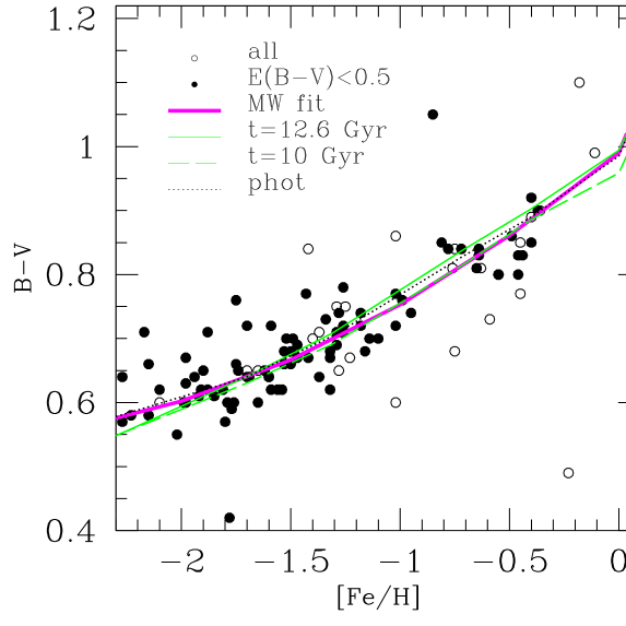
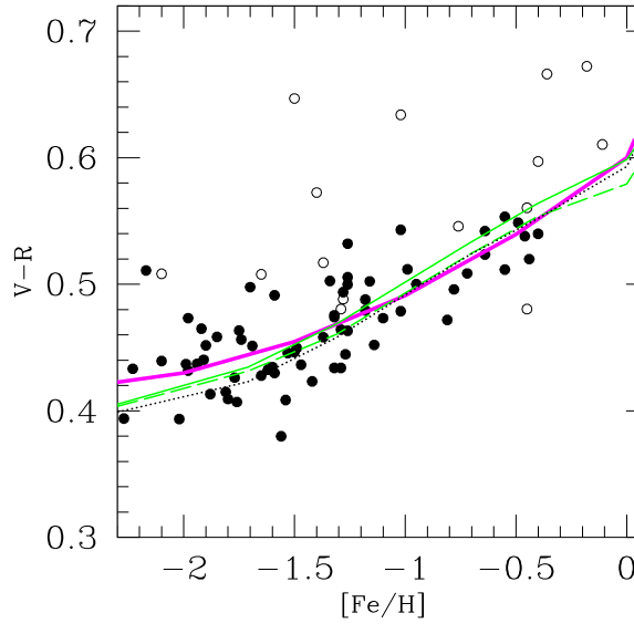
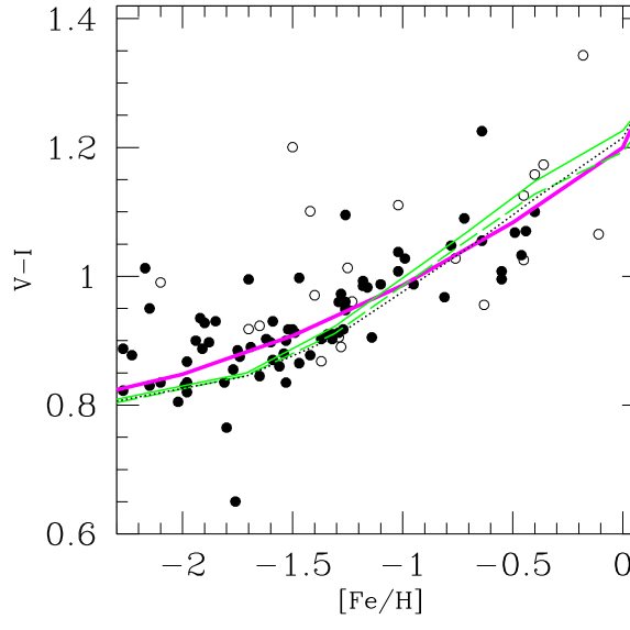
Figure 1: Optical colours in several bands as a function of metallicity for the MW globular clusters (Harris 1996 catalog; 2010 edition). Filled (open) circles represent globular clusters with reddening E(B$-$V)$\leq$0.5 ($>$0.5), de-reddened according to the extinction law of Cardelli, Clayton, & Mathis (1989). The magenta line shows a second order polynomial fit to the data with E(B$-$V)$\leq$0.5. The black dotted lines show the photometric predictions of the MILES models. The synthetic colours derived from the MIUSCAT SSP spectra for models with age of 12.6 and 10 Gyr, for different metallicities and Kroupa Universal IMF, are shown in solid and dashed green lines, respectively.

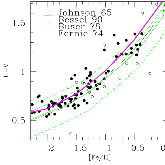
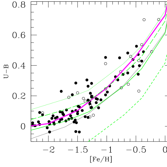
Figure 2: The same as figure 1 but for U$-$V and U$-$B colours. The green lines show the synthetic colours derived by using different definitions of the U filter: solid for the Buser & Kurucz (1978) filter, long-dashed for the Johnson (1965) filter, dotted for Bessel (1990) and short-dashed for Fernie (1974).

Here we use the catalogue of Harris 1996 (2010 edition) as a reference for the Milky Way (MW) globular clusters. The catalogue is a compilation of 150 clusters including the Johnson-Cousins UBVRI photometry, [Fe/H] metallicity and reddening E(B$-$V) among other data. Colours, except B$-$V, have been de-reddened using the extinction law of Cardelli, Clayton, & Mathis (1989).

Figure 1 shows the comparison of the optical broad-band colours of the GCs with the ones derived from the models. The model metallicity indicates the total abundance ratio [Z/H]. A fit to the data points with a second order polynomial is indicated to guide the eye. In order to avoid clusters with uncertain photometry due to high extinction, we excluded the most reddened clusters with E(B$-$V) $\geq$0.5 (open circles). The MIUSCAT models are shown for ages of 10.0 and 12.6 Gyr for a Kroupa Universal IMF. The use of a Salpeter IMF would leave the colours almost unaffected (with differences smaller than 0.01  mag). To derive the synthetic colours we adopt the Buser & Kurucz (1978) filter responses and Vega magnitudes. The zero point has been set by using the Hayes (1985) spectrum of Vega with a flux of $3.44\times 10^{-9}$ erg cm^-2 s^-1 Å^-1 at 5556 Å(see Falcon-Barroso et al. 2011 for further details on the computation of synthetic magnitudes). The colours of Vega in the Johnson-Cousins filters are assumed to be U$-$B=U$-$V=B$-$V=V$-$R=0 mag, V$-$I=-0.04 mag. The black dotted line represents the photometric SSP model predictions computed by adopting temperature-gravity-metallicity relations from extensive photometric stellar libraries (Vazdekis et al., 1996, 2010). The colour predictions resulting from these two approaches give very similar results (with differences of the order of 0.01-0.02 mag) showing the reliability of the flux-calibration of the model SEDs (see Paper I for more details).

Figure 1 also shows that the models reproduce the observed colours fairly well. Note that the V$-$I colour is particularly relevant to test the reliability of our models. This colour is heavily sensitive to the details of the method used to join the three libraries (MILES, Indo-U.S. and CaT). Indeed, the V magnitude is entirely measured within the MILES range, whereas the I filter response falls within the Indo-U.S./CaT range. The good match to the observed colours shows the robustness of the method and the flux-calibration of the MIUSCAT SEDs. It is also remarkable the ability of our models to reproduce the B$-$V colour. This has been for a long time a problem for stellar population synthesis models. As quoted in previous works (e.g. Worthey 1994; Maraston 2005), SSP model SEDs tend to provide systematically redder B$-$V colour than the observed values ($\approx$0.05 mag). One of the reasons of these discrepancies may be ascribed to difficulties of the theoretically-based models in modeling the spectral energy distribution around $\simeq$ 5000-6000  Å, where the theoretical spectra predict a flux excess. The use of empirical libraries (Pickles, 1998) has proven to be effective at improving the match with colours of luminous red galaxies (Maraston et al., 2009). Likely, the use of empirical libraries with good flux-calibration quality and good parameter coverage, including the metal-poor regime, has allowed us to improve the matching of the GC colours in comparison to previous works. The improved match of the B$-$V vs [Z/H] relation when using MILES-based models instead of the STELIB-Kurucz library has been also shown in Maraston et al. (2011).

In Figure 2 we show the results obtained for the U$-$V and U$-$B colours. We found that colours involving the U band are significantly more difficult to reproduce. Indeed, our models predict bluer colours ($\approx$0.1 mag in the high metallicity regime). As explained in Sect. 2.1, the U magnitude is not fully derived from the MIUSCAT SEDs, which do not extend to the blue end of the U filter response. The missing flux is accounted for with the aid of the (Pickles, 1998) stellar library. However we rule out this calibration as the a main source for the obtained discrepancy, as the obtained magnitudes following two different approaches (the second one employing SSP model SEDs from other authors) do agree within $\approx$0.02 mag. Moreover, even the photometric predictions show a similar level of disagreement with the data. A possible explanation may be linked to the various U filter response curves that can be adopted to reproduce the observations. Figure 2 shows the obtained results for various U filter responses, which differ from our reference filter (Buser & Kurucz 1978). Whereas for other Johnson broad-band filters the adoption of different references for a given filter usually implies minor changes, in the case of the U filter, the exact definition of the curve makes a significant impact on the obtained colours. For instance, if we use the Johnson (1965) response curve, we obtain a much better match. Since it is difficult to trace back the compilation of data to recover which filter has been used for every GC, the U$-$V and U$-$B colours are subject to this source of uncertainty.

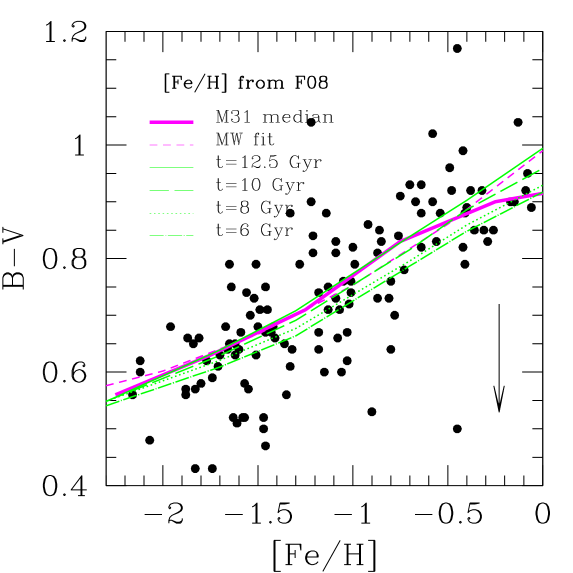
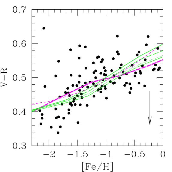
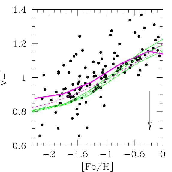
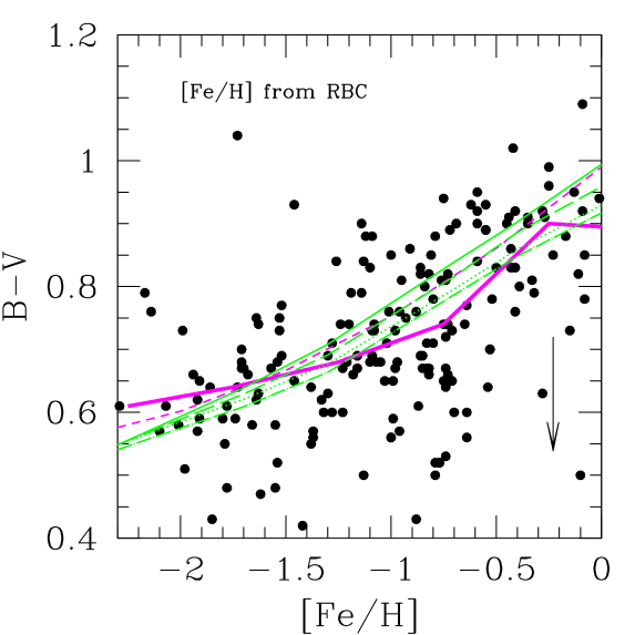
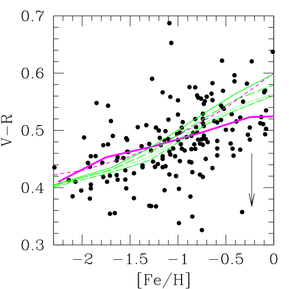
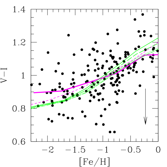
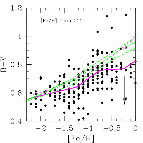
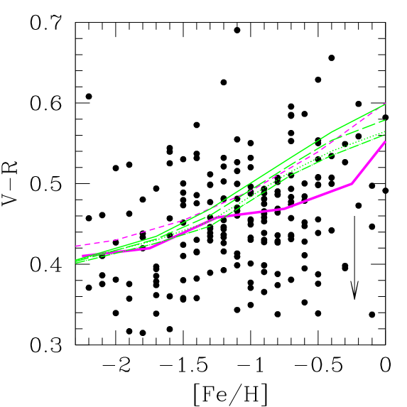
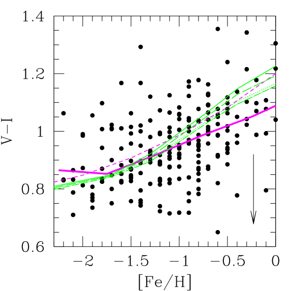
Figure 3: Optical Johnson-Cousins colours plotted against the metallicity for M31 globular clusters. In the first row of panels the metallicity and reddening measurements are taken from Fan et al. 2008, in the second row they come from the RBC, whereas in the last row we consider the catalog of Caldwell et al. (2011). Only clusters with reddening E(B$-$V)$\leq$0.5 are shown. The vertical arrow indicates the mean amount of de-reddening applied.The magenta thick solid line indicates the median to the data calculated in metallicity bins of $-2,-1.5,-1,-0.5,0$ and $0.5$ dex. The green lines are the synthetic colours derived from the MIUSCAT SSP SEDs for Kroupa Universal IMF and different ages: 12.6 (solid), 10 (dashed), 8 (dotted) and 6 Gyr (dashed-dotted).

4.2 M31 globular clusters

In this section we compare our models with the globular clusters of M31. For this purpose we use different photometric catalogs and metallicity estimates. We consider the spectroscopic metallicity determinations of Fan et al. (2008), which is a compilation of various sources (Huchra, Brodie, & Kent, 1991; Barmby et al., 2000; Perrett et al., 2002), the Revised Bologna Catalog (RBC), which are determined in a homogeneous manner (Galleti et al., 2009) and the spectroscopic catalog of Caldwell et al. (2011), hereafter C11. Integrated colours in the Johnson-Cousins system have been taken from the RBC, while photometry in the SDSS bands is from Peacock et al. (2010). The extinction in each band has been derived from the reddening values given in the corresponding catalog and the Cardelli, Clayton, & Mathis (1989) extinction law. Given the higher uncertainty in the M31 measurements compared to the MW GCs, we only consider clusters with low extinction values (E(B$-$V) $\leq$0.5) to avoid unreliable colour estimates. Only globular clusters classified as old in the catalogs are considered.

Figure 3 shows the Johnson-Cousins colours of the M31 GCs as a function of metallicity. Given the high dispersion of the points we found that the polynomial fit is not a good description of the data. To guide the eye, we overplotted the median of the colours computed in intervals of metallicity and compare it to the fit to the MW GCs. We also show the model lines corresponding to the SSPs with ages ranging from 6 to 12.6 Gyr (Kroupa Universal IMF). The Vega system used to compute the synthetic magnitudes is the same as adopted for the MW data. The SDSS colours in the AB system are shown in Figure 4. Note that the scatter obtained for the M31 data in these two figures is considerably larger than that observed in the MW clusters. Moreover, as shown by the arrows, the M31 clusters display a considerable amount of reddening.

Although the absolute colours of M31 can be subject to several uncertainties, a robust result inferred from Figures 3 is that the slope of the colour-metallicity relation is flatter in the M31 clusters. Given that the MW slope is consistent with that of the old models, we argue that in M31 a significant age variations with metallicity is needed to account for the different slope. A flatter relation than that indicated from the models is also seen in Figure 4 with SDSS colours. Old stellar populations in the lower metallicity regime and young ages for the metal rich clusters could explain such a trend. We obtain the worse fits to the data with the old models for the V$-$R and g$-$r colours. Indeed, the M31 GC colours are in general bluer than their Galactic counterparts, mainly in the high metallicity regime, as it can be inferred from comparing to the MW fit. The reason for this discrepancy at nearly solar metallicity may be linked to the fact that M31 clusters show higher metallicities than their MW counterparts (e.g., Beasley et al. 2005 ). In general the SDSS colours, even for intermediate metallicities, are matched better with younger models. However, it is worth noticing that the choice of the catalog may change our conclusion. In fact young models are required to fit the trend in the g$-$r colour of Fan et al. (2008) dataset, whereas models of 6-8 Gyr provide a fair match for all the colours of the RBC and C11 catalogs. From the comparison with our model lines the best match to the data is obtained combining old models at lower metallicities and younger models at the high metallicity regime.

In Peacock et al. (2011) the synthetic g$-$r colour derived from the models of Vazdekis et al. (2010) has been compared to the SDSS colours of M31 clusters in a similar way as it is done here. Since the g$-$r colour falls in the MILES range, it coincides with the predictions of the MIUSCAT models presented here. In Peacock et al. (2011) paper the Vazdekis et al. (2010) colours turned out to be offset by $\approx$0.1 mag at solar metallicity with respect to M31 GC colours. Although for the oldest model considered here we find similar difference in colour, by using different colours and different photometric systems we conclude that the data can be matched by considering younger models than those in Peacock et al. (2011). Finally, as we obtain with the old models very good fits to the MW clusters, which have more reliable data, and since the M31 cluster colours in the same photometric bands differ from the ones of the MW, we can conclude that we require younger models, at least in the high metallicity regime, to fit the data.

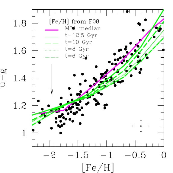
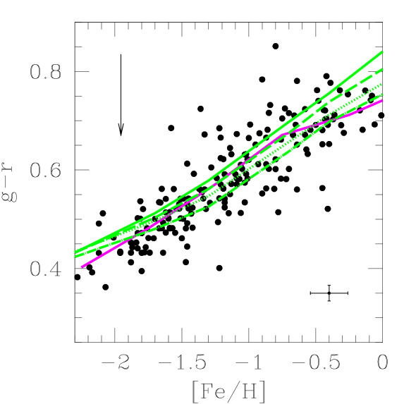
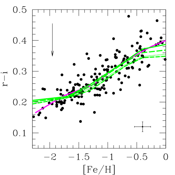
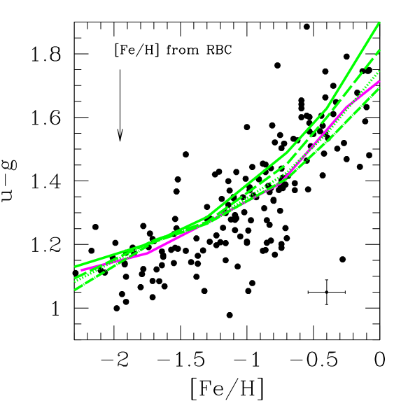
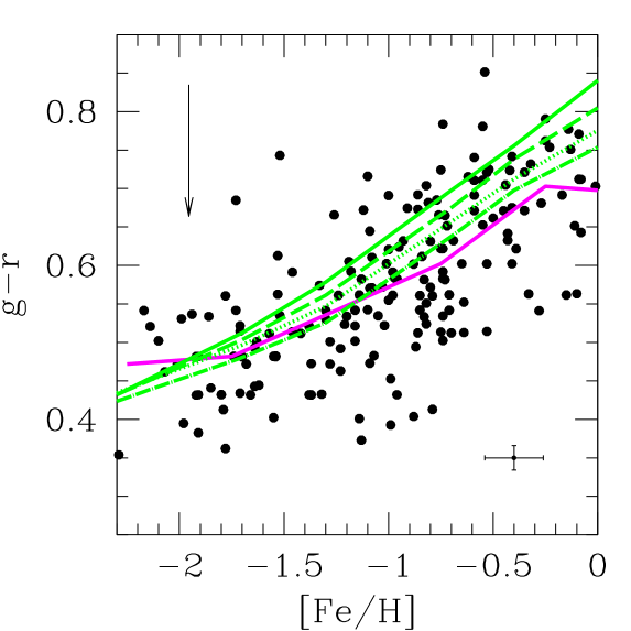
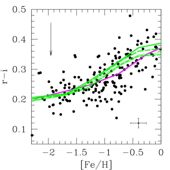
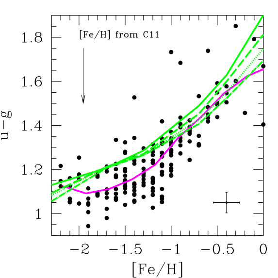
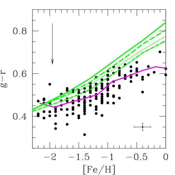
Figure 4: Same as in Figure 3 but for colours in the SDSS bands. The errorbars in the lower-right corner indicate typical errors on the metallicity and the photometric measurements.

Our results agree with evidences supporting that metal-rich GCs tend to be younger than the more metal-poor clusters, at least in the MW (e.g., Marín-Franch et al. 2009; De Angeli et al. 2005; Barmby & Huchra 2000; Rosenberg et al. 1999). Moreover, it has been claimed that the GCs of M31 tend to be on average younger than their Galactic counterparts (Beasley et al., 2005), though this result is yet to be conclusive. Spectroscopic ages for the high-metallicity M31 clusters have been derived in C11. In the low-metallicity regime the authors could not get accurate age determination, as these clusters are contaminated by blue HB stars, hence we can not test the age variation with metallicity. For the high-metallicity clusters in our sample ([Z/H]$\mathrel{\hbox{\hbox to0.0pt{\hbox{\lower 4.0pt\hbox{$\sim$}}\hss}\hbox{$>$}}}-1$) the C11 determinations give a mean age of 11.3 Gyr, that apparently contradicts the young nature of the M31 clusters. Note however that these authors employed the Balmer absorption line indices as age indicators and it is well known that this method can give very uncertain absolute ages, even larger than the age of the Universe (Vazdekis et al., 2001; Schiavon et al., 2002; Mendel, Proctor, & Forbes, 2007; Poole et al., 2010). Moreover, the models of Schiavon (2007) used in C11 give broad-band colours in excellent agreement with our values. For instance, a solar metallicity model with age of 11.2 Gyr has a B$-$V colours of 0.978 mag, very similar to B$-$V$=$0.977 mag that we obtain for the MILES models. Both photometric predictions are much larger than the M31 colours (Figure 3), confirming the discrepancy between the spectroscopic and photometric age measurements.

Furthermore, given the high uncertainties involved in the extinction, even our results should be taken with caution. Indeed, the parameter that varies mostly among the three catalogs is the reddening. The C11 estimates tend to be biased towards larger values than the other two catalogs, leading to bluer de-reddened clusters (see for instance the g$-$r colour in Figure 4). In C11 the quoted uncertainties for the $E(B-V)$ is 0.1 mag, hence of the order of colour variations due to different ages. Therefore, it is not possible to draw robust conclusions.

5 Colour evolution of Luminous Red Galaxies

In this section we consider the Luminous Red Galaxy (LRG) sample of Eisenstein et al. (2001), for which typically the definition of early-type galaxy (ETG) also applies. The LRG sample has been extracted from the SDSS spectroscopic galaxy survey (Data Release 7, Abazajian et al. 2009), by selecting galaxies with the GALAXY_RED flag in the SDSS database. LRGs constitute a uniform sample of objects with the reddest rest-frame colours, selected with cuts in the (g$-$r, r$-$i, r) colour-colour-magnitude cube (see Eisenstein et al. 2001). To obtain the same galaxy population at different redshifts, the LRG sample has been selected using two different selection criteria below and above z=0.4, as the Balmer break moves from the g band to the r band at this redshift. To increase the redshift range, galaxies from the 2df SDSS LRG and Quasar (2SLAQ) survey (Cannon et al., 2006) have been also included ($\approx$15000 objects) and they contribute to the high redshift tail of the redshift distribution (see Figure 5). By restricting the sample to galaxies with reliable redshift determination (zWarning$=$0) we end up with $\approx$170000 galaxies. The SDSS database provides a variety of measured magnitudes for each detected object. Throughout this paper, we use dereddened model magnitudes because they provide an unbiased colour estimate in the absence of colour gradients (Stoughton et al., 2002).

Figure 5: Redshift distribution for the LRG sample, which is composed of 168737 galaxies.

Previous works (Eisenstein et al., 2001; Wake et al., 2006) have highlighted the difficulties of stellar population models in reproducing the colour evolution in observed frame of LRG at intermediate redshift ($0.1<z<0.7$), with the prediction of too red colours in the g$-$r and too blue in the r$-$i for the lowest redshift LRGs, while the opposite effect is observed for the highest redshift LRGs. Similar disagreements have been reported for red sequence colours in galaxy clusters at similar redshifts (Wake et al., 2005).

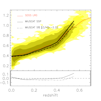
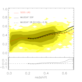
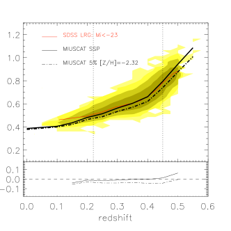
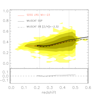
Figure 6: Colour evolution of the LRG sample in the r$-$i (left-hand panel) and i$-$z (right-hand panel) bands. The contours enclose 20%, 40%, 60% and 95% of the galaxies. The red thin line shows the median colour at different redshift bins equally spaced in intervals of 0.025. The black thick line shows a passive evolution model with solar metallicity and redshift of formation of 5 (corresponding to an age of 12.6 Gyr at z$=$0) for a Kroupa Universal IMF. The dot-dashed line indicates a model that includes a 5% contribution in mass from a metal-poor ([Z/H]=-2.32) stellar population. The residuals between the synthetic and observed colours are shown in the bottom panels using the same scale. The bottom panels show the colour evolution for a subsample of LRGs having absolute magnitude: $M_{i}<$ -23 mag. The dotted vertical lines indicate the redshift range where these bright galaxies are a coeval population according to Tojeiro & Percival (2011b).

In Figure 6 we compare the predictions from the MIUSCAT models to the colour evolution of the LRG sample. According to the fiducial model for the formation of LRG, in the simplest case we assume that they formed in a uniform burst at high redshift (z$=$5) and evolve passively thereon. Solar metallicity and Kroupa Universal IMF are assumed. The observed colours are reproduced by shifting the model spectra to the corresponding redshift and taking into account the ageing effect. Synthetic colours in the SDSS filters have been computed in the AB system (Oke & Gunn, 1983). For consistency, the observed colours from the SDSS database have been transformed to AB system by applying the relative shifts: $u_{AB}=u_{SDSS}-0.04$ mag; $z_{AB}=z_{SDSS}+0.02$ mag. The model predictions are shown for the redshift interval where the MIUSCAT spectra cover the r$-$i and i$-$z colours. The g filter falls outside the measurable range at z$=$0.05, thus colours containing u and g are not shown. We see that the simplest model is able to reproduce the observed distribution at low redshift in both colours. The model starts to deviate from the median colours at z$\sim$0.4, producing too red colours.

In Figure 6 it is represented also a second model, where a small fraction of the mass (5%) is contributed by a metal-poor population ([Z/H]$=$-2.32). It is expected (Worthey et al., 2005; Pagel, 1997) that galaxies exhibit some spread in the metallicity distribution with a contribution also from metal-poor stars. The effect of including stars with such a low metallicity is to bluen the colours, with the result of loosing the match with the observed distribution in the lowest redshift range, but improving it at high redshift. It is worth to say that the differences between this model and the median of observed colour is only $\approx$ 0.02 mag. The uncertainties derived from the zero-point calibration of the SDSS system (0.01 mag) and from the choice of the IMF (0.01 mag of difference between Salpeter and Kroupa Universal) could also account for this difference. Hence, it turns out to be difficult to discriminate among these two possibilities. Nevertheless, in both cases the MIUSCAT models perform rather well, confirming the results of Maraston et al. (2009), according to which models constructed with empirical stellar libraries provide a good fit to the LRG colour distribution.

Although the LRG sample has been selected to follow a passive evolution model (see Eisenstein et al. 2001), this does not guarantee that all the galaxies accomplishing the selection criteria follow this model. In Tojeiro et al. (2011a) it has been shown that a non negligible fraction of LRGs does not evolve passively in a dynamical sense. They can undergo mergers and the sample can be contaminated with galaxies that belong to the LRG sample for a short period of time. However, the brightest tail of the sample turns out to be coeval (i.e. with almost no merging) for galaxies in the redshift range: 0.22-0.45. For this reason, in the bottom panels of Figure 6 we compare our passive evolution models with these bright galaxies ($M_{i}<$ -23 mag). For this subsample, the high-redshift galaxies are truly the progenitors of the low-redshift ones. In the redshift range where the galaxies appear coeval, our passive model performs remarkably well.

6 Nearby Early-Type Galaxies

Figure 7: Redshift distribution for the ETG sample of Nair & Abraham (2010). The red lines indicates our sample at z$\simeq$0.04, which includes 370 objects.

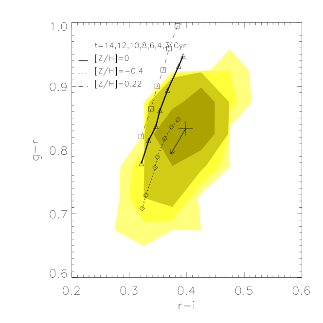
Figure 8: Observed colour distributions in the SDSS bands for the ETG sample at z$\simeq$0.04. The contours enclose 20%, 40%, 60% and 95% of the galaxies and the cross indicates the median colours ($u-g=1.83$, $g-r=0.83$, $r-i=0.40$ mag). The arrow indicates the colour de-reddening when an internal extinction of $A_{V}=0.2$ mag is assumed. Synthetic colours derived from the MIUSCAT SEDs for a Kroupa Universal IMF are overplotted. The different lines join models with the same metallicities for ages ranging from 3 to 14 Gyr.

A further insight into the capabilities of the models can be obtained by comparing them to a sample of nearby galaxies, for which we can use three different colours as constraints. For this purpose we select a homogeneous sample in the Local Universe with a large number of SDSS galaxies with visual morphological classification (Nair & Abraham, 2010). We select a subsample of early-type galaxies (morphological type $T\leq-4$) with reliable redshift measurements. We further restrict our sample to a narrow redshift slice, $0.035<z<0.045$, to end up with 370 targets. This choice of redshift is motivated by two main reasons. First, at this redshift the number of galaxies peaks (see Figure 7). Second, given the limited spectral coverage of the MIUSCAT models in the blue end, the correction factors we need to apply to measure the SDSS u magnitude become too large for redshifts above this value, as the wavelengths at which the u filter response peaks start to fall outside the spectral range of the models (see Paper I). Before comparing the colours derived from the MIUSCAT SEDs, once redshifted to z$=$0.04, we have tested that the selected redshift interval is small enough that colour differences due only to variation in redshift within such interval are negligible ($<$0.01 mag).

As for the photometric estimates, we rely on the model magnitudes from the DR7 catalog. It is worth noticing that all the colours involved in this study belong to the optical spectral range, which are known to be heavily affected by the age/metallicity degeneracy, irrespective of the colour-colour diagnostic diagram in use. Therefore the results obtained in this section are not intended to provide a well-constrained picture for the stellar populations of these galaxies, which might require a deeper analysis involving colours in other wavelengths and/or spectra.

In Figure 8 we show the colour distribution of the ETG sample compared to the MIUSCAT SSP models with ages ranging from 3 to 14 Gyr for three metallicity values: [Z/H]$=$-0.4, 0 and 0.22. We also include an arrow indicating the effect of internal dust extinction on the observed colours. We assume $A_{V}=0.2$ mag, in agreement with the typical value derived for low redshift LRG (Tojeiro et al., 2011a). The de-reddening in the various SDSS bands has been computed with the extinction law: $\tau_{\lambda}=\tau_{V}(\lambda/5500\AA)^{-0.7}$ (Charlot & Fall, 2000). We see that none of the SSP models is able to match the observed colour distribution. Although the fiducial model for the formation of ETGs predicts that they form in a uniform burst at high redshift with high metallicity, the old models tend to produce too red colours in the g$-$r vs u$-$g plot. On the contrary, the r$-$i colours turn out to be too blue with respect to the real galaxies. Hence, this simple picture does not seems to appropriate to describe the stellar populations of this galaxy sample.

The MIUSCAT models adopt the stellar isochrones of Girardi et al. (2000) (i.e. Padova 2000), as described in Paper I. It has been claimed that these tracks provide blue colours for old elliptical galaxies. Bruzual & Charlot (2003) claimed that models computed with the isochrones of Bertelli et al. (1994) (i.e. Padova 1994) are preferred because redder V-K colours are predicted, in better agreement with the observations. For the optical spectral range the net effect of adopting these two sets of stellar tracks is almost negligible. Using the Padova 1994 tracks, Bruzual & Charlot (2003) obtained redder colours than using Padova 2000: u$-$g by $\approx$0.02 mag and g$-$r and r$-$i by $\approx$0.01 mag. Therefore these results tend to worsen the obtained mismatch for the bluer colours.

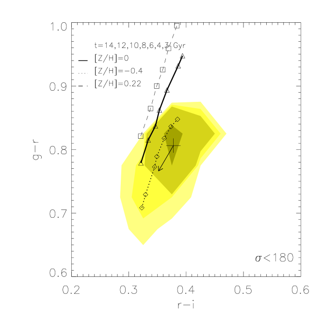
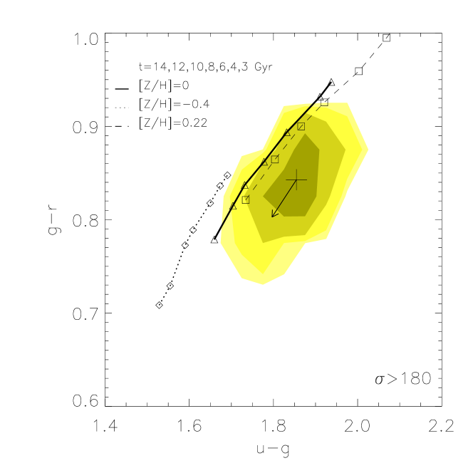
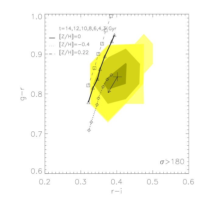
Figure 9: Upper panels: observed colour distribution for ETGs with velocity dispersion below 180 km s^-1, compared to the same SSP models as in Figure 8. Bottom panels: colour distribution for ETGs with velocity dispersion above 180 km s^-1. The median colors of the observed distribution for low and high velocity dispersion objects are, respectively: $u-g=1.76$, $g-r=0.81$, $r-i=0.38$ mag and $u-g=1.87$, $g-r=0.85$, $r-i=0.40$ mag.

To understand better the origin of this mismatch and to avoid possible sample selection biases we have divided the ETG sample in intervals according to their masses. In Figure 9 we show the colour distributions corresponding to galaxies with velocity dispersions above and below 180 km s^-1. This value allows us to separate galaxies with different properties, while keeping almost equally populated these two galaxy mass ranges. ETGs with high velocity dispersion are generally found to exhibit older ages and higher metallicities than their low velocity dispersion counterparts (Trager et al., 2000; Sánchez-Blázquez et al., 2006), resulting in redder colours. We see that none of the SSP models plotted in this Figure is able to match the distribution of massive ETGs. Galaxies with lower velocity dispersion tend to be matched with models of lower metallicity and age $\simeq$8 Gyr, even though the predicted u$-$g remain too blue ($\simeq$0.1 mag). Although a better agreement is obtained, the models do not provide fully satisfactory fits.

The colour predictions computed by adopting SSP models from different authors are shown in Figure 10. We considered the BC03 and Maraston (2005) models, the two based on the BaSeL theoretical stellar library (Lejeune, Cuisinier, & Buser, 1998) and the Maraston et al. (2009) models that use the Pickles (1998) empirical library. The BC03, Maraston (2005) and Maraston et al. (2009) adopt a Salpeter IMF, whereas the MIUSCAT models are shown for both Salpeter and Kroupa IMF, showing that the choice among these commonly used IMFs has little effect on these colours. Although none of the models can fairly reproduce the observed distribution, it is remarkable the advantage of using models based on empirical-based libraries. These models predict g$-$r bluer by 0.06 mag and r$-$i redder by 0.05 mag compared to the models based on theoretical libraries. The Maraston et al. (2009) models predict slightly bluer g$-$r and redder r$-$i colours than the MIUSCAT SEDs by $\approx$0.01 mag, but also redder u$-$g colour.

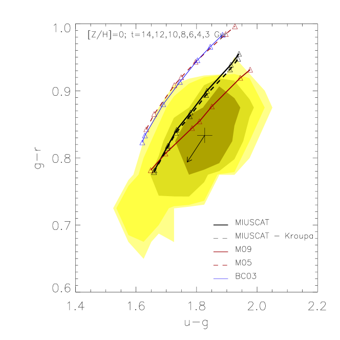
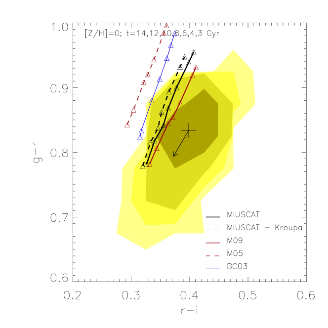
Figure 10: Same as in figure 8 for stellar populations models from different authors. For this comparison only models for solar metallicity are shown. The blue line corresponds to the BC03 models assuming a Salpeter IMF. Red dashed line represents the M05 models based on theoretical stellar atmospheres, whereas the solid red line shows the models from the same authors based on the Pickles empirical stellar library (Maraston et al., 2009). In these two cases a Salpeter IMF is adopted by these authors. Finally the black lines indicate the MIUSCAT model tracks adopting the Salpeter (solid line) and Kroupa Universal (dashed line) IMF.

6.1 IMF effects

Here we explore how these colours vary when adopting different IMF shapes and slopes. We consider the power-law unimodal IMF defined in Vazdekis et al. (1996) for different slopes for the solar metallicity SSP models with the same ages considered in Figure 8. Figure 11 shows a very modest variation of the bluer bands. However varying the IMF turns out to have a significant effect on the r$-$i colour. Indeed, by assuming a very steep IMF slope ($\mu=2.3$) the colour distribution in the g$-$r vs r$-$i diagram can be matched, though for relatively young ages (3-4 Gyr). On the other hand the g$-$r vs u$-$g colour distribution is not reproduced for none of the represented models.

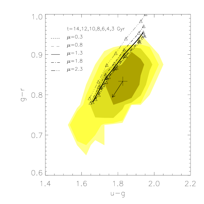
Figure 11: Same as in Figure 8 for unimodal IMF with different slopes.

6.2 Two-burst model: inclusion of a metal-poor component

We relax here the assumption that ETGs are SSPs and use stellar populations with two main bursts to model these galaxies. The first model tested is the same used for the description of the LRG colour evolution shown in Section 5. We include a small contribution of 5% to the total mass, with a primordial chemical composition ([Z/H]=-2.32) and very old age (14 Gyr). This should resemble the first population of stars formed before being enriched by the subsequent star formation. As shown also by Maraston et al. (2009), the contribution of metal-poor stars is effective in bluening the g$-$r, without perturbing too much the r$-$i colour. The resulting MIUSCAT two-burst colours are shown in Figure 12. As expected, all the colours become bluer, improving the match with the observed colour-colour distribution in the g$-$r vs u$-$g diagram. The resulting r$-$i colour becomes slightly bluer, but since the effect of the metal-poor component is stronger on the bluer bands the colour distribution in g$-$r vs r$-$i improves as well, in agreement with the finding of Maraston et al. (2009). However the inclusion of such metal-poor component alone is not sufficient to fairly reproduce the observed colour-colour distributions.

6.3 Two-burst model: inclusion of a young stellar population

A similar effect is seen when a young component is included. In Figure 13 the plotted model includes a small contribution (3% of the total mass) of a young stellar population of 1 Gyr. In this case the effects on all the colours is more pronounced than in Section 6.2. This model can successfully explain the colour-colour distribution in the g$-$r vs u$-$g diagram, but not the r$-$i colour, since the predicted values are far too blue ($\approx$0.06 mag). Therefore, these models are not able to match the two colour-colour diagrams simultaneously.

Figure 12: Same as in Figure 8 but for a two-burst model that includes a metal-poor population ([Z/H]=-2.32) of 14 Gyr, which contributes with a 5% to the total mass.

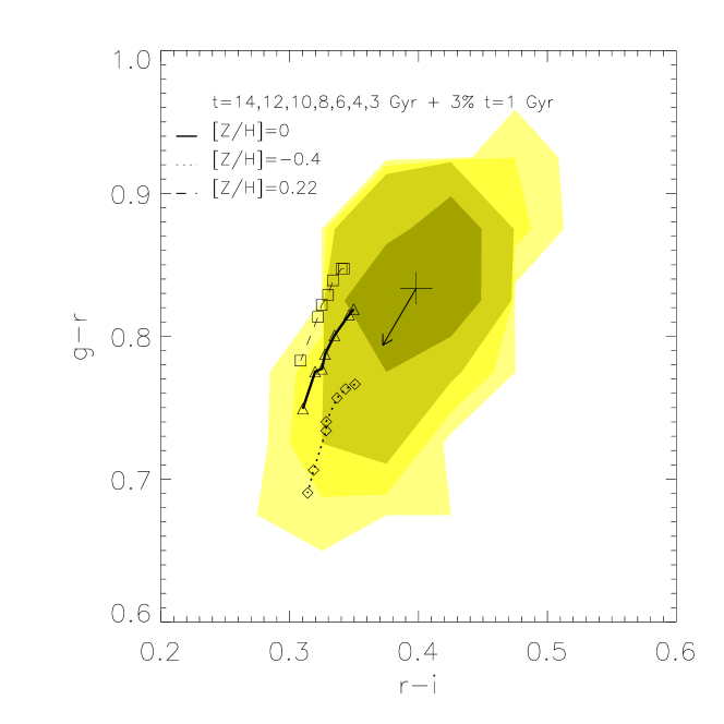
Figure 13: Same as in Figure 12 for a two-burst model including a 3% contribution in mass from a 1 Gyr stellar population.

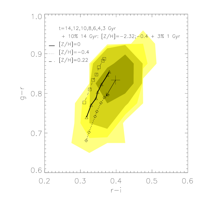
Figure 14: Same as in Figure 8 but for the SFH derived from the chemo-evolutionary model described in Vazdekis et al (1996, 1997). We model it by adding on the top of the main episode of star formation the contributions of two stellar populations: 10 % of the mass formed at 14 Gyr with a top-heavy IMF (slope $\mu$=0.8). Half of the mass formed in this burst is in metal-poor component ([Z/H]=-2.32 dex) and half of it has subsolar composition, [Z/H]=-0.4 dex. Finally, there is a 3% contribution to the total mass from a component of 1 Gyr. The stars formed in the main episode and afterwards are skewed towards lower masses according to a steeper IMF slope ($\mu$=2.3). We use here the Bimodal IMF defined in Vazdekis et al. (1996).

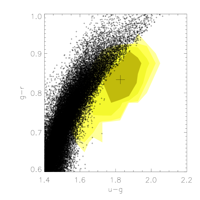
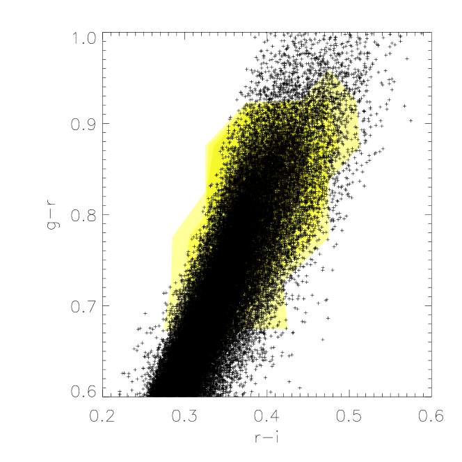
Figure 15: The observed colour-colour distributions are compared with simulated points derived from the three-bursts Montecarlo SFHs described in Section 6.5.

6.4 Three-burst model: chemo-evolutionary model with varying IMF slope

Here we switch for the first time to the combination of more than two stellar populations. In Sections 6.2 and  6.3 we have seen that the combination of an old metal-rich stellar population with a small fraction of either a metal-poor or a young component has significant effects on the resulting colour-colour plots. Furthermore in Section 6.1 we tested the effects on the colours from non standard IMFs. In fact, very recently van Dokkum & Conroy (2010) showed spectroscopic evidences pointing towards steeper IMFs in massive galaxies, in agreement with previous studies (e.g., Faber & French 1980; Carter, Visvanathan & Pickles 1986; Vazdekis et al. 1996; Cenarro et al. 2003). Therefore it is worth to test the colours that result from combining all these stellar populations. An example of such scenario is the one derived in Vazdekis et al. (1997) from the best fits to both broad-band colours (from $U$ to $K$) and the Lick line-strength indices, of a number of prototype massive galaxies, employing a full chemo-evolutionary version of our models (Vazdekis et al., 1996).

In this scenario the IMF varies with time, being skewed towards high-mass stars during an initial short period of time ($<$0.5 Gyr) that quickly enriches the interstellar medium and, afterwards, the IMF becomes even steeper than the Salpeter one. This is reproduced with a multiple bursts model by adding on top of the main episode of star formation, that forms 87% of the mass, two populations. In the first population 10 % of the mass formed at 14 Gyr with a top-heavy IMF (slope $\mu$=0.8). Half of the mass formed in this burst is associated with a metal-poor component, [Z/H]=-2.32 dex (as in Section 6.2), and the other half has subsolar composition ([Z/H]=-0.4). Another 3% of the mass is formed at the age of 1 Gyr (as in 6.3). The stars formed in the main episode and at late times are skewed towards low-mass ($\mu$=2.3) (as in Section 6.1). A bimodal IMF is assumed for all these models. The adoption of the IMF with slope 2.3 in the main burst is consistent with recent evidences for a steep IMF in massive galaxies (van Dokkum & Conroy, 2010).

Figure 16: Mean IMF slope versus mean metallicity for the best solution SFHs from the Montecarlo simulations described in Section 6.5. The solid black line shows the relation found in Cenarro et al. (2003), whereas the dotted line is the linear fit to the points, obtained with a least squares fit in the X direction.

This model is shown in Fig. 14. For solar metallicity it is quite successful at matching the bulk of the galaxy distribution, although some problems persist in the r$-$i colour, which remains too blue. Although quite unlikely, part of this discrepancy can also be attributed to internal extinction, leading too red colours that we cannot fit with dust-free models.

6.5 Three-burst models: Montecarlo simulations

In order to explore all the possible combinations of SFHs that can match the two colour-colour distributions we have run a set of Montecarlo simulations, where we allow all the stellar population parameters to vary: age, metallicity and IMF slope. We only consider seven representative IMF slopes: 0.3, 0.8, 1.3, 1.8, 2.3, 2.8 and 3.3. To keep the case as general as possible we use three bursts, where the fraction of mass involved in each of the burst is also a free parameter. Figure 15 shows the results for 100000 simulations. On one hand we see that the cloud of models does not properly match the observed galaxy distribution in the g$-$r vs u$-$g plot. On the other hand, the cloud of models matches the region enclosed by data in the g$-$r vs r$-$i plot.

To understand which kind of SSP mixtures most likely resemble the data we selected the closest 1700 points to the median of the observed colours in each of the distributions. Among these combinations we only choose those that are common to these two distributions to end up with 26 models, whose SFHs are shown in the Appendix. We have ordered all these models following an increasing contribution of young stellar populations, i.e., with ages smaller than 5 Gyr. We see that a large number of models require very important contributions from SSPs with old ages, high metallicity (solar or higher) and IMF slopes steeper than Salpeter (i.e. $\mu>1.3$). All these models require smaller, but not negligible, contributions from young or/and metal-poor stellar populations. Finally SSPs with slopes lower than the Salpeter value seem to be required for a number of models. A mean solution for these models can therefore be summarized as mainly composed of metal-rich and dwarf-dominated stellar populations with much smaller contributions from young or metal-poor components. Interestingly the scenario discussed in Section 6.4 would be a good representative of this mean trend of solutions. In fact we nearly recover it in the models shown in the first and second rows of panels of Figure 18. Whereas many studies support the presence of old ages and metal-rich stellar populations in massive galaxies (see for example the review of Renzini 2006), the requirement of non standard IMFs is a matter of debate as recently pointed out by van Dokkum & Conroy (2010). Among our solutions, the steeper IMF slopes are recovered for the highest metallicity objects. In Figure 16 we show the mass weighted mean IMF slope as a function of the mass weighted mean metallicity for the 26 solutions. The existence of a IMF slope - metallicity relation has already pointed out by Cenarro et al. (2003). Interestingly, the linear fit to the simulated points lies close to the relation derived by the above authors by means of near-IR IMF sensitive spectral features. It is worth to note that, using completely independent diagnostic techniques, it is inferred a similar IMF-metallicity relationship in the sense that larger metallicities correspond to larger effective IMF slopes.

There are a number of models that depart significantly from the mean trend depicted above (see last rows of Figure 18). These models require important contributions from stellar populations with ages smaller than $\sim$5 Gyr. However we also see that most of these models also require steeper IMF slopes than the models that are clearly dominated by old stellar populations. This can be explained by the fact that the colours redden with increasing age, metallicity or IMF slope as shown in Paper I. Such degeneracy between these three parameters for the optical colours does not allow us to provide a unique solution. To constrain the solutions it is required to use spectroscopic data or/and colours in other spectral ranges (e.g., Vazdekis et al. 1997).

However it is worth recalling that none of the SFHs explored in the simulations provide satisfactory fits to these two observed colour-colour distributions. Indeed, the departure of the models from the median of the observed colours is non negligible, with the $u-g$ colour showing the largest residuals. It is beyond the scope of this paper to recover the SFHs of the SDSS early-type galaxy sample, but the fact that in these complex models we allow to vary all, the age, metallicity and IMF slope of the SSPs, without reaching a fully satisfactory solution, supports the need for a fourth parameter to be taken into account in the models. We consider such a possibility in the next section.

6.6 Effect of $\alpha$-enhancement

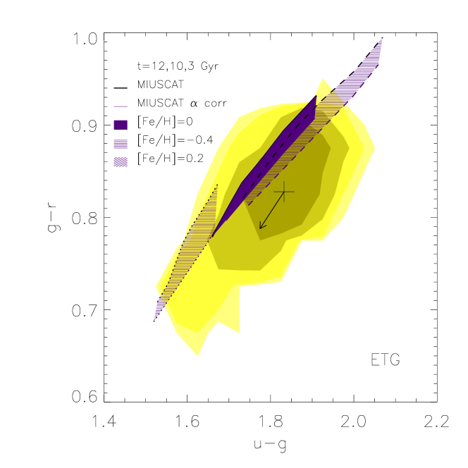
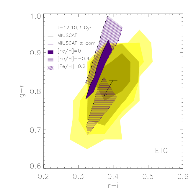
Figure 17: The observed colour-colour distributions are compared to the MIUSCAT SSP models once corrected from the $\alpha$-enhancement effect. There are three shaded regions corresponding to each metallicity. For each of these regions the upper envelope indicates the MIUSCAT SSP models (same as in Figure 8), whereas the lower envelope shows the resulting models once corrected from the $\alpha$-enhancement effects with the aid of the models of Coelho et al. (2007). For this purpose we estimate the colour difference obtained from comparing the scaled-solar and $\alpha$-enhanced ([$\alpha$/Fe]=0.4 dex) models from these authors.

As explained in Paper I the MIUSCAT SSP SEDs employed here are computed on the basis of scaled-solar isochrones and stellar spectra with nearly scaled-solar abundance ratios for the high metallicity regime that is required to fit massive galaxies. However, it is well known that the spectra of these galaxies show an enhancement in [Mg/Fe]. To assess the effects of $\alpha$-enhanced element partitions on the SSP colours we correct them, in a differential way, with the aid of the models of Coelho et al. (2007). These fully theoretical models are constructed on the basis of a high resolution library of synthetic spectra (Coelho et al., 2005), where all the $\alpha$ elements, including magnesium, are enhanced with respect to iron with the same proportion, i.e., [$\alpha$/Fe]=0.4.

We correct our MIUSCAT SSP colours with the difference in colour obtained from the scaled-solar and $\alpha$-enhanced models of Coelho et al. (2007), keeping constant the iron abundance. The corrected SSP colours are shown for different metallicities in Figure 17. Interestingly, the effect of $\alpha$-enhancement tends to bluen the u$-$g and g$-$r colours and to redden r$-$i, as required by the data. Note that although this effect is relatively modest it certainly goes in the right direction for improving our fits to the most massive galaxies of our sample. Preliminary tests performed with our own version of the models constructed with $\alpha$-enhanced mixtures based on the MILES library, making use of the [Mg/Fe] determinations of Milone, Sansom, & Sánchez-Blázquez (2011), lead to even larger differences with respect to the scaled-solar predictions in the same directions as with the models of Coelho et al. (2007).

7 DISCUSSION AND CONCLUSIONS

In the present work we have explored the constraints on the MIUSCAT models provided by photometric data of globular clusters and quiescent galaxies. In Paper I we have presented the new models and described the improvements. Here, we have focused on the comparison of the model predictions with broad-band photometry.

The integrated colours of MW globular clusters can be remarkably reproduced by the MIUSCAT models in all the visible bands. Only colours involving the U filter can not be used to constrain the models, as the uncertainty relative to the filter response used to reproduce the U magnitude is too high. The ability of our models for matching the colours of the MW stellar clusters in the other bands is remarkable. In particular, the B$-$V colour has always challenged models based on theoretical stellar libraries, which fail at matching the range covered by the $V$ filter. Here we have shown that the problem can be solved by the use of empirical stellar libraries (see also Maraston et al. 2011).

The comparison with M31 globular clusters is less straightforward but it allows us to test the models even in the region of solar metallicity. The comparison with our models suggests that the M31 globular clusters are on average younger than usually assumed for the MW globular clusters. Although an old model (12.6 Gyr) can fit the metal-poor clusters, we need ages in the range 6-10 Gyr to match the colours of the clusters with high metallicities.

The spectral coverage of the MIUSCAT library allows us to test here the models in several bands and, by relaxing the assumption that all the M31 GC are old, we can obtain a good fit to the data if we assume that metal-rich M31 clusters are younger than metal-poor ones. The fact that in MW clusters we do not need young models may be ascribed to the lack of metal-rich clusters. Therefore our results disagree with previous works (Peacock et al., 2011) claiming that the g$-$r colours of M31 globular clusters could not be matched accurately with our models. Nevertheless, the large amount of extinction in these clusters makes their colours very uncertain and not suitable for calibration purposes.

When the models are compared to the colour evolution of LRGs, under the assumption of a passive evolution model, the observed colours are fairly reproduced. Both, a simple model where stars formed in a single burst at high redshift, and a model that includes a small component of metal-poor stars, can be used to fit the observed distribution with increasing redshift. However, in the high redshift interval (z $\mathrel{\hbox{\hbox to0.0pt{\hbox{\lower 4.0pt\hbox{$\sim$}}\hss}\hbox{$>$}}}$ 0.4) where the observed colours probe the rest-frame g$-$r, the models predict redder colours than the median distribution.

Although the colour evolution of the LRGs can be fairly described within the fiducial model of purely passive stellar evolution, the combination of three colours, u$-$g, g$-$r, r$-$i, poses a challenge. We find that the colour-colour diagrams based on these colours allow us to discriminate among different models. Given the wavelength coverage of the MIUSCAT models, we restrict our study to a limited redshift range, at z$\simeq$0.04, where we can measure all these three colours. Our study shows that single-burst models do not provide a good description for the local population of quiescent galaxies. Irrespective of their metallicity, the old SSPs provide too red u$-$g and g$-$r colours and too blue r$-$i colour. We also find that the SSP model predictions from different authors do not match these colour-colour distributions. Such disagreement has also been shown by Conroy & Gunn (2010). We note that the use of only two colours, u$-$g and g$-$r does not allow to highlight the problem in the r$-$i colour, which goes in the opposite direction. Nonetheless, an important result drawn from such a comparison is that models based on empirical stellar libraries (MIUSCAT; Maraston et al. 2009) predict colours much closer to the observed distribution than models based on theoretical spectra (Bruzual & Charlot, 2003; Maraston, 2005).

We rule out that the inability of the MIUSCAT SSP models for providing fully satisfactory fits to the colours of LRGs is due to flux-calibration issues. As shown in Paper I, the MIUSCAT spectra provide colours with photometric uncertainties $\mathrel{\hbox{\hbox to0.0pt{\hbox{\lower 4.0pt\hbox{$\sim$}}\hss}\hbox{$<$}}}$ 0.02 mag. Furthermore, the colours of our models are in good agreement with globular cluster data.

We have tested the hypothesis that quiescent galaxies formed their stars in a strong burst at high redshift. Our study based on the u$-$g vs. g$-$r and r$-$i vs. g$-$r colour-colour diagrams suggest that the constituent stellar populations of local ETGs are not necessarily fully coeval and old, and might require small contributions from either young or/and metal-poor stellar populations. We have explored several models with such complex stellar populations. We find that these smaller contributions are very effective at bluening the colours and matching the distribution in the u$-$g and g$-$r colours. Note however that the resulting r$-$i colour is too blue.

The chemo-evolutionary model shown in Vazdekis et al. (1996) provides one of the best fits to these two colour-colour diagrams. Apart from the inclusion of a metal-poor population at early-times and a small burst at 1 Gyr, this model adopts a variable IMF scenario. In this model the first generation of stars is skewed toward high-mass (top-heavy IMF), while at later times stars formed with a steeper IMF slope. The adoption of such a steep IMF is the main reason for the improvement also in the r$-$i colour. Although this model is just one among several possible solutions, it clearly shows the need for a more complex SFH than the single burst model to explain the formation of ETGs. Moreover, the finding that quiescent galaxies have experienced a small amount of recent star formation is not new and has been revealed by several observational evidences (Trager et al., 2000; Bressan et al., 2006; Kaviraj et al., 2007; Sarzi et al., 2008; Tojeiro et al., 2011a) and predicted by hierarchical models of galaxy formation (De Lucia et al., 2006; Ricciardelli & Franceschini, 2010). However, it is worth noting that although the colours obtained from these complex models are approaching the observed values, the agreement is not satisfactory.

An experiment done by simulating three-burst Montecarlo SFHs confirmed the impossibility of the three model parameters (age, metallicity and IMF slope) to fairly match the color plane g$-$r vs u$-$g. We are aware of the degeneracies affecting the optical colours, which do not allow us to properly constrain the solutions. It is beyond the scope of this work to fully constrain the SFHs, for which spectroscopic data or colors in other spectral range would be required, but the inability of these simulations to reproduce the observed colours suggests the need of another parameter to model the observations. We have identified that the inclusion of $\alpha$-enhancement improves the fits. A limitation of the models based on empirical libraries is that they rely on stars from the solar neighborhood, which, most likely, has experienced a chemical enrichment that differs from that of massive elliptical galaxies. Indeed, it is now well established that massive early-type galaxies are enhanced in Magnesium with respect to Iron, showing $[Mg/Fe]\simeq 0.2$ (Worthey, Faber, & Gonzalez, 1992; Trager et al., 2000; Yamada et al., 2006). We have estimated the effect of $\alpha$-enhanced models on these colours by applying differential corrections derived from the models of Coelho et al. (2007) predictions on the MIUSCAT colours. The overall effect is in the direction of improving the fits to the observations, as the colours in the bluer bands become bluer whereas the r$-$i tends to redden. Therefore, the combination of both effects, a more complex SFH and the inclusion in the models of abundance ratios in agreement with the observations should provide better fits.

We conclude that the impact of $\alpha$-enhancement on the colours of massive galaxies can not be neglected to properly reproduce the observations. Our forthcoming models taking into account the $\alpha$-enhanced mixture of MILES stars will clarify this issue.

Appendix A Results from Montecarlo simulations

In this section we show the SFHs of the best solutions found in the Montecarlo simulations described in Section 6.5. We selected the 1700 closest points to the median of the observed colours in each of the colour-colour plots. Then we only considered the solutions that satisfy both distributions, ending up with 26 models, whose SFHs are shown in Figure 18. The SFHs are ordered according to an increasing fraction of mass in bursts younger than 5 Gyr (the first panels show the solutions with the smaller fractions).

The resulting SFHs can be divided into two broad categories. In the first group we can identify SFHs dominated by an old, metal-rich population, enriched with dwarf stars (high IMF slopes). On top of the old populations, we find small contributions from young populations. In some cases we do not see any significant young component. In these cases, blue g$-$r and u$-$g colours result from the contribution of a metal-poor population (see also section 6.2).

The other group of solutions includes SFHs with an important component of young populations ($\leq$ 5  Gyr). In some cases, the fraction of mass formed in the youngest burst can be as large as 80% (see SFH in the last row). As already shown in Section 6.3, the age is the dominant parameter at decreasing both the g$-$r and u$-$g colours and, thus, it provides a good match of the g$-$r vs u$-$g plot. The SFHs with the largest component of young stellar populations also show the steepest IMF slopes, which are needed in order to redden the r$-$i colour. This confirms the results found in sections 6.1, 6.2 and 6.3, where we have illustrated how the IMF is mainly affecting the r$-$i while age and metallicity variations are needed to match the g$-$r vs u$-$g colour distribution.

Given the age/metallicity/IMF degeneracies affecting the optical colours, the two kind of SFHs produce similar colours and, hence, lead to the same level of agreement with the observed colour-colour distributions. There are many observational evidences, from spectroscopic and photometric studies favouring the first group of solutions for the formation of massive galaxies (e.g. Renzini 2006). Indeed, galaxies that formed a considerable amount of stars very recently, as in the second group, would show strong $H_{\beta}$ absorption in the spectra that are not observed in the local population of massive ellipticals (e.g. Trager et al. 2000).

Interestingly, within the first group of models we can identify a number of solutions that resemble the ones found in section 6.4. A small burst at early times occurring with a flat IMF and metal-poor stars is followed by a strong burst at nearly solar metallicity and steeper IMF and then by a small burst at later times (see first and second rows).

Figure 18: Best solution SFHs from the Montecarlo simulations described in Section 6.5. The first column shows the SFH in terms of fraction of mass formed at different ages. The second one shows the metallicity associated to each of the bursts, and the third one the slope of the IMF, assumed to be unimodal. In each panel the red, green and blue bars indicate the fractions corresponding to the contributions of the old, intermediate and young burst, respectively. The models are ordered according to the contribution of the young stellar populations. The vertical dashed line in each panel indicate, from left to right, an age of 5 Gyr, solar metallicity and $\mu$=1.3 (Salpeter IMF), respectively. We indicate in the last panel of each model the difference in $u-g$, $g-r$ and $r-i$ colours with respect to the median of the observed colours.

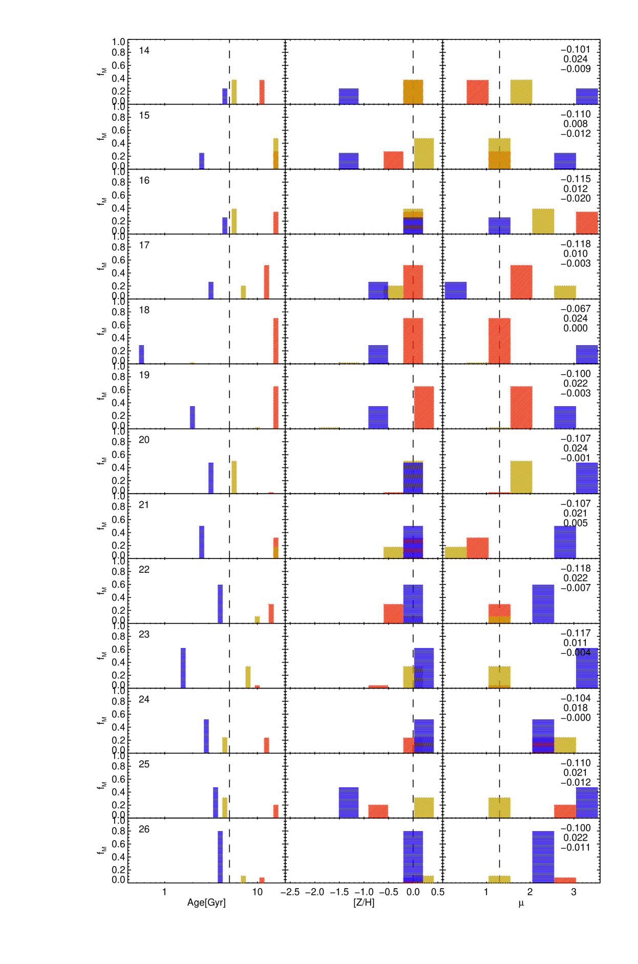
Figure 18: Continued

References

- Abazajian et al. (2009) Abazajian K. N., et al., 2009, ApJS, 182, 543
- Barmby & Huchra (2000) Barmby P., Huchra J. P., 2000, ApJ, 531, L29
- Barmby et al. (2000) Barmby P., Huchra J. P., Brodie J. P., Forbes D. A., Schroder L. L., Grillmair C. J., 2000, AJ, 119, 727
- Beasley et al. (2005) Beasley M. A., Brodie J. P., Strader J., Forbes D. A., Proctor R. N., Barmby P., Huchra J. P., 2005, AJ, 129, 1412
- Bertelli et al. (1994) Bertelli G., Bressan A., Chiosi C., Fagotto F., Nasi E., 1994, A&AS, 106, 275
- Bessell (1990) Bessell S., 1990, Pub. A.S.P., 102, 1181
- Bressan et al. (2006) Bressan A., et al., 2006, ApJ, 639, L55
- Bruzual & Charlot (2003) Bruzual G., Charlot S., 2003, MNRAS, 344, 1000
- Buser & Kurucz (1978) Buser R., Kurucz R. L., 1978, A&A, 70, 555
- Caldwell et al. (2011) Caldwell N., Schiavon R., Morrison H., Rose J. A., Harding P., 2011, AJ, 141, 61
- Cannon et al. (2006) Cannon R., et al., 2006, MNRAS, 372, 425
- Cardelli, Clayton, & Mathis (1989) Cardelli J. A., Clayton G. C., Mathis J. S., 1989, ApJ, 345, 245
- Carter, Visvanathan & Pickles (1986) Carter D., Visvanathan N., Pickles A. J., 1986, ApJ, 311, 637
- Cenarro et al. (2001a) Cenarro A. J., Cardiel N., Gorgas J., Peletier R. F., Vazdekis A., Prada F., 2001a, MNRAS, 326, 959
- Cenarro et al. (2001b) Cenarro A. J., Gorgas J., Cardiel N., Pedraz S., Peletier R. F., Vazdekis A., 2001b, MNRAS, 326, 981
- Cenarro et al. (2003) Cenarro A. J., Gorgas J., Vazdekis A., Cardiel N., Peletier R. F., 2003, MNRAS, 339, L12
- Cenarro et al. (2007) Cenarro A. J., et al., 2007, MNRAS, 374, 664
- Charlot & Fall (2000) Charlot S., Fall S. M., 2000, ApJ, 539, 718
- Coelho et al. (2005) Coelho P., Barbuy B., Meléndez J., Schiavon R. P., Castilho B. V., 2005, A&A, 443, 735
- Coelho et al. (2007) Coelho P., Bruzual G., Charlot S., Weiss A., Barbuy B., Ferguson J. W., 2007, MNRAS, 382, 498
- Conroy & Gunn (2010) Conroy C., Gunn J. E., 2010, ApJ, 712, 833
- De Angeli et al. (2005) De Angeli F., Piotto G., Cassisi S., Busso G., Recio-Blanco A., Salaris M., Aparicio A., Rosenberg A., 2005, AJ, 130, 116
- De Lucia et al. (2006) De Lucia G., Springel V., White S. D. M., Croton D., Kauffmann G., 2006, MNRAS, 366, 499
- Eisenstein et al. (2001) Eisenstein D. J., et al., 2001, AJ, 122, 2267
- Fan et al. (2008) Fan Z., Ma J., de Grijs R., Zhou X., 2008, MNRAS, 385, 1973
- Faber & French (1980) Faber S. M., French. H., 1980, ApJ, 235, 405
- Falcón-Barroso et al. (2011) Falcón-Barroso J., Sánchez-Blázquez P., Vazdekis A., Ricciardelli E., Cardiel N., Cenarro A. J., Gorgas J., Peletier R. F., 2011, A&A, 532, A95
- Fernie (1974) Fernie J. D., 1974, Pub. A.S.P., 86, 837
- Galleti et al. (2009) Galleti S., Bellazzini M., Buzzoni A., Federici L., Fusi Pecci F., 2009, A&A, 508, 1285
- Girardi et al. (2000) Girardi L., Bressan A., Bertelli G., Chiosi C., 2000, A&AS, 141, 371
- Hayes (1985) Hayes, D. S., 1985, in D. S. Hayes, L. E. Pasinetti, & A. G. D. Philip, eds. Proc. IAU Symposium 111, Calibration of fundamental stellar quantities. Dordrecht, Reidel, p. 225.
- Harris (1996) Harris W. E., 1996, AJ, 112, 1487
- Huchra, Brodie, & Kent (1991) Huchra J. P., Brodie J. P., Kent S. M., 1991, ApJ, 370, 495
- Johnson (1965) Johnson H. L., 1965, ApJ, 141, 923
- Kaviraj et al. (2007) Kaviraj S., et al., 2007, ApJS, 173, 619
- Lejeune, Cuisinier, & Buser (1998) Lejeune T., Cuisinier F., Buser R., 1998, A&AS, 130, 65
- Maraston (2005) Maraston C., 2005, MNRAS, 362, 799
- Maraston et al. (2011) Maraston C., Stromback G., Portsmouth I.-U. o., Kingdom U., 2011, arXiv, arXiv:1109.0543
- Maraston et al. (2009) Maraston C., Strömbäck G., Thomas D., Wake D. A., Nichol R. C., 2009, MNRAS, 394, L107
- Marín-Franch et al. (2009) Marín-Franch A., et al., 2009, ApJ, 694, 1498
- Mendel, Proctor, & Forbes (2007) Mendel J. T., Proctor R. N., Forbes D. A., 2007, MNRAS, 379, 1618
- Milone, Sansom, & Sánchez-Blázquez (2011) Milone A. D. C., Sansom A. E., Sánchez-Blázquez P., 2011, MNRAS, 414, 1227
- Nair & Abraham (2010) Nair P. B., Abraham R. G., 2010, ApJS, 186, 427
- Oke & Gunn (1983) Oke J. B., Gunn J. E., 1983, ApJ, 266, 713
- Pagel (1997) Pagel B. E. J., 1997, nceg.book,
- Peacock et al. (2011) Peacock M. B., Zepf S. E., Maccarone T. J., Kundu A., 2011, arXiv, arXiv:1105.3365
- Peacock et al. (2010) Peacock M. B., Maccarone T. J., Knigge C., Kundu A., Waters C. Z., Zepf S. E., Zurek D. R., 2010, MNRAS, 402, 803
- Perrett et al. (2002) Perrett K. M., Bridges T. J., Hanes D. A., Irwin M. J., Brodie J. P., Carter D., Huchra J. P., Watson F. G., 2002, AJ, 123, 2490
- Poole et al. (2010) Poole V., Worthey G., Lee H.-c., Serven J., 2010, AJ, 139, 809
- Pickles (1998) Pickles A. J., 1998, PASP, 110, 863
- Renzini (2006) Renzini A., 2006, ARA&A, 44, 141
- Ricciardelli & Franceschini (2010) Ricciardelli E., Franceschini A., 2010, A&A, 518, A14
- Rosenberg et al. (1999) Rosenberg A., Saviane I., Piotto G., Aparicio A., 1999, AJ, 118, 2306
- Sánchez-Blázquez et al. (2006) Sánchez-Blázquez P., et al., 2006, MNRAS, 371, 703
- Sánchez-Blázquez et al. (2006) Sánchez-Blázquez P., Gorgas J., Cardiel N., González J. J., 2006, A&A, 457, 809
- Sarzi et al. (2008) Sarzi M., et al., 2008, ASPC, 390, 218
- Schiavon (2007) Schiavon R. P., 2007, ApJS, 171, 146
- Schiavon et al. (2002) Schiavon R. P., Faber S. M., Rose J. A., Castilho B. V., 2002, ApJ, 580, 873
- Stoughton et al. (2002) Stoughton C., et al., 2002, AJ, 123, 485
- Tojeiro et al. (2011a) Tojeiro R., Percival W. J., Heavens A. F., Jimenez R., 2011a, MNRAS, 413, 434
- Tojeiro & Percival (2011b) Tojeiro R., Percival W. J., 2011b, MNRAS, 417, 1114
- Trager et al. (2000) Trager S. C., Faber S. M., Worthey G., González J. J., 2000, AJ, 120, 165
- Valdes et al. (2004) Valdes F., Gupta R., Rose J. A., Singh H. P., Bell D. J., 2004, ApJS, 152, 251
- van Dokkum & Conroy (2010) van Dokkum P. G., Conroy C., 2010, Nature, 468, 940
- Vazdekis et al. (2010) Vazdekis A., Sánchez-Blázquez P., Falcón-Barroso J., Cenarro A. J., Beasley M. A., Cardiel N., Gorgas J., Peletier R. F., 2010, MNRAS, 404, 1639
- Vazdekis et al. (2003) Vazdekis A., Cenarro A. J., Gorgas J., Cardiel N., Peletier R. F., 2003, MNRAS, 340, 1317
- Vazdekis (1999) Vazdekis A., 1999, ApJ, 513, 224
- Vazdekis et al. (1997) Vazdekis A., Peletier R. F., Beckman J. E., Casuso E., 1997, ApJS, 111, 203
- Vazdekis et al. (1996) Vazdekis A., Casuso E., Peletier R. F., Beckman J. E., 1996, ApJS, 106, 307
- Vazdekis et al. (2001) Vazdekis A., Salaris M., Arimoto N., Rose J. A., 2001, ApJ, 549, 274
- Vazdekis et al. (2012) Vazdekis A., Ricciardelli E., Cenarro A.J., Rivero-Gonzalez J.G., Diaz-Garcia L.A. and Falcón-Barroso J., 2012, MNRAS, in press
- Wake et al. (2005) Wake D. A., Collins C. A., Nichol R. C., Jones L. R., Burke D. J., 2005, ApJ, 627, 186
- Wake et al. (2006) Wake D. A., et al., 2006, MNRAS, 372, 537
- Worthey (1994) Worthey G., 1994, ApJS, 95, 107
- Worthey et al. (2005) Worthey G., España A., MacArthur L. A., Courteau S., 2005, ApJ, 631, 820
- Worthey, Faber, & Gonzalez (1992) Worthey G., Faber S. M., Gonzalez J. J., 1992, ApJ, 398, 69
- Yamada et al. (2006) Yamada Y., Arimoto N., Vazdekis A., Peletier R. F., 2006, ApJ, 637, 200