Projected Quasi-particle Perturbation theory

Abstract

The BCS and/or HFB theories are extended by treating the effect of four quasi-particle states perturbatively. The approach is tested on the pairing hamiltonian, showing that it combines the advantage of standard perturbation theory valid at low pairing strength and of non-perturbative approaches breaking particle number valid at higher pairing strength. Including the restoration of particle number, further improves the description of pairing correlation. In the presented test, the agreement between the exact solution and the combined perturbative + projection is almost perfect. The proposed method scales friendly when the number of particles increases and provides a simple alternative to other more complicated approaches.

I Introduction

Theories breaking explicitly the particle number, like Bardeen-Cooper-Schrieffer (BCS) or Hartree-Fock-Bogoliubov (HFB) are the simplest efficient ways to describe pairing correlations in physical systems. However, these theories suffer from some limitations especially when the number of particles becomes rather small as it is the case in mesoscopic systems like in nuclear physics Rin80 or condensed matter Von01 . The main difficulty is the sharp transition from normal to superfluid phases as the pairing strength increases. The second difficulty is a systematic underestimation of pairing correlations that increases when the particle number decreases.

In the last decades, several approaches have been used to overcome these difficulties. When the number of particle is small enough, the exact solution of the pairing problem is accessible by direct diagonalization of the Hamiltonian Vol01 ; Zel03 ; Vol07 and/or using the secular equation originally proposed by Richardson Ric64 ; Duk04 ; Van06 . Accurate description of the ground state energy of superfluid systems with larger particle number can be obtained using either Quantum Monte-Carlo technique (see for instance Cap98 ; Muk11 ) or extending quasi-particle theories using Variation After Projection approaches Die64 ; Hup11 (for recent applications see Rod07 ; Rod10 ; Hup12 ). All of these methods are however rather involved and demanding in terms of computational power. The aim of the present work is to show that a perturbative approach can eventually provide a simpler and yet accurate alternative to treat the pairing problem.

In the following, standard perturbation theory is first recalled. It is then explained how to take advantage of both perturbative approaches and BCS/HFB theory. The importance of particle number restoration is finally highlighted.

II Standard perturbation theory

Our starting point here is similar to the one used in refs. San08 ; Muk11 . We assume a two-body pairing hamiltonian given by:

$$H = \sum_{i=1}^{\Omega}\varepsilon_{i}(a^{\dagger}_{i}a_{i}+a^{\dagger}_{\bar{i}}a_{\bar{i}})+\sum_{i\neq j}^{\Omega}v_{ij}a^{\dagger}_{i}a^{\dagger}_{\bar{i}}a_{\bar{j}}a_{j}$$

$$\equiv H_{0}+V.$$

Here, $(i,{\bar{i}})$ denotes time-reversed pair. Such an hamiltonian can be for instance constructed starting from a realistic self-consistent mean-field calculation providing single-particle energies and two-body matrix elements Muk11 .

Here $\Omega$ denotes the maximal number of accessible levels for the pairs of particles. In the following, we will consider the specific case of equidistant levels with $\varepsilon_{i}=(i-1)\Delta\varepsilon$ with $\Delta\varepsilon=1$ MeV and a number of particles $N=\Omega$.

As already noted some times ago Bis71 and recently rediscussed Sch01 ; San08 , the two-body part $V$ can be treated perturbatively to provide an accurate description of the pairing problem in the weak pairing interaction regime. Starting from the ground state $|\Phi_{0}\rangle$ of $H_{0}$, that corresponds to the Slater determinant obtained by occupying the lowest single-particle states while other excited states $|\Phi_{n}\rangle$ of $H_{0}$ can be obtained by considering particle-hole (p-h), 2p-2h, … excitations built on top of the $|\Phi_{0}\rangle$. Using second-order perturbation theory, the ground state energy of $H$ reads:

$${\mathbf{E}}_{0} = E_{0}+E^{(2)}_{0}$$ (2)

where $E_{0}=2\sum_{i=1,N_{\rm pair}}\varepsilon_{i}$ (with $N_{\rm pair}=N/2$) is the ground state energy of $H_{0}$ while $E^{(2)}_{0}$ is the standard second-order correction, that can be found in textbook:

$$E^{(2)}_{0} = \sum_{n\neq 0}\frac{\left|\langle\Phi_{0}|V|\Phi_{n}\rangle\right|^{2}}{E_{0}-E_{n}}$$ (3)

In the specific case considered here, i.e. Eq. (II), only 2p-2h states contribute to the second order correction. More precisely, the states $n$ could only differ from the ground state by one occupied pair above the Fermi sea (denoted by $j$) and one unoccupied pair below (denoted by $i$): $|\Phi_{i,j}\rangle=a^{\dagger}_{j}a^{\dagger}_{\bar{j}}a_{\bar{i}}a_{i}|\Phi_{0}\rangle$ and are eigenstates of $H_{0}$ with energy $E_{ij}=E_{0}+2(\varepsilon_{j}-\varepsilon_{i})$. This leads to

$$E^{(2)}_{0}=-\frac{1}{2}\sum_{i=1,N_{\rm pair}}\sum_{j=N_{\rm pair}+1,N_{\rm max}}\frac{|v_{ij}|^{2}}{\varepsilon_{j}-\varepsilon_{i}},$$ (4)

with $N_{\rm pair}=N/2$ and $N_{\rm max}=\Omega/2$. This expression has been obtained in ref. Sch01 using a different approach based on the Richardson-Gaudin equation. It is known Bis71 ; San08 that standard perturbation theory provides an appropriate description in the weak coupling regime.

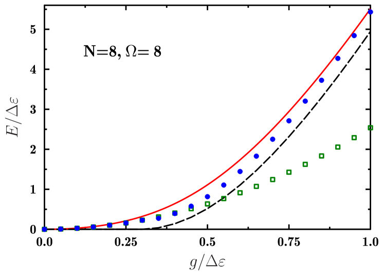
Figure 1: (color online) Illustration of the correlation energy as a function of the coupling strength for the case of N=8 particles and $\Omega=8$. The exact result solution (red solid curve), BCS (black dashed line), standard perturbation theory (green open squares), Eq. (3) and QP²T theory with second order correction Eq. (14) (blue filled circles), are displayed.

In figure 1, an example of standard perturbation theory (SPT) is presented for the $N=8$ particles and constant coupling case, i.e. $v_{ij}=-g$. The correlation energy defined as the difference between the Hartree-Fock energy $E_{0}$ and the ground state energy ${\mathbf{E}}_{0}$ obtained with STP are compared to the exact solution and BCS result. In the latter case, pairing correlation is non-zero only above the threshold value $g/\Delta\varepsilon\simeq 0.3$. As illustrated from Fig. 1, standard perturbation theory matches with the exact result below the threshold but significantly underestimates the correlation for larger $g$ value. This aspect underlines the highly non-perturbative nature of the pairing quantum phase-transition. On the opposite, one of the advantage a theory like BCS is the possibility to incorporate non-perturbative physics even in the strong interaction case by breaking the U(1) symmetry associated to particle number conservation.

III Quasi-particle Perturbation theory

To provide a proper description of both the weak and strong pairing strength regime, it seems quite natural to try to combine theories based on quasi-particles and perturbative approaches. This possibility has been explored long time ago in Refs. Bal62 ; Hen64 mainly to discuss the removal of ”dangerous diagram” occuring in normal perturbation theory. Note that recently, it has also been revisited as a possible tool to perform ab-initio calculation in nuclei Som11 based on Gorkov-Green function formalism Gor58 . In the following, it is assumed that the BCS/HFB approach has been applied in a preliminary study and that the hamiltonian (II) is written in the canonical basis of the quasi-particle ground state. Then, the ground state takes the form

$$|\Phi_{0}\rangle= = \prod_{i>0}\left(U_{i}+V_{i}a^{\dagger}_{i}a^{\dagger}_{\bar{i}}\right)|-\rangle,$$ (5)

and is the vacuum of the quasi-particle creation operators defined through:

$$\beta^{\dagger}_{i} = U_{i}a^{\dagger}_{i}-V_{i}a_{\bar{i}},$$ (6)

$$\beta^{\dagger}_{\bar{i}} = U_{i}a^{\dagger}_{\bar{i}}+V_{i}a_{i}.$$ (7)

In the HFB/BCS theory, the original hamiltonian is replaced by an effective Hamiltonian that is conveniently written as :

$$H_{0} = E_{0}+\sum_{i}E_{i}\left(\beta^{\dagger}_{i}\beta_{i}+\beta^{\dagger}_{\bar{i}}\beta_{\bar{i}}\right)$$ (8)

where $E_{0}$ is the BCS/HFB ground state energy, while $E_{i}$ corresponds to the quasi-particle energy given by:

$$E_{i} = \sqrt{(\varepsilon_{i}-\lambda)^{2}+\Delta^{2}}$$ (9)

where $\lambda$ is the Lagrange multiplier used to impose the average particle number while $\Delta$ is the pairing gap (for a detailed discussion see Bri05 ).

For even systems, excited states of $H_{0}$ are 2 quasi-particle (2QP), 4 quasi-particle (4QP), … excitations with respect to the ground state. The original hamiltonian $H$ contains many terms that are neglected in $H_{0}$ Rin80 and that are responsible from the deviation between the quasi-particle and the exact solution. However, noting that:

$$H|\Phi_{0}\rangle=\left(H_{0}-\sum_{i\neq j}v_{ij}U^{2}_{i}V^{2}_{j}\beta^{\dagger}_{i}\beta^{\dagger}_{\bar{i}}\beta^{\dagger}_{j}\beta^{\dagger}_{\bar{j}}\right)|\Phi_{0}\rangle,$$ (10)

it can be anticipated that the main source of discrepancy is due to the coupling of $\Phi_{0}$ with the 4QP states. Some arguments showing that 4QP states should improved the description of pairing especially in the weak coupling regime have been given in ref. Man66 .

Below, perturbation theory is applied assuming that $H_{0}$ (Eq. 8) is the unperturbed hamiltonian while the perturbation $V$ is given by:

$$V = -\sum_{i\neq j}v_{ij}U^{2}_{i}V^{2}_{j}\beta^{\dagger}_{i}\beta^{\dagger}_{\bar{i}}\beta^{\dagger}_{j}\beta^{\dagger}_{\bar{j}}.$$ (11)

$V$ couples the ground state with the 4QP states, defined as (for $i>j$):

$$|\Phi_{i,j}\rangle = \beta^{\dagger}_{i}\beta^{\dagger}_{\bar{i}}\beta^{\dagger}_{j}\beta^{\dagger}_{\bar{j}}|\Phi_{0}\rangle$$ (12)

and associated to the unperturbed energy

$$E_{ij}=E_{0}+2\left(E_{i}+E_{j}\right).$$ (13)

The present approach, that is a direct extension of standard perturbation theory, is called hereafter quasi-particle perturbation theory (QP²T). Using Eq. (3), the second order correction to the ground state energy is equal to:

$$E^{(2)}_{0} = -\frac{1}{2}\sum_{i>j}v^{2}_{ij}\frac{(U^{2}_{i}V^{2}_{j}+U^{2}_{j}V^{2}_{i})^{2}}{E_{i}+E_{j}}.$$ (14)

This correction properly extends Eq. (4) from the normal to the superfluid phase. Indeed at the threshold value of $g$, i.e. when $\Delta\rightarrow 0$, the 4QP states identify with 2p-2h excitations while:

$$E_{i}+E_{j} \rightarrow |\varepsilon_{i}-\lambda|+|\varepsilon_{j}-\lambda|=\varepsilon_{i}-\varepsilon_{j},$$ (15)

and the standard perturbation theory case is recovered.

The result obtained with the QP²T approach at second order in perturbation (14) are displayed in figure 1 with filled circles. Note that below the BCS threshold, standard perturbation theory is used. The present approach can be regarded as a rather academic exercise but it turns out to provide a very simple way to extend mean-field theory based on quasi-particle states. In particular, it avoids the threshold problem of the latter and improves the description of correlation in the intermediate and strong coupling case.

IV Effect of the restoration of particle number

Similarly to the original quasi-particle theory, the energy deduced from the QP²T contains spurious contribution coming from the fact that the perturbed state does not preserves particle number. Indeed, using standard formulas, to second order in perturbation, the ground state expresses as:

$$|\Psi_{0}\rangle = |\Psi^{(0)}_{0}\rangle+|\Psi^{(1)}_{0}\rangle+|\Psi^{(2)}_{0}\rangle...$$ (16)

$$= |\Phi_{0}\rangle+\sum_{i>j}c_{ij}|\Phi_{i,j}\rangle+\cdots$$

where $|\Psi^{(i)}_{0}\rangle$, $i=0$, $1$, … denotes the contribution to the state at $i^{th}$ order in perturbation and where

$$c_{ij} = -\frac{v_{ij}}{2}\frac{(U^{2}_{i}V^{2}_{j}+U^{2}_{j}V^{2}_{i})}{E_{i}+E_{j}}.$$ (17)

Above the BCS threshold, neither $|\Phi_{0}\rangle$ nor $|\Phi_{i,j}\rangle$ are eigenstates of the particle number operator.

The most direct way to remove spurious contributions due to the mixing of different particle number is to introduce the operator $P^{N}$

$${P}^{N}=\frac{1}{2\pi}\int_{0}^{2\pi}\!d{\varphi}\;\,e^{i\varphi(\hat{N}-N)}.$$ (18)

that projects onto particle number $N$.

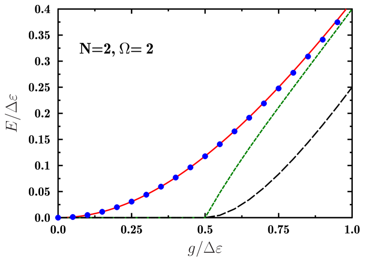
Figure 2: (color online) Illustration of the correlation energy as a function of the coupling strength for the case of N=2 particles and $\Omega=2$. The exact result solution (blue solid line), PAV result (green short-dashed line) and the combination of projection and perturbation theories (red filled circles) are shown. The original BCS (black long dashed line) is also shown as a reference.

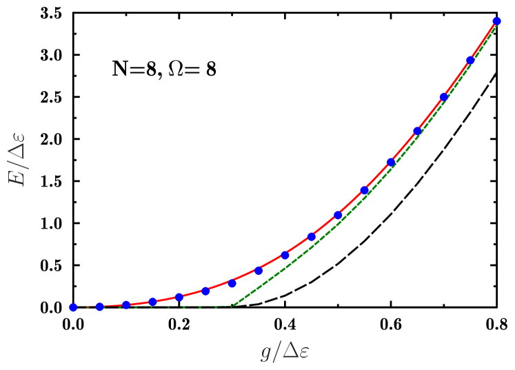
Figure 3: Same as figure 2 for the $N=\Omega=8$ case.

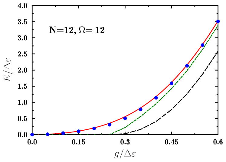
Figure 4: (color online) Same as figure 2 for the $N=\Omega=12$ case.

The most straightforward way to combine projection with quasi-particle perturbation theory is to directly take the expectation value

$${\rm\mathbf{E}}_{0} = \frac{\langle\Psi^{N}_{0}|H|\Psi^{N}_{0}\rangle}{\langle\Psi^{N}_{0}|\Psi^{N}_{0}\rangle}$$ (19)

with $|\Psi^{N}_{0}\rangle=P^{N}|\Psi_{0}\rangle$ and where $|\Psi_{0}\rangle$ is truncated at a given order in perturbation. This approach will be referred as the projected quasi-particle perturbation theory (QP³T) in the following. When only the zero order in perturbation is retained in Eq. (16), the QP³T identifies with the projection after variation (PAV) that is commonly used, especially in the nuclear Energy Density Functional approach (EDF) Ben03 . Formulas useful to compute the expectation values of one- and two-body operators with projection are given in appendix A. The projection is performed numerically using these expressions and the Fomenko discretization procedure of the gauge-space integrals Fom70 ; Ben09 . Here, $199$ discretization points have been used. Note that the number of points can be reduced down to $5$ without changing the result. The correlation energies obtained for $N=2$, $N=8$ and $N=12$ (each time with $\Omega=N$) using the second order QP³T are shown in figures 2, 3 and 4 respectively. In each case, the original BCS, the PAV and the exact solution are also shown. The result of QP³T almost superimposed with the exact solution. Only a slight difference can be seen around the BCS threshold.

Besides the energy, other observables can also be estimated. As an example, the quantity $n_{i}(1-n_{i})$ is shown in figure 5 as a function of single-particle energies, where $n_{i}$ are the occupation numbers of single-particle states. This quantity is a measure of the deviation from the independent particle picture where it is strictly zero for all states. The use of perturbation and projection considerably improves the description of one-body observables especially at intermediate coupling where the original BCS deviates significantly from the exact solution. In addition, even if the PAV differs significantly from the exact case as it was noted in ref. Hup11 , the extra mixing with the 4QP states compensates this drawback of PAV.

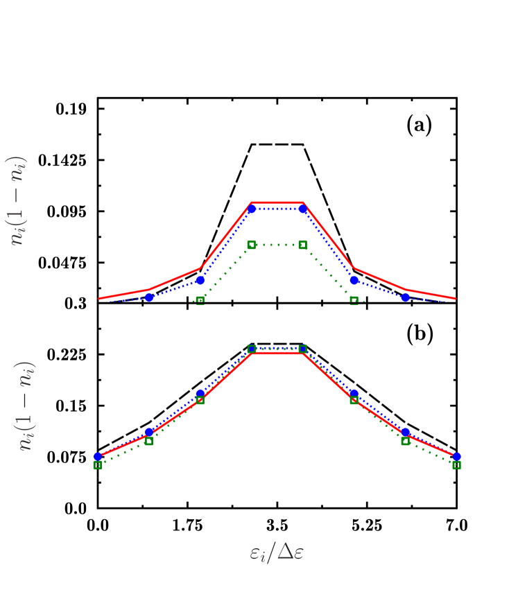
Figure 5: (color online) Example of evolution of the quantity $n_{i}(1-n_{i})$ obtained with QP³T (filled blue circles) as a function of single-particle energy for the $N=\Omega=8$ case with $g/\Delta\varepsilon=0.4$ (a) and $0.8$ (b). In both case, the exact result (red solid line) the BCS result (black dashed line) and the PAV result (green open squares) are shown.

In view of this agreement, it seems that the QP³T does automatically select important many-body states, namely projected ground state and projected 4QP states, on which the true eigenstate decomposes. These states are highly non-trivial multi-particle multi-hole mixing that can also be describe by direct diagonalization of the Hamiltonian but that is much more demanding numerically. Indeed, the size of the 4QP Hilbert space is $\Omega(\Omega-1)/2$ while the size of the matrix to diagonalize the hamiltonian is ($\Omega!/[N_{\rm pair}!(\Omega-N_{\rm pair})!]$). It is important to recall that here no diagonalization is required since the mixing coefficients are directly given by the quasi-particle perturbation theory, Eq. (17). These features make the approach rather simple to implement on existing HFB/BCS codes to provide a much better approximation than the PAV that is often currently used. In addition, by contrast to the Variation After Projection that is rather involved Rod07 ; Hup12 , no extra minimization is required.

Contrary to the exact diagonalization, the QP²T and QP³T can be performed even for large particle number. As an illustration, in figure 6, a systematic study of the correlation energy evolution obtained with some of the approaches presented above as the number of particle increases up to $N=100$ for the case $g/\Delta\varepsilon=0.8$. With standard diagonalization techniques, the exact solution can hardly be obtained for $N>14$. Other approaches based on quasi-particle theories can be applied without difficulties. Note however, that the QP³T requires to perform more and more gauge angles integrations (see appendix A) as $N$ increases making the calculations more time consuming with respect to the non-projected theories like BCS or QP²T.

From this figure, we also note that differences between theories are seen only for rather small particle number $N<30$, while above BCS and QP³T cannot be distinguished. However, as it has been discussed previously, for $N<30$, the QP³T is the only theory that can provide an excellent reproduction of the exact result when available.

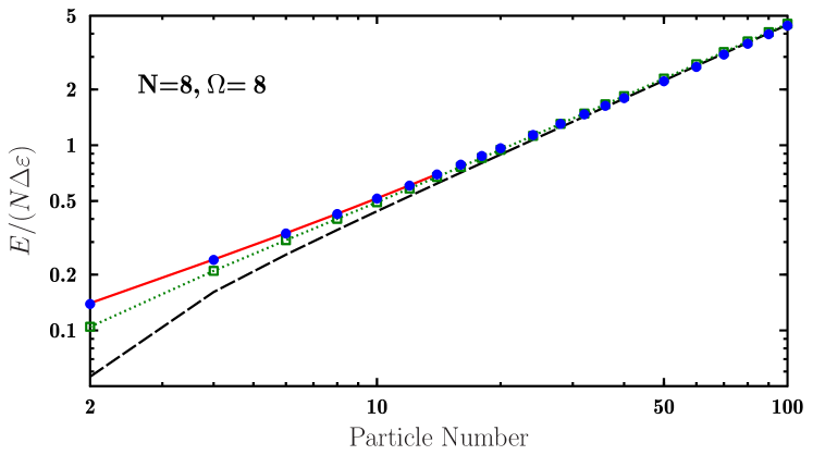
Figure 6: (color online) Evolution of the correlation energy per particle as a function of the number of particles for $g/\Delta\varepsilon=0.8$ for the BCS (black dashed line), QP²T (green open squares) and QP³T (blue filled circles). The exact case (solid red line) is also shown up to $N=14$ particles.

V Summary

In this work an extension of the standard many-body theory to treat the pairing problem is introduced. Including the effect of 4QP pertubatively to extend usual BCS/HFB removes the problem of sharp transition from normal to superfluid phase and significantly improves the description of pairing. Last, when restoration of particle number is performed within the perturbative approach, a perfect agreement with the exact results is found. This finding provide a direct proof of the importance of 4QP state to extend mean-field theories. In addition, it is shown that the quasi-particle perturbation theory can be implemented even for large particle number without special difficulties, making the technique rather attractive and much simpler than other approaches, like full diagonalization, variation after projection or Quantum Monte-Carlo techniques. Last, it is worth mentioning that the present technique can be directly and rather easily implemented on existing BCS/HFB codes Bon05 ; Doba04 to improve the description of pairing correlations.

Recently, the use of Gorkov-Green function theory has been proposed Som11 as a possible tool to perform ab-initio calculation for nuclei. This theory provides a general formalism based on quasi-particle states. The result obtained in the present study are rather encouraging to pursue in that direction and that projection might be needed.

Appendix A Expression of projected quantities

Starting from the standard expression of the quasi-particle ground state (Eq. (5)), the 4 QP states are given by:

$$|\Phi_{i,j}\rangle = \left(-V_{i}+U_{i}a^{\dagger}_{i}a^{\dagger}_{\bar{i}}\right)\left(-V_{j}+U_{j}a^{\dagger}_{j}a^{\dagger}_{\bar{j}}\right)$$ (20)

$$\prod_{k>0,k\neq(i,j)}\left(U_{k}+V_{k}a^{\dagger}_{k}a^{\dagger}_{\bar{k}}\right)|-\rangle.$$

For compactness, this expression is written as

$$|\Phi_{m}\rangle = \prod_{k>0}\left(U^{m}_{k}+V^{m}_{k}a^{\dagger}_{k}a^{\dagger}_{\bar{k}}\right)|-\rangle.$$ (21)

This notation includes the ground state case ($m=0$). The state obtained in QP³T can be generically written as $|\Psi^{N}_{0}\rangle=\sum_{m}c_{m}P_{N}|\Phi_{m}\rangle$, and for any operator $O$ that conserves the particle number, we have

$$\langle\Psi^{N}_{0}|O|\Psi^{N}_{0}\rangle=\sum_{m,n}c^{*}_{n}c_{m}\langle\Phi_{n}|OP^{N}|\Phi_{m}\rangle$$ (22)

where

$$\langle\Phi_{n}|OP^{N}|\Phi_{m}\rangle=\int_{0}^{2\pi}d\varphi\,\frac{e^{-i\varphi N}}{2\pi}\langle\Phi_{n}|O|\Phi_{m}(\varphi)\rangle,$$ (23)

and

$$|\Phi_{m}(\varphi)\rangle = \prod_{k>0}\left(U^{m}_{k}+V^{m}_{k}e^{2i\varphi}a^{\dagger}_{k}a^{\dagger}_{\bar{k}}\right)|-\rangle.$$ (24)

Starting from this expression it could be deduced that:

$$\langle\Phi_{n}|P^{N}|\Phi_{m}\rangle = \frac{1}{2\pi}\int_{0}^{2\pi}\!d{\varphi}e^{-i\varphi N}\prod_{k>0}\big{(}U^{n}_{k}U^{m}_{k}+V^{n}_{k}V^{m}_{k}e^{2i\varphi}\big{)}$$ (25)

$$\langle\Phi_{n}|a^{\dagger}_{i}a_{i}P^{N}|\Phi_{m}\rangle = \frac{1}{2\pi}\int_{0}^{2\pi}\!d{\varphi}e^{-i\varphi N}V^{n}_{i}V^{m}_{i}e^{2i\varphi}\prod_{k>0,k\neq i}\big{(}U^{n}_{k}U^{m}_{k}+V^{n}_{k}V^{m}_{k}e^{2i\varphi}\big{)}$$

$$\langle\Phi_{n}|a^{\dagger}_{i}a^{\dagger}_{\bar{i}}a_{\bar{j}}a_{j}P^{N}|\Phi_{m}\rangle = \frac{1}{2\pi}\int_{0}^{2\pi}\!d{\varphi}e^{-i\varphi N}V^{n}_{i}U^{m}_{i}U^{n}_{j}V^{m}_{j}e^{2i\varphi}\prod_{k>0,k\neq(i,j)}\big{(}U^{n}_{k}U^{m}_{k}+V^{n}_{k}V^{m}_{k}e^{2i\varphi}\big{)}$$

where the latter expression is valid for $i\neq j$.

References

- (1) P. Ring and P. Schuck, The Nuclear Many Body Problem (Springer-Verlag, New York, 1980).
- (2) J. von Delft and D. C. Ralf, Phys. Rep. 345, 61 (2001).
- (3) A. Volya, B. A. Brown and V. Zelevinsky, Phys. Lett. B 509, 37 (2001).
- (4) V. Zelevinsky and A. Volya, Phys. of Atomic Nuclei, 66, 1781 (2003).
- (5) T. Sumaryada and A. Volya, Phys. Rev. C 76, 024319 (2007).
- (6) R. W. Richardson and N. Sherman, Nucl. Phys. 52, 221 (1964); R. W. Richardson, Phys. Rev. 141, 949 (1966); J. Math. Phys. 9, 1327 (1968).
- (7) J. Dukelsky, S. Pittel, and G. Sierra, Rev. Mod. Phys. 76, 643 (2004)
- (8) K. Van Houcke, S. M. A. Rombouts, and L. Pollet Phys. Rev. E 73, 056703 (2006).
- (9) Abhishek Mukherjee, Y. Alhassid, and G. F. Bertsch, Phys. Rev. C83, 014319 (2011).
- (10) R. Capote, E. Mainegra, and A. Ventura, J. Phys. G 24, 1113 (1998).
- (11) K. Dietrich, H. J. Mang and J. H. Pradal, Phys. Rev. 135, B22 (1964).
- (12) G. Hupin and D. Lacroix, Phys. Rev. C83, 024317 (2011).
- (13) T. R. Rodriguez and J. L. Egido, Phys. Rev. Lett. 99, 062501 (2007).
- (14) T. R. Rodriguez and J. L. Egido, Phys. Rev. C 81, 064323 (2010).
- (15) G. Hupin and D. Lacroix, nucl-th/1205.0577v01.
- (16) N. Sandulescu and G. F. Bertsch, Phys. Rev. C 78, 064318 (2008).
- (17) M. Bishari, I. Unna, and A. Mann Phys. Rev. C 3, 1715 (1971).
- (18) M. Schechter, Y. Imry, Y. Levinson, and J. von Delft Phys. Rev. B 63, 214518 (2001).
- (19) D. M. Brink and R. A. Broglia, Nuclear Superfluidity: Pairing in Finite Systems (Cambridge University Press, 2005).
- (20) M. Bender and P.-H. Heenen and P.-G. Reinhard, Rev. Mod. Phys. 75, 121 (2003).
- (21) V. N. Fomenko, J. Phys. G 3, 8 (1970).
- (22) M. Bender, T. Duguet, and D. Lacroix, Phys. Rev. C 79, 044319 (2009).
- (23) P. Bonche, H. Flocard, and P.-H. Heenen, Comput. Phys. Commun. 171, 49 (2005).
- (24) J. Dobaczewski, P. Olbratowski, Comput. Phys. Comm. 158 (2004) 158.
- (25) E. M. Henley and L. Wilets, Phys. Rev. 133, B1118 (1964).
- (26) R. Balian and M. L. Metha, Nucl. Phys. 31, 587 (1962).
- (27) L. P. Gorkov, Sov. Phys. JETP 7, 505 (1958).
- (28) V. Soma, T. Duguet, and C. Barbieri, Phys. Rev. C 84, 064317 (2011).
- (29) Hans J. Mang, John O. Rasmussen, and Mannque Rho, Phys. Rev. 141, 941 (1966).