Joint Channel Estimation and Data Detection for Multihop OFDM Relaying System under Unknown Channel Orders and Doppler Frequencies

Rui Min and Yik-Chung Wu Rui Min and Yik-Chung Wu are with the Department of Electrical and Electronic Engineering, The University of Hong Kong, Pokfulam Road, Hong Kong. Email:{minrui,ycwu}@eee.hku.hk.The corresponding author is Yik-Chung Wu.
Abstract

In this paper, channel estimation and data detection for multihop relaying orthogonal frequency division multiplexing (OFDM) system is investigated under time-varying channel. Different from previous works, which highly depend on the statistical information of the doubly-selective channel (DSC) and noise to deliver accurate channel estimation and data detection results, we focus on more practical scenarios with unknown channel orders and Doppler frequencies. Firstly, we integrate the multilink, multihop channel matrices into one composite channel matrix. Then, we formulate the unknown channel using generalized complex exponential basis expansion model (GCE-BEM) with a large oversampling factor to introduce channel sparsity on delay-Doppler domain. To enable the identification of nonzero entries, sparsity enhancing Gaussian distributions with Gamma hyperpriors are adopted. An iterative algorithm is developed under variational inference (VI) framework. The proposed algorithm iteratively estimate the channel, recover the unknown data using Viterbi algorithm and learn the channel and noise statistical information, using only limited number of pilot subcarrier in one OFDM symbol. Simulation results show that, without any statistical information, the performance of the proposed algorithm is very close to that of the optimal channel estimation and data detection algorithm, which requires specific information on system structure, channel tap positions, channel lengths, Doppler shifts as well as noise powers.

Index Terms:
Doubly-selective channel, Channel estimation, Data detection, Variational inference, Orthogonal frequency division multiplexing, Multihop relaying system

I Introduction

Next generation broadband system aims to support higher levels of mobility, connectivity and efficiency. Multihop relaying system is a perfect suit for such requirement due to their benefits in easy deployment, enhanced connectivity, flexible adaptability, and increased capacity. On the other hand, orthogonal frequency division multiplexing (OFDM) has been adopted as the transmission scheme for many next generation broadband standards, such as WiMAX, LTE and IEEE 802.16. These result in the need to develop receiver algorithms for multihop OFDM system under high mobility. With high mobility, the broadband wireless channel is both frequency-selective and time-varying, a.k.a. doubly-selective. The channel responses vary sample by sample, which destroy the orthogonal property among subcarriers and causes intercarrier interference (ICI). Besides, the relaying system structure and channel statistical information are generally unknown to the receiver, due to flexible configuration of relaying paths. These poses strong challenges to channel estimation and data detection of OFDM relaying system under high mobility.

Over doubly-selective channel (DSC), channel estimation and data detection for single-hop OFDM systems has been considered in [1, 2, 3, 4, 5, 6], where the two tasks are treated separately. In [1, 2, 3, 4], the frequency domain channel matrix is approximated with a diagonal matrix under the assumption of small normalized Doppler frequency. The resulting algorithm would produce poor channel estimate and subsequently degrade the data detection performance for fast time-varying DSC. In view of that, [5] and [6] assumed a banded frequency-domain channel matrix, thus achieve a better channel modeling accuracy. However, due to the ICI introduced in frequency domain, pilots and data would interfere each other. This leads to the interdependence between channel estimation and data detection, and joint processing of them is necessary.

Research on multihop channel estimation is still limited especially for DSC, due to the complicated system structure and uncertain time-varying channel property. Among the limited existing works, [7] studied the two-way relaying (TWR) system under frequency-nonselective time-varying channel, and complex exponential basis expansion model (CE-BEM) was used to reduce the number of channel parameters. However, [7] only considered single carrier system and extension to multicarrier system is not straightforward due to additional ICI. More recently, in [8], an iterative algorithm for data detection and channel estimation was proposed for dual-hop amplify-and-forward (AF) OFDM system. With complete information of channel and noise in each hop, the data detection results were very close to the ideal case. Unfortunately, this work did not consider multihop relaying system, which has a more complicated structure. More importantly, it requires the destination receiver to have full statistical information of all channels and noise powers, which might not be readily available in practice.

In this paper, we study the channel estimation and data detection of OFDM-based multihop AF relaying system under high mobility, with special focus on unknown channel orders and Doppler frequencies. Based on the fact that the combined channel information is sufficient for data detection, and in order to reduce computation load on relays and time delay of the whole system, no channel estimation is performed at the relays. Different from previous works which highly rely on information of system structure, channel tap positions, channel lengths and Doppler frequencies of all channels, as well as noise powers at all receivers, we propose to solve the problems with none of the above information. By first expanding the composite source-relay-destination channel using generalized complex exponential basis expansion model (GCE-BEM) with a large oversampling factor, we introduce channel sparsity on delay-Doppler domain. Then sparsity enhancing Gaussian distributions with Gamma hyperpriors are adopted for channel estimation to enable the identification of nonzero elements. An iterative algorithm is proposed based on variational inference (VI) framework to iteratively estimate the channel, recover the unknown data using Viterbi algorithm and learn the channel and noise statistical information, using only limited number of pilot subcarrier in one OFDM symbol. Simulation results show that the performance of the proposed algorithm is very close to that of an optimal algorithm, which requires detailed statistical information on channels and noises.

The rest of the paper is organized as follows. The OFDM-based multihop relaying system is introduced in Section II. Then in Section III, the channel matrices of all the hops are integrated into one concise composite channel matrix and reformulated using GCE-BEM with a large oversampling factor. The iterative channel estimation and data detection algorithm is developed under VI framework in Section IV. And in Section V, least squares (LS) channel estimator and equalizer are derived to obtain the initial parameters for the proposed iterative algorithm. Simulation results of the proposed algorithm are presented in Section VI. Finally, this paper is concluded in Section VII.

Notations: Boldface uppercase and lowercase letters will be used for matrices and vectors, respectively. Superscripts H𝐻H, T𝑇T and * denote Hermitian, transpose and conjugate, respectively. The symbol 𝐈Nsubscript𝐈𝑁\mathbf{I}_{N} represents the N×N𝑁𝑁N\times N identity matrix. Symbol 𝐞lsubscript𝐞𝑙\mathbf{e}_{l} denotes the vector with structure given as [𝟎1×l,1,𝟎1×(Nl1)]Tsuperscriptsubscript01𝑙1subscript01𝑁𝑙1𝑇\left[\mathbf{0}_{1\times l},1,\mathbf{0}_{1\times(N-l-1)}\right]^{T}, where 𝟎1×lsubscript01𝑙\mathbf{0}_{1\times l} is the l𝑙l dimension all-zero row vector. diag{𝐱}diag𝐱\mathrm{diag}\{\mathbf{x}\} stands for the diagonal matrix with vector 𝐱𝐱\mathbf{x} on its diagonal. The notation [𝐗]m1:m2,n1:n2subscriptdelimited-[]𝐗:subscript𝑚1subscript𝑚2subscript𝑛1:subscript𝑛2[\mathbf{X}]_{m_{1}:m_{2},n_{1}:n_{2}} represents the submatrix of 𝐗𝐗\mathbf{X} consists of entries on the m1subscript𝑚1m_{1}-to-m2thsuperscriptsubscript𝑚2𝑡m_{2}^{th} rows and n1subscript𝑛1n_{1}-to-n2thsuperscriptsubscript𝑛2𝑡n_{2}^{th} columns. 𝔼{}𝔼\mathbb{E}\{\cdot\} denotes the expectation while Tr{𝐗}Tr𝐗\mathrm{Tr}\{\mathbf{X}\} and det{𝐗}det𝐗\mathrm{det}\{\mathbf{X}\} are the trace and the determinant of the square matrix 𝐗𝐗\mathbf{X}. Re{}Re\mathrm{Re}\{\cdot\} denotes the real part. And x𝑥\lceil x\rceil rounds x𝑥x to the nearest integer greater than or equal to x𝑥x. Finally, 𝐅𝐅\mathbf{F} represents the discrete Fourier transform (DFT) matrix with [𝐅]m,n=1Nej2πmn/Nsubscriptdelimited-[]𝐅𝑚𝑛1𝑁superscript𝑒𝑗2𝜋𝑚𝑛𝑁[\mathbf{F}]_{m,n}=\frac{1}{\sqrt{N}}e^{-j2\pi mn/N}.

II System Model

In this paper, we consider a multihop relaying system consists of a source 𝕊𝕊\mathbb{S}, a destination 𝔻𝔻\mathbb{D} and a number of relays scattered in the middle. Each of them is equipped with single antenna. Without loss of generality, we assume the relays work cooperatively to form K𝐾K links, each of them consisting of Υ+1Υ1\Upsilon+1 hops. Apart from the K𝐾K relaying paths, there is no other link between 𝕊𝕊\mathbb{S} and 𝔻𝔻\mathbb{D}, and all relays employ the AF scheme. Denoting the relay on the kthsuperscript𝑘𝑡{k^{th}} link connecting the ρthsuperscript𝜌𝑡\rho^{th} and the (ρ+1)thsuperscript𝜌1𝑡(\rho+1)^{th} hop as k,ρsubscript𝑘𝜌\mathbb{R}_{k,\rho}, the relaying system is shown in Figure 1.

The channel of each hop is assumed to be doubly-selective channel (DSC). Specifically, at the ρthsuperscript𝜌𝑡\rho^{th} hop of the kthsuperscript𝑘𝑡k^{th} relaying path, the channel consists of Nk,ρsubscript𝑁𝑘𝜌N_{k,\rho} independent nonzero channel taps with maximum delay of (Lmaxk,ρ1)Tssuperscriptsubscript𝐿𝑘𝜌1subscript𝑇𝑠(L_{\max}^{k,\rho}-1)T_{s}, where Tssubscript𝑇𝑠T_{s} is the sample interval. We consider the general situation that the channel taps are not necessarily consecutive, so that we have Nk,ρLmaxk,ρsubscript𝑁𝑘𝜌superscriptsubscript𝐿𝑘𝜌N_{k,\rho}\leq L_{\max}^{k,\rho}. Let h¯k,ρ(n,l)subscript¯𝑘𝜌𝑛𝑙\bar{h}_{k,\rho}(n,l) be the lthsuperscript𝑙𝑡l^{th} tap of that channel at time nTs𝑛subscript𝑇𝑠nT_{s}. For a given ρ𝜌\rho and k𝑘k, the channel taps are independent and each one being a zero-mean complex Gaussian process with bandlimited power spectral density within [fk,ρ(l),fk,ρ(l)]subscript𝑓𝑘𝜌𝑙subscript𝑓𝑘𝜌𝑙[-f_{k,\rho}(l),f_{k,\rho}(l)], where fk,ρ(l)subscript𝑓𝑘𝜌𝑙f_{k,\rho}(l) is the maximum Doppler shift of the lthsuperscript𝑙𝑡l^{th} tap. In general, fk,ρ(l)subscript𝑓𝑘𝜌𝑙f_{k,\rho}(l) may be distinct for different l𝑙l, since each tap results from signal transmission through a different physical scattering. Furthermore, it is assumed that the channels for different links k𝑘k and hops ρ𝜌\rho are independent from each other.

II-A OFDM Signal Transmitted from 𝕊𝕊\mathbb{S}

In an OFDM system, the frequency domain source data 𝐱=[x(0),,x(N1)]T𝐱superscript𝑥0𝑥𝑁1𝑇\mathbf{x}=[x(0),\ldots,x(N-1)]^{T} is first transformed to the time domain data 𝐬=𝐅H𝐱𝐬superscript𝐅𝐻𝐱\mathbf{s=F}^{H}\mathbf{x}, where 𝐅𝐅\mathbf{F} represents the discrete Fourier transform (DFT) matrix. In order to facilitate channel estimation and data detection, pilots are inserted in the frequency domain as

x(n)={xp(n)npxd(n)nd,𝑥𝑛casessubscript𝑥𝑝𝑛for-all𝑛subscript𝑝subscript𝑥𝑑𝑛for-all𝑛subscript𝑑x(n)=\left\{\begin{array}[]{ccc}x_{p}(n)&\forall&n\in\mathfrak{I}_{p}\\ x_{d}(n)&\forall&n\in\mathfrak{I}_{d},\end{array}\right. (1)

where dsubscript𝑑\mathfrak{I}_{d} is the index set of the Ndsubscript𝑁𝑑N_{d} unknown data symbols, psubscript𝑝\mathfrak{I}_{p} is the index set of the Npsubscript𝑁𝑝N_{p} pilot symbols and we have N=Nd+Np𝑁subscript𝑁𝑑subscript𝑁𝑝N=N_{d}+N_{p}. In matrix form, 𝐱𝐱\mathbf{x} can be represented as

𝐱=𝐄d𝐱d+𝐄p𝐱p,𝐱subscript𝐄𝑑subscript𝐱𝑑subscript𝐄𝑝subscript𝐱𝑝\mathbf{x=E}_{d}\mathbf{x}_{d}+\mathbf{E}_{p}\mathbf{x}_{p}, (2)

where 𝐄dsubscript𝐄𝑑\mathbf{E}_{d} and 𝐄psubscript𝐄𝑝\mathbf{E}_{p}, with dimensions N×Nd𝑁subscript𝑁𝑑N\times N_{d} and N×Np𝑁subscript𝑁𝑝N\times N_{p}, respectively, map 𝐱dsubscript𝐱𝑑\mathbf{x}_{d} and 𝐱psubscript𝐱𝑝\mathbf{x}_{p} to their corresponding subcarriers. Before transmission, a Cyclic Prefix (CP) of length Lcpsubscript𝐿𝑐𝑝L_{cp} is added at the beginning of 𝐬𝐬\mathbf{s} to prevent intersymbol interference (ISI). Since the OFDM signal goes through a number of relays before reaching the destination, Lcpsubscript𝐿𝑐𝑝L_{cp} should be larger than the maximum channel length among all the relaying paths, denoted as Lmax=maxk(ρ=1Υ+1Lmaxk,ρΥ)subscript𝐿subscript𝑘superscriptsubscript𝜌1Υ1subscriptsuperscript𝐿𝑘𝜌ΥL_{\max}=\max\limits_{k}(\sum_{\rho=1}^{\Upsilon+1}L^{k,\rho}_{\max}-\Upsilon).

II-B Received OFDM Signal

In AF relaying system, each relay merely amplify the received signal before passing the signal to the next relay or destination. For the kthsuperscript𝑘𝑡{k^{th}} relaying path, the signal received at k,1subscript𝑘1\mathbb{R}_{k,1} is given by

rk,1(n)=l=0Lmaxk,11h¯k,1(n,l)s(nl)+wk,1(n),subscript𝑟𝑘1𝑛superscriptsubscript𝑙0superscriptsubscript𝐿𝑘11subscript¯𝑘1𝑛𝑙𝑠𝑛𝑙subscript𝑤𝑘1𝑛r_{k,1}(n)=\sum_{l=0}^{L_{\max}^{k,1}-1}\bar{h}_{k,1}(n,l)s(n-l)+w_{k,1}(n), (3)

where wk,1(n)subscript𝑤𝑘1𝑛w_{k,1}(n) is the additive white Gaussian noise (AWGN) with power ϖk,12superscriptsubscriptitalic-ϖ𝑘12\varpi_{k,1}^{2}. Upon receiption, the relay amplifies the incoming signal as [9]

zk,1(n)=ςk,1rk,1(n)subscript𝑧𝑘1𝑛subscript𝜍𝑘1subscript𝑟𝑘1𝑛z_{k,1}(n)=\varsigma_{k,1}r_{k,1}(n) (4)

and then transmits zk,1(n)subscript𝑧𝑘1𝑛z_{k,1}(n) to the next relay k,2subscript𝑘2\mathbb{R}_{k,2} through channel h¯k,2(n,l)subscript¯𝑘2𝑛𝑙\bar{h}_{k,2}(n,l). The received signal is then represented as

rk,2(n)=l=0Lmaxk,21h¯k,2(n,l)zk,1(nl)+wk,2(n),subscript𝑟𝑘2𝑛superscriptsubscript𝑙0superscriptsubscript𝐿𝑘21subscript¯𝑘2𝑛𝑙subscript𝑧𝑘1𝑛𝑙subscript𝑤𝑘2𝑛r_{k,2}(n)=\sum_{l=0}^{L_{\max}^{k,2}-1}\bar{h}_{k,2}(n,l)z_{k,1}(n-l)+w_{k,2}(n), (5)

with wk,2(n)subscript𝑤𝑘2𝑛w_{k,2}(n) being the AWGN with power ϖk,22superscriptsubscriptitalic-ϖ𝑘22\varpi_{k,2}^{2}. The signal is then amplified as zk,2(n)=ςk,2rk,2(n)subscript𝑧𝑘2𝑛subscript𝜍𝑘2subscript𝑟𝑘2𝑛z_{k,2}(n)=\varsigma_{k,2}r_{k,2}(n) and transmitted to k,3subscript𝑘3\mathbb{R}_{k,3} and so on. Then, at the ΥthsuperscriptΥ𝑡\Upsilon^{th} relay, the amplified signal is transmitted to the destination. Finally at destination 𝔻𝔻\mathbb{D}, the received signal is given by

y~(n)=k=1Kl=0Lmaxk,Υ+11h¯k,Υ+1(n,l)zk,Υ(nl)+wd(n),~𝑦𝑛superscriptsubscript𝑘1𝐾superscriptsubscript𝑙0superscriptsubscript𝐿𝑘Υ11subscript¯𝑘Υ1𝑛𝑙subscript𝑧𝑘Υ𝑛𝑙subscript𝑤𝑑𝑛\tilde{y}(n)=\sum_{k=1}^{K}\sum_{l=0}^{L_{\max}^{k,\Upsilon+1}-1}\bar{h}_{k,\Upsilon+1}(n,l)z_{k,\Upsilon}(n-l)+w_{d}(n), (6)

where AWGN wd(n)subscript𝑤𝑑𝑛w_{d}(n) has power ϖd2superscriptsubscriptitalic-ϖ𝑑2\varpi_{d}^{2}. Upon reception, the CP [y~(Lcp),,y~(1)]Tsuperscript~𝑦subscript𝐿𝑐𝑝~𝑦1𝑇[\tilde{y}(-L_{cp}),\ldots,\tilde{y}(-1)]^{T} is removed and the received signal 𝐲~=[y~(0),,y~(N1)]N~𝐲superscript~𝑦0~𝑦𝑁1𝑁\mathbf{\tilde{y}}=[\tilde{y}(0),\ldots,\tilde{y}(N-1)]^{N} can be written in matrix form as

𝐲~=k=1K𝐇¯k,Υ+1𝐳k,Υ+𝐰d,~𝐲superscriptsubscript𝑘1𝐾subscript¯𝐇𝑘Υ1subscript𝐳𝑘Υsubscript𝐰𝑑\mathbf{\tilde{y}}=\sum_{k=1}^{K}\mathbf{\bar{H}}_{k,\Upsilon+1}\mathbf{z}_{k,\Upsilon}+\mathbf{w}_{d}, (7)

where 𝐳k,Υ=[zk,Υ((Lmaxk,Υ+11)),,zk,Υ(0),,zk,Υ(N1)]Tsubscript𝐳𝑘Υsuperscriptsubscript𝑧𝑘Υsuperscriptsubscript𝐿𝑘Υ11subscript𝑧𝑘Υ0subscript𝑧𝑘Υ𝑁1𝑇\mathbf{z}_{k,\Upsilon}=[z_{k,\Upsilon}(-(L_{\max}^{k,\Upsilon+1}-1)),\ldots,z_{k,\Upsilon}(0),\ldots,z_{k,\Upsilon}(N-1)]^{T}, 𝐰dsubscript𝐰𝑑\mathbf{w}_{d} is the noise vector with elements wd(n)subscript𝑤𝑑𝑛w_{d}(n), and 𝐇¯k,Υ+1subscript¯𝐇𝑘Υ1\mathbf{\bar{H}}_{k,\Upsilon+1} is an N×(N+Lmaxk,Υ+11)𝑁𝑁superscriptsubscript𝐿𝑘Υ11N\times(N+L_{\max}^{k,\Upsilon+1}-1) channel matrix given by

𝐇¯k,Υ+1=[h¯k,Υ+1(0,Lmaxk,Υ+11)h¯k,Υ+1(0,0)h¯k,Υ+1(1,Lmaxk,Υ+11)h¯k,Υ+1(1,0)h¯k,Υ+1(N1,Lmaxk,Υ+11)h¯k,Υ+1(N1,0)].subscript¯𝐇𝑘Υ1delimited-[]subscript¯𝑘Υ10superscriptsubscript𝐿𝑘Υ11subscript¯𝑘Υ100subscript¯𝑘Υ11superscriptsubscript𝐿𝑘Υ11subscript¯𝑘Υ110subscript¯𝑘Υ1𝑁1superscriptsubscript𝐿𝑘Υ11subscript¯𝑘Υ1𝑁10\mathbf{\bar{H}}_{k,\Upsilon+1}=\left[\begin{array}[]{l}\bar{h}_{k,\Upsilon+1}(0,L_{\max}^{k,\Upsilon+1}-1)\qquad\ldots\qquad\bar{h}_{k,\Upsilon+1}(0,0)\\ \quad\bar{h}_{k,\Upsilon+1}(1,L_{\max}^{k,\Upsilon+1}-1)\qquad\ldots\qquad\bar{h}_{k,\Upsilon+1}(1,0)\\ \qquad\quad\quad\quad\qquad\qquad\qquad\qquad\cdots\\ \qquad\quad\bar{h}_{k,\Upsilon+1}(N-1,L_{\max}^{k,\Upsilon+1}-1)\quad\ldots\quad\bar{h}_{k,\Upsilon+1}(N-1,0)\end{array}\right]. (8)

Furthermore, 𝐳k,Υsubscript𝐳𝑘Υ\mathbf{z}_{k,\Upsilon} can be written in terms of 𝐳k,Υ1subscript𝐳𝑘Υ1\mathbf{z}_{k,\Upsilon-1} as

𝐳k,Υ=ςk,Υ𝐇¯k,Υ𝐳k,Υ1+ςk,Υ𝐰k,Υ,subscript𝐳𝑘Υsubscript𝜍𝑘Υsubscript¯𝐇𝑘Υsubscript𝐳𝑘Υ1subscript𝜍𝑘Υsubscript𝐰𝑘Υ\mathbf{z}_{k,\Upsilon}=\varsigma_{k,\Upsilon}\mathbf{\bar{H}}_{k,\Upsilon}\mathbf{z}_{k,\Upsilon-1}+\varsigma_{k,\Upsilon}\mathbf{w}_{k,\Upsilon}, (9)

with 𝐳k,Υ1=[zk,Υ1((Lmaxk,Υ+1+Lmaxk,Υ)+2),,zk,Υ1(0),,zk,Υ1(N1)]Tsubscript𝐳𝑘Υ1superscriptsubscript𝑧𝑘Υ1superscriptsubscript𝐿𝑘Υ1superscriptsubscript𝐿𝑘Υ2subscript𝑧𝑘Υ10subscript𝑧𝑘Υ1𝑁1𝑇\mathbf{z}_{k,\Upsilon-1}=[z_{k,\Upsilon-1}(-(L_{\max}^{k,\Upsilon+1}+L_{\max}^{k,\Upsilon})+2),\ldots,z_{k,\Upsilon-1}(0),\ldots,z_{k,\Upsilon-1}(N-1)]^{T}, 𝐰k,Υsubscript𝐰𝑘Υ\mathbf{w}_{k,\Upsilon} is the corresponding noise vector, and 𝐇¯k,Υsubscript¯𝐇𝑘Υ\mathbf{\bar{H}}_{k,\Upsilon} is an (N+Lmaxk,Υ+11)×(N+Lmaxk,Υ+1+Lmaxk,Υ2)𝑁superscriptsubscript𝐿𝑘Υ11𝑁superscriptsubscript𝐿𝑘Υ1superscriptsubscript𝐿𝑘Υ2(N+L_{\max}^{k,\Upsilon+1}-1)\times(N+L_{\max}^{k,\Upsilon+1}+L_{\max}^{k,\Upsilon}-2) matrix given by

𝐇¯k,Υ=[h¯k,Υ(1Lmaxk,Υ+1,Lmaxk,Υ1)h¯k,Υ(1Lmaxk,Υ+1,0)h¯k,Υ(2Lmaxk,Υ+1,Lmaxk,Υ1)h¯k,Υ(2Lmaxk,Υ+1,0)h¯k,Υ(N1,Lmaxk,Υ1)h¯k,Υ(N1,0)].subscript¯𝐇𝑘Υdelimited-[]subscript¯𝑘Υ1superscriptsubscript𝐿𝑘Υ1superscriptsubscript𝐿𝑘Υ1subscript¯𝑘Υ1superscriptsubscript𝐿𝑘Υ10subscript¯𝑘Υ2superscriptsubscript𝐿𝑘Υ1superscriptsubscript𝐿𝑘Υ1subscript¯𝑘Υ2superscriptsubscript𝐿𝑘Υ10subscript¯𝑘Υ𝑁1superscriptsubscript𝐿𝑘Υ1subscript¯𝑘Υ𝑁10\mathbf{\bar{H}}_{k,\Upsilon}=\left[\begin{array}[]{l}\bar{h}_{k,\Upsilon}(1-L_{\max}^{k,\Upsilon+1},L_{\max}^{k,\Upsilon}-1)\qquad\ldots\qquad\bar{h}_{k,\Upsilon}(1-L_{\max}^{k,\Upsilon+1},0)\\ \quad\bar{h}_{k,\Upsilon}(2-L_{\max}^{k,\Upsilon+1},L_{\max}^{k,\Upsilon}-1)\qquad\ldots\qquad\bar{h}_{k,\Upsilon}(2-L_{\max}^{k,\Upsilon+1},0)\\ \qquad\qquad\quad\quad\quad\qquad\qquad\qquad\qquad\cdots\\ \qquad\quad\qquad\qquad\bar{h}_{k,\Upsilon}(N-1,L_{\max}^{k,\Upsilon}-1)\quad\ldots\quad\bar{h}_{k,\Upsilon}(N-1,0)\end{array}\right]. (10)

Tracing back to the 1stsuperscript1𝑠𝑡1^{st} hop, we have 𝐳k,1=ςk,1𝐇¯k,1𝐬k+ςk,1𝐰k,1subscript𝐳𝑘1subscript𝜍𝑘1subscript¯𝐇𝑘1subscript𝐬𝑘subscript𝜍𝑘1subscript𝐰𝑘1\mathbf{z}_{k,1}=\varsigma_{k,1}\mathbf{\bar{H}}_{k,1}\mathbf{s}_{k}+\varsigma_{k,1}\mathbf{w}_{k,1}, where 𝐇¯k,1subscript¯𝐇𝑘1\mathbf{\bar{H}}_{k,1} is an (N+ρ=2Υ+1Lmaxk,ρΥ)×(N+ρ=1Υ+1Lmaxk,ρΥ1)𝑁superscriptsubscript𝜌2Υ1superscriptsubscript𝐿𝑘𝜌Υ𝑁superscriptsubscript𝜌1Υ1superscriptsubscript𝐿𝑘𝜌Υ1(N+\sum_{\rho=2}^{\Upsilon+1}L_{\max}^{k,\rho}-\Upsilon)\times(N+\sum_{\rho=1}^{\Upsilon+1}L_{\max}^{k,\rho}-\Upsilon-1) channel matrix with structure the same as (8) and (10), and 𝐬k=𝐄k𝐬subscript𝐬𝑘subscript𝐄𝑘𝐬\mathbf{s}_{k}=\mathbf{E}_{k}\mathbf{s} with 𝐄k=[[𝐈N]1:N,(Nρ=1Υ+1Lmaxk,ρ+Υ+2):N,𝐈N]Tsubscript𝐄𝑘superscriptsubscriptdelimited-[]subscript𝐈𝑁:1𝑁𝑁superscriptsubscript𝜌1Υ1superscriptsubscript𝐿𝑘𝜌Υ2:𝑁subscript𝐈𝑁𝑇\mathbf{E}_{k}=[[\mathbf{I}_{N}]_{1:N,(N-\sum_{\rho=1}^{\Upsilon+1}L_{\max}^{k,\rho}+\Upsilon+2):N},\mathbf{I}_{N}]^{T} characterizing the effect of the CP. Based on the above derivations, the received signal vector 𝐲~~𝐲\mathbf{\tilde{y}} is

𝐲~~𝐲\displaystyle\mathbf{\tilde{y}} =\displaystyle= k=1K[(ρ=1Υςk,ρ)(𝐇¯k,Υ+1𝐇¯k,1)𝐄k]𝐇𝐅H𝐱subscriptsuperscriptsubscript𝑘1𝐾delimited-[]superscriptsubscriptproduct𝜌1Υsubscript𝜍𝑘𝜌subscript¯𝐇𝑘Υ1subscript¯𝐇𝑘1subscript𝐄𝑘absent𝐇superscript𝐅𝐻𝐱\displaystyle\underbrace{\sum_{k=1}^{K}\left[\left(\prod_{\rho=1}^{\Upsilon}\varsigma_{k,\rho}\right)\left(\mathbf{\bar{H}}_{k,\Upsilon+1}\ldots\mathbf{\bar{H}}_{k,1}\right)\mathbf{E}_{k}\right]}_{\triangleq\mathbf{H}}\mathbf{F}^{H}\mathbf{x} (11)
+k=1K[ρ=1Υ((ϱ=ρΥςk,ϱ)(𝐇¯k,Υ+1𝐇¯k,ρ+1))𝐰k,ρ]+𝐰d𝐯~,subscriptsuperscriptsubscript𝑘1𝐾delimited-[]superscriptsubscript𝜌1Υsuperscriptsubscriptproductitalic-ϱ𝜌Υsubscript𝜍𝑘italic-ϱsubscript¯𝐇𝑘Υ1subscript¯𝐇𝑘𝜌1subscript𝐰𝑘𝜌subscript𝐰𝑑absent~𝐯\displaystyle+\underbrace{\sum_{k=1}^{K}\left[\sum_{\rho=1}^{\Upsilon}\left(\left(\prod_{\varrho=\rho}^{\Upsilon}\varsigma_{k,\varrho}\right)\left(\mathbf{\bar{H}}_{k,\Upsilon+1}\ldots\mathbf{\bar{H}}_{k,\rho+1}\right)\right)\mathbf{w}_{k,\rho}\right]+\mathbf{w}_{d}}_{\triangleq\mathbf{\tilde{v}}},

where 𝐇𝐇\mathbf{H} represents the composite channel matrix and 𝐯~~𝐯\mathbf{\tilde{v}} represents the composite noise effect.

III Reformulation of the Composite Channel Matrix

In order to estimate the channel and detect the data, it is important to investigate the structure of the channel matrix 𝐇𝐇\mathbf{H}. Writing 𝐇=k=1K(ρ=1Υςk,ρ)𝐇k𝐇superscriptsubscript𝑘1𝐾superscriptsubscriptproduct𝜌1Υsubscript𝜍𝑘𝜌subscript𝐇𝑘\mathbf{H}=\sum_{k=1}^{K}\left(\prod_{\rho=1}^{\Upsilon}\varsigma_{k,\rho}\right)\mathbf{H}_{k}, where 𝐇k=𝐇¯k,Υ+1𝐇¯k,Υ𝐇¯k,1𝐄ksubscript𝐇𝑘subscript¯𝐇𝑘Υ1subscript¯𝐇𝑘Υsubscript¯𝐇𝑘1subscript𝐄𝑘\mathbf{H}_{k}=\mathbf{\bar{H}}_{k,\Upsilon+1}\mathbf{\bar{H}}_{k,\Upsilon}\ldots\mathbf{\bar{H}}_{k,1}\mathbf{E}_{k}. To find out the structure of 𝐇¯k,Υ+1𝐇¯k,Υ𝐇¯k,1𝐄ksubscript¯𝐇𝑘Υ1subscript¯𝐇𝑘Υsubscript¯𝐇𝑘1subscript𝐄𝑘\mathbf{\bar{H}}_{k,\Upsilon+1}\mathbf{\bar{H}}_{k,\Upsilon}\ldots\mathbf{\bar{H}}_{k,1}\mathbf{E}_{k}, we start from 𝐇¯k,Υ+1subscript¯𝐇𝑘Υ1\mathbf{\bar{H}}_{k,\Upsilon+1} and 𝐇¯k,Υsubscript¯𝐇𝑘Υ\mathbf{\bar{H}}_{k,\Upsilon} with their expressions given in (8) and (10), respectively. Each matrix represents the linear convolution of a time-varying channel and the matrix multiplication expresses the convolution effect of two time-varying channels. Therefore the resulting matrix 𝐇¯k,Υ+1𝐇¯k,Υsubscript¯𝐇𝑘Υ1subscript¯𝐇𝑘Υ\mathbf{\bar{H}}_{k,\Upsilon+1}\mathbf{\bar{H}}_{k,\Upsilon} will also be in the form of (8) and (10), except that the resulting channel length of the new time-varying channel is now being Lmaxk,Υ+1+Lmaxk,Υ1superscriptsubscript𝐿𝑘Υ1superscriptsubscript𝐿𝑘Υ1L_{\max}^{k,\Upsilon+1}+L_{\max}^{k,\Upsilon}-1.

Similarly, multiplying 𝐇¯k,Υ1subscript¯𝐇𝑘Υ1\mathbf{\bar{H}}_{k,\Upsilon-1} to 𝐇¯k,Υ+1𝐇¯k,Υsubscript¯𝐇𝑘Υ1subscript¯𝐇𝑘Υ\mathbf{\bar{H}}_{k,\Upsilon+1}\mathbf{\bar{H}}_{k,\Upsilon} from the right, the result 𝐇¯k,Υ+1𝐇¯k,Υ𝐇¯k,Υ1subscript¯𝐇𝑘Υ1subscript¯𝐇𝑘Υsubscript¯𝐇𝑘Υ1\mathbf{\bar{H}}_{k,\Upsilon+1}\mathbf{\bar{H}}_{k,\Upsilon}\mathbf{\bar{H}}_{k,\Upsilon-1} will be an N×(N+ρ=Υ1Υ+13)𝑁𝑁superscriptsubscript𝜌Υ1Υ13N\times(N+\sum_{\rho=\Upsilon-1}^{\Upsilon+1}-3) matrix, with equivalent channel length of ρ=Υ1Υ+1Lmaxk,ρ2superscriptsubscript𝜌Υ1Υ1superscriptsubscript𝐿𝑘𝜌2\sum_{\rho=\Upsilon-1}^{\Upsilon+1}L_{\max}^{k,\rho}-2, due to the convolution effect. Continuing the matrix multiplication, we have 𝐇¯k,Υ+1𝐇¯k,1subscript¯𝐇𝑘Υ1subscript¯𝐇𝑘1\mathbf{\bar{H}}_{k,\Upsilon+1}\ldots\mathbf{\bar{H}}_{k,1} being an N×(N+ρ=1Υ+1Lmaxk,ρΥ1)𝑁𝑁superscriptsubscript𝜌1Υ1superscriptsubscript𝐿𝑘𝜌Υ1N\times(N+\sum_{\rho=1}^{\Upsilon+1}L_{\max}^{k,\rho}-\Upsilon-1) matrix, with equivalent channel length of ρ=1Υ+1Lmaxk,ρΥsuperscriptsubscript𝜌1Υ1superscriptsubscript𝐿𝑘𝜌Υ\sum_{\rho=1}^{\Upsilon+1}L_{\max}^{k,\rho}-\Upsilon. And eventually 𝐄ksubscript𝐄𝑘\mathbf{E}_{k} moves the ρ=1Υ+1Lmaxk,ρΥ1superscriptsubscript𝜌1Υ1superscriptsubscript𝐿𝑘𝜌Υ1\sum_{\rho=1}^{\Upsilon+1}L_{\max}^{k,\rho}-\Upsilon-1 columns from the left part of 𝐇¯k,Υ+1𝐇¯k,1subscript¯𝐇𝑘Υ1subscript¯𝐇𝑘1\mathbf{\bar{H}}_{k,\Upsilon+1}\ldots\mathbf{\bar{H}}_{k,1} to the upper right corner. The resulted composite channel matrix 𝐇ksubscript𝐇𝑘{\mathbf{H}}_{k} is an N×N𝑁𝑁N\times N circular convolution matrix of a time-varying channel with equivalent channel length of ρ=1Υ+1Lmaxk,ρΥsuperscriptsubscript𝜌1Υ1superscriptsubscript𝐿𝑘𝜌Υ\sum_{\rho=1}^{\Upsilon+1}L_{\max}^{k,\rho}-\Upsilon. Thus 𝐇𝐇\mathbf{H}, as the weighted sum of 𝐇ksubscript𝐇𝑘\mathbf{H}_{k}’s, has the same circular convolution matrix structure of a time-varying channel with length Lmax=maxk(ρ=1Υ+1Lmaxk,ρΥ)subscript𝐿subscript𝑘superscriptsubscript𝜌1Υ1subscriptsuperscript𝐿𝑘𝜌ΥL_{\max}=\max\limits_{k}(\sum_{\rho=1}^{\Upsilon+1}L^{k,\rho}_{\max}-\Upsilon):

𝐇=[μ¯(0,0)𝟎μ¯(0,Lmax1)μ¯(0,1)μ¯(1,1)μ¯(1,0)𝟎μ¯(1,Lmax1)𝟎μ¯(N1,Lmax1)μ¯(N1,0)],𝐇delimited-[]¯𝜇000¯𝜇0subscript𝐿1¯𝜇01¯𝜇11¯𝜇100¯𝜇1subscript𝐿1missing-subexpressionmissing-subexpressionmissing-subexpression0¯𝜇𝑁1subscript𝐿1¯𝜇𝑁10\mathbf{H}=\left[\begin{array}[]{ccccc}\bar{\mu}(0,0)&\mathbf{0}&\bar{\mu}(0,L_{\max}-1)&\ldots&\bar{\mu}(0,1)\\ \bar{\mu}(1,1)&\bar{\mu}(1,0)&\mathbf{0}&\bar{\mu}(1,L_{\max}-1)&\ldots\\ &\ldots&\ldots&\ldots&\\ &\mathbf{0}&\bar{\mu}(N-1,L_{\max}-1)&\ldots&\bar{\mu}(N-1,0)\end{array}\right], (12)

or equivalently

𝐇=l=0Lmax1diag{𝝁¯l}𝐏(l),𝐇superscriptsubscript𝑙0subscript𝐿1diagsubscript¯𝝁𝑙𝐏𝑙\mathbf{H}=\sum_{l=0}^{L_{\max}-1}\mathrm{diag}\{\bar{\boldsymbol{\mu}}_{l}\}\mathbf{P}(l), (13)

where 𝝁¯l=[μ¯(0,l),,μ¯(N1,l)]Tsubscript¯𝝁𝑙superscript¯𝜇0𝑙¯𝜇𝑁1𝑙𝑇\bar{\boldsymbol{\mu}}_{l}=[\bar{\mu}(0,l),\ldots,\bar{\mu}(N-1,l)]^{T} consists of all the composite channel coefficients of the lthsuperscript𝑙𝑡l^{th} tap and 𝐏(l)=[𝐞l,,𝐞N1,𝐞0,,𝐞l1]𝐏𝑙subscript𝐞𝑙subscript𝐞𝑁1subscript𝐞0subscript𝐞𝑙1\mathbf{P}(l)=[\mathbf{e}_{l},\ldots,\mathbf{e}_{N-1},\mathbf{e}_{0},\ldots,\mathbf{e}_{l-1}]. Thus (11) becomes

𝐲~=l=0Lmax1diag{𝝁¯l}𝐏(l)𝐅H𝐱+𝐯~.~𝐲superscriptsubscript𝑙0subscript𝐿1diagsubscript¯𝝁𝑙𝐏𝑙superscript𝐅𝐻𝐱~𝐯\mathbf{\tilde{y}}=\sum_{l=0}^{L_{\max}-1}\mathrm{diag}\{\bar{\boldsymbol{\mu}}_{l}\}\mathbf{P}(l)\mathbf{F}^{H}\mathbf{x+\tilde{v}}. (14)

It should be noticed that, the receiver knows neither the individual channel information of each hop nor the statistical information about the composite channel. This is a natural assumption, as the channels are time-varying and depend on the speed of transceivers and the environment around them. In particular, the receiver has no knowledge on the composite channel tap positions (if the tap positions of individual channel are not consecutive) and the maximum Doppler shift fmax=maxk(ρ=1Υ+1maxl[0,Lmaxk,ρ]fk,ρ(l))subscript𝑓subscript𝑘superscriptsubscript𝜌1Υ1subscript𝑙0subscriptsuperscript𝐿𝑘𝜌subscript𝑓𝑘𝜌𝑙f_{\max}=\max\limits_{k}\big{(}\sum_{\rho=1}^{\Upsilon+1}\max\limits_{l\in[0,L^{k,\rho}_{\max}]}f_{k,\rho}(l)\big{)}. Furthermore, the noise power at each relay k,ρsubscript𝑘𝜌\mathbb{R}_{k,\rho} is not available to the receiver either. As a result, the receiver has no information on the composite noise power.

In order to proceed, we propose to calculate an upper bound on the maximum Doppler shift and the delay for the composite channel. Let vmaxsubscript𝑣v_{\max} be the maximum relative velocity between two units in any hop in the relaying system. Since vmaxfc/cfk,ρ(l)subscript𝑣subscript𝑓𝑐𝑐subscript𝑓𝑘𝜌𝑙v_{\max}f_{c}/c\geq f_{k,\rho}(l) for all k𝑘k, ρ𝜌\rho and l𝑙l, where fcsubscript𝑓𝑐f_{c} and c𝑐c are the carrier frequency and the speed of light, respectively, we have fmaxfU=(Υ+1)vmaxfc/csubscript𝑓subscript𝑓𝑈Υ1subscript𝑣subscript𝑓𝑐𝑐f_{\max}\leq f_{U}=(\Upsilon+1)v_{\max}f_{c}/c. And in the delay domain, the best the receiver knows is that Lcpsubscript𝐿𝑐𝑝L_{cp} is chosen large enough to avoid ISI. Thus LmaxLcpsubscript𝐿subscript𝐿𝑐𝑝L_{\max}\leq L_{cp} and all the nonzero taps fall in the range of {0,,Lcp1}0subscript𝐿𝑐𝑝1\{0,\ldots,L_{cp}-1\}. With the ranges of the delay-Doppler domain defined for the composite channel, we can expand the channel with generalized complex exponential basis expansion model (GCE-BEM) as follows

μ¯(n,l)=q=QQμq(l)ej2πqn/VN,l=0,,Lcp1,n=0,,N1,formulae-sequence¯𝜇𝑛𝑙superscriptsubscript𝑞𝑄𝑄subscript𝜇𝑞𝑙superscript𝑒𝑗2𝜋𝑞𝑛𝑉𝑁formulae-sequence𝑙0subscript𝐿𝑐𝑝1𝑛0𝑁1\bar{\mu}(n,l)=\sum_{q=-Q}^{Q}\mu_{q}(l)e^{j2\pi qn/VN},\quad l=0,\ldots,L_{cp}-1,\quad n=0,\ldots,N-1, (15)

where Q=VNfUTs𝑄𝑉𝑁subscript𝑓𝑈subscript𝑇𝑠Q=\lceil VNf_{U}T_{s}\rceil and V𝑉V is the oversampling factor, and μq(l)subscript𝜇𝑞𝑙\mu_{q}(l) is the GCE-BEM coefficient. It should be noticed that μq(l)=0subscript𝜇𝑞𝑙0\mu_{q}(l)=0 in two conditions: 1) μ¯(n,l)=0¯𝜇𝑛𝑙0\bar{\mu}(n,l)=0; 2) |q|>VNfmaxTs𝑞𝑉𝑁subscript𝑓subscript𝑇𝑠|q|>VNf_{\max}T_{s}.

From (15), the vector 𝝁¯lsubscript¯𝝁𝑙\bar{\boldsymbol{\mu}}_{l} can be expressed as 𝝁¯l=q=QQ𝝋(q)μq(l)subscript¯𝝁𝑙superscriptsubscript𝑞𝑄𝑄𝝋𝑞subscript𝜇𝑞𝑙\bar{\boldsymbol{\mu}}_{l}=\sum_{q=-Q}^{Q}\boldsymbol{\varphi}(q)\mu_{q}(l), where 𝝋(q)=[1,ej2πq/VN\boldsymbol{\varphi}(q)=[1,e^{j2\pi q/VN} ,,ej2πq(N1)/VN]T,\ldots,e^{j2\pi q(N-1)/VN}]^{T} denotes the qthsuperscript𝑞𝑡q^{th} basis vector. Putting this result into (14), taking the DFT on the signal 𝐲~~𝐲\mathbf{\tilde{y}} and replacing the unknown Lmaxsubscript𝐿L_{\max} with Lcpsubscript𝐿𝑐𝑝L_{cp}, we have

𝐲=𝐅𝐲~𝐲𝐅~𝐲\displaystyle\mathbf{y}=\mathbf{F\tilde{y}} =\displaystyle= l=0Lcp1𝐅diag{q=QQ𝝋(q)μq(l)}𝐏(l)𝐅H𝐱+𝐯superscriptsubscript𝑙0subscript𝐿𝑐𝑝1𝐅diagsuperscriptsubscript𝑞𝑄𝑄𝝋𝑞subscript𝜇𝑞𝑙𝐏𝑙superscript𝐅𝐻𝐱𝐯\displaystyle\sum_{l=0}^{L_{cp}-1}\mathbf{F}\mathrm{diag}\{\sum_{q=-Q}^{Q}\boldsymbol{\varphi}(q)\mu_{q}(l)\}\mathbf{P}(l)\mathbf{F}^{H}\mathbf{x+v} (16)
=\displaystyle= l=0Lcp1q=QQ[𝐅diag{𝝋(q)}𝐏(l)𝐅H𝐱]μq(l)+𝐯,superscriptsubscript𝑙0subscript𝐿𝑐𝑝1superscriptsubscript𝑞𝑄𝑄delimited-[]𝐅diag𝝋𝑞𝐏𝑙superscript𝐅𝐻𝐱subscript𝜇𝑞𝑙𝐯\displaystyle\sum_{l=0}^{L_{cp}-1}\sum_{q=-Q}^{Q}[\mathbf{F}\mathrm{diag}\{\boldsymbol{\varphi}(q)\}\mathbf{P}(l)\mathbf{F}^{H}\mathbf{x}]\mu_{q}(l)+\mathbf{v},

where 𝐯=𝐅𝐯~𝐯𝐅~𝐯\mathbf{v=F\tilde{v}} represents the noise vector after DFT. Let 𝝁q=[μq(0),,μq(Lcp1)]Tsubscript𝝁𝑞superscriptsubscript𝜇𝑞0subscript𝜇𝑞subscript𝐿𝑐𝑝1𝑇\boldsymbol{\mu}_{q}=[\mu_{q}(0),\ldots,\mu_{q}(L_{cp}-1)]^{T}, then (16) can be written as

𝐲=q=QQ[𝐅diag{𝝋(q)}𝐏(0)𝐅H𝐱,,𝐅diag{𝝋(q)}𝐏(Lcp1)𝐅H𝐱𝐆q[𝐱]]𝝁q+𝐯.𝐲superscriptsubscript𝑞𝑄𝑄delimited-[]subscript𝐅diag𝝋𝑞𝐏0superscript𝐅𝐻𝐱𝐅diag𝝋𝑞𝐏subscript𝐿𝑐𝑝1superscript𝐅𝐻𝐱absentsubscript𝐆𝑞delimited-[]𝐱subscript𝝁𝑞𝐯\displaystyle\mathbf{y}=\sum_{q=-Q}^{Q}[\underbrace{\mathbf{F}\mathrm{diag}\{\boldsymbol{\varphi}(q)\}\mathbf{P}(0)\mathbf{F}^{H}\mathbf{x},\ldots,\mathbf{F}\mathrm{diag}\{\boldsymbol{\varphi}(q)\}\mathbf{P}(L_{cp}-1)\mathbf{F}^{H}\mathbf{x}}_{\triangleq\mathbf{G}_{q}[\mathbf{x}]}]\boldsymbol{\mu}_{q}+\mathbf{v}. (17)

Further define 𝝁=[𝝁QT,,𝝁QT]T𝝁superscriptsuperscriptsubscript𝝁𝑄𝑇superscriptsubscript𝝁𝑄𝑇𝑇\boldsymbol{\mu}=[\boldsymbol{\mu}_{-Q}^{T},\ldots,\boldsymbol{\mu}_{Q}^{T}]^{T} and let 𝐆[𝐱]=[𝐆Q[𝐱],,𝐆Q[𝐱]]𝐆delimited-[]𝐱subscript𝐆𝑄delimited-[]𝐱subscript𝐆𝑄delimited-[]𝐱\mathbf{G[x]}=[\mathbf{G}_{-Q}[\mathbf{x}],\ldots,\mathbf{G}_{Q}[\mathbf{x}]], thus we have

𝐲=𝐆[𝐱]𝝁+𝐯.𝐲𝐆delimited-[]𝐱𝝁𝐯\mathbf{y=G[x]}\boldsymbol{\mu}+\mathbf{v}. (18)

On the other hand, from (11), let 𝐃[𝝁]=𝐅𝐇𝐅H𝐃delimited-[]𝝁superscript𝐅𝐇𝐅𝐻\mathbf{D[\boldsymbol{\mu}]=FHF}^{H}, the system model can also be written as

𝐲=𝐃[𝝁]𝐱+𝐯.𝐲𝐃delimited-[]𝝁𝐱𝐯\mathbf{y=D}[\boldsymbol{\mu}]\mathbf{x+v}. (19)

It is clear that 𝐃[𝝁]𝐱=𝐆[𝐱]𝝁𝐃delimited-[]𝝁𝐱𝐆delimited-[]𝐱𝝁\mathbf{D}[\boldsymbol{\mu}]\mathbf{x}=\mathbf{G[x]}\boldsymbol{\mu}.

IV Iterative Channel Estimation and Data Detection

From the system model (18) and (19), the problem is to jointly estimate the composite channel BEM coefficients 𝝁𝝁\boldsymbol{\mu} and the unknown data 𝐱dsubscript𝐱𝑑\mathbf{x}_{d}, without the knowledge of the composite noise variance, denoted by ϖv2superscriptsubscriptitalic-ϖ𝑣2\varpi_{v}^{2}. Since we have expanded the composite channel over an extended range in the delay-Doppler plane, we also want to make use of the prior information that most of the BEM coefficients will be zero (i.e., 𝝁𝝁\boldsymbol{\mu} is sparse). It is noticed from (18) and (19) that, estimation of channel requires knowledge of data and vice versa, thus leads to challenges in joint channel estimation and data detection. In this paper, a variational framework is adopted to iteratively improve the channel estimation and data detection results. Compared with other iterative frameworks, e.g., expectation-maximization (EM), VI is more general as it works within a complete Bayesian paradigm and gives a posterior distribution over all the parameters. Below, we first assign prior distributions to the unknown parameters.

IV-A Prior Distributions of the Unknown Parameters

First, the prior distribution of 𝝁𝝁{\boldsymbol{\mu}} is assumed to be Gaussian

p(𝝁|𝜶)=1πMdet(𝐀1)exp{𝝁H𝐀𝝁},𝑝conditional𝝁𝜶1superscript𝜋𝑀superscript𝐀1superscript𝝁𝐻𝐀𝝁p({\boldsymbol{\mu}|\boldsymbol{\alpha}})=\frac{1}{\pi^{M}\det(\mathbf{A}^{-1})}\exp\{{\boldsymbol{\mu}}^{H}\mathbf{A}{\boldsymbol{\mu}}\}, (20)

where M=(2Q+1)Lcp𝑀2𝑄1subscript𝐿𝑐𝑝M=(2Q+1)L_{cp}, 𝐀=diag{𝜶}𝐀diag𝜶\mathbf{A}=\mathrm{diag}\{\boldsymbol{\alpha}\} and 𝜶=[α1,,αM]T𝜶superscriptsubscript𝛼1subscript𝛼𝑀𝑇\boldsymbol{\alpha}=[\alpha_{1},\ldots,\alpha_{M}]^{T} is a vector containing the inverse variance of the elements of 𝝁𝝁\boldsymbol{\mu}. Then a hyperprior for 𝜶𝜶\boldsymbol{\alpha} is specified as [10]

p(αj)=Ga(αj|aj,bj)=bjajαjaj1exp(bjαj)/Γ(aj),𝑝subscript𝛼𝑗Gaconditionalsubscript𝛼𝑗subscript𝑎𝑗subscript𝑏𝑗superscriptsubscript𝑏𝑗subscript𝑎𝑗superscriptsubscript𝛼𝑗subscript𝑎𝑗1subscript𝑏𝑗subscript𝛼𝑗Γsubscript𝑎𝑗p(\alpha_{j})=\mathrm{Ga}(\alpha_{j}|a_{j},b_{j})=b_{j}^{a_{j}}\alpha_{j}^{a_{j}-1}\exp(-b_{j}\alpha_{j})/\Gamma(a_{j}), (21)

with parameters aj,bjsubscript𝑎𝑗subscript𝑏𝑗a_{j},b_{j}. Although the Gaussian prior given by (20) does not have strong probability peaks for sparsity promotion, by working with (21), the marginal prior p(𝝁)𝑝𝝁p({\boldsymbol{\mu}}) obtained by integrating out 𝜶𝜶\boldsymbol{\alpha} is a tlimit-from𝑡t-distribution, which nicely approximates a Laplace distribution [10]. Laplace prior is widely adopted in L𝐿L1-norm regularization schemes like Basis Pursuit (BP) [11]. Unfortunately, using the Laplace prior directly does not lead to a tractable variational treatment [10]. As a result, BP is usually used in one-shot sparse channel estimation [12, 13, 14]. Furthermore, BP or BP denoising methods rely on the noise power information [15], which is not known in our case. Thus, the above hierarchical prior structure, which is both sparsity promoting and analytically tractable, is a suitable alternative for our problem.

For 𝐱dsubscript𝐱𝑑\mathbf{x}_{d}, since we do not have knowledge on its value before observing the received signal, we set equal preference to all constellation points. Furthermore, due to the independent property among data elements, we have

p(𝐱d)=1dNdn=1Nd[x¯d(n)dδ(xd(n)x¯d(n))],𝑝subscript𝐱𝑑1superscriptsubscript𝑑subscript𝑁𝑑superscriptsubscriptproduct𝑛1subscript𝑁𝑑delimited-[]subscriptsubscript¯𝑥𝑑𝑛subscript𝑑𝛿subscript𝑥𝑑𝑛subscript¯𝑥𝑑𝑛p(\mathbf{x}_{d})=\frac{1}{\mathcal{M}_{d}^{N_{d}}}\prod_{n=1}^{N_{d}}\Big{[}\sum_{{\bar{x}}_{d}(n)\in\mathbb{C}_{d}}\delta({x}_{d}(n)-{\bar{x}}_{d}(n))\Big{]}, (22)

where dsubscript𝑑\mathbb{C}_{d} is the constellation points of the modulation and dsubscript𝑑\mathcal{M}_{d} is the modulation order, e.g., d=4subscript𝑑4\mathcal{M}_{d}=4 for QPSK.

Besides, the unknown noise power is assumed to obey a Gamma prior, such that it can be learned under the variational framework. For ease of expression, let β=1/ϖv2𝛽1superscriptsubscriptitalic-ϖ𝑣2\beta=1/\varpi_{v}^{2} and then

p(β)=Ga(β|c,d)=dcβc1exp(dβ)/Γ(c),𝑝𝛽Gaconditional𝛽𝑐𝑑superscript𝑑𝑐superscript𝛽𝑐1𝑑𝛽Γ𝑐p(\beta)=\mathrm{Ga}(\beta|c,d)=d^{c}\beta^{c-1}\exp(-d\beta)/\Gamma(c), (23)

where c,d𝑐𝑑c,d are the parameters of the Gamma distribution. In the absence of prior information, small values for hyperparameters are chosen, i.e., aj=bj=c=d=106subscript𝑎𝑗subscript𝑏𝑗𝑐𝑑superscript106a_{j}=b_{j}=c=d=10^{-6}, so as to produce uninformative priors for the channel and noise power [10].

IV-B Variational Inference

With the introduced prior and hyperprior distributions, our aim is to jointly estimate 𝝁,𝜶,β𝝁𝜶𝛽{\boldsymbol{\mu}},\boldsymbol{\alpha},\beta and 𝐱dsubscript𝐱𝑑\mathbf{x}_{d}. In Bayesian framework, this corresponds to maximizing the posterior probability density function (pdf) p(𝝁,𝜶,β,𝐱d|𝐲)𝑝𝝁𝜶𝛽conditionalsubscript𝐱𝑑𝐲p({\boldsymbol{\mu}},\boldsymbol{\alpha},\beta,\mathbf{x}_{d}|\mathbf{y}). However, this pdf is in general very hard to be obtained in closed-form and the maximization of it is inconvenient. In the VI framework, a Q(𝝁,𝜶,β,𝐱d)𝑄𝝁𝜶𝛽subscript𝐱𝑑Q({\boldsymbol{\mu}},\boldsymbol{\alpha},\beta,\mathbf{x}_{d}) function, which is in tractable form but closely represents p(𝝁,𝜶,β,𝐱d|𝐲)𝑝𝝁𝜶𝛽conditionalsubscript𝐱𝑑𝐲p({\boldsymbol{\mu}},\boldsymbol{\alpha},\beta,\mathbf{x}_{d}|\mathbf{y}), is adopted to efficiently derive the estimation algorithm. The optimal Q(𝝁,𝜶,β,𝐱d)𝑄𝝁𝜶𝛽subscript𝐱𝑑Q({\boldsymbol{\mu}},\boldsymbol{\alpha},\beta,\mathbf{x}_{d}) function can be obtained by minimizing the free energy function defined as [16]:

𝔽=𝝁,𝜶,β,𝐱dQ(𝝁,𝜶,β,𝐱d)logQ(𝝁,𝜶,β,𝐱d)p(𝝁,𝜶,β,𝐱d,𝐲)d𝝁d𝜶dβd𝐱d.𝔽subscript𝝁𝜶𝛽subscript𝐱𝑑𝑄𝝁𝜶𝛽subscript𝐱𝑑𝑄𝝁𝜶𝛽subscript𝐱𝑑𝑝𝝁𝜶𝛽subscript𝐱𝑑𝐲𝑑𝝁𝑑𝜶𝑑𝛽𝑑subscript𝐱𝑑\mathbb{F}=\int_{{\boldsymbol{\mu}},\boldsymbol{\alpha},\beta,\mathbf{x}_{d}}Q({\boldsymbol{\mu}},\boldsymbol{\alpha},\beta,\mathbf{x}_{d})\log\frac{Q({\boldsymbol{\mu}},\boldsymbol{\alpha},\beta,\mathbf{x}_{d})}{p({\boldsymbol{\mu}},\boldsymbol{\alpha},\beta,\mathbf{x}_{d},\mathbf{y})}d{\boldsymbol{\mu}}d\boldsymbol{\alpha}d\beta d\mathbf{x}_{d}. (24)

Notice that, p(𝝁,𝜶,β,𝐱d,𝐲)𝑝𝝁𝜶𝛽subscript𝐱𝑑𝐲p({\boldsymbol{\mu}},\boldsymbol{\alpha},\beta,\mathbf{x}_{d},\mathbf{y}) is used instead of p(𝝁,𝜶,β,𝐱d|𝐲)𝑝𝝁𝜶𝛽conditionalsubscript𝐱𝑑𝐲p({\boldsymbol{\mu}},\boldsymbol{\alpha},\beta,\mathbf{x}_{d}|\mathbf{y}) because they are proportional and thus equivalent in free energy formulation. According to the mean-field approximation [17], Q(𝝁,𝜶,β,𝐱d)𝑄𝝁𝜶𝛽subscript𝐱𝑑Q({\boldsymbol{\mu}},\boldsymbol{\alpha},\beta,\mathbf{x}_{d}) can be factorized into a product form, i.e., Q(𝝁,𝜶,β,𝐱d)=Q(𝝁)Q(𝜶)Q(β)Q(𝐱d)𝑄𝝁𝜶𝛽subscript𝐱𝑑𝑄𝝁𝑄𝜶𝑄𝛽𝑄subscript𝐱𝑑Q({\boldsymbol{\mu}},\boldsymbol{\alpha},\beta,\mathbf{x}_{d})=Q({\boldsymbol{\mu}})Q(\boldsymbol{\alpha})Q(\beta)Q(\mathbf{x}_{d}). This is equivalent to assuming that 𝝁,𝜶,β𝝁𝜶𝛽{\boldsymbol{\mu}},\boldsymbol{\alpha},\beta and 𝐱dsubscript𝐱𝑑\mathbf{x}_{d} are independent conditioned on 𝐲𝐲\mathbf{y} and will greatly simplify the iterative algorithm. With the mean-field approximation, the variational free energy in (24) is given by

𝔽𝔽\displaystyle\mathbb{F} =\displaystyle= 𝝁,𝜶,β,𝐱dQ(𝝁,𝜶,β,𝐱d)logQ(𝝁,𝜶,β,𝐱d)p(𝐲|𝝁,β,𝐱d)p(𝝁|𝜶)p(𝜶)p(β)p(𝐱d)d𝝁d𝜶dβd𝐱dsubscript𝝁𝜶𝛽subscript𝐱𝑑𝑄𝝁𝜶𝛽subscript𝐱𝑑𝑄𝝁𝜶𝛽subscript𝐱𝑑𝑝conditional𝐲𝝁𝛽subscript𝐱𝑑𝑝conditional𝝁𝜶𝑝𝜶𝑝𝛽𝑝subscript𝐱𝑑𝑑𝝁𝑑𝜶𝑑𝛽𝑑subscript𝐱𝑑\displaystyle\int_{{\boldsymbol{\mu}},\boldsymbol{\alpha},\beta,\mathbf{x}_{d}}Q({\boldsymbol{\mu}},\boldsymbol{\alpha},\beta,\mathbf{x}_{d})\log\frac{Q({\boldsymbol{\mu}},\boldsymbol{\alpha},\beta,\mathbf{x}_{d})}{p(\mathbf{y}|{\boldsymbol{\mu}},\beta,\mathbf{x}_{d})p({\boldsymbol{\mu}}|\boldsymbol{\alpha})p(\boldsymbol{\alpha})p(\beta)p(\mathbf{x}_{d})}d{\boldsymbol{\mu}}d\boldsymbol{\alpha}d\beta d\mathbf{x}_{d} (25)
=\displaystyle= 𝝁Q(𝝁)logQ(𝝁)𝑑𝝁+𝜶Q(𝜶)logQ(𝜶)𝑑𝜶+βQ(β)logQ(β)𝑑βsubscript𝝁𝑄𝝁𝑄𝝁differential-d𝝁subscript𝜶𝑄𝜶𝑄𝜶differential-d𝜶subscript𝛽𝑄𝛽𝑄𝛽differential-d𝛽\displaystyle\int_{{\boldsymbol{\mu}}}Q({\boldsymbol{\mu}})\log Q({\boldsymbol{\mu}})d{\boldsymbol{\mu}}+\int_{\boldsymbol{\alpha}}Q(\boldsymbol{\alpha})\log Q(\boldsymbol{\alpha})d\boldsymbol{\alpha}+\int_{\beta}Q(\beta)\log Q(\beta)d\beta
+𝐱dQ(𝐱d)logQ(𝐱d)𝑑𝐱d𝝁,𝜶Q(𝝁)Q(𝜶)logp(𝝁|𝜶)𝑑𝝁𝑑𝜶𝜶Q(𝜶)logp(𝜶)𝑑𝜶subscriptsubscript𝐱𝑑𝑄subscript𝐱𝑑𝑄subscript𝐱𝑑differential-dsubscript𝐱𝑑subscript𝝁𝜶𝑄𝝁𝑄𝜶𝑝conditional𝝁𝜶differential-d𝝁differential-d𝜶subscript𝜶𝑄𝜶𝑝𝜶differential-d𝜶\displaystyle+\int_{\mathbf{x}_{d}}Q(\mathbf{x}_{d})\log Q(\mathbf{x}_{d})d\mathbf{x}_{d}-\int_{{\boldsymbol{\mu}},\boldsymbol{\alpha}}Q({\boldsymbol{\mu}})Q(\boldsymbol{\alpha})\log p({\boldsymbol{\mu}}|\boldsymbol{\alpha})d{\boldsymbol{\mu}}d\boldsymbol{\alpha}-\int_{\boldsymbol{\alpha}}Q(\boldsymbol{\alpha})\log p(\boldsymbol{\alpha})d\boldsymbol{\alpha}
βQ(β)logp(β)𝑑β𝐱dQ(𝐱d)logp(𝐱d)𝑑𝐱dsubscript𝛽𝑄𝛽𝑝𝛽differential-d𝛽subscriptsubscript𝐱𝑑𝑄subscript𝐱𝑑𝑝subscript𝐱𝑑differential-dsubscript𝐱𝑑\displaystyle-\int_{\beta}Q(\beta)\log p(\beta)d\beta-\int_{\mathbf{x}_{d}}Q(\mathbf{x}_{d})\log p(\mathbf{x}_{d})d\mathbf{x}_{d}
𝝁,β,𝐱dQ(𝝁)Q(β)Q(𝐱d)logp(𝐲|𝝁,β,𝐱d)𝑑𝝁𝑑β𝑑𝐱d.subscript𝝁𝛽subscript𝐱𝑑𝑄𝝁𝑄𝛽𝑄subscript𝐱𝑑𝑝conditional𝐲𝝁𝛽subscript𝐱𝑑differential-d𝝁differential-d𝛽differential-dsubscript𝐱𝑑\displaystyle-\int_{{\boldsymbol{\mu}},\beta,\mathbf{x}_{d}}Q({\boldsymbol{\mu}})Q(\beta)Q(\mathbf{x}_{d})\log p(\mathbf{y}|{\boldsymbol{\mu}},\beta,\mathbf{x}_{d})d{\boldsymbol{\mu}}d\beta d\mathbf{x}_{d}.

In order to calculate the free energy function given in (25), the likelihood function p(𝐲|𝝁,β,𝐱d)𝑝conditional𝐲𝝁𝛽subscript𝐱𝑑p(\mathbf{y}|\boldsymbol{\mu},\beta,\mathbf{x}_{d}) and the form of Q𝑄Q functions are needed, in addition to (20), (21), (22) and (23). Since the noise is assumed to be AWGN, the likelihood function is given by

p(𝐲|𝝁,β,𝐱d)=(βπ)Nexp{β(𝐲𝐆[𝐱]𝝁)H(𝐲𝐆[𝐱]𝝁)}.𝑝conditional𝐲𝝁𝛽subscript𝐱𝑑superscript𝛽𝜋𝑁𝛽superscript𝐲𝐆delimited-[]𝐱𝝁𝐻𝐲𝐆delimited-[]𝐱𝝁p(\mathbf{y}|{\boldsymbol{\mu}},\beta,\mathbf{x}_{d})=\left(\frac{\beta}{\pi}\right)^{N}\exp\{-\beta(\mathbf{y-G[x]}\boldsymbol{\mu})^{H}(\mathbf{y-G[x]}\boldsymbol{\mu})\}. (26)

For Q(𝐡)𝑄𝐡Q(\mathbf{h}), Q(𝜶)𝑄𝜶Q(\boldsymbol{\alpha}), Q(β)𝑄𝛽Q(\beta) and Q(𝐱d)𝑄subscript𝐱𝑑Q(\mathbf{x}_{d}), they represent the approximate posterior distributions for the respective parameters, and should be chosen in a way that facilitate the manipulation. In particular, in order to maintain the sparsity enhancing property in the approximate posterior distribution of the channel BEM coefficients, we choose [10]

Q(𝝁)𝑄𝝁\displaystyle Q({\boldsymbol{\mu}}) =\displaystyle= 1πMdet(𝚺~μ)exp{(𝝁𝐦~μ)H𝚺~μ1(𝝁𝐦~μ)}1superscript𝜋𝑀subscript~𝚺𝜇superscript𝝁subscript~𝐦𝜇𝐻superscriptsubscript~𝚺𝜇1𝝁subscript~𝐦𝜇\displaystyle\displaystyle\frac{1}{\pi^{M}\det(\mathbf{\tilde{\Sigma}}_{\mu})}\exp\{-(\boldsymbol{\mu}-\mathbf{\tilde{m}}_{\mu})^{H}\mathbf{\tilde{\Sigma}}_{\mu}^{-1}(\boldsymbol{\mu}-\mathbf{\tilde{m}}_{\mu})\} (27)
Q(αj)𝑄subscript𝛼𝑗\displaystyle Q(\alpha_{j}) =\displaystyle= Ga(αj|a~j,b~j)=b~ja~jαja~j1exp(b~jαj)/Γ(a~j)𝐺𝑎conditionalsubscript𝛼𝑗subscript~𝑎𝑗subscript~𝑏𝑗superscriptsubscript~𝑏𝑗subscript~𝑎𝑗superscriptsubscript𝛼𝑗subscript~𝑎𝑗1subscript~𝑏𝑗subscript𝛼𝑗Γsubscript~𝑎𝑗\displaystyle Ga(\alpha_{j}|\tilde{a}_{j},\tilde{b}_{j})=\tilde{b}_{j}^{\tilde{a}_{j}}\alpha_{j}^{\tilde{a}_{j}-1}\exp(-\tilde{b}_{j}\alpha_{j})/\Gamma(\tilde{a}_{j}) (28)

with 𝐦~μsubscript~𝐦𝜇\mathbf{\tilde{m}}_{\mu}, 𝚺~μsubscript~𝚺𝜇\mathbf{\tilde{\Sigma}}_{\mu} a~jsubscript~𝑎𝑗\tilde{a}_{j} and b~jsubscript~𝑏𝑗\tilde{b}_{j} being unknown parameters. Furthermore, for composite noise power, we set Q(β)𝑄𝛽Q(\beta) as

Q(β)=Ga(β|c~,d~)=d~c~βc~1exp(d~β)/Γ(c~)𝑄𝛽𝐺𝑎conditional𝛽~𝑐~𝑑superscript~𝑑~𝑐superscript𝛽~𝑐1~𝑑𝛽Γ~𝑐Q(\beta)=Ga(\beta|\tilde{c},\tilde{d})=\tilde{d}^{\tilde{c}}\beta^{\tilde{c}-1}\exp(-\tilde{d}\beta)/\Gamma(\tilde{c}) (29)

with c~~𝑐\tilde{c} and d~~𝑑\tilde{d} being unknown parameters. And for 𝐱dsubscript𝐱𝑑\mathbf{x}_{d}, in view of its discrete property, a close approximation is given as [18]

Q(𝐱d)=δ(𝐱d𝐱~d),𝑄subscript𝐱𝑑𝛿subscript𝐱𝑑subscript~𝐱𝑑Q(\mathbf{x}_{d})=\delta(\mathbf{x}_{d}-\mathbf{\tilde{x}}_{d}), (30)

with 𝐱~dsubscript~𝐱𝑑\mathbf{\tilde{x}}_{d} being a parameter of Q(𝐱d)𝑄subscript𝐱𝑑Q(\mathbf{x}_{d}).

With all the distribution functions given above, the nine terms in (25) can be computed respectively. The detailed calculations are shown in the Appendix A. With the obtained results (49), (50), (51), (52), (54), (55), (56), (57), (58), and after eliminating some constant terms, the closed-form expression of the free energy function can be written as

𝔽(𝐦~μ,𝚺~μ,a~j,b~j,c~,d~,𝐱~d)𝔽subscript~𝐦𝜇subscript~𝚺𝜇subscript~𝑎𝑗subscript~𝑏𝑗~𝑐~𝑑subscript~𝐱𝑑\displaystyle\mathbb{F}(\mathbf{\tilde{m}}_{\mu},\mathbf{\tilde{\Sigma}}_{\mu},\tilde{a}_{j},\tilde{b}_{j},\tilde{c},\tilde{d},\mathbf{\tilde{x}}_{d}) (31)
=\displaystyle= logdet(𝚺~μ)+Tr{diag{[a~1b~1,,a~Mb~M]}(𝐦~μ𝐦~μH+𝚺~μ)}subscript~𝚺𝜇Trdiagsubscript~𝑎1subscript~𝑏1subscript~𝑎𝑀subscript~𝑏𝑀subscript~𝐦𝜇superscriptsubscript~𝐦𝜇𝐻subscript~𝚺𝜇\displaystyle-\log\det(\mathbf{\tilde{\Sigma}}_{\mu})+\mathrm{Tr}\Big{\{}\mathrm{diag}\big{\{}\big{[}\frac{\tilde{a}_{1}}{\tilde{b}_{1}},\ldots,\frac{\tilde{a}_{M}}{\tilde{b}_{M}}\big{]}\big{\}}(\mathbf{\tilde{m}}_{\mu}\mathbf{\tilde{m}}_{\mu}^{H}+\mathbf{\tilde{\Sigma}}_{\mu})\Big{\}}
+j=1M[a~jlogb~j+(a~j1)[Ψ(a~j)logb~j]a~jlogΓ(a~j)]superscriptsubscript𝑗1𝑀delimited-[]subscript~𝑎𝑗subscript~𝑏𝑗subscript~𝑎𝑗1delimited-[]Ψsubscript~𝑎𝑗subscript~𝑏𝑗subscript~𝑎𝑗Γsubscript~𝑎𝑗\displaystyle+\sum_{j=1}^{M}\Big{[}\tilde{a}_{j}\log\tilde{b}_{j}+(\tilde{a}_{j}-1)[\Psi(\tilde{a}_{j})-\log\tilde{b}_{j}]-\tilde{a}_{j}-\log\Gamma(\tilde{a}_{j})\Big{]}
j=1M[ajlogbj+(aj1)[Ψ(a~j)logb~j]bja~j/b~jlogΓ(aj)]superscriptsubscript𝑗1𝑀delimited-[]subscript𝑎𝑗subscript𝑏𝑗subscript𝑎𝑗1delimited-[]Ψsubscript~𝑎𝑗subscript~𝑏𝑗subscript𝑏𝑗subscript~𝑎𝑗subscript~𝑏𝑗Γsubscript𝑎𝑗\displaystyle-\sum_{j=1}^{M}\Big{[}a_{j}\log b_{j}+(a_{j}-1)[\Psi(\tilde{a}_{j})-\log\tilde{b}_{j}]-b_{j}\tilde{a}_{j}/\tilde{b}_{j}-\log\Gamma(a_{j})\Big{]}
j=1M[Ψ(a~j)logb~j]+c~logd~+(c~1)[Ψ(c~)logd~]c~superscriptsubscript𝑗1𝑀delimited-[]Ψsubscript~𝑎𝑗subscript~𝑏𝑗~𝑐~𝑑~𝑐1delimited-[]Ψ~𝑐~𝑑~𝑐\displaystyle-\sum_{j=1}^{M}\Big{[}\Psi(\tilde{a}_{j})-\log\tilde{b}_{j}\Big{]}+\tilde{c}\log\tilde{d}+(\tilde{c}-1)[\Psi(\tilde{c})-\log\tilde{d}]-\tilde{c}
logΓ(c~)(c1)[Ψ(c~)logd~]+dc~/d~N[Ψ(c~)logd~]Γ~𝑐𝑐1delimited-[]Ψ~𝑐~𝑑𝑑~𝑐~𝑑𝑁delimited-[]Ψ~𝑐~𝑑\displaystyle-\log\Gamma(\tilde{c})-(c-1)[\Psi(\tilde{c})-\log\tilde{d}]+d\tilde{c}/\tilde{d}-N[\Psi(\tilde{c})-\log\tilde{d}]
+c~d~[Tr{𝐆H[𝐱~]𝐆[𝐱~](𝐦~μ𝐦~μH+𝚺~μ)}+𝐲H𝐲2Re{𝐲H𝐆[𝐱~]𝐦~μ}]~𝑐~𝑑delimited-[]Trsuperscript𝐆𝐻delimited-[]~𝐱𝐆delimited-[]~𝐱subscript~𝐦𝜇superscriptsubscript~𝐦𝜇𝐻subscript~𝚺𝜇superscript𝐲𝐻𝐲2Resuperscript𝐲𝐻𝐆delimited-[]~𝐱subscript~𝐦𝜇\displaystyle+\frac{\tilde{c}}{\tilde{d}}\left[\mathrm{Tr}\left\{\mathbf{G}^{H}[\mathbf{\tilde{x}}]\mathbf{G}[\mathbf{\tilde{x}}](\mathbf{\tilde{m}}_{\mu}\mathbf{\tilde{m}}_{\mu}^{H}+\mathbf{\tilde{\Sigma}}_{\mu})\right\}+\mathbf{y}^{H}\mathbf{y}-2\mathrm{Re}\left\{\mathbf{y}^{H}\mathbf{G}[\mathbf{\tilde{x}}]\mathbf{\tilde{m}}_{\mu}\right\}\right]
+n=1Ndlog{x¯d(n)dδ(x~d(n)x¯d(n))},superscriptsubscript𝑛1subscript𝑁𝑑subscriptsubscript¯𝑥𝑑𝑛subscript𝑑𝛿subscript~𝑥𝑑𝑛subscript¯𝑥𝑑𝑛\displaystyle+\sum_{n=1}^{N_{d}}\log\Big{\{}\sum_{{\bar{x}}_{d}(n)\in\mathbb{C}_{d}}\delta({\tilde{x}}_{d}(n)-{\bar{x}}_{d}(n))\Big{\}},

where Ψ(a)=alogΓ(a)Ψ𝑎𝑎Γ𝑎\Psi(a)=\frac{\partial}{\partial a}\log\Gamma(a) is the digamma function, and we let 𝐱~=𝐄p𝐱p+𝐄d𝐱~d~𝐱subscript𝐄𝑝subscript𝐱𝑝subscript𝐄𝑑subscript~𝐱𝑑\mathbf{\tilde{x}}=\mathbf{E}_{p}\mathbf{x}_{p}+\mathbf{E}_{d}\mathbf{\tilde{x}}_{d} to simplify the expression. Notice that, the free energy function only depends on 𝐦~μsubscript~𝐦𝜇\mathbf{\tilde{m}}_{\mu}, 𝚺~μsubscript~𝚺𝜇\mathbf{\tilde{\Sigma}}_{\mu}, a~jsubscript~𝑎𝑗\tilde{a}_{j}, b~jsubscript~𝑏𝑗\tilde{b}_{j}, c~~𝑐\tilde{c}, d~~𝑑\tilde{d} and 𝐱~dsubscript~𝐱𝑑\mathbf{\tilde{x}}_{d}.

IV-C Iterative Minimization of Free Energy Function

After obtaining the closed-form free energy function (31), the next step is to minimize the free energy function in order to obtain the optimal 𝐦~μ,𝚺~μ,a~j,b~j,c~,d~subscript~𝐦𝜇subscript~𝚺𝜇subscript~𝑎𝑗subscript~𝑏𝑗~𝑐~𝑑\mathbf{\tilde{m}}_{\mu},\mathbf{\tilde{\Sigma}}_{\mu},\tilde{a}_{j},\tilde{b}_{j},\tilde{c},\tilde{d} and 𝐱~dsubscript~𝐱𝑑\mathbf{\tilde{x}}_{d}. As the function depends on a large number of parameters, it is difficult to obtain the optimal parameters analytically in one step. The commonly used solution is to update each one in turn. In the following, it is shown that the closed-form solutions of 𝐦~μsubscript~𝐦𝜇\mathbf{\tilde{m}}_{\mu} and 𝚺~μsubscript~𝚺𝜇\mathbf{\tilde{\Sigma}}_{\mu} can be derived if the other parameters are fixed. Since the Q(𝝁)𝑄𝝁Q({\boldsymbol{\mu}}) is assumed to be in Gaussian form, the optimal BEM coefficient estimate is equal to the mean, i.e., 𝐦~μsubscript~𝐦𝜇\mathbf{\tilde{m}}_{\mu}. Similarly, it is shown below that (a~j,b~j)subscript~𝑎𝑗subscript~𝑏𝑗(\tilde{a}_{j},\tilde{b}_{j}) and (c~,d~)~𝑐~𝑑(\tilde{c},\tilde{d}) can be updated in pairs. Furthermore, we can derive the optimal 𝐱~dsubscript~𝐱𝑑\mathbf{\tilde{x}}_{d} with Viterbi algorithm when other parameters are fixed. Therefore, 𝔽(𝐦~μ,𝚺~μ,a~j,b~j,c~,d~,𝐱~d)𝔽subscript~𝐦𝜇subscript~𝚺𝜇subscript~𝑎𝑗subscript~𝑏𝑗~𝑐~𝑑subscript~𝐱𝑑\mathbb{F}(\mathbf{\tilde{m}}_{\mu},\mathbf{\tilde{\Sigma}}_{\mu},\tilde{a}_{j},\tilde{b}_{j},\tilde{c},\tilde{d},\mathbf{\tilde{x}}_{d}) is minimized iteratively, starting with a certain initial value, and is guaranteed to converge [19].

IV-C1 Minimization w.r.t. 𝐱~dsubscript~𝐱𝑑\mathbf{\tilde{x}}_{d}

Gathering the terms in (31) that involve 𝐱~dsubscript~𝐱𝑑\mathbf{\tilde{x}}_{d}, we have

𝔽x~dsubscript𝔽subscript~𝑥𝑑\displaystyle\mathbb{F}_{\tilde{x}_{d}} =\displaystyle= c~d~[Tr{𝐆H[𝐱~]𝐆[𝐱~](𝐦~μ𝐦~μH+𝚺~μ)}2Re{𝐲H𝐆[𝐱~]𝐦~μ}]~𝑐~𝑑delimited-[]Trsuperscript𝐆𝐻delimited-[]~𝐱𝐆delimited-[]~𝐱subscript~𝐦𝜇superscriptsubscript~𝐦𝜇𝐻subscript~𝚺𝜇2Resuperscript𝐲𝐻𝐆delimited-[]~𝐱subscript~𝐦𝜇\displaystyle\frac{\tilde{c}}{\tilde{d}}\left[\mathrm{Tr}\left\{\mathbf{G}^{H}[\mathbf{\tilde{x}}]\mathbf{G}[\mathbf{\tilde{x}}](\mathbf{\tilde{m}}_{\mu}\mathbf{\tilde{m}}_{\mu}^{H}+\mathbf{\tilde{\Sigma}}_{\mu})\right\}-2\mathrm{Re}\{\mathbf{y}^{H}\mathbf{G}[\mathbf{\tilde{x}}]\mathbf{\tilde{m}}_{\mu}\}\right] (32)
+n=1Ndlog{x¯d(n)dδ(x~d(n)x¯d(n))}.superscriptsubscript𝑛1subscript𝑁𝑑subscriptsubscript¯𝑥𝑑𝑛subscript𝑑𝛿subscript~𝑥𝑑𝑛subscript¯𝑥𝑑𝑛\displaystyle+\sum_{n=1}^{N_{d}}\log\Big{\{}\sum_{{\bar{x}}_{d}(n)\in\mathbb{C}_{d}}\delta({\tilde{x}}_{d}(n)-{\bar{x}}_{d}(n))\Big{\}}.

Instead of treating 𝐱~dsubscript~𝐱𝑑\mathbf{\tilde{x}}_{d} as continuous and taking derivatives of (32), which does not guarantee the resulted 𝐱~dsubscript~𝐱𝑑\mathbf{\tilde{x}}_{d} will fall on the pre-defined constellation points, optimal 𝐱~dsubscript~𝐱𝑑\mathbf{\tilde{x}}_{d} is searched on the constellation to minimize (32) as follows.

First, it should be noticed that if we only search on the constellation points, then x~d(n)dsubscript~𝑥𝑑𝑛subscript𝑑\tilde{x}_{d}(n)\in\mathbb{C}_{d} and x¯d(n)dδ(x~d(n)x¯d(n))=1subscriptsubscript¯𝑥𝑑𝑛subscript𝑑𝛿subscript~𝑥𝑑𝑛subscript¯𝑥𝑑𝑛1\sum_{{\bar{x}}_{d}(n)\in\mathbb{C}_{d}}\delta({\tilde{x}}_{d}(n)-{\bar{x}}_{d}(n))=1 for all n𝑛n. Thus

n=1Ndlog{x¯d(n)dδ(x~d(n)x¯d(n))}=n=1Ndlog{1}=0.superscriptsubscript𝑛1subscript𝑁𝑑subscriptsubscript¯𝑥𝑑𝑛subscript𝑑𝛿subscript~𝑥𝑑𝑛subscript¯𝑥𝑑𝑛superscriptsubscript𝑛1subscript𝑁𝑑10\sum_{n=1}^{N_{d}}\log\Big{\{}\sum_{{\bar{x}}_{d}(n)\in\mathbb{C}_{d}}\delta({\tilde{x}}_{d}(n)-{\bar{x}}_{d}(n))\Big{\}}=\sum_{n=1}^{N_{d}}\log\{1\}=0. (33)

Moreover, c~,d~>0~𝑐~𝑑0{\tilde{c}},{\tilde{d}}>0 from the property of Gamma distribution, then the factor c~/d~~𝑐~𝑑\tilde{c}/\tilde{d} can be excluded in the searching metric, and we have

𝔽x~dsubscript𝔽subscript~𝑥𝑑\displaystyle\mathbb{F}_{\tilde{x}_{d}} =\displaystyle= Tr{𝐆H[𝐱~]𝐆[𝐱~](𝐦~μ𝐦~μH+𝚺~μ)}2Re{𝐲H𝐆[𝐱~]𝐦~μ}.Trsuperscript𝐆𝐻delimited-[]~𝐱𝐆delimited-[]~𝐱subscript~𝐦𝜇superscriptsubscript~𝐦𝜇𝐻subscript~𝚺𝜇2Resuperscript𝐲𝐻𝐆delimited-[]~𝐱subscript~𝐦𝜇\displaystyle\mathrm{Tr}\left\{\mathbf{G}^{H}[\mathbf{\tilde{x}}]\mathbf{G}[\mathbf{\tilde{x}}](\mathbf{\tilde{m}}_{\mu}\mathbf{\tilde{m}}_{\mu}^{H}+\mathbf{\tilde{\Sigma}}_{\mu})\right\}-2\mathrm{Re}\{\mathbf{y}^{H}\mathbf{G}[\mathbf{\tilde{x}}]\mathbf{\tilde{m}}_{\mu}\}. (34)

It should be noticed that, the objective function given in (34) depends on 𝐱~dsubscript~𝐱𝑑\mathbf{\tilde{x}}_{d} in a highly nonlinear way, making it difficult to find a solution for the optimal 𝐱dsubscript𝐱𝑑\mathbf{x}_{d}. In order to proceed, we perform the eigen-decomposition 𝚺~μ=j=1Mλj𝝃j𝝃jHsubscript~𝚺𝜇superscriptsubscript𝑗1𝑀subscript𝜆𝑗subscript𝝃𝑗superscriptsubscript𝝃𝑗𝐻\mathbf{\tilde{\Sigma}}_{\mu}=\sum_{j=1}^{M}\lambda_{j}\mathbf{\boldsymbol{\xi}}_{j}\mathbf{\boldsymbol{\xi}}_{j}^{H}, and we have

Tr{𝐆H[𝐱~]𝐆[𝐱~]𝚺~μ}=Trsuperscript𝐆𝐻delimited-[]~𝐱𝐆delimited-[]~𝐱subscript~𝚺𝜇absent\displaystyle\mathrm{Tr}\left\{\mathbf{G}^{H}[\mathbf{\tilde{x}}]\mathbf{G}[\mathbf{\tilde{x}}]\mathbf{\tilde{\Sigma}}_{\mu}\right\}= j=1Mλj𝝃jH𝐆H[𝐱~]𝐆[𝐱~]𝝃j.superscriptsubscript𝑗1𝑀subscript𝜆𝑗superscriptsubscript𝝃𝑗𝐻superscript𝐆𝐻delimited-[]~𝐱𝐆delimited-[]~𝐱subscript𝝃𝑗\displaystyle\sum_{j=1}^{M}\lambda_{j}\mathbf{\boldsymbol{\xi}}_{j}^{H}\mathbf{G}^{H}[\mathbf{\tilde{x}}]\mathbf{G}[\mathbf{\tilde{x}}]\mathbf{\boldsymbol{\xi}}_{j}. (35)

Putting (35) into (34), we obtain

𝔽x~d=𝐦~μH𝐆H[𝐱~]𝐆[𝐱~]𝐦~μ+j=1Mλj𝝃jH𝐆H[𝐱~]𝐆[𝐱~]𝝃j2Re{𝐲H𝐆𝐡[𝐱~]𝐦~μ}.subscript𝔽subscript~𝑥𝑑superscriptsubscript~𝐦𝜇𝐻superscript𝐆𝐻delimited-[]~𝐱𝐆delimited-[]~𝐱subscript~𝐦𝜇superscriptsubscript𝑗1𝑀subscript𝜆𝑗superscriptsubscript𝝃𝑗𝐻superscript𝐆𝐻delimited-[]~𝐱𝐆delimited-[]~𝐱subscript𝝃𝑗2Resuperscript𝐲𝐻subscript𝐆𝐡delimited-[]~𝐱subscript~𝐦𝜇\mathbb{F}_{\tilde{x}_{d}}=\mathbf{\tilde{m}}_{\mu}^{H}\mathbf{G}^{H}[\mathbf{\tilde{x}}]\mathbf{G}[\mathbf{\tilde{x}}]\mathbf{\tilde{m}}_{\mu}+\sum_{j=1}^{M}\lambda_{j}\mathbf{\boldsymbol{\xi}}_{j}^{H}\mathbf{G}^{H}[\mathbf{\tilde{x}}]\mathbf{G}[\mathbf{\tilde{x}}]\mathbf{\boldsymbol{\xi}}_{j}-2\mathrm{Re}\{\mathbf{y}^{H}\mathbf{G_{h}[\tilde{x}]\tilde{m}}_{\mu}\}. (36)

Due to the equality 𝐆[𝐱]𝝁=𝐃[𝝁]𝐱𝐆delimited-[]𝐱𝝁𝐃delimited-[]𝝁𝐱\mathbf{G[x]\boldsymbol{\mu}=D[\boldsymbol{\mu}]x} derived from (18) and (19), (36) can be written as

𝔽x~d=𝐱~H𝐃H[𝐦~μ]𝐃[𝐦~μ]𝐱~+j=1Mλj𝐱~H𝐃H[𝝃j]𝐃[𝝃j]𝐱~2Re{𝐲H𝐃[𝐦~μ]𝐱~}.subscript𝔽subscript~𝑥𝑑superscript~𝐱𝐻superscript𝐃𝐻delimited-[]subscript~𝐦𝜇𝐃delimited-[]subscript~𝐦𝜇~𝐱superscriptsubscript𝑗1𝑀subscript𝜆𝑗superscript~𝐱𝐻superscript𝐃𝐻delimited-[]subscript𝝃𝑗𝐃delimited-[]subscript𝝃𝑗~𝐱2Resuperscript𝐲𝐻𝐃delimited-[]subscript~𝐦𝜇~𝐱\mathbb{F}_{\tilde{x}_{d}}=\mathbf{\tilde{x}}^{H}\mathbf{D}^{H}[\mathbf{\tilde{m}}_{\mu}]\mathbf{D}[\mathbf{\tilde{m}}_{\mu}]\mathbf{\tilde{x}}+\sum_{j=1}^{M}\lambda_{j}\mathbf{\tilde{x}}^{H}\mathbf{D}^{H}[\boldsymbol{\boldsymbol{\xi}}_{j}]\mathbf{D}[\boldsymbol{\boldsymbol{\xi}}_{j}]\mathbf{\tilde{x}}-2\mathrm{Re}\{\mathbf{y}^{H}\mathbf{D}[\mathbf{\tilde{m}}_{\mu}]\mathbf{\tilde{x}}\}. (37)

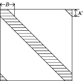
Then we adopt the Viterbi algorithm [20] to minimize (37). The frequency domain signal 𝐱~~𝐱\mathbf{\tilde{x}} is treated as a sequence of data and the correlation between data is determined by the ICI. Strictly speaking, for DSC, all the elements of 𝐃[𝐦~μ]𝐃delimited-[]subscript~𝐦𝜇\mathbf{D}[\mathbf{\tilde{m}}_{\mu}] and 𝐃[𝝃j]𝐃delimited-[]subscript𝝃𝑗\mathbf{D}[\boldsymbol{\xi}_{j}], j=1,,M𝑗1𝑀j=1,\ldots,M are nonzero. But the entries close to the main diagonal are more prominent compared to those further away from the diagonal. This means that, the matrices 𝐃[𝐦~μ]𝐃delimited-[]subscript~𝐦𝜇\mathbf{D}[\mathbf{\tilde{m}}_{\mu}] and 𝐃[𝝃j]𝐃delimited-[]subscript𝝃𝑗\mathbf{D}[\boldsymbol{\xi}_{j}] can be approximated as a banded matrix of bandwidth B=2κ+1𝐵2𝜅1B=2\kappa+1, as shown in Figure 2. This approximated banded structure of DSC matrix considers the most significant ICI from the left and right κ𝜅\kappa closest symbols, and has been widely used in the literature [6, 20]. As shown in Figure 2, the upper right and lower left nonzero entries of the matrix cause cyclic interference between the first and last subcarriers, making the problem different from the uni-directional convolutional code decoding, where Viterbi algorithm is commonly used. In order to avoid the complication, we set the first and last κ𝜅\kappa symbols to be zero.

With the banded structure of 𝐃[𝐦~μ]𝐃delimited-[]subscript~𝐦𝜇\mathbf{D}[\mathbf{\tilde{m}}_{\mu}] and 𝐃[𝝃j]𝐃delimited-[]subscript𝝃𝑗\mathbf{D}[\boldsymbol{\xi}_{j}], the branch metric becomes

𝒱B([𝐱~]n2κ:n;y(nκ))subscript𝒱𝐵subscriptdelimited-[]~𝐱:𝑛2𝜅𝑛𝑦𝑛𝜅\displaystyle\mathcal{V}_{B}([\mathbf{\tilde{x}}]_{n-2\kappa:n};y(n-\kappa)) =\displaystyle= ([𝐃[𝐦~μ]]n,nκ:n2κ[𝐱~]n2κ:n)H([𝐃[𝐦~μ]]n,nκ:n2κ[𝐱~]n2κ:n)superscriptsubscriptdelimited-[]𝐃delimited-[]subscript~𝐦𝜇:𝑛𝑛𝜅𝑛2𝜅subscriptdelimited-[]~𝐱:𝑛2𝜅𝑛𝐻subscriptdelimited-[]𝐃delimited-[]subscript~𝐦𝜇:𝑛𝑛𝜅𝑛2𝜅subscriptdelimited-[]~𝐱:𝑛2𝜅𝑛\displaystyle([\mathbf{D}[\mathbf{\tilde{m}}_{\mu}]]_{n,n-\kappa:n-2\kappa}[\mathbf{\tilde{x}}]_{n-2\kappa:n})^{H}([\mathbf{D}[\mathbf{\tilde{m}}_{\mu}]]_{n,n-\kappa:n-2\kappa}[\mathbf{\tilde{x}}]_{n-2\kappa:n}) (38)
+j=1Mλj([𝐃[𝝃j]]n,nκ:n2κ[𝐱~]n2κ:n)H([𝐃[𝝃j]]n,nκ:n2κ[𝐱~]n2κ:n)superscriptsubscript𝑗1𝑀subscript𝜆𝑗superscriptsubscriptdelimited-[]𝐃delimited-[]subscript𝝃𝑗:𝑛𝑛𝜅𝑛2𝜅subscriptdelimited-[]~𝐱:𝑛2𝜅𝑛𝐻subscriptdelimited-[]𝐃delimited-[]subscript𝝃𝑗:𝑛𝑛𝜅𝑛2𝜅subscriptdelimited-[]~𝐱:𝑛2𝜅𝑛\displaystyle+\sum_{j=1}^{M}\lambda_{j}([\mathbf{D}[\boldsymbol{\boldsymbol{\xi}}_{j}]]_{n,n-\kappa:n-2\kappa}[\mathbf{\tilde{x}}]_{n-2\kappa:n})^{H}([\mathbf{D}[\boldsymbol{\boldsymbol{\xi}}_{j}]]_{n,n-\kappa:n-2\kappa}[\mathbf{\tilde{x}}]_{n-2\kappa:n})
2Re{y(nκ)[𝐃[𝐦~μ]]n,nκ:n2κ[𝐱~]n2κ:n}.2Resuperscript𝑦𝑛𝜅subscriptdelimited-[]𝐃delimited-[]subscript~𝐦𝜇:𝑛𝑛𝜅𝑛2𝜅subscriptdelimited-[]~𝐱:𝑛2𝜅𝑛\displaystyle-2\mathrm{Re}\{{y}^{*}(n-{\kappa})[\mathbf{D}[\mathbf{\tilde{m}}_{\mu}]]_{n,n-\kappa:n-2\kappa}[\mathbf{\tilde{x}}]_{n-2\kappa:n}\}.

Since known pilot symbols are inserted between unknown data, slight modification to standard Viterbi algorithm is needed. For np𝑛subscript𝑝n\in\mathfrak{I}_{p}, the true pilot value will be used to calculate the branch value, and the number of remaining paths will reduce by half because of merging. And for nd𝑛subscript𝑑n\in\mathfrak{I}_{d}, the algorithm will perform as normal Viterbi algorithm.

IV-C2 Minimization w.r.t. 𝐦~μ,𝚺~μ,a~j,b~j,c~subscript~𝐦𝜇subscript~𝚺𝜇subscript~𝑎𝑗subscript~𝑏𝑗~𝑐\mathbf{\tilde{m}}_{\mu},\mathbf{\tilde{\Sigma}}_{\mu},\tilde{a}_{j},\tilde{b}_{j},\tilde{c} and d~~𝑑\tilde{d}

The optimal values of other unknown parameters are obtained by setting the first order derivative of (31) with respect to the corresponding parameter to zero. As shown in Appendix B, we obtain the following set of solutions:

𝚺~μsubscript~𝚺𝜇\displaystyle\mathbf{\tilde{\Sigma}}_{\mu} =\displaystyle= (diag{[a~1b~1,,a~Mb~M]}+c~d~𝐆H[𝐱~]𝐆[𝐱~])1superscriptdiagsubscript~𝑎1subscript~𝑏1subscript~𝑎𝑀subscript~𝑏𝑀~𝑐~𝑑superscript𝐆𝐻delimited-[]~𝐱𝐆delimited-[]~𝐱1\displaystyle\left(\mathrm{diag}\left\{\left[\frac{\tilde{a}_{1}}{\tilde{b}_{1}},\ldots,\frac{\tilde{a}_{M}}{\tilde{b}_{M}}\right]\right\}+\frac{\tilde{c}}{\tilde{d}}\mathbf{G}^{H}[\mathbf{\tilde{x}}]\mathbf{G}[\mathbf{\tilde{x}}]\right)^{-1} (39)
𝐦~μsubscript~𝐦𝜇\displaystyle\mathbf{\tilde{m}}_{\mu} =\displaystyle= c~d~𝚺~μ𝐆H[𝐱~]𝐲~𝑐~𝑑subscript~𝚺𝜇superscript𝐆𝐻delimited-[]~𝐱𝐲\displaystyle\frac{\tilde{c}}{\tilde{d}}\mathbf{\tilde{\Sigma}}_{\mu}\mathbf{G}^{H}[\mathbf{\tilde{x}}]\mathbf{y} (40)
a~jsubscript~𝑎𝑗\displaystyle\tilde{a}_{j} =\displaystyle= aj+1subscript𝑎𝑗1\displaystyle a_{j}+1 (41)
b~jsubscript~𝑏𝑗\displaystyle\tilde{b}_{j} =\displaystyle= bj+|[𝐦~μ]j|2+[𝚺~μ]j,jsubscript𝑏𝑗superscriptsubscriptdelimited-[]subscript~𝐦𝜇𝑗2subscriptdelimited-[]subscript~𝚺𝜇𝑗𝑗\displaystyle b_{j}+|[\mathbf{\tilde{m}}_{\mu}]_{j}|^{2}+[\mathbf{\tilde{\Sigma}}_{\mu}]_{j,j} (42)
c~~𝑐\displaystyle\tilde{c} =\displaystyle= c+N𝑐𝑁\displaystyle c+N (43)
d~~𝑑\displaystyle\tilde{d} =\displaystyle= d+𝐲H𝐲2Re{𝐲H𝐆[𝐱~]𝐦~μ}+Tr{𝐆H[𝐱~]𝐆[𝐱~](𝐦~μ𝐦~μH+𝚺~μ)}.𝑑superscript𝐲𝐻𝐲2Resuperscript𝐲𝐻𝐆delimited-[]~𝐱subscript~𝐦𝜇Trsuperscript𝐆𝐻delimited-[]~𝐱𝐆delimited-[]~𝐱subscript~𝐦𝜇superscriptsubscript~𝐦𝜇𝐻subscript~𝚺𝜇\displaystyle d+\mathbf{y}^{H}\mathbf{y}-2\mathrm{Re}\left\{\mathbf{y}^{H}\mathbf{G}\mathbf{[\tilde{x}]\tilde{m}}_{\mu}\right\}+\mathrm{Tr}\left\{\mathbf{G}^{H}[\mathbf{\tilde{x}}]\mathbf{G}[\mathbf{\tilde{x}}]\left(\mathbf{\tilde{m}}_{\mu}\mathbf{\tilde{m}}_{\mu}^{H}+\mathbf{\tilde{\Sigma}}_{\mu}\right)\right\}. (44)

It is worth noting that, along with each update, when |[𝐦~μ]j|2+[𝚺~μ]j,jsuperscriptsubscriptdelimited-[]subscript~𝐦𝜇𝑗2subscriptdelimited-[]subscript~𝚺𝜇𝑗𝑗|[\mathbf{\tilde{m}}_{\mu}]_{j}|^{2}+[\mathbf{\tilde{\Sigma}}_{\mu}]_{j,j} gets close to zero, meaning both mean and variance of the corresponding μjsubscript𝜇𝑗{\mu_{j}} are close to zero, then μjsubscript𝜇𝑗{\mu_{j}} can be treated as null entry and pruned from further iteration. In practice, a threshold with the order of 1010superscript101010^{-10} is used to compare with |[𝐦~μ]j|2+[𝚺~μ]j,jsuperscriptsubscriptdelimited-[]subscript~𝐦𝜇𝑗2subscriptdelimited-[]subscript~𝚺𝜇𝑗𝑗|[\mathbf{\tilde{m}}_{\mu}]_{j}|^{2}+[\mathbf{\tilde{\Sigma}}_{\mu}]_{j,j} to determine which μjsubscript𝜇𝑗{\mu_{j}} is being pruned [21].

IV-D Summary of the Iterative Algorithm

We summarize the parameter updating procedure as follows
Initialization: Choose initial values {a~10,,a~M0}superscriptsubscript~𝑎10superscriptsubscript~𝑎𝑀0\{\tilde{a}_{1}^{0},\ldots,\tilde{a}_{M}^{0}\}, {b~10,,b~M0}superscriptsubscript~𝑏10superscriptsubscript~𝑏𝑀0\{\tilde{b}_{1}^{0},\ldots,\tilde{b}_{M}^{0}\}, c~0,d~0superscript~𝑐0superscript~𝑑0\tilde{c}^{0},\tilde{d}^{0} and 𝐱~d0superscriptsubscript~𝐱𝑑0\mathbf{\tilde{x}}_{d}^{0}.
Iterations: For the ithsuperscript𝑖𝑡i^{th} iteration
Updating the parameters of GCE-BEM coefficients

𝚺~μisuperscriptsubscript~𝚺𝜇𝑖\displaystyle\mathbf{\tilde{\Sigma}}_{\mu}^{i} =\displaystyle= (diag{[a~1i1b~1i1,,a~Mi1b~Mi1]}+c~i1d~i1𝐆H[𝐱~i1]𝐆[𝐱~i1])1superscriptdiagsuperscriptsubscript~𝑎1𝑖1superscriptsubscript~𝑏1𝑖1superscriptsubscript~𝑎𝑀𝑖1superscriptsubscript~𝑏𝑀𝑖1superscript~𝑐𝑖1superscript~𝑑𝑖1superscript𝐆𝐻delimited-[]superscript~𝐱𝑖1𝐆delimited-[]superscript~𝐱𝑖11\displaystyle\Big{(}\mathrm{diag}\big{\{}\big{[}\frac{\tilde{a}_{1}^{i-1}}{\tilde{b}_{1}^{i-1}},\ldots,\frac{\tilde{a}_{M}^{i-1}}{\tilde{b}_{M}^{i-1}}\big{]}\big{\}}+\frac{\tilde{c}^{i-1}}{\tilde{d}^{i-1}}\mathbf{G}^{H}[\mathbf{\tilde{x}}^{i-1}]\mathbf{G}[\mathbf{\tilde{x}}^{i-1}]\Big{)}^{-1}
𝐦~μisuperscriptsubscript~𝐦𝜇𝑖\displaystyle\mathbf{\tilde{m}}_{\mu}^{i} =\displaystyle= c~i1d~i1𝚺~μi𝐆H[𝐱~i1]𝐲superscript~𝑐𝑖1superscript~𝑑𝑖1superscriptsubscript~𝚺𝜇𝑖superscript𝐆𝐻delimited-[]superscript~𝐱𝑖1𝐲\displaystyle\frac{\tilde{c}^{i-1}}{\tilde{d}^{i-1}}\mathbf{\tilde{\Sigma}}_{\mu}^{i}\mathbf{G}^{H}[\mathbf{\tilde{x}}^{i-1}]\mathbf{y}

Updating the hyperparameters of GCE-BEM coefficients

a~jisuperscriptsubscript~𝑎𝑗𝑖\displaystyle\tilde{a}_{j}^{i} =\displaystyle= aj+1subscript𝑎𝑗1\displaystyle a_{j}+1
b~jisuperscriptsubscript~𝑏𝑗𝑖\displaystyle\tilde{b}_{j}^{i} =\displaystyle= bj+|[𝐦~μ]j|2+[𝚺~μ]j,jsubscript𝑏𝑗superscriptsubscriptdelimited-[]subscript~𝐦𝜇𝑗2subscriptdelimited-[]subscript~𝚺𝜇𝑗𝑗\displaystyle b_{j}+|[\mathbf{\tilde{m}}_{\mu}]_{j}|^{2}+[\mathbf{\tilde{\Sigma}}_{\mu}]_{j,j}

Updating the estimate of data

min𝐱~d𝔽x~d=2Re{𝐲H𝐃[𝐦~μ]𝐱~}+𝐱~H𝐃H[𝐦~μ]𝐃[𝐦~μ]𝐱~+j=1Mλj𝐱~H𝐃H[𝝃j]𝐃[𝝃j]𝐱~,subscriptsubscript~𝐱𝑑subscript𝔽subscript~𝑥𝑑2Resuperscript𝐲𝐻𝐃delimited-[]subscript~𝐦𝜇~𝐱superscript~𝐱𝐻superscript𝐃𝐻delimited-[]subscript~𝐦𝜇𝐃delimited-[]subscript~𝐦𝜇~𝐱superscriptsubscript𝑗1𝑀subscript𝜆𝑗superscript~𝐱𝐻superscript𝐃𝐻delimited-[]subscript𝝃𝑗𝐃delimited-[]subscript𝝃𝑗~𝐱\begin{split}\min_{\mathbf{\tilde{x}}_{d}}\mathbb{F}_{\tilde{x}_{d}}=&-2\mathrm{Re}\left\{\mathbf{y}^{H}\mathbf{D}[\mathbf{\tilde{m}}_{\mu}]\mathbf{\tilde{x}}\right\}+\mathbf{\tilde{x}}^{H}\mathbf{D}^{H}[\mathbf{\tilde{m}}_{\mu}]\mathbf{D}[\mathbf{\tilde{m}}_{\mu}]\mathbf{\tilde{x}}+\sum_{j=1}^{M}\lambda_{j}\mathbf{\tilde{x}}^{H}\mathbf{D}^{H}[\boldsymbol{\boldsymbol{\xi}}_{j}]\mathbf{D}[\boldsymbol{\boldsymbol{\xi}}_{j}]\mathbf{\tilde{x}},\end{split}

where 𝚺~μi=j=1Mi1λji𝝃ji(𝝃ji)Hsuperscriptsubscript~𝚺𝜇𝑖superscriptsubscript𝑗1superscript𝑀𝑖1superscriptsubscript𝜆𝑗𝑖superscriptsubscript𝝃𝑗𝑖superscriptsuperscriptsubscript𝝃𝑗𝑖𝐻\mathbf{\tilde{\Sigma}}_{\mu}^{i}=\sum_{j=1}^{M^{i-1}}\lambda_{j}^{i}\mathbf{\boldsymbol{\xi}}_{j}^{i}(\mathbf{\boldsymbol{\xi}}_{j}^{i})^{H}, using Viterbi algorithm.
Updating the hyperparameters of noise

c~isuperscript~𝑐𝑖\displaystyle\tilde{c}^{i} =\displaystyle= c+N𝑐𝑁\displaystyle c+N
d~isuperscript~𝑑𝑖\displaystyle\tilde{d}^{i} =\displaystyle= d+𝐲H𝐲2Re{𝐲H𝐆[𝐱~i]𝐦~μi}+Tr{𝐆H[𝐱~i]𝐆[𝐱~i](𝐦~μi(𝐦~μi)H+𝚺~μi)}𝑑superscript𝐲𝐻𝐲2Resuperscript𝐲𝐻𝐆delimited-[]superscript~𝐱𝑖superscriptsubscript~𝐦𝜇𝑖Trsuperscript𝐆𝐻delimited-[]superscript~𝐱𝑖𝐆delimited-[]superscript~𝐱𝑖superscriptsubscript~𝐦𝜇𝑖superscriptsuperscriptsubscript~𝐦𝜇𝑖𝐻superscriptsubscript~𝚺𝜇𝑖\displaystyle d+\mathbf{y}^{H}\mathbf{y}-2\mathrm{Re}\left\{\mathbf{y}^{H}\mathbf{G}\mathbf{[\tilde{x}}^{i}]\mathbf{\tilde{m}}_{\mu}^{i}\right\}+\mathrm{Tr}\left\{\mathbf{G}^{H}[\mathbf{\tilde{x}}^{i}]\mathbf{G}[\mathbf{\tilde{x}}^{i}]\left(\mathbf{\tilde{m}}_{\mu}^{i}(\mathbf{\tilde{m}}_{\mu}^{i})^{H}+\mathbf{\tilde{\Sigma}}_{\mu}^{i}\right)\right\}

Pruning
If |[𝐦~μ]j|2+[𝚺~μ]j,j<1010μj=0superscriptsubscriptdelimited-[]subscript~𝐦𝜇𝑗2subscriptdelimited-[]subscript~𝚺𝜇𝑗𝑗superscript1010subscript𝜇𝑗0|[\mathbf{\tilde{m}}_{\mu}]_{j}|^{2}+[\mathbf{\tilde{\Sigma}}_{\mu}]_{j,j}<10^{-10}\Rightarrow{\mu_{j}}=0, remove a~jsubscript~𝑎𝑗\tilde{a}_{j} from {a~1i,,a~Mi}superscriptsubscript~𝑎1𝑖superscriptsubscript~𝑎𝑀𝑖\{\tilde{a}_{1}^{i},\ldots,\tilde{a}_{M}^{i}\} and b~jsubscript~𝑏𝑗\tilde{b}_{j} from {b~1i,,b~Mi}superscriptsubscript~𝑏1𝑖superscriptsubscript~𝑏𝑀𝑖\{\tilde{b}_{1}^{i},\ldots,\tilde{b}_{M}^{i}\} and update the expression of 𝐆[𝐱~i]𝐆delimited-[]superscript~𝐱𝑖\mathbf{G[\tilde{x}}^{i}] by removing the jthsuperscript𝑗𝑡j^{th} column.
End
It is worth noting that the values of {a~1,,a~M}subscript~𝑎1subscript~𝑎𝑀\{\tilde{a}_{1},\ldots,\tilde{a}_{M}\} and c~~𝑐\tilde{c} remain the same for each iteration, thus they should only be updated in the first iteration in practice.

V Initialization of the Iterative Algorithm

In order to start the iteration, one of the quantities we need is the initial data estimate 𝐱~d0superscriptsubscript~𝐱𝑑0\mathbf{\tilde{x}}_{d}^{0}. If an initial channel estimate can be obtained from pilots, then from (19), the initial data estimate can be obtained. In Section III, GCE-BEM with large oversampling factor is used to represent the channel. Though this provides flexibility for selecting important bases in the iterative channel estimation and data detection, the large number of unknown coefficients corresponding to GCE-BEM also brings challenges in the initial value estimation, which is important to any iterative algorithm. Unfortunately, traditional compressed sensing methods like BP and orthogonal matching pursuit (OMP), whose performance highly depends on the accurate knowledge of noise variance, is not applicable in our case, since the variance of the composite noise is unknown.

On the other hand, notice that the proposed iterative algorithm does not rely directly on the estimate of 𝝁𝝁{\boldsymbol{\mu}} to start the iteration. The channel is needed only indirectly through initial data estimate. Thus, during initial data detection, we choose to expand the channel with CE-BEM, which corresponds to choosing the oversampling factor of GCE-BEM as V=1𝑉1V=1. Then least squares (LS) algorithm is used to obtain the initial channel estimation. Though CE-BEM is widely reported as relatively inaccurate among other BEMs, it represents the time-varying channel using a very small number of orthogonal bases. This is highly beneficial for a rough estimate at the initial stage where there is little knowledge of the channel and source signal at the receiver.

According to (2), 𝐱=𝐄d𝐱d+𝐄p𝐱p𝐱subscript𝐄𝑑subscript𝐱𝑑subscript𝐄𝑝subscript𝐱𝑝\mathbf{x=E}_{d}\mathbf{x}_{d}+\mathbf{E}_{p}\mathbf{x}_{p}. Together with the fact that 𝐆[𝐄p𝐱p+𝐄d𝐱d]=𝐆[𝐄p𝐱p]+𝐆[𝐄d𝐱d]𝐆delimited-[]subscript𝐄𝑝subscript𝐱𝑝subscript𝐄𝑑subscript𝐱𝑑𝐆delimited-[]subscript𝐄𝑝subscript𝐱𝑝𝐆delimited-[]subscript𝐄𝑑subscript𝐱𝑑\mathbf{G[E}_{p}\mathbf{x}_{p}+\mathbf{E}_{d}\mathbf{x}_{d}]=\mathbf{G[E}_{p}\mathbf{x}_{p}]+\mathbf{G[E}_{d}\mathbf{x}_{d}], (18) can be written as 𝐲=𝐆[𝐄p𝐱p]𝝁+𝐆[𝐄d𝐱d]𝝁+𝐯𝐲𝐆delimited-[]subscript𝐄𝑝subscript𝐱𝑝𝝁𝐆delimited-[]subscript𝐄𝑑subscript𝐱𝑑𝝁𝐯\mathbf{y}=\mathbf{G[E}_{p}\mathbf{x}_{p}]{\boldsymbol{\mu}}+\mathbf{G[E}_{d}\mathbf{x}_{d}]{\boldsymbol{\mu}}+\mathbf{v}. Collecting the output samples corresponding to pilot positions psubscript𝑝\mathfrak{I}_{p}, the equation for initial channel estimation can be written as

𝐲p=𝐆p[𝐄p𝐱p]𝝁+𝐆p[𝐄d𝐱d]𝝁+𝐯p,subscript𝐲𝑝subscript𝐆𝑝delimited-[]subscript𝐄𝑝subscript𝐱𝑝𝝁subscript𝐆𝑝delimited-[]subscript𝐄𝑑subscript𝐱𝑑𝝁subscript𝐯𝑝\mathbf{y}_{p}=\mathbf{G}_{p}\mathbf{[E}_{p}\mathbf{x}_{p}]{\boldsymbol{\mu}}+\mathbf{G}_{p}\mathbf{[E}_{d}\mathbf{x}_{d}]{\boldsymbol{\mu}}\mathbf{+v}_{p}, (45)

where 𝐆p[.]\mathbf{G}_{p}[.] is constructed from the rows of 𝐆[.]\mathbf{G}[.] corresponding to psubscript𝑝\mathfrak{I}_{p}. The initial channel estimation can be obtained by treating the second term of (45) as noise and performing LS algorithm:

𝝁^=(𝐆pH[𝐄p𝐱p]𝐆p[𝐄p𝐱p])1𝐆pH[𝐄p𝐱p]𝐲p.^𝝁superscriptsuperscriptsubscript𝐆𝑝𝐻delimited-[]subscript𝐄𝑝subscript𝐱𝑝subscript𝐆𝑝delimited-[]subscript𝐄𝑝subscript𝐱𝑝1subscriptsuperscript𝐆𝐻𝑝delimited-[]subscript𝐄𝑝subscript𝐱𝑝subscript𝐲𝑝\hat{{\boldsymbol{\mu}}}=(\mathbf{G}_{p}^{H}\mathbf{[E}_{p}\mathbf{x}_{p}]\mathbf{G}_{p}\mathbf{[E}_{p}\mathbf{x}_{p}])^{-1}\mathbf{G}^{H}_{p}\mathbf{[E}_{p}\mathbf{x}_{p}]\mathbf{y}_{p}. (46)

With the estimated channel 𝝁^^𝝁\hat{{\boldsymbol{\mu}}}, we rewrite (19) as 𝐲=𝐃[𝝁^]𝐄d𝐱d+𝐃[𝝁^]𝐄p𝐱p+𝐯.𝐲𝐃delimited-[]^𝝁subscript𝐄𝑑subscript𝐱𝑑𝐃delimited-[]^𝝁subscript𝐄𝑝subscript𝐱𝑝𝐯\mathbf{y=D[\hat{{\boldsymbol{\mu}}}]E}_{d}\mathbf{x}_{d}+\mathbf{D[\hat{{\boldsymbol{\mu}}}]E}_{p}\mathbf{x}_{p}+\mathbf{v}. Applying LS estimation again, we have

𝐱^d0=(𝐄dH𝐃H[𝝁^]𝐃[𝝁^]𝐄d)1𝐄dH𝐃H[𝝁^](𝐲𝐃[𝝁^]𝐄p𝐱p).superscriptsubscript^𝐱𝑑0superscriptsuperscriptsubscript𝐄𝑑𝐻superscript𝐃𝐻delimited-[]^𝝁𝐃delimited-[]^𝝁subscript𝐄𝑑1superscriptsubscript𝐄𝑑𝐻superscript𝐃𝐻delimited-[]^𝝁𝐲𝐃delimited-[]^𝝁subscript𝐄𝑝subscript𝐱𝑝\mathbf{\hat{x}}_{d}^{0}=(\mathbf{E}_{d}^{H}\mathbf{D}^{H}[\hat{{\boldsymbol{\mu}}}]\mathbf{D}[\hat{{\boldsymbol{\mu}}}]\mathbf{E}_{d})^{-1}\mathbf{E}_{d}^{H}\mathbf{D}^{H}[\hat{{\boldsymbol{\mu}}}](\mathbf{y}-\mathbf{D[\hat{{\boldsymbol{\mu}}}]E}_{p}\mathbf{x}_{p}). (47)

The obtained 𝐱^d0superscriptsubscript^𝐱𝑑0\mathbf{\hat{x}}_{d}^{0} may not reside on the constellation map, thus quantization is performed on 𝐱^d0superscriptsubscript^𝐱𝑑0\mathbf{\hat{x}}_{d}^{0} and the initial data detection is given as 𝐱~d0=Qant[𝐱^d0]superscriptsubscript~𝐱𝑑0Qantdelimited-[]superscriptsubscript^𝐱𝑑0\mathbf{\tilde{x}}_{d}^{0}=\mathrm{Qant}[\mathbf{\hat{x}}_{d}^{0}]. Notice that in DSC, the ICI is not negligible, and 𝐆p[𝐄d𝐱d]𝝁𝟎subscript𝐆𝑝delimited-[]subscript𝐄𝑑subscript𝐱𝑑𝝁0\mathbf{G}_{p}\mathbf{[E}_{d}\mathbf{x}_{d}]{\boldsymbol{\mu}}\neq\mathbf{0}, which decreases the accuracy of estimation in (46), and in turns affects the accuracy of initial data detection. This is the reason why an iterative algorithm is necessary.

For other initial values {a~10,,a~M0}superscriptsubscript~𝑎10superscriptsubscript~𝑎𝑀0\{\tilde{a}_{1}^{0},\ldots,\tilde{a}_{M}^{0}\}, {b~10,,b~M0}superscriptsubscript~𝑏10superscriptsubscript~𝑏𝑀0\{\tilde{b}_{1}^{0},\ldots,\tilde{b}_{M}^{0}\}, c~0,d~0superscript~𝑐0superscript~𝑑0\tilde{c}^{0},\tilde{d}^{0} in the iterative algorithm, it is should be noticed that only the ratios a~j/b~jsubscript~𝑎𝑗subscript~𝑏𝑗\tilde{a}_{j}/\tilde{b}_{j} and c~/d~~𝑐~𝑑\tilde{c}/\tilde{d} are required, thus we only need to specify the initial values of the ratios to start the iteration. From (28) and the property of Gamma distribution, a~j/b~jsubscript~𝑎𝑗subscript~𝑏𝑗\tilde{a}_{j}/\tilde{b}_{j} represents the mean value of αjsubscript𝛼𝑗\alpha_{j}, which is the inverse variance of channel GCE-BEM coefficients. Since we have no information about their relative values, we can set them to be equal. That is, let a~j0/b~j0=1/Msuperscriptsubscript~𝑎𝑗0superscriptsubscript~𝑏𝑗01𝑀\tilde{a}_{j}^{0}/\tilde{b}_{j}^{0}=1/M for all j𝑗j. Furthermore, from (29) and the property of Gamma distribution, c~/d~=𝔼{β}=𝔼{1/ϖv2}~𝑐~𝑑𝔼𝛽𝔼1superscriptsubscriptitalic-ϖ𝑣2\tilde{c}/\tilde{d}=\mathbb{E}\{\beta\}=\mathbb{E}\{1/\varpi_{v}^{2}\}. Therefore the initial value can be set as c~0/d~0=1/ϖ^v2superscript~𝑐0superscript~𝑑01superscriptsubscript^italic-ϖ𝑣2{\tilde{c}^{0}}/{\tilde{d}^{0}}={1}/{\hat{\varpi}_{v}^{2}}, where ϖ^v2superscriptsubscript^italic-ϖ𝑣2\hat{\varpi}_{v}^{2} is an estimate of noise power

ϖ^v2=𝐲𝐆[𝐄p𝐱p+𝐄d𝐱~d0]𝝁^.superscriptsubscript^italic-ϖ𝑣2𝐲𝐆delimited-[]subscript𝐄𝑝subscript𝐱𝑝subscript𝐄𝑑superscriptsubscript~𝐱𝑑0^𝝁\hat{\varpi}_{v}^{2}=\mathbf{y-G[E}_{p}\mathbf{x}_{p}+\mathbf{E}_{d}\mathbf{\tilde{x}}_{d}^{0}]\hat{{\boldsymbol{\mu}}}. (48)

VI Simulation Results and Discussions

In this section, simulation results of dual-hop and three-hop cooperative OFDM systems are provided. In both systems, each OFDM symbol has 128 subcarriers and the length of CP is 8. Carrier frequency is fc=2subscript𝑓𝑐2f_{c}=2GHz and the sample interval is Ts=2μssubscript𝑇𝑠2𝜇𝑠T_{s}=2\mu s. The channel h¯k,ρ(n,l)subscript¯𝑘𝜌𝑛𝑙\bar{h}_{k,\rho}(n,l) is generated according to zero-mean complex Gaussian distribution with autocorrelation of the lthsuperscript𝑙𝑡l^{th} tap given by 𝔼{h¯k,ρ(m,l)h¯k,ρ(n,l)}=σk,ρ2(l)J0(2πfk,ρ(l)(mn)Ts)𝔼subscript¯𝑘𝜌𝑚𝑙subscript¯𝑘𝜌𝑛𝑙superscriptsubscript𝜎𝑘𝜌2𝑙subscript𝐽02𝜋subscript𝑓𝑘𝜌𝑙𝑚𝑛subscript𝑇𝑠\mathbb{E}\{\bar{h}_{k,\rho}(m,l)\bar{h}_{k,\rho}(n,l)\}=\sigma_{k,\rho}^{2}(l)J_{0}(2\pi f_{k,\rho}(l)(m-n)T_{s}) [22], where J0()subscript𝐽0J_{0}(\cdot) represents the zero-order Bessel function of the first kind, and σk,ρ2(l)superscriptsubscript𝜎𝑘𝜌2𝑙\sigma_{k,\rho}^{2}(l) is the power of the lthsuperscript𝑙𝑡l^{th} tap. Fourteen pilot clusters are used. The clusters are equal-spaced and interleaved with data subcarriers. In each cluster, one nonzero pilot is guarded by one zero pilot on each side. The nonzero pilots are generated as zero-mean complex Gaussian random variables with power three times that of data symbols. And the data is modulated with QPSK of unit power. The normalized channel mean-square error (MSE) and data detection bit error rate (BER) are plotted to demonstrate the performance. The MSE of the channel estimate at the ithsuperscript𝑖𝑡i^{th} iteration is defined as MSEi=𝐇^i𝐇2/𝐇2superscriptMSE𝑖superscriptnormsuperscript^𝐇𝑖𝐇2superscriptnorm𝐇2\mathrm{MSE}^{i}={\|\mathbf{\hat{H}}^{i}-\mathbf{H}\|^{2}}/{\|\mathbf{H}\|^{2}}, where 𝐇^isuperscript^𝐇𝑖\mathbf{\hat{H}}^{i} is the channel matrix recovered from the GCE-BEM estimate at the ithsuperscript𝑖𝑡i^{th} iteration. The noise power at the relays and destination are set to be the same ϖd2=ϖk,ρ2,superscriptsubscriptitalic-ϖ𝑑2superscriptsubscriptitalic-ϖ𝑘𝜌2\varpi_{d}^{2}=\varpi_{k,\rho}^{2}, for all k𝑘k and ρ𝜌\rho. The signal-to-noise ratio (SNR) in the following figures is defined as SNR=σs2/ϖd2SNRsuperscriptsubscript𝜎𝑠2superscriptsubscriptitalic-ϖ𝑑2\mathrm{SNR}=\sigma_{s}^{2}/\varpi_{d}^{2} [9]. The oversampling factor is chosen as V=20𝑉20V=20 for GCE-BEM. Each point is obtained by averaging the results over 1,000 runs.

For the dual-hop system, two relaying paths (K𝐾K = 2) are considered. For both relaying paths (k=1,2𝑘12k=1,2), the maximal normalized Doppler shifts111Normalized Doppler shift is defined as NfdTs𝑁subscript𝑓𝑑subscript𝑇𝑠Nf_{d}T_{s} with fdsubscript𝑓𝑑f_{d} being the Doppler frequency. are set as 0.05 for the first hop and 0.15 for the second hop. In the simulation, for each specific channel, one randomly chosen tap has Doppler shift equals the maximum Doppler shift specified above. And for other taps, their Doppler shifts are uniformly drawn within the range from 0 to the maximum Doppler shift. Both source-relay channels have 2 taps. One of the source-relay channels has tap positions uniformly drawn from {0,1,2}012\{0,1,2\} while the other has tap positions uniformly drawn from {0,1,2,3,4}01234\{0,1,2,3,4\}. And both relay-destination channels have 2 taps, with the tap positions uniformly drawn from {0,1,2,3}0123\{0,1,2,3\} for one channel and from {0,1,2}012\{0,1,2\} for the other. All the channels follow exponential power delay profiles normalized to unit power. For the Viterbi equalizer, κ=3𝜅3\kappa=3 is chosen.

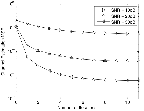
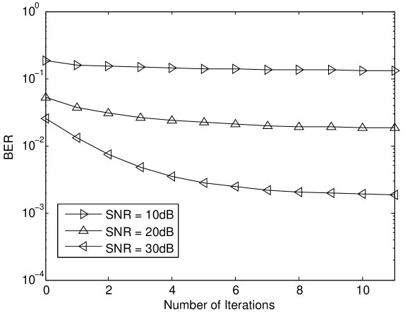
Figure 3 and Figure 4 present the convergence performance of the proposed iterative algorithm in terms of MSE and BER, respectively. SNR is set at 10dB, 20dB and 30dB. It can be seen that the MSEs and BERs improve significantly in the first few iterations and converge to stable values before 10 iterations.

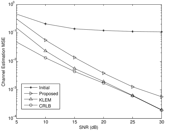
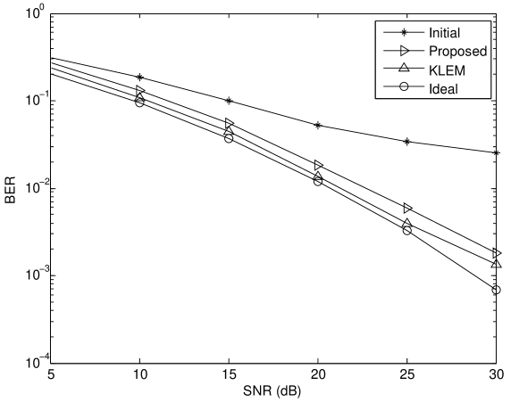
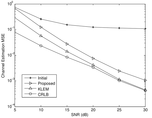
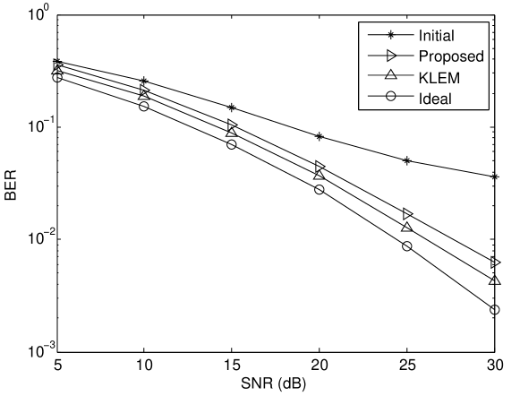
Figure 5 and Figure 6 show the MSE and BER performance achieved by the proposed iterative algorithm versus SNRs. The results are taken after 10 iterations in order to guarantee convergence. In the figures, KLEM represents the performance of the EM algorithm with channel expanded on Karhuen-Loève (KL) bases. This algorithm is an extension of the KLEM algorithm for single-hop case [23], and the detail is not included in this paper due to space limitation. The KLEM algorithm requires full information on channel tap positions, Doppler frequencies and power profile of each channel, together with noise statistics, thus serves as a reference for optimal performance here. And CRLB curve represents the Crame´´e\mathrm{\acute{e}}-Rao lower bound, which can be obtained from [23] by replacing the single-hop channel and noise power with the composite channel and composite noise power. Meanwhile, ideal case with full channel information at the receiver is also depicted as the performance bound in the BER figure. From Figure 5 and 6, it can be seen that, the proposed iterative algorithm successfully eliminates the interdependence between data detection and channel estimation, and exhibits significant performance improvement compared to the initial channel estimation MSE and data detection BER. Furthermore, though the proposed iterative algorithm does not have access to the relaying system structure (number of available links K𝐾K) or any statistical information of the channel and noise, there are only minor performance gaps between the proposed method and the KLEM. Furthermore, the proposed algorithm and KLEM are very close to the ideal data detection in terms of BER performance.

For three-hop relaying system, the maximal normalized Doppler shifts for the first and third hop are set as 0.05 while that of the second hop is set as 0.15. Two relaying paths are considered (K𝐾K= 2). For the first relaying path, the number of channel taps in the three hops are {2,3,2}232\{2,3,2\}, respectively; while that for the second relaying path is {3,2,2}322\{3,2,2\}, respectively. The channel taps in each hop are consecutive. For the Viterbi equalizer, κ=4𝜅4\kappa=4 is chosen.

Figure 7 and Figure 8 show the MSE and BER performance achieved by the proposed iterative algorithm versus SNRs, with results taken after 10 iterations222As the convergence performance of a three-hop system is similar to that of dual-hop system, the convergence figures are not shown here.. In both figures, performance curves of KLEM, which demands detailed information of relaying system structure, channel and noise statistics, are depicted as a reference for optimal channel estimation and data detection. From Figure 7, it is seen that, the proposed iterative algorithm greatly improve the performance from the initial channel estimation, indicating the ability of the proposed algorithm to cancel interference between unknown data and pilots through iterations. Furthermore, after convergence, only a small performance gap exists between the proposed algorithm and KLEM, which touches the CRLB at high SNRs. This exhibits the strong ability of our proposed algorithm in learning the statistics of both channel and noise. From Figure 8, the BER performance of our proposed method is also shown to improve significantly compared to the initial data detection and is very close that of KLEM algorithm. From these figures, it can be concluded that, though the system model in a three-hop system is more complicated than that of dual-hop case, the proposed algorithm continues to present good performance in terms of both channel estimation MSE and data detection BER and demonstrate robustness in a variety of OFDM relaying systems.

VII Conclusions

In this paper, channel estimation and data detection for multihop OFDM relaying system under high mobility has been investigated with focus on unknown channel orders and Doppler frequencies. By exploring the matrix structure of channels in different hops, we first simplified the multihop multilink channel matrix into a composite channel matrix. Then the composite channel was represented using GCE-BEM with a large oversampling factor so that sparsity on the delay-Doppler domain was introduced. Sparsity enhancing Gaussian priors with Gamma hyperpriors were adopted to enable the identification of nonzero entries. A pilot-aided iterative algorithm was developed under variational inference (VI) framework, using only limited number of pilot subcarriers in one OFDM symbol. The proposed algorithm iteratively estimates the channel, recovers the unknown data using Viterbi algorithm and learns the channel and noise statistical information. Simulation results showed that, even without any specific information on system structure, channel tap positions, channel lengths, Doppler shifts and noise powers, the proposed algorithms exhibited performance very close to that of an optimal channel estimation and data detection algorithm, which requires all of the above information.

Appendix A Calculation of Free Energy Function

Taking logarithm on (27) and substituting the result to the first term of (25), we obtain

𝝁Q(𝝁)logQ(𝝁)𝑑𝝁subscript𝝁𝑄𝝁𝑄𝝁differential-d𝝁\displaystyle\int_{{\boldsymbol{\mu}}}Q({\boldsymbol{\mu}})\log Q({\boldsymbol{\mu}})d{\boldsymbol{\mu}} =\displaystyle= Mlogπlogdet(𝚺~μ)𝐦~μH𝚺~μ1𝐦~μ𝑀𝜋subscript~𝚺𝜇superscriptsubscript~𝐦𝜇𝐻superscriptsubscript~𝚺𝜇1subscript~𝐦𝜇\displaystyle-M\log\pi-\log\det(\mathbf{\tilde{\Sigma}}_{\mu})-\mathbf{\tilde{m}}_{\mu}^{H}\mathbf{\tilde{\Sigma}}_{\mu}^{-1}\mathbf{\tilde{m}}_{\mu} (49)
+2Re{𝔼{𝝁H}𝚺~μ1𝐦~μ}Tr{𝚺~μ1𝔼{𝝁𝝁H}}2Re𝔼superscript𝝁𝐻superscriptsubscript~𝚺𝜇1subscript~𝐦𝜇Trsuperscriptsubscript~𝚺𝜇1𝔼𝝁superscript𝝁𝐻\displaystyle+2\mathrm{\mathrm{Re}}\left\{\mathbb{E}\{{\boldsymbol{\mu}}^{H}\}\mathbf{\tilde{\Sigma}}_{\mu}^{-1}\mathbf{\tilde{m}}_{\mu}\right\}-\mathrm{Tr}\left\{\mathbf{\tilde{\Sigma}}_{\mu}^{-1}\mathbb{E}\{\boldsymbol{\mu}\boldsymbol{\mu}^{H}\}\right\}
=\displaystyle= Mlogπlogdet(𝚺~μ)𝐦~μH𝚺~μ1𝐦~μ𝑀𝜋subscript~𝚺𝜇superscriptsubscript~𝐦𝜇𝐻superscriptsubscript~𝚺𝜇1subscript~𝐦𝜇\displaystyle-M\log\pi-\log\det(\mathbf{\tilde{\Sigma}}_{\mu})-\mathbf{\tilde{m}}_{\mu}^{H}\mathbf{\tilde{\Sigma}}_{\mu}^{-1}\mathbf{\tilde{m}}_{\mu}
+2𝐦~μH𝚺~μ1𝐦~μTr{𝚺~μ1(𝐦~μ𝐦~μH+𝚺~μ)}2superscriptsubscript~𝐦𝜇𝐻superscriptsubscript~𝚺𝜇1subscript~𝐦𝜇Trsuperscriptsubscript~𝚺𝜇1subscript~𝐦𝜇superscriptsubscript~𝐦𝜇𝐻subscript~𝚺𝜇\displaystyle+2\mathbf{\tilde{m}}_{\mu}^{H}\mathbf{\tilde{\Sigma}}_{\mu}^{-1}\mathbf{\tilde{m}}_{\mu}-\mathrm{Tr}\left\{\mathbf{\tilde{\Sigma}}_{\mu}^{-1}(\mathbf{\tilde{m}}_{\mu}\mathbf{\tilde{m}}_{\mu}^{H}+\mathbf{\tilde{\Sigma}}_{\mu})\right\}
=\displaystyle= Mlogπlogdet(𝚺~μ)M.𝑀𝜋subscript~𝚺𝜇𝑀\displaystyle-M\log\pi-\log\det(\mathbf{\tilde{\Sigma}}_{\mu})-M.

On the other hand, from the form of Q(αj)𝑄subscript𝛼𝑗Q(\alpha_{j}) given in (28), and notice that Q(𝜶)=j=1MQ(αj)𝑄𝜶superscriptsubscriptproduct𝑗1𝑀𝑄subscript𝛼𝑗Q(\boldsymbol{\alpha})=\prod_{j=1}^{M}Q(\alpha_{j}), we can compute the second term of (25) as

𝜶Q(𝜶)logQ(𝜶)𝑑𝜶subscript𝜶𝑄𝜶𝑄𝜶differential-d𝜶\displaystyle\int_{\boldsymbol{\alpha}}Q(\boldsymbol{\alpha})\log Q(\boldsymbol{\alpha})d\boldsymbol{\alpha} =\displaystyle= j=1M[a~jlogb~jlogΓ(a~j)+(a~j1)𝔼{logαj}b~j𝔼{αj}]superscriptsubscript𝑗1𝑀delimited-[]subscript~𝑎𝑗subscript~𝑏𝑗Γsubscript~𝑎𝑗subscript~𝑎𝑗1𝔼subscript𝛼𝑗subscript~𝑏𝑗𝔼subscript𝛼𝑗\displaystyle\sum_{j=1}^{M}\left[\tilde{a}_{j}\log\tilde{b}_{j}-\log\Gamma(\tilde{a}_{j})+(\tilde{a}_{j}-1)\mathbb{E}\{\log\alpha_{j}\}-\tilde{b}_{j}\mathbb{E}\{\alpha_{j}\}\right] (50)
=\displaystyle= j=1M[a~jlogb~jlogΓ(a~j)\displaystyle\sum_{j=1}^{M}\Big{[}\tilde{a}_{j}\log\tilde{b}_{j}-\log\Gamma(\tilde{a}_{j})
+(a~j1)(Ψ(a~j)logb~j)b~j(a~j/b~j)]\displaystyle+(\tilde{a}_{j}-1)\left(\Psi(\tilde{a}_{j})-\log\tilde{b}_{j}\right)-\tilde{b}_{j}\left({\tilde{a}_{j}}/{\tilde{b}_{j}}\right)\Big{]}
=\displaystyle= j=1M[logb~jlogΓ(a~j)+(a~j1)Ψ(a~j)a~j],superscriptsubscript𝑗1𝑀delimited-[]subscript~𝑏𝑗Γsubscript~𝑎𝑗subscript~𝑎𝑗1Ψsubscript~𝑎𝑗subscript~𝑎𝑗\displaystyle\sum_{j=1}^{M}\left[\log\tilde{b}_{j}-\log\Gamma(\tilde{a}_{j})+(\tilde{a}_{j}-1)\Psi(\tilde{a}_{j})-\tilde{a}_{j}\right],

where the digamma function ΨΨ\Psi is defined by Ψ(a)=alogΓ(a).Ψ𝑎𝑎Γ𝑎\displaystyle\Psi(a)=\frac{\partial}{\partial a}\log\Gamma(a). Furthermore, since Q(β)𝑄𝛽Q(\beta) is in the same form as Q(αj)𝑄subscript𝛼𝑗Q(\alpha_{j}), following a similar derivation as above, it can be easily shown that the third term of (25) is

βQ(β)logQ(β)𝑑β=logd~logΓ(c~)+(c~1)Ψ(c~)c~.subscript𝛽𝑄𝛽𝑄𝛽differential-d𝛽~𝑑Γ~𝑐~𝑐1Ψ~𝑐~𝑐\displaystyle\int_{\beta}Q(\beta)\log Q(\beta)d\beta=\log\tilde{d}-\log\Gamma(\tilde{c})+(\tilde{c}-1)\Psi(\tilde{c})-\tilde{c}. (51)

Based on the Dirac delta function in (30), the forth term of (25) is given by

𝐱dQ(𝐱d)logQ(𝐱d)𝑑𝐱dsubscriptsubscript𝐱𝑑𝑄subscript𝐱𝑑𝑄subscript𝐱𝑑differential-dsubscript𝐱𝑑\displaystyle\int_{\mathbf{x}_{d}}Q(\mathbf{x}_{d})\log Q(\mathbf{x}_{d})d\mathbf{x}_{d} =\displaystyle= logQ(𝐱~d)=logδ(𝐱~d𝐱~d)=0.𝑄subscript~𝐱𝑑𝛿subscript~𝐱𝑑subscript~𝐱𝑑0\displaystyle\log Q(\mathbf{\tilde{x}}_{d})=\log\delta(\mathbf{\tilde{x}}_{d}-\mathbf{\tilde{x}}_{d})=0. (52)

Furthermore, from (20), we have

logp(𝝁|𝜶)𝑝conditional𝝁𝜶\displaystyle\log p({\boldsymbol{\mu}}|\boldsymbol{\alpha}) =\displaystyle= Mlogπlogdet(𝐀1)𝝁H𝐀𝝁𝑀𝜋superscript𝐀1superscript𝝁𝐻𝐀𝝁\displaystyle-M\log\pi-\log\det(\mathbf{A}^{-1})-{\boldsymbol{\mu}}^{H}\mathbf{A}{\boldsymbol{\mu}} (53)
=\displaystyle= Mlogπ+log(j=1Mαj)Tr{𝐀𝝁𝝁H}.𝑀𝜋superscriptsubscriptproduct𝑗1𝑀subscript𝛼𝑗Tr𝐀𝝁superscript𝝁𝐻\displaystyle-M\log\pi+\log\left(\prod_{j=1}^{M}\alpha_{j}\right)-\mathrm{Tr}\left\{\mathbf{A}{\boldsymbol{\mu}}{\boldsymbol{\mu}}^{H}\right\}.

And the fifth term of (25) can be computed as

𝝁,𝜶Q(𝝁)Q(𝜶)logp(𝝁|𝜶)𝑑𝝁𝑑𝜶subscript𝝁𝜶𝑄𝝁𝑄𝜶𝑝conditional𝝁𝜶differential-d𝝁differential-d𝜶\displaystyle\int_{{\boldsymbol{\mu}},\boldsymbol{\alpha}}Q({\boldsymbol{\mu}})Q(\boldsymbol{\alpha})\log p({\boldsymbol{\mu}}|\boldsymbol{\alpha})d{\boldsymbol{\mu}}d\boldsymbol{\alpha} (54)
=\displaystyle= Mlogπ+j=1M𝔼α{logαj}Tr{𝔼α{diag{𝜶}}𝔼μ{𝝁𝝁H}}𝑀𝜋superscriptsubscript𝑗1𝑀subscript𝔼𝛼subscript𝛼𝑗Trsubscript𝔼𝛼diag𝜶subscript𝔼𝜇𝝁superscript𝝁𝐻\displaystyle-M\log\pi+\sum_{j=1}^{M}\mathbb{E}_{\alpha}\{\log\alpha_{j}\}-\mathrm{Tr}\{\mathbb{E}_{\alpha}\{\mathrm{diag}\{\boldsymbol{\alpha}\}\}\mathbb{E}_{\mu}\{{\boldsymbol{\mu}}{\boldsymbol{\mu}}^{H}\}\}
=\displaystyle= Mlogπ+j=1M(Ψ(a~j)logb~j)Tr{diag{[a~1b~1,,a~Mb~M]}(𝐦~μ𝐦~μH+𝚺~μ)}.𝑀𝜋superscriptsubscript𝑗1𝑀Ψsubscript~𝑎𝑗subscript~𝑏𝑗Trdiagsubscript~𝑎1subscript~𝑏1subscript~𝑎𝑀subscript~𝑏𝑀subscript~𝐦𝜇superscriptsubscript~𝐦𝜇𝐻subscript~𝚺𝜇\displaystyle-M\log\pi+\sum_{j=1}^{M}\left(\Psi(\tilde{a}_{j})-\log\tilde{b}_{j}\right)-\mathrm{Tr}\bigg{\{}\mathrm{diag}\left\{\left[\frac{\tilde{a}_{1}}{\tilde{b}_{1}},\ldots,\frac{\tilde{a}_{M}}{\tilde{b}_{M}}\right]\right\}\left(\mathbf{\tilde{m}}_{\mu}\mathbf{\tilde{m}}_{\mu}^{H}+\mathbf{\tilde{\Sigma}}_{\mu}\right)\bigg{\}}.

From (21), we can compute the logarithm of p(𝜶)=j=1Mp(αj)𝑝𝜶superscriptsubscriptproduct𝑗1𝑀𝑝subscript𝛼𝑗p(\boldsymbol{\alpha})=\prod_{j=1}^{M}p(\alpha_{j}), and the sixth term of (25) can be written as

𝜶Q(𝜶)logp(𝜶)𝑑𝜶subscript𝜶𝑄𝜶𝑝𝜶differential-d𝜶\displaystyle\int_{\boldsymbol{\alpha}}Q(\boldsymbol{\alpha})\log p(\boldsymbol{\alpha})d\boldsymbol{\alpha} =\displaystyle= j=1M[ajlogbjlogΓ(aj)+(aj1)𝔼α{logαj}bj𝔼{αj}]superscriptsubscript𝑗1𝑀delimited-[]subscript𝑎𝑗subscript𝑏𝑗Γsubscript𝑎𝑗subscript𝑎𝑗1subscript𝔼𝛼subscript𝛼𝑗subscript𝑏𝑗𝔼subscript𝛼𝑗\displaystyle\sum_{j=1}^{M}\big{[}a_{j}\log b_{j}-\log\Gamma(a_{j})+(a_{j}-1)\mathbb{E}_{\alpha}\{\log\alpha_{j}\}-b_{j}\mathbb{E}\{\alpha_{j}\}\big{]} (55)
=\displaystyle= j=1M[ajlogbjlogΓ(aj)+(aj1)(Ψ(a~j)logb~j)bja~jb~j].superscriptsubscript𝑗1𝑀delimited-[]subscript𝑎𝑗subscript𝑏𝑗Γsubscript𝑎𝑗subscript𝑎𝑗1Ψsubscript~𝑎𝑗subscript~𝑏𝑗subscript𝑏𝑗subscript~𝑎𝑗subscript~𝑏𝑗\displaystyle\sum_{j=1}^{M}\big{[}a_{j}\log b_{j}-\log\Gamma(a_{j})+(a_{j}-1)(\Psi(\tilde{a}_{j})-\log\tilde{b}_{j})-b_{j}\frac{\tilde{a}_{j}}{\tilde{b}_{j}}\big{]}.

Similarly, as Q(β)𝑄𝛽Q(\beta) and p(β)𝑝𝛽p(\beta) are in the same form as Q(αj)𝑄subscript𝛼𝑗Q(\alpha_{j}) and p(αj)𝑝subscript𝛼𝑗p(\alpha_{j}), we can easily show that the seventh term of (25) is

βQ(β)logp(β)𝑑β=clogdlogΓ(c)+(c1)(Ψ(c~)logd~)dc~d~.subscript𝛽𝑄𝛽𝑝𝛽differential-d𝛽𝑐𝑑Γ𝑐𝑐1Ψ~𝑐~𝑑𝑑~𝑐~𝑑\int_{\beta}Q(\beta)\log p(\beta)d\beta=c\log d-\log\Gamma(c)+(c-1)\left(\Psi(\tilde{c})-\log\tilde{d}\right)-d\frac{\tilde{c}}{\tilde{d}}. (56)

From (22), we can obtain the logarithm of p(𝐱d)𝑝subscript𝐱𝑑p(\mathbf{x}_{d}). Together with (30), the eighth term of (25) can be derived as

𝐱dQ(𝐱d)logp(𝐱d)𝑑𝐱dsubscriptsubscript𝐱𝑑𝑄subscript𝐱𝑑𝑝subscript𝐱𝑑differential-dsubscript𝐱𝑑\displaystyle\int_{\mathbf{x}_{d}}Q(\mathbf{x}_{d})\log p(\mathbf{x}_{d})d\mathbf{x}_{d} =\displaystyle= 𝐱dδ(𝐱d𝐱~d)n=1Ndlog{x¯d(n)dδ(xd(n)x¯d(n))}d𝐱dlog{dNd}subscriptsubscript𝐱𝑑𝛿subscript𝐱𝑑subscript~𝐱𝑑superscriptsubscript𝑛1subscript𝑁𝑑subscriptsubscript¯𝑥𝑑𝑛subscript𝑑𝛿subscript𝑥𝑑𝑛subscript¯𝑥𝑑𝑛𝑑subscript𝐱𝑑superscriptsubscript𝑑subscript𝑁𝑑\displaystyle\int_{\mathbf{x}_{d}}\delta(\mathbf{x}_{d}-\mathbf{\tilde{x}}_{d})\sum_{n=1}^{N_{d}}\log\big{\{}\sum_{{\bar{x}}_{d}(n)\in\mathbb{C}_{d}}\delta({x}_{d}(n)-{\bar{x}}_{d}(n))\big{\}}d\mathbf{x}_{d}-\log\{\mathcal{M}_{d}^{N_{d}}\} (57)
=\displaystyle= n=1Ndlog{x¯d(n)dδ(x~d(n)x¯d(n))}Ndlog{d}.superscriptsubscript𝑛1subscript𝑁𝑑subscriptsubscript¯𝑥𝑑𝑛subscript𝑑𝛿subscript~𝑥𝑑𝑛subscript¯𝑥𝑑𝑛subscript𝑁𝑑subscript𝑑\displaystyle\sum_{n=1}^{N_{d}}\log\Big{\{}\sum_{{\bar{x}}_{d}(n)\in\mathbb{C}_{d}}\delta({\tilde{x}}_{d}(n)-{\bar{x}}_{d}(n))\Big{\}}-N_{d}\log\{\mathcal{M}_{d}\}.

Finally, taking the logarithm of (26), we have the ninth term of (25) given by

𝝁,β,𝐱dQ(𝝁)Q(β)Q(𝐱d)logp(𝐲|𝝁,β,𝐱d)𝑑𝝁𝑑β𝑑𝐱dsubscript𝝁𝛽subscript𝐱𝑑𝑄𝝁𝑄𝛽𝑄subscript𝐱𝑑𝑝conditional𝐲𝝁𝛽subscript𝐱𝑑differential-d𝝁differential-d𝛽differential-dsubscript𝐱𝑑\displaystyle\int_{{\boldsymbol{\mu}},\beta,\mathbf{x}_{d}}Q({\boldsymbol{\mu}})Q(\beta)Q(\mathbf{x}_{d})\log p(\mathbf{y|}{\boldsymbol{\mu}},\beta,\mathbf{x}_{d})d{\boldsymbol{\mu}}d\beta d\mathbf{x}_{d} (58)
=\displaystyle= Nlogπ+N𝔼β{logβ}𝔼β{β}[𝐲H𝐲2Re{𝐲H𝐆[𝐄p𝐱p+𝐄d𝐱~d]𝔼μ{𝝁}}\displaystyle-N\log\pi+N\mathbb{E}_{\beta}\{\log\beta\}-\mathbb{E}_{\beta}\{\beta\}\Big{[}\mathbf{y}^{H}\mathbf{y}-2\mathrm{\mathrm{Re}}\{\mathbf{y}^{H}\mathbf{G}\mathbf{[E}_{p}\mathbf{x}_{p}+\mathbf{E}_{d}\mathbf{\tilde{x}}_{d}]\mathbb{E}_{\mu}\{{\boldsymbol{\mu}}\}\}
+Tr{𝐆H[𝐄p𝐱p+𝐄d𝐱~d]𝐆[𝐄p𝐱p+𝐄d𝐱~d]𝔼μ{𝝁𝝁H}}]\displaystyle+\mathrm{Tr}\big{\{}\mathbf{G}^{H}[\mathbf{E}_{p}\mathbf{x}_{p}+\mathbf{E}_{d}\mathbf{\tilde{x}}_{d}]\mathbf{G}[\mathbf{E}_{p}\mathbf{x}_{p}+\mathbf{E}_{d}\mathbf{\tilde{x}}_{d}]\mathbb{E}_{\mu}\{{\boldsymbol{\mu}}{\boldsymbol{\mu}}^{H}\}\big{\}}\Big{]}
=\displaystyle= Nlogπ+N(Ψ(c~)log(d~))(c~d~)[𝐲H𝐲2Re{𝐲H𝐆[𝐄p𝐱p+𝐄d𝐱~d]𝐦~μ}\displaystyle-N\log\pi+N\left(\Psi(\tilde{c})-\log(\tilde{d})\right)-\left(\frac{\tilde{c}}{\tilde{d}}\right)\Big{[}\mathbf{y}^{H}\mathbf{y}-2\mathrm{\mathrm{Re}}\left\{\mathbf{y}^{H}\mathbf{G}\mathbf{[E}_{p}\mathbf{x}_{p}+\mathbf{E}_{d}\mathbf{\tilde{x}}_{d}]\mathbf{\tilde{m}}_{\mu}\right\}
+Tr{𝐆H[𝐄p+𝐱p+𝐄d𝐱~d]𝐆[𝐄p𝐱p+𝐄d𝐱~d](𝐦~μ𝐦~μH+𝚺~μ)}].\displaystyle+\mathrm{Tr}\left\{\mathbf{G}^{H}[\mathbf{E}_{p}+\mathbf{x}_{p}+\mathbf{E}_{d}\mathbf{\tilde{x}}_{d}]\mathbf{G}[\mathbf{E}_{p}\mathbf{x}_{p}+\mathbf{E}_{d}\mathbf{\tilde{x}}_{d}]\left(\mathbf{\tilde{m}}_{\mu}\mathbf{\tilde{m}}_{\mu}^{H}+\mathbf{\tilde{\Sigma}}_{\mu}\right)\right\}\Big{]}.

Appendix B Derivation of Updating Functions

Updating (𝐦~μ,𝚺~μ)subscript~𝐦𝜇subscript~𝚺𝜇(\mathbf{\tilde{m}}_{\mu},\mathbf{\tilde{\Sigma}}_{\mu}) given a~j,b~j,c~,d~subscript~𝑎𝑗subscript~𝑏𝑗~𝑐~𝑑\tilde{a}_{j},\tilde{b}_{j},\tilde{c},\tilde{d} and 𝐱~dsubscript~𝐱𝑑\mathbf{\tilde{x}}_{d}

Focusing on the terms in 𝔽𝔽\mathbb{F} related to 𝚺~μsubscript~𝚺𝜇\mathbf{\tilde{\Sigma}}_{\mu}, we have

𝔽𝚺~μ𝔽subscript~𝚺𝜇\displaystyle\frac{\partial\mathbb{F}}{\partial\mathbf{\tilde{\Sigma}}_{\mu}} =\displaystyle= 𝚺~μ{logdet(𝚺~μ)+Tr{diag{[a~1b~1,,a~Mb~M]}𝚺~μ}+c~d~[𝐆H[𝐱~]𝐆[𝐱~]𝚺~μ]}subscript~𝚺𝜇subscript~𝚺𝜇Trdiagsubscript~𝑎1subscript~𝑏1subscript~𝑎𝑀subscript~𝑏𝑀subscript~𝚺𝜇~𝑐~𝑑delimited-[]superscript𝐆𝐻delimited-[]~𝐱𝐆delimited-[]~𝐱subscript~𝚺𝜇\displaystyle\frac{\partial}{\partial\mathbf{\tilde{\Sigma}}_{\mu}}\left\{-\log\det(\mathbf{\tilde{\Sigma}}_{\mu})+\mathrm{Tr}\{\mathrm{diag}\{[\frac{\tilde{a}_{1}}{\tilde{b}_{1}},\ldots,\frac{\tilde{a}_{M}}{\tilde{b}_{M}}]\}\mathbf{\tilde{\Sigma}}_{\mu}\}+\frac{\tilde{c}}{\tilde{d}}[\mathbf{G}^{H}[\mathbf{\tilde{x}}]\mathbf{G}[\mathbf{\tilde{x}}]\mathbf{\tilde{\Sigma}}_{\mu}]\right\} (59)
=\displaystyle= 𝚺~μ1+diag{[a~1b~1,,a~Mb~M]}+c~d~𝐆H[𝐱~]𝐆[𝐱~].superscriptsubscript~𝚺𝜇1diagsubscript~𝑎1subscript~𝑏1subscript~𝑎𝑀subscript~𝑏𝑀~𝑐~𝑑superscript𝐆𝐻delimited-[]~𝐱𝐆delimited-[]~𝐱\displaystyle-\mathbf{\tilde{\Sigma}}_{\mu}^{-1}+\mathrm{diag}\left\{\left[\frac{\tilde{a}_{1}}{\tilde{b}_{1}},\ldots,\frac{\tilde{a}_{M}}{\tilde{b}_{M}}\right]\right\}+\frac{\tilde{c}}{\tilde{d}}\mathbf{G}^{H}[\mathbf{\tilde{x}}]\mathbf{G}[\mathbf{\tilde{x}}].

Setting (59) to zero leads to (39). On the other hand,

𝔽𝐦~μ𝔽subscript~𝐦𝜇\displaystyle\frac{\partial\mathbb{F}}{\partial\mathbf{\tilde{m}}_{\mu}} =\displaystyle= 𝐦~μ{Tr{diag{[a~1b~1,,a~Mb~M]}𝐦~μ𝐦~μH}+c~d~[2Re{𝐲H𝐆[𝐱~]𝐦~μ}\displaystyle\frac{\partial}{\partial\mathbf{\tilde{m}}_{\mu}}\bigg{\{}\mathrm{Tr}\left\{\mathrm{diag}\left\{\left[\frac{\tilde{a}_{1}}{\tilde{b}_{1}},\ldots,\frac{\tilde{a}_{M}}{\tilde{b}_{M}}\right]\right\}\mathbf{\tilde{m}}_{\mu}\mathbf{\tilde{m}}_{\mu}^{H}\right\}+\frac{\tilde{c}}{\tilde{d}}\Big{[}-2\mathrm{\mathrm{Re}}\left\{\mathbf{y}^{H}\mathbf{G}[\mathbf{\tilde{x}}]\mathbf{\tilde{m}}_{\mu}\right\} (60)
+𝐆H[𝐱~]𝐆[𝐱~]𝐦~μ𝐦~μH]}\displaystyle+\mathbf{G}^{H}[\mathbf{\tilde{x}}]\mathbf{G}[\mathbf{\tilde{x}}]\mathbf{\tilde{m}}_{\mu}\mathbf{\tilde{m}}_{\mu}^{H}\Big{]}\bigg{\}}
=\displaystyle= 𝐦~μ{𝐦~μH[diag{[a~1b~1,,a~Mb~M]}+c~d~𝐆H[𝐱~]𝐆[𝐱~]]𝐦~μc~d~𝐦~μH𝐆H[𝐱~]𝐲}subscript~𝐦𝜇superscriptsubscript~𝐦𝜇𝐻delimited-[]diagsubscript~𝑎1subscript~𝑏1subscript~𝑎𝑀subscript~𝑏𝑀~𝑐~𝑑superscript𝐆𝐻delimited-[]~𝐱𝐆delimited-[]~𝐱subscript~𝐦𝜇~𝑐~𝑑superscriptsubscript~𝐦𝜇𝐻superscript𝐆𝐻delimited-[]~𝐱𝐲\displaystyle\frac{\partial}{\partial\mathbf{\tilde{m}}_{\mu}}\left\{\mathbf{\tilde{m}}_{\mu}^{H}\left[\mathrm{diag}\left\{\left[\frac{\tilde{a}_{1}}{\tilde{b}_{1}},\ldots,\frac{\tilde{a}_{M}}{\tilde{b}_{M}}\right]\right\}+\frac{\tilde{c}}{\tilde{d}}\mathbf{G}^{H}\left[\mathbf{\tilde{x}}\right]\mathbf{G}[\mathbf{\tilde{x}}]\right]\mathbf{\tilde{m}}_{\mu}-\frac{\tilde{c}}{\tilde{d}}\mathbf{\tilde{m}}_{\mu}^{H}\mathbf{G}^{H}[\mathbf{\tilde{x}}]\mathbf{y}\right\}
=\displaystyle= [diag{[a~1b~1,,a~Mb~M]}+c~d~𝐆H[𝐱~]𝐆[𝐱~]]𝐦~μc~d~𝐆H[𝐱~]𝐲.delimited-[]diagsubscript~𝑎1subscript~𝑏1subscript~𝑎𝑀subscript~𝑏𝑀~𝑐~𝑑superscript𝐆𝐻delimited-[]~𝐱𝐆delimited-[]~𝐱subscript~𝐦𝜇~𝑐~𝑑superscript𝐆𝐻delimited-[]~𝐱𝐲\displaystyle\left[\mathrm{diag}\left\{\left[\frac{\tilde{a}_{1}}{\tilde{b}_{1}},\ldots,\frac{\tilde{a}_{M}}{\tilde{b}_{M}}\right]\right\}+\frac{\tilde{c}}{\tilde{d}}\mathbf{G}^{H}[\mathbf{\tilde{x}}]\mathbf{G}[\mathbf{\tilde{x}}]\right]\mathbf{\tilde{m}}_{\mu}-\frac{\tilde{c}}{\tilde{d}}\mathbf{G}^{H}[\mathbf{\tilde{x}}]\mathbf{y}.

Setting (60) to zero leads to (40).

Updating (a~j,b~j)subscript~𝑎𝑗subscript~𝑏𝑗(\tilde{a}_{j},\tilde{b}_{j}) given 𝐦~μ,𝚺~μ,c~,d~subscript~𝐦𝜇subscript~𝚺𝜇~𝑐~𝑑\mathbf{\tilde{m}}_{\mu},\mathbf{\tilde{\Sigma}}_{\mu},\tilde{c},\tilde{d} and 𝐱~dsubscript~𝐱𝑑\mathbf{\tilde{x}}_{d}

Gathering the terms in 𝔽𝔽\mathbb{F} that are related to a~jsubscript~𝑎𝑗\tilde{a}_{j}, we have

𝔽a~j𝔽subscript~𝑎𝑗\displaystyle\frac{\partial\mathbb{F}}{\partial\tilde{a}_{j}} =\displaystyle= a~j{Tr{diag{[a~1b~1,,a~Mb~M]}(𝐦~μ𝐦~μH+𝚺~μ)}Ψ(a~j)\displaystyle\frac{\partial}{\partial\tilde{a}_{j}}\bigg{\{}\mathrm{Tr}\left\{\mathrm{diag}\left\{\left[\frac{\tilde{a}_{1}}{\tilde{b}_{1}},\ldots,\frac{\tilde{a}_{M}}{\tilde{b}_{M}}\right]\right\}\left(\mathbf{\tilde{m}}_{\mu}\mathbf{\tilde{m}}_{\mu}^{H}+\mathbf{\tilde{\Sigma}}_{\mu}\right)\right\}-\Psi(\tilde{a}_{j}) (61)
+[a~jlogb~j+(a~j1)[Ψ(a~j)logb~j]a~jlogΓ(a~j)]delimited-[]subscript~𝑎𝑗subscript~𝑏𝑗subscript~𝑎𝑗1delimited-[]Ψsubscript~𝑎𝑗subscript~𝑏𝑗subscript~𝑎𝑗Γsubscript~𝑎𝑗\displaystyle+\left[\tilde{a}_{j}\log\tilde{b}_{j}+(\tilde{a}_{j}-1)\left[\Psi(\tilde{a}_{j})-\log\tilde{b}_{j}\right]-\tilde{a}_{j}-\log\Gamma(\tilde{a}_{j})\right]
[(aj1)[Ψ(a~j)logb~j]bja~j/b~j]}\displaystyle-\left[(a_{j}-1)\left[\Psi(\tilde{a}_{j})-\log\tilde{b}_{j}\right]-b_{j}\tilde{a}_{j}/\tilde{b}_{j}\right]\bigg{\}}
=\displaystyle= 1b~j[|[𝐦~μ]j|2+[𝚺~μ]j,j]Ψ(a~j)+logb~j+(a~j1)Ψ(a~j)1subscript~𝑏𝑗delimited-[]superscriptsubscriptdelimited-[]subscript~𝐦𝜇𝑗2subscriptdelimited-[]subscript~𝚺𝜇𝑗𝑗superscriptΨsubscript~𝑎𝑗subscript~𝑏𝑗subscript~𝑎𝑗1superscriptΨsubscript~𝑎𝑗\displaystyle\frac{1}{\tilde{b}_{j}}\left[\left|[\mathbf{\tilde{m}}_{\mu}]_{j}\right|^{2}+\mathbf{[\tilde{\Sigma}}_{\mu}]_{j,j}\right]-\Psi^{\prime}(\tilde{a}_{j})+\log\tilde{b}_{j}+(\tilde{a}_{j}-1)\Psi^{\prime}(\tilde{a}_{j})
+Ψ(a~j)logb~j1Ψ(a~j)(aj1)Ψ(a~j)+bjb~jΨsubscript~𝑎𝑗subscript~𝑏𝑗1Ψsubscript~𝑎𝑗subscript𝑎𝑗1superscriptΨsubscript~𝑎𝑗subscript𝑏𝑗subscript~𝑏𝑗\displaystyle+\Psi(\tilde{a}_{j})-\log\tilde{b}_{j}-1-\Psi(\tilde{a}_{j})-(a_{j}-1)\Psi^{\prime}(\tilde{a}_{j})+\frac{b_{j}}{\tilde{b}_{j}}
=\displaystyle= (a~jaj1)Ψ(a~j)1+1b~j[|[𝐦~μ]j|2+[𝚺~μ]j,j+bj].subscript~𝑎𝑗subscript𝑎𝑗1superscriptΨsubscript~𝑎𝑗11subscript~𝑏𝑗delimited-[]superscriptsubscriptdelimited-[]subscript~𝐦𝜇𝑗2subscriptdelimited-[]subscript~𝚺𝜇𝑗𝑗subscript𝑏𝑗\displaystyle(\tilde{a}_{j}-a_{j}-1)\Psi^{\prime}(\tilde{a}_{j})-1+\frac{1}{\tilde{b}_{j}}\left[\left|[\mathbf{\tilde{m}}_{\mu}]_{j}\right|^{2}+\mathbf{[\tilde{\Sigma}}_{\mu}]_{j,j}+b_{j}\right].

Similarly,

𝔽b~j𝔽subscript~𝑏𝑗\displaystyle\frac{\partial\mathbb{F}}{\partial\tilde{b}_{j}} =\displaystyle= b~j{Tr{diag{[a~1b~1,,a~Mb~M]}(𝐦~μ𝐦~μH+𝚺~μ)}+logb~j\displaystyle\frac{\partial}{\partial\tilde{b}_{j}}\bigg{\{}\mathrm{Tr}\left\{\mathrm{diag}\left\{\left[\frac{\tilde{a}_{1}}{\tilde{b}_{1}},\ldots,\frac{\tilde{a}_{M}}{\tilde{b}_{M}}\right]\right\}\left(\mathbf{\tilde{m}}_{\mu}\mathbf{\tilde{m}}_{\mu}^{H}+\mathbf{\tilde{\Sigma}}_{\mu}\right)\right\}+\log\tilde{b}_{j} (62)
+[a~jlogb~j(a~j1)logb~j][(aj1)(logb~j)bja~j/b~j]}\displaystyle+\left[\tilde{a}_{j}\log\tilde{b}_{j}-(\tilde{a}_{j}-1)\log\tilde{b}_{j}\right]-\left[(a_{j}-1)(-\log\tilde{b}_{j})-b_{j}\tilde{a}_{j}/\tilde{b}_{j}\right]\bigg{\}}
=\displaystyle= a~jb~j2[|[𝐦~μ]j|2+[𝚺~μ]j,j]+1b~j+a~jb~ja~j1b~j+aj1b~jbja~jb~j2subscript~𝑎𝑗superscriptsubscript~𝑏𝑗2delimited-[]superscriptsubscriptdelimited-[]subscript~𝐦𝜇𝑗2subscriptdelimited-[]subscript~𝚺𝜇𝑗𝑗1subscript~𝑏𝑗subscript~𝑎𝑗subscript~𝑏𝑗subscript~𝑎𝑗1subscript~𝑏𝑗subscript𝑎𝑗1subscript~𝑏𝑗subscript𝑏𝑗subscript~𝑎𝑗superscriptsubscript~𝑏𝑗2\displaystyle-\frac{\tilde{a}_{j}}{\tilde{b}_{j}^{2}}\left[\left|[\mathbf{\tilde{m}}_{\mu}]_{j}\right|^{2}+\mathbf{[\tilde{\Sigma}}_{\mu}]_{j,j}\right]+\frac{1}{\tilde{b}_{j}}+\frac{\tilde{a}_{j}}{\tilde{b}_{j}}-\frac{\tilde{a}_{j}-1}{\tilde{b}_{j}}+\frac{a_{j}-1}{\tilde{b}_{j}}-\frac{b_{j}\tilde{a}_{j}}{\tilde{b}_{j}^{2}}
=\displaystyle= aj+1b~ja~jb~j2[|[𝐦~μ]j|2+[𝚺~μ]j,j+bj].subscript𝑎𝑗1subscript~𝑏𝑗subscript~𝑎𝑗superscriptsubscript~𝑏𝑗2delimited-[]superscriptsubscriptdelimited-[]subscript~𝐦𝜇𝑗2subscriptdelimited-[]subscript~𝚺𝜇𝑗𝑗subscript𝑏𝑗\displaystyle\frac{a_{j}+1}{\tilde{b}_{j}}-\frac{\tilde{a}_{j}}{\tilde{b}_{j}^{2}}\left[\left|[\mathbf{\tilde{m}}_{\mu}]_{j}\right|^{2}+\mathbf{[\tilde{\Sigma}}_{\mu}]_{j,j}+b_{j}\right].

Setting both (61) and (62) to zero and solving the simultaneous equations, we obtain (41) and (42).

Updating (c~,d~)~𝑐~𝑑(\tilde{c},\tilde{d}) given 𝐦~μ,𝚺~μ,a~j,b~jsubscript~𝐦𝜇subscript~𝚺𝜇subscript~𝑎𝑗subscript~𝑏𝑗\mathbf{\tilde{m}}_{\mu},\mathbf{\tilde{\Sigma}}_{\mu},\tilde{a}_{j},\tilde{b}_{j} and 𝐱~dsubscript~𝐱𝑑\mathbf{\tilde{x}}_{d}

Following the procedure in updating other parameters, we compute

𝔽c~𝔽~𝑐\displaystyle\frac{\partial\mathbb{F}}{\partial\tilde{c}} =\displaystyle= c~{(c~1)Ψ(c~)c~logΓ(c~)(c1)Ψ(c~)+c~dd~NΨ(c~)\displaystyle\frac{\partial}{\partial\tilde{c}}\bigg{\{}\left(\tilde{c}-1\right)\Psi(\tilde{c})-\tilde{c}-\log\Gamma(\tilde{c})-(c-1)\Psi(\tilde{c})+\frac{\tilde{c}d}{\tilde{d}}-N\Psi(\tilde{c}) (63)
+c~d~[𝐲H𝐲2Re{𝐲H𝐆[𝐱~]𝐦~μ}+Tr{𝐆H[𝐱~]𝐆[𝐱~](𝐦~μ𝐦~μH+𝚺~μ)}]}\displaystyle+\frac{\tilde{c}}{\tilde{d}}\Big{[}\mathbf{y}^{H}\mathbf{y}-2\mathrm{\mathrm{Re}}\left\{\mathbf{y}^{H}\mathbf{G}\mathbf{[\tilde{x}]\tilde{m}}_{\mu}\right\}+\mathrm{Tr}\left\{\mathbf{G}^{H}[\mathbf{\tilde{x}}]\mathbf{G}[\mathbf{\tilde{x}}]\left(\mathbf{\tilde{m}}_{\mu}\mathbf{\tilde{m}}_{\mu}^{H}+\mathbf{\tilde{\Sigma}}_{\mu}\right)\right\}\Big{]}\bigg{\}}
=\displaystyle= (c~1)Ψ(c~)+Ψ(c~)1Ψ(c~)(c1)Ψ(c~)+dd~NΨ(c~)~𝑐1superscriptΨ~𝑐Ψ~𝑐1Ψ~𝑐𝑐1superscriptΨ~𝑐𝑑~𝑑𝑁superscriptΨ~𝑐\displaystyle(\tilde{c}-1)\Psi^{\prime}(\tilde{c})+\Psi(\tilde{c})-1-\Psi(\tilde{c})-(c-1)\Psi^{\prime}(\tilde{c})+\frac{d}{\tilde{d}}-N\Psi^{\prime}(\tilde{c})
+1d~[𝐲H𝐲2Re{𝐲H𝐆[𝐱~]𝐦~μ}+Tr{𝐆H[𝐱~]𝐆[𝐱~](𝐦~μ𝐦~μH+𝚺~μ)}]1~𝑑delimited-[]superscript𝐲𝐻𝐲2Resuperscript𝐲𝐻𝐆delimited-[]~𝐱subscript~𝐦𝜇Trsuperscript𝐆𝐻delimited-[]~𝐱𝐆delimited-[]~𝐱subscript~𝐦𝜇superscriptsubscript~𝐦𝜇𝐻subscript~𝚺𝜇\displaystyle+\frac{1}{\tilde{d}}\Big{[}\mathbf{y}^{H}\mathbf{y}-2\mathrm{\mathrm{Re}}\left\{\mathbf{y}^{H}\mathbf{G}\mathbf{[\tilde{x}]\tilde{m}}_{\mu}\right\}+\mathrm{Tr}\left\{\mathbf{G}^{H}[\mathbf{\tilde{x}}]\mathbf{G}[\mathbf{\tilde{x}}](\mathbf{\tilde{m}}_{\mu}\mathbf{\tilde{m}}_{\mu}^{H}+\mathbf{\tilde{\Sigma}}_{\mu})\right\}\Big{]}
=\displaystyle= (c~cN)Ψ(c~)1+1d~[d+𝐲H𝐲2Re{𝐲H𝐆[𝐱~]𝐦~μ}\displaystyle(\tilde{c}-c-N)\Psi^{\prime}(\tilde{c})-1+\frac{1}{\tilde{d}}\Big{[}d+\mathbf{y}^{H}\mathbf{y}-2\mathrm{\mathrm{Re}}\left\{\mathbf{y}^{H}\mathbf{G}\mathbf{[\tilde{x}]\tilde{m}}_{\mu}\right\}
+Tr{𝐆H[𝐱~]𝐆[𝐱~](𝐦~μ𝐦~μH+𝚺~μ)}],\displaystyle+\mathrm{Tr}\left\{\mathbf{G}^{H}[\mathbf{\tilde{x}}]\mathbf{G}[\mathbf{\tilde{x}}](\mathbf{\tilde{m}}_{\mu}\mathbf{\tilde{m}}_{\mu}^{H}+\mathbf{\tilde{\Sigma}}_{\mu})\right\}\Big{]},

and

𝔽d~𝔽~𝑑\displaystyle\frac{\partial\mathbb{F}}{\partial\tilde{d}} =\displaystyle= d~{clogd~+c~dd~+Nlogd~+c~d~[𝐲H𝐲2Re{𝐲H𝐆[𝐱~]𝐦~μ}\displaystyle\frac{\partial}{\partial\tilde{d}}\Big{\{}c\log\tilde{d}+\frac{\tilde{c}d}{\tilde{d}}+N\log\tilde{d}+\frac{\tilde{c}}{\tilde{d}}\Big{[}\mathbf{y}^{H}\mathbf{y}-2\mathrm{\mathrm{Re}}\left\{\mathbf{y}^{H}\mathbf{G}\mathbf{[\tilde{x}]\tilde{m}}_{\mu}\right\} (64)
+Tr{𝐆H[𝐱~]𝐆[𝐱~](𝐦~μ𝐦~μH+𝚺~μ)}]}\displaystyle\vphantom{\frac{\tilde{a}}{\tilde{b}}}+\mathrm{Tr}\left\{\mathbf{G}^{H}[\mathbf{\tilde{x}}]\mathbf{G}[\mathbf{\tilde{x}}](\mathbf{\tilde{m}}_{\mu}\mathbf{\tilde{m}}_{\mu}^{H}+\mathbf{\tilde{\Sigma}}_{\mu})\right\}\Big{]}\big{\}}
=\displaystyle= c~d~2[d+𝐲H𝐲2Re{𝐲H𝐆[𝐱~]𝐦~μ}+c+Nd~+Tr{𝐆H[𝐱~]𝐆[𝐱~](𝐦~μ𝐦~μH+𝚺~μ)}].~𝑐superscript~𝑑2delimited-[]𝑑superscript𝐲𝐻𝐲2Resuperscript𝐲𝐻𝐆delimited-[]~𝐱subscript~𝐦𝜇𝑐𝑁~𝑑Trsuperscript𝐆𝐻delimited-[]~𝐱𝐆delimited-[]~𝐱subscript~𝐦𝜇superscriptsubscript~𝐦𝜇𝐻subscript~𝚺𝜇\displaystyle-\frac{\tilde{c}}{\tilde{d}^{2}}\big{[}d+\mathbf{y}^{H}\mathbf{y}-2\mathrm{\mathrm{Re}}\{\mathbf{y}^{H}\mathbf{G}\mathbf{[\tilde{x}]\tilde{m}}_{\mu}\}+\frac{c+N}{\tilde{d}}+\mathrm{Tr}\{\mathbf{G}^{H}[\mathbf{\tilde{x}}]\mathbf{G}[\mathbf{\tilde{x}}](\mathbf{\tilde{m}}_{\mu}\mathbf{\tilde{m}}_{\mu}^{H}+\mathbf{\tilde{\Sigma}}_{\mu})\}\big{]}.

Setting both (63) and (64) to zero and solving the two simultaneous equations, we obtain (43) and (44).

References

  • [1] Y.-S. Choi, P. Voltz, and F. Cassara, “On channel estimation and detection for multicarrier signals in fast and selective Rayleigh fading channels,” IEEE Transactions on Communications, vol. 49, no. 8, pp. 1375–1387, Aug. 2001.
  • [2] X. Cai and G. Giannakis, “Bounding performance and suppressing intercarrier interference in wireless mobile OFDM,” IEEE Transactions on Communications, vol. 51, no. 12, pp. 2047–2056, Dec. 2003.
  • [3] C. Athaudage and A. Jayalath, “Enhanced MMSE channel estimation using timing error statistics for wireless OFDM systems,” IEEE Transactions on Broadcasting, vol. 50, no. 4, pp. 369–376, Dec. 2004.
  • [4] R. Negi and J. Cioffi, “Pilot tone selection for channel estimation in a mobile OFDM system,” IEEE Transactions on Consumer Electronics, vol. 44, no. 3, pp. 1122–1128, Aug. 1998.
  • [5] Z. Tang, R. Cannizzaro, G. Leus, and P. Banelli, “Pilot-assisted time-varying channel estimation for OFDM systems,” IEEE Transactions on Signal Processing, vol. 55, no. 5, pp. 2226–2238, May 2007.
  • [6] T. Al-Naffouri, K. Islam, N. Al-Dhahir, and S. Lu, “A model reduction approach for OFDM channel estimation under high mobility conditions,” IEEE Transactions on Signal Processing, vol. 58, no. 4, pp. 2181–2193, Apr. 2010.
  • [7] G. Wang, F. Gao, W. Chen, and C. Tellambura, “Channel estimation and training design for two-way relay networks in time-selective fading environments,” IEEE Transactions on Wireless Communications, vol. 10, no. 8, pp. 2681–2691, Aug. 2011.
  • [8] L. He, Y.-C. Wu, S. Ma, T.-S. Ng, and H. Vincent Poor, “Superimposed training based channel estimation and data detection for OFDM amplify-and-forward cooperative systems under high mobility,” to appear in IEEE Transactions on Signal Processing.
  • [9] F. Gao, T. Cui, and A. Nallanathan, “On channel estimation and optimal training design for amplify and forward relay networks,” IEEE Transactions on Wireless Communications, vol. 7, no. 5, pp. 1907–1916, May 2008.
  • [10] C. Bishop and M. Tipping, “Variational relevance vector machines,” in the 16th Conference on Uncertainty in Artifcial Intelligence, 2000, pp. 46–53.
  • [11] S. Chen, D. Donoho, and M. Saunders, “Atomic decomposition by basis pursuit,” SIAM J. on Scientific Computing, no. 1, pp. 129–159.
  • [12] C. Berger, Z. Wang, J. Huang, and S. Zhou, “Application of compressive sensing to sparse channel estimation,” IEEE Communications Magazine, vol. 48, no. 11, pp. 164–174, Nov. 2010.
  • [13] C. Berger, S. Zhou, J. Preisig, and P. Willett, “Sparse channel estimation for multicarrier underwater acoustic communication: from subspace methods to compressed sensing,” IEEE Transactions on Signal Processing, vol. 58, no. 3, pp. 1708–1721, Mar. 2010.
  • [14] G. Taubock, F. Hlawatsch, D. Eiwen, and H. Rauhut, “Compressive estimation of doubly selective channels in multicarrier systems: Leakage effects and sparsity-enhancing processing,” IEEE Journal of Selected Topics in Signal Processing, vol. 4, no. 2, pp. 255–271, Apr. 2010.
  • [15] D. Wipf and B. Rao, “Sparse bayesian learning for basis selection,” IEEE Transactions on Signal Processing, vol. 52, no. 8, pp. 2153–2164, Aug. 2004.
  • [16] B. J. Frey, Graphical models for machine learning and digital communication.   MIT Press, 1998.
  • [17] S. Haykin et al., New directions in statistical signal processing: from systems to brain.   MIT Press, 2005.
  • [18] D. D. Lin and T. J. Lim, “The variational inference approach to joint data detection and phase noise estimation in OFDM,” IEEE Transactions on Signal Processing, vol. 55, no. 5, pp. 1862–1874, May 2007.
  • [19] C. M. Bishop, Pattern Recognition and Machine Learning, 1st ed.   Springer, 2006.
  • [20] K. Teo and S. Ohno, “Pilot-aided channel estimation and viterbi equalization for OFDM over doubly-selective channel,” in IEEE Global Telecommunications Conference, Dec. 2006, pp. 1–5.
  • [21] M. Tipping, “Sparse bayesian learning and the relevance vector machine,” J. Mach. Learn. Res., vol. 1, pp. 211–244, Sept. 2001.
  • [22] W. C. Jakes and D. C. Cox, Microwave Mobile Communications.   Wiley-IEEE Press, 1994.
  • [23] L. He, S. Ma, Y.-C. Wu, and T.-S. Ng, “Joint channel estimation and data detection for OFDM systems over doubly selective channels,” in International Symposium on Personal, Indoor and Mobile Radio Communications, Sept. 2009, pp. 446–450.
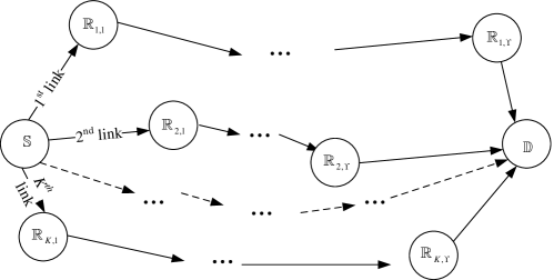
Refer to caption
Figure 1: Multihop Cooperative Communication System
Refer to caption
Figure 2: Banded Matrix Structure Approximation for 𝐃[𝐦~μ]𝐃delimited-[]subscript~𝐦𝜇\mathbf{D}[\mathbf{\tilde{m}}_{\mu}] and 𝐃[𝝃j]𝐃delimited-[]subscript𝝃𝑗\mathbf{D}[\boldsymbol{\xi}_{j}]
Refer to caption
Figure 3: Convergence of Channel Estimation for Dualhop OFDM System
Refer to caption
Figure 4: Convergence of Data Detection for Dualhop OFDM System
Refer to caption
Figure 5: Performance of Channel Estimation for Dualhop OFDM System
Refer to caption
Figure 6: Performance of Data Detection for Dualhop OFDM System
Refer to caption
Figure 7: Performance of Channel Estimation for Three-hop OFDM System
Refer to caption
Figure 8: Performance of Data Detection for Three-hop OFDM System