IGC-12/5-1


Holographic duals of Boundary CFTs111This work is supported in part by NSF grants PHY-08-55356 and PHY-07-57702.


Marco Chiodarolia, Eric Dโ€™Hokerb, Michael Gutperleb


a Institute for Gravitation and the Cosmos,
The Pennsylvania State University, University Park, PA 16802, USA

mchiodar@gravity.psu.edu


b Department of Physics and Astronomy
University of California, Los Angeles, CA 90095, USA
dhoker@physics.ucla.edu, gutperle@physics.ucla.edu;


Abstract

New families of regular half-BPS solutions to 6-dimensional Type 4b supergravity with $m$ tensor multiplets are constructed exactly. Their space-time consists of $AdS_{2}\times S^{2}$ warped over a Riemann surface with an arbitrary number of boundary components, and arbitrary genus. The solutions have an arbitrary number of asymptotic $AdS_{3}\times S^{3}$ regions. In addition to strictly single-valued solutions to the supergravity equations whose scalars live in the coset $SO(5,m)/SO(5)\times SO(m)$, we also construct stringy solutions whose scalar fields are single-valued up to transformations under the $U$-duality group $SO(5,m;{\bf Z})$, and live in the coset $SO(5,m;{\bf Z})\backslash SO(5,m)/SO(5)\times SO(m)$. We argue that these Type 4b solutions are holographically dual to general classes of interface and boundary CFTs arising at the juncture of the end-points of 1+1-dimensional bulk CFTs. We evaluate their corresponding holographic entanglement and boundary entropy, and discuss their brane interpretation. We conjecture that the solutions for which $\Sigma$ has handles and multiple boundaries correspond to the near-horizon limit of half-BPS webs of dyonic strings and three-branes.

1 Introduction and summary of results

The AdS/CFT correspondence relates string theory or M-theory on a space-time of the form $AdS_{d+1}\times M$ to a $d$-dimensional conformal field theory [1, 2, 3]. Generally, this CFT may be obtained directly from a system of branes in string theory or M-theory in the near-horizon limit where gravitational degrees of freedom decouple. The canonical example is provided by the duality between Type IIB string theory on $AdS_{5}\times S^{5}$ and 4-dimensional ${\cal N}=4$ super Yang-Mills theory obtained from the near-horizon limit of a stack of parallel D3-branes.

The AdS/CFT correspondence may be applied with equal success to space-times which are only asymptotically of the form $AdS_{d+1}\times M$, and their dual field theories which are conformal only in the UV limit. One example includes field theories with non-trivial renormalization group flow obtained by deforming a CFT by a relevant operator. In a second example, a CFT at finite temperature is dual to a gravity theory with a black hole or black brane horizon. Field theories with finite charge density, spontaneously broken symmetries, and confinement may all be realized by different types of gravitational solutions. In all of the cases given above, scale invariance is broken by the introduction of dimensionful couplings.

The field theories of interest to the present paper are characterized by the presence of an interface or a boundary. An interface CFT is obtained by gluing together several bulk CFTs at a common interface. A boundary CFT is obtained when a single bulk CFT ends on a boundary. When the interface or the boundary is flat, scale invariance may be preserved. The classification and construction of such interface and boundary CFTs constitutes a key problem in the study of CFTs which enjoys several physical applications (see e.g. [4] for a discussion of the two-dimensional case). While space-translations transverse to the interface or boundary are no longer symmetries, the Poincarรฉ transformations along the interface or boundary will be preserved. With a supersymmetric Yang-Mills theory in the bulk, various degrees of supersymmetry may be preserved by the interface or boundary, leading to theories with various superconformal symmetry invariances. A classification for the ${\cal N}=4$ case in 4 dimensions can be found in [5, 6].

On the gravity side, there are two complementary constructions of superconformal interface and boundary CFTs whose holographic duals are asymptotically $AdS_{5}\times S^{5}$:111Recently, an exact identification between these two constructions was obtained in [10, 11, 12].

  1. 1.

    Following [7, 8, 9], one considers intersecting brane configurations in flat space-time in which D3-branes can end on D5- and NS5-branes. In the near-horizon limit the world-volume theory on the D3-branes flows to a 4-dimensional interface or boundary CFT. Various half-BPS brane configurations then provide a natural classification of the boundary conditions which preserve a $OSp(4|4)$ superconformal symmetry [5, 6].

  2. 2.

    Fully back-reacted Type IIB supergravity solutions dual to an interface CFT can be constructed by using a Janus Ansatz [13], in which space-time is a fibration of $AdS_{4}\times S^{2}\times S^{2}$ over a two-dimensional Riemann surface $\Sigma$. In [14, 15]222For half-BPS solutions in M-theory see [16, 17, 18]. For related work by other authors see [19, 20, 21, 22, 23, 24, 25, 26, 27]. the corresponding half-BPS solutions with $OSp(4|4)$ symmetry were obtained exactly in terms of harmonic functions on $\Sigma$. A classification of all such half-BPS solutions in terms of superalgebras was given in [28].

1.1 Holographic duals to Interface and Boundary CFTs

A first goal of the present paper is to classify and construct the most general half-BPS solutions which are locally asymptotic to $AdS_{3}\times S^{3}$, and holographically dual to an interface or a boundary CFT in 2 space-time dimensions. A second goal is to derive physical quantities of the dual CFT, such as the holographic interface or boundary entropy. A third goal is to exhibit the precise map between these holographic solutions and intersecting brane configurations in flat space-time, in analogy with the results described above for the $AdS_{5}\times S^{5}$ case. In this paper, we shall achieve the first two goals, and make progress towards the third.

The problem of constructing half-BPS solutions dual to interface and boundary CFTs in two dimensions was attacked in [29, 30] directly in the language of Type IIB supergravity. There, space-time was of the form $AdS_{2}\times S^{2}\times K3$ warped over a Riemann surface $\Sigma$ with an arbitrary number of boundary components, but no handles. The solutions obtained are quarter-BPS from the point of view of 10-dimensional Type IIB supergravity, and thus invariant under 8 residual supersymmetries. In these solutions, however, only the volume form of the $K3$ manifold played a role, while the other homology generators of the $K3$, and their associated moduli, were turned off. Moreover, the supergravity fields, including the axion, were strictly single-valued, thereby excluding interesting quantum solutions.

The problem was also attacked in [31] in the language of the 6-dimensional Type 4b supergravity, a theory which arises as the dimensional reduction of Type IIB on $K3$. From the point of view of 6-dimensional Type 4b theory, the solutions are half-BPS and are again invariant under 8 residual supersymmetries. Type 4b supergravity has 5 self-dual and $21$ anti-self-dual 3-form fields, as well as 105 scalars living on the $SO(5,21)/SO(5)\times SO(21)$ coset [32]. This formulation has the distinct advantage of exhibiting the moduli of all $K3$ deformations on the same footing as the dilaton-axion scalars of Type IIB, and thus making the full U-duality group $SO(5,21;{\bf Z})$ manifest.

Type 4b supergravity lends itself well to identifying self-dual string solutions which carry the self-dual 3-form charge. Six-dimensional self-dual strings arise effectively from certain bound states of branes in 10-dimensional Type IIB string theory. The D1/D5 system with 4 worldvolume dimensions wrapped on $K3$ provides one example of such a self-dual string (the others can be obtained by the action of the U-duality group). In the near-horizon limit a self-dual string produces a supersymmetric $AdS_{3}\times S^{3}$ vacuum, invariant under the global superalgebra $PSU(1,1|2)\times PSU(1,1|2)$.

Much like $(p,q)$ strings of Type IIB in 10-dimensional flat Minkowski space-time [33, 34, 35], junctions where $N$ self-dual strings of Type 4b supergravity come together can be constructed in 6-dimensional Minkowski space-time. As discussed in [36] the supersymmetry algebra of 6-dimensional Type 4b supergravity contains a central charge $Z_{\mu}^{i}$ which is a Minkowski vector as well as a vector with respect of the $SO(5)$ R-symmetry. The central charge depends on the self-dual string charge and the spatial orientation of the self-dual string. Networks of self-dual strings are ${1\over 4}$-BPS in flat space-time provided they are planar and there is an alignment of the the spatial and $SO(5)$ directions of the central charge.

Apart from the self-dual strings, other supersymmetric branes exist in the 6-dimensional Minkowski vacuum. In particular, three-branes can be obtained from D3-branes, 5-branes wrapping 2-cycles of the $K3$, and D7-branes wrapping the whole $K3$. Since these branes are co-dimension two from the point of view of the 6 non-compact dimensions they induce non-trivial monodromy on the axionic scalars which enjoy a shift symmetry in the $SO(5,21)/SO(5)\times SO(21)$ coset. A novel feature of networks with three-branes is that self-dual strings can end on them. Charge conservation holds as the charge of the string is absorbed on the world-volume of the three-brane [37].

1.2 Novelties of the present solutions

In the present paper we shall complete the construction, which was initiated in [29, 30, 31], of the general half-BPS holographic solutions in 6-dimensional Type 4b supergravity, and thus in 10-dimensional Type IIB, which are dual to interface and boundary CFTs in two dimensions333Type 4b supergravity with $m=21$ can be obtained from the Kaluza-Klein compactification of Type IIB supergravity on K3. While it is unclear whether in general this truncation is consistent or not, solutions of the theory in six dimensions should uplift to 10-dimensional solutions in the limit in which the volume of the K3 is small.. The construction follows the Janus Ansatz with space-time geometry $AdS_{2}\times S^{2}$ warped over a Riemann surface $\Sigma$ with boundary. The novel results of the present solutions are as follows:

  1. 1.

    Building on the general local solutions of [31], the scalar fields in the present solutions take values in the largest sub-manifold of the scalar coset $SO(5,m)/SO(5)\times SO(m)$ allowed by the half-BPS condition, namely $SO(2,m)/SO(2)\times SO(m)$. By contrast, the solutions of [29, 30] were restricted to $SO(2,2)/SO(2)\times SO(2)$.

  2. 2.

    The present solutions allow for monodromy of the axionic scalars by elements of the U-duality group $SO(5,m;{\bf Z})$. This gives rise to stringy solutions in which the scalar fields live on a sub-manifold of the coset $SO(5,m;{\bf Z})\backslash SO(5,m)/SO(5)\times SO(m)$. By contrast, the scalar fields in the solutions of [29, 30, 31] were single-valued only.

  3. 3.

    The present solutions include surfaces $\Sigma$ with an arbitrary number of handles, producing an associated increase in the number of moduli. We conjecture that these solutions provide holographic duals to half-BPS networks of self-dual strings and three-branes in Type 4b. By contrast, the solutions of [29, 30, 31] excluded handles.

1.3 Overview of solutions dual to interface and boundary CFTs

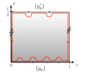
In the sequel of this introduction, we shall present an overview of the properties of all solutions, old and new, in more detail. The first ingredient in the solutions is a real harmonic function $H$ which is positive inside $\Sigma$ and vanishes on its boundary $\partial\Sigma$, except at a finite number $N$ of simple poles on $\partial\Sigma$. The region near each pole corresponds to a locally asymptotic $AdS_{3}\times S^{3}$ which is dual to a โ€œbulkโ€ CFT living on a half-space ${\bf R}^{+}\times{\bf R}$. The second ingredient is a set of $m$ meromorphic functions $L^{A}$, which are holomorphic inside $\Sigma$, are required to be real on $\partial\Sigma$, and have a finite number of simple poles on $\partial\Sigma$.

Refer to caption
Figure 1: (a) A junction of three self-dual strings in 6-dimensional flat space-time. (b) The corresponding Riemann surface $\Sigma$ for the dual holographic solution with $N=3$ poles. The blue cycles indicate three spheres on which the 3-form charges are supported.

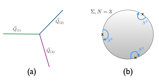
The simplest solutions are based on a Riemann surface $\Sigma$ with a single boundary component and no handles, namely the disk. They were constructed in [31], and will be briefly reviewed in Section 2. These solutions are holographic realizations of string junctions, where $N$ two-dimensional CFTs are glued together along a one-dimensional interface. The example of a three-string junction and its corresponding surface $\Sigma$ is depicted in Figure 1. These solutions can be obtained by taking a decoupling limit of ${1\over 4}$-BPS junction of $N$ self-dual strings in flat space-time. One argument for this identification is the exact match between the parameters of the supergravity solution and the physical quantities characterizing the string junction. Namely, the parameters of the solution can be identified with the 3-form charges on the asymptotic $S^{3}$, and the values of the scalars in the asymptotic region which are not fixed by the attractor mechanism.

The regular solutions constructed in [31] are dual to interface CFTs for $N=2$, and to the junction of $N$ CFTs for $N>2$. The dual to a boundary CFT should have $N=1$. Recently there has been a renewed interest in the holographic description of boundary CFTs [38, 39, 40, 41, 42, 43, 44]. No regular solutions with only one boundary were found in [31], but singular half-BPS solutions with $N=1$ were constructed in [45] as limits of regular interface solutions. The new type of singularities were referred to as the $AdS_{2}$-cap and $AdS_{2}$-funnel in [45].

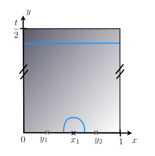
Perhaps the most important new result of the present paper is the construction of an infinite class of regular half-BPS solutions which are holographically dual to boundary CFTs. The simplest non-trivial case arises when $\Sigma$ is an annulus, with a single asymptotic $AdS_{3}\times S^{3}$ region. The configuration is illustrated in Figure 2, and will be solved for in detail in Section 4. The solution has non-trivial monodromy of the axionic scalars, and thus carries three-brane charge. Thus, we propose that this annulus solution is the holographic dual to a BCFT which is obtained as a decoupling limit of a self-dual string ending on a D3-brane.

Refer to caption
Figure 2: (a) A self-dual string ending on a three-brane in six dimensions. The charge of the string is absorbed on the three-brane. (b) Riemann surface $\Sigma$ for the dual BCFT solution with one pole. Near the pole a $S^{3}$ supports the charge, there is a second non-contractible $S^{1}\times S^{2}$ cycle.

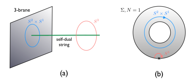
The annulus solution has two new features compared to the solutions on the disk. First, apart from the $S^{3}$-cycle associated with the asymptotic $AdS_{3}\times S^{3}$ region, there is a $S^{2}\times S^{1}$-cycle which appears because the annulus has a non-contractible $S^{1}$-cycle. This cycle can carry 3-form charge and hence charge conservation can be obeyed for a regular solution even when only a single asymptotic $AdS_{3}\times S^{3}$ region is present. Second, when transported along the non-contractible cycle of the annulus the scalars living in the $SO(5,21)/SO(5)\times SO(21)$ coset pick up a non-trivial Abelian monodromy. In supergravity, such a solution is not single-valued and therefore not regular. However, the stringy quantum moduli space of the theory is quotient of the $SO(5,21)/SO(5)\times SO(21)$ coset by the discrete U-duality group $SO(5,21;{\bf Z})$. If the monodromy identifies scalars by an Abelian subgroup of the U-duality group (i.e. a shift of axionic scalars) the resulting solution is regular in string theory. This monodromy indicates the presence of a three-brane in the 6-dimensional space-time444For a discussion of such branes in the probe approximation see e.g. [46, 47]..

In Section 5 we obtain the most general regular BPS solutions by considering Riemann surfaces $\Sigma$ which have $\nu$ boundary components, $g$ handles, and $N$ asymptotic $AdS_{3}\times S^{3}$ regions. The construction involves the double $\hat{\Sigma}$ of $\Sigma$, which is a compact Riemann surface of genus $\hat{g}=2g+\nu-1$. The harmonic and holomorphic functions which parametrize the solution are constructed using the prime form and holomorphic differentials, objects which are familiar from multi-loop string perturbation theory [48]. As for the annulus (which is a special case of the general solution with $g=0,\nu=2$) the solution displays non-trivial monodromy around non-contractible cycles. The solution is a proper string theory solution provided the scalar monodromy around each cycle is a U-duality transformation.

1.4 Conjecture on holographic duals to string networks

For any surface $\Sigma$, a solution whose harmonic function $H$ has $N$ poles can be interpreted as a holographic dual of a junction of $N$ CFTs each one living on a half-space. The charges and the values of the non-attracted scalars in each asymptotic region completely determine the CFTs which are glued together. The remaining parameters of the solution (which exist for all $\Sigma$ but the disk) should determine the gluing/boundary conditions at the junction. Hence the holographic solutions provide an infinite set of boundary and interface CFTs. It should be possible to calculate CFT junction correlation functions holographically, for any solution depending on its full set of free parameters, though technically this may be involved.

Refer to caption
Figure 3: (a) A configuration of three-branes and self-dual string networks. In the IR the system flows to a interface CFT. (b) A Riemann surface $\Sigma$ with $N=4$, $\nu=3$ and $g=1$.

The new feature of solutions with multiple boundary components are the non-trivial scalar monodromy and, relatedly, the presence of three-branes. For the annulus solution we provided some evidence that such a solution can be obtained from a decoupling/near-horizon limit of a self-dual string ending on a three-brane in 6-dimensional flat space-time.

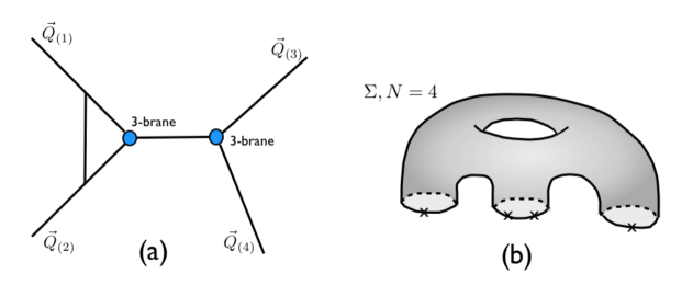
We conjecture that the most general solutions with arbitrary $g$ and $\nu$ can be obtained by taking a decoupling limit of a network of self-dual string and three-branes in flat space-time (see Figure 3a for an example of such a configuration). This situation should be analogous to the Gaiotto-Witten construction of 4-dimensional boundary and interface CFT discussed in the beginning of the Introduction. We have so far not been able to obtain a precise identification of the general supergravity solutions with a string and brane network. In particular the role of the handles is not well understood. We leave these question for future investigation.

The remainder of this paper is organized as follows. In Section 2, we briefly review Type 4b supergravity, the construction of half-BPS solutions by warping $AdS_{2}\times S^{2}$ over a Riemann surface $\Sigma$, and the solutions on the disk. In Section 3, we construct the general regular solutions for the case where $\Sigma$ is an annulus, and allow for solutions with monodromy in the U-duality group. In Section 4, the annulus solution for a single asymptotic $AdS_{3}\times S^{3}$ is worked out in detail, the associated boundary entropy is evaluated, and its degeneration is obtained. Finally, in Section 5, the most general regular half-BPS solution is constructed in terms of a Riemann surface $\Sigma$ with arbitrary number of boundary components, arbitrary number of asymptotic $AdS_{3}\times S^{3}$ regions, and arbitrary number of handles. We defer to the Appendix the lengthy calculation of the boundary entropy for the annulus.

2 Review of regular half-BPS solutions

In this section we shall briefly review the construction of half-BPS string-junction solutions in 6-dimensional Type $4b$ supergravity carried out in [31], which may be consulted for detailed derivations of the results.

2.1 Six dimensional Type $4b$ supergravity

The theory was constructed in [32]. We shall follow the notations and conventions of [31]. The supersymmetry of the Type $4b$ theory is generated by two symplectic-Majorana spinors. Type 4b contains a supergravity multiplet and $m$ tensor multiplets. Anomaly cancellation restricts the value of $m$ to the case of either $m=5$ or $m=21$, corresponding respectively to compactification of Type IIB on $T^{4}$ or $K3$. For definiteness we will principally work with the $K3$ compactification and choose $m=21$ in the sequel.555Throughout, the index $A=(I,R)$ will label the fundamental representation of $SO(5,m)$, while the indices $(i,r)$ will label the fundamental representation of $SO(5)\times SO(m)$. Their ranges are given by, $I,i=1,\ldots,5$ and $R,r=6,\ldots,m+5$ respectively. The supergravity multiplet contains the metric and the Rarita-Schwinger field as well as five rank-two anti-symmetric tensors $B^{I}$. Each tensor multiplet contains an anti-symmetric rank-two tensor $B^{R}$, and a quartet of Weyl fermions whose chirality is opposite to that of the gravitini. Finally, the scalar fields live in the real $SO(5,m)/(SO(5)\times SO(m))$ coset space and are parametrized by a real frame field $V^{i,r}_{\;\;A}$. They may be represented by composite 1-form fields $P^{ir}$, $Q^{ij}$ and Srโ€‹ssuperscript๐‘†๐‘Ÿ๐‘ S^{rs} which are the block components of $V^{-1}dV$. The 2-form potentials $B^{A}_{\mu\nu}$ give rise to field strength 3-forms, $G^{A}=dB^{A}$. The associated $SO(5,m)$-covariant field strength 3-forms $H^{i}$ and $H^{r}$, which are respectively self-dual and anti-self-dual, obey,

$\displaystyle H^{i}=V^{i}{}_{A}\,G^{A}$ $\displaystyle*H^{i}=+H^{i}$
$\displaystyle H^{r}=V^{r}{}_{A}\,G^{A}$ $\displaystyle*H^{r}=-H^{r}$ (2.1)

The fields $H^{i}$ and $H^{r}$ obey Bianchi identities which follow from $dG^{A}=0$,

$\displaystyle dH^{i}-Q^{ij}\wedge H^{j}-\sqrt{2}P^{ir}\wedge H^{r}$ $\displaystyle=$ $\displaystyle 0$
dโ€‹Hrโˆ’Srโ€‹sโˆงHsโˆ’2โ€‹Piโ€‹rโˆงHi๐‘‘superscript๐ป๐‘Ÿsuperscript๐‘†๐‘Ÿ๐‘ superscript๐ป๐‘ 2superscript๐‘ƒ๐‘–๐‘Ÿsuperscript๐ป๐‘–\displaystyle dH^{r}-S^{rs}\wedge H^{s}-\sqrt{2}P^{ir}\wedge H^{i} $\displaystyle=$ $\displaystyle 0$ (2.2)

For the field strengths $H^{i}$ and $H^{r}$, the Bianchi identities and field equations are equivalent to one another in view of their duality properties. The Einstein equations are given by,

$$R_{\mu\nu}-H^{i}_{\mu\rho\sigma}H^{i\;\rho\sigma}_{\nu}-H^{r}_{\mu\rho\sigma}H^{r\;\rho\sigma}_{\nu}-2P_{\mu}^{ir}P_{\nu}^{ir}=0$$ (2.3)

The field equation for the scalars is given by,

โˆ‡ฮผPฮผiโ€‹rโˆ’(Qฮผ)iโ€‹jโ€‹Pฮผjโ€‹rโˆ’(Sฮผ)rโ€‹sโ€‹Pฮผiโ€‹sโˆ’23โ€‹Hiโ€‹ฮผโ€‹ฮฝโ€‹ฯโ€‹Hฮผโ€‹ฮฝโ€‹ฯr=0superscriptโˆ‡๐œ‡superscriptsubscript๐‘ƒ๐œ‡๐‘–๐‘Ÿsuperscriptsuperscript๐‘„๐œ‡๐‘–๐‘—superscriptsubscript๐‘ƒ๐œ‡๐‘—๐‘Ÿsuperscriptsuperscript๐‘†๐œ‡๐‘Ÿ๐‘ superscriptsubscript๐‘ƒ๐œ‡๐‘–๐‘ 23superscript๐ป๐‘–๐œ‡๐œˆ๐œŒsubscriptsuperscript๐ป๐‘Ÿ๐œ‡๐œˆ๐œŒ0\nabla^{\mu}P_{\mu}^{ir}-(Q^{\mu})^{ij}P_{\mu}^{jr}-(S^{\mu})^{rs}P_{\mu}^{is}-{\sqrt{2}\over 3}H^{i\;\mu\nu\rho}H^{r}_{\mu\nu\rho}=0 (2.4)

The fermionic fields $\psi_{\mu}^{\alpha}$ and $\chi^{r\alpha}$ of the Type 4b supergravity, as well as the local supersymmetry spinor parameter $\varepsilon^{\alpha}$, have definite chiralities, and obey the symplectic Majorana conditions. The BPS equations are given by,666The Dirac matrices $\gamma^{\mu}$ with respect to coordinate indices are related to the Dirac matrices $\gamma^{M}$ with respect to frame indices by $\gamma^{M}=e^{M}{}_{\mu}\gamma^{\mu}$.

$\displaystyle 0$ $\displaystyle=$ $\displaystyle\partial_{\mu}\varepsilon^{\alpha}+{1\over 4}\omega_{\mu}^{MN}\gamma_{MN}\varepsilon^{\alpha}-{1\over 4}Q_{\mu}^{ij}(\Gamma^{ij})^{\alpha}{}_{\beta}\,\varepsilon^{\beta}-{1\over 4}H^{i}_{\mu\nu\rho}\gamma^{\nu\rho}\;(\Gamma^{i})^{\alpha}_{\;\;\beta}\varepsilon^{\beta}$
$\displaystyle 0$ $\displaystyle=$ $\displaystyle{1\over\sqrt{2}}\gamma^{\mu}P_{\mu}^{ir}(\Gamma^{i})^{\alpha}_{\;\;\beta}\varepsilon^{\beta}+{1\over 12}\gamma^{\mu\nu\rho}H^{r}_{\mu\nu\rho}\varepsilon^{\alpha}$ (2.5)

The theory has a 6-dimensional Minkowski space-time vacuum where all anti-symmetric tensor fields are set to zero, and which is invariant under 16 Poincarรฉ supersymmetries. Self-dual BPS string solutions can be constructed which preserve 8 of the 16 Poincarรฉ supersymmetries. The $AdS_{3}\times S^{3}$ vacuum with 16 supersymmetries and $PSU(1,1|2)\times PSU(1,1|2)$ symmetry superalgebra emerges in the near-horizon limit.

2.2 Regular half-BPS solutions

The geometry of a local half-BPS string-junction solution in six dimensions consists of an $AdS_{2}\times S^{2}$ space warped over a two-dimensional Riemann surface $\Sigma$ with boundary [29, 31]. The metric and anti-symmetric tensor fields of the solution are,

dโ€‹s2๐‘‘superscript๐‘ 2\displaystyle ds^{2} $\displaystyle=$ f12โ€‹dโ€‹sAโ€‹dโ€‹S22+f22โ€‹dโ€‹sS22+dโ€‹sฮฃ2superscriptsubscript๐‘“12๐‘‘subscriptsuperscript๐‘ 2๐ด๐‘‘subscript๐‘†2superscriptsubscript๐‘“22๐‘‘subscriptsuperscript๐‘ 2superscript๐‘†2๐‘‘subscriptsuperscript๐‘ 2ฮฃ\displaystyle f_{1}^{2}ds^{2}_{AdS_{2}}+f_{2}^{2}ds^{2}_{S^{2}}+ds^{2}_{\Sigma}
$\displaystyle B^{A}$ $\displaystyle=$ $\displaystyle\Psi^{A}\,\omega_{AdS_{2}}+\Phi^{A}\,\omega_{S^{2}}$ (2.6)

Here, dโ€‹sAโ€‹dโ€‹S22๐‘‘subscriptsuperscript๐‘ 2๐ด๐‘‘subscript๐‘†2ds^{2}_{AdS_{2}} and dโ€‹sS22๐‘‘subscriptsuperscript๐‘ 2superscript๐‘†2ds^{2}_{S^{2}} are the invariant metrics respectively on the spaces $AdS_{2}$ and $S^{2}$ of unit radius, while $\omega_{AdS_{2}}$ and $\omega_{S^{2}}$ are the corresponding volume forms. In local complex coordinates $(w,\bar{w})$ on $\Sigma$, the metric dโ€‹sฮฃ2=4โ€‹ฯ2โ€‹|dโ€‹w|2๐‘‘superscriptsubscript๐‘ ฮฃ24superscript๐œŒ2superscript๐‘‘๐‘ค2ds_{\Sigma}^{2}=4\rho^{2}|dw|^{2} is parametrized by a real function $\rho$.

The general local solution was constructed in [31] and is specified completely in terms of a real positive harmonic function $H$ and $m+2$ meromorphic functions $\lambda^{A}$ on $\Sigma$. Solving the BPS equations, Bianchi identities, and field equations, subject to the reality of the fields, imposes the restriction $\lambda^{3}=\lambda^{4}=\lambda^{5}=0$, (up to $SO(5,m)$ transformations), as well as,777Throughout, we shall use the $SO(5,m)$-invariant metric $\eta={\rm diag}(I_{5},-I_{m})$ to raise and lower indices $K^{A}=\eta^{AB}K_{B}$ for vectors $K\in{\bf C}^{5,m}$, and to form their inner invariant product $K\cdot L=\eta_{AB}K^{A}L^{B}$.

$\displaystyle\lambda\cdot\lambda$ $\displaystyle=$ $\displaystyle 2$
$\displaystyle\bar{\lambda}\cdot\lambda$ $\displaystyle\geq$ $\displaystyle 2$ (2.7)

with strict inequality of the second condition in the interior of $\Sigma$. The solution of [31] provides explicit formulas for the metric factors,

$\displaystyle f_{1}^{4}=H^{2}~{}{\bar{\lambda}\cdot\lambda+2\over\bar{\lambda}\cdot\lambda-2}$ $\displaystyle\rho^{4}={|\partial_{w}H|^{4}\over 16H^{2}}(\bar{\lambda}\cdot\lambda+2)(\bar{\lambda}\cdot\lambda-2)$
$\displaystyle f_{2}^{4}=H^{2}~{}{\bar{\lambda}\cdot\lambda-2\over\bar{\lambda}\cdot\lambda+2}$ (2.8)

On the solutions, the scalar field $V$ takes values in an $SO(2,m)/(SO(2)\times SO(m))$ sub-manifold of the real coset space $SO(5,m)/(SO(5)\times SO(m))$, so that $V$ takes the form,

$\displaystyle V=\left(\begin{array}[]{ccc}V^{i}{}_{I}&0&V^{i}{}_{R}\cr 0&I_{3}&0\cr V^{r}{}_{I}&0&V^{r}{}_{R}\cr\end{array}\right)$ (2.12)

where $i,I=1,2$, and $r,R=6,\ldots,m+5$. The block $I_{3}$ represents the identity in the indices $i,I=3,4,5$. The combinations $V^{\pm}_{I,R}=V^{1}_{I,R}\pm iV^{2}_{I,R}$ may be expressed in terms of the functions $H$ and $\lambda^{A}$, up to an overall phase which depends on the choice of gauge, by the relation,

$\displaystyle V^{+}{}_{A}=X(\bar{\lambda}_{A}-|X|^{2}\lambda_{A})/(1-|X|^{4})$ (2.13)

and its complex conjugate $V^{-}_{A}$, where $A=1,2,6,7,\ldots,m+5$, and $|X|$ is given by $|X|^{2}+|X|^{-2}=\lambda\cdot\bar{\lambda}$. The remaining entries of $V$ contain no further degrees of freedom and may be derived from the defining property for the $SO(5,m)$ frame, $V^{-1}=\eta V^{t}\eta$. On the solutions, the anti-symmetric tensor fields $B^{A}$ are subject to the restriction $B^{3}=B^{4}=B^{5}=0$, which parallels the restriction of the scalars. The solutions for the remaining components of the real-valued flux potential functions $\Phi^{A}$ and $\Psi^{A}$ are as follows,

$\displaystyle\Phi^{A}=-\sqrt{2}\,{H\,{\rm Re}(\lambda^{A})\over\bar{\lambda}\cdot\lambda+2}+\tilde{\Phi}^{A}$ $\displaystyle\tilde{\Phi}^{A}={1\over 2\sqrt{2}}\int\partial_{w}H\,\lambda^{A}+{\rm c.c.}$
$\displaystyle\Psi^{A}=-\sqrt{2}\,{H\,{\rm Im}(\lambda^{A})\over\bar{\lambda}\cdot\lambda-2}+\tilde{\Psi}^{A}$ $\displaystyle\tilde{\Psi}^{A}={i\over 2\sqrt{2}}\int\partial_{w}H\,\lambda^{A}+{\rm c.c.}$ (2.14)

where again $A=1,2,6,7,\ldots,m+5$.

The metric and other fields will be regular throughout $\Sigma$, provided the harmonic function $H$ and the meromorphic functions $\lambda^{A}$ satisfy the following regularity requirements,

1. In the interior of $\Sigma$ we have $H>0$ and $\bar{\lambda}\cdot\lambda>2$;

2. On the boundary $\partial\Sigma$ of $\Sigma$ we have $H=0$ and ${\rm Im}(\lambda^{A})=0$, except at isolated points;

3. The 1-forms $\lambda^{A}\partial_{w}H$ are holomorphic and nowhere vanishing in the interior of $\Sigma$, forcing the poles of $\lambda^{A}$ to coincide with the zeros of $\partial_{w}H$;

4. The functions $\lambda^{A}$ are holomorphic near $\partial\Sigma$, thereby allowing for poles in $\lambda^{A}\partial_{w}H$ on $\partial\Sigma$ only at those points where $\partial_{w}H$ has a pole.

In [45], a mild relaxation of some of these regularity conditions was shown to lead to generalized solutions, which are still physically acceptable. They include the $AdS_{2}$-cap and the $AdS_{2}$-funnel, which may be interpreted as fully back-reacted brane solutions and give simple, though singular, examples of holographic boundary CFTs.

2.3 Light-cone variables

A general explicit solution of the constraints (2.2) and the regularity requirements $1-4$ of Section 2.2 may be obtained following [31] by parametrizing the functions $\lambda^{A}$ in terms of light-cone variables $L^{A}$, defined by,

$\displaystyle\lambda^{A}={\sqrt{2}\,L^{A}\over L^{6}}\hskip 28.90755pt$ $\displaystyle\lambda^{+}={\sqrt{2}\over L^{6}}\left(-L^{1}L^{1}+L^{R}L^{S}\delta_{RS}\right)$
$\displaystyle\lambda^{\pm}={1\over\sqrt{2}}(\lambda^{2}\pm\lambda^{6})$ $\displaystyle\lambda^{-}={1\over\sqrt{2}L^{6}}$ (2.15)

where the indices run over $A=1,7,8,\ldots,m+5$, and $R,S=6,7,8,\ldots,m+5$. This parametrization explicitly solves the first constraint of (2.2). Multiplication of $L^{6}$ and $L^{A}$ by a common constant $\ell$ leaves the $\lambda^{A}$ unchanged, but transforms $\lambda^{\pm}$ by an $SO(5,m)$ boost, $\lambda^{\pm}\to\ell^{\pm 1}\lambda^{\pm}$. Since the $\lambda^{A}$ are meromorphic, the functions $L^{A}$ must also be meromorphic. Moreover, the harmonic functions $h^{A}={\rm Im}(L^{A})$ associated with $L^{A}$ must obey Dirichlet vanishing conditions,

$\displaystyle h^{A}=0\quad\hbox{on}\quad\partial\Sigma$ (2.16)

With the help of the following relation,

$\displaystyle\bar{\lambda}\cdot\lambda-2={4\over|L^{6}|^{2}}\left((h^{1})^{2}-\sum_{R=6}^{m+5}(h^{R})^{2}\right)$ (2.17)

the second constraint of (2.2) may be translated into the following inequality, which is strict in the interior of $\Sigma$,

$\displaystyle(h^{1})^{2}>\sum_{R=6}^{m+5}(h^{R})^{2}$ (2.18)

The construction of [31] specializes to the case where $\Sigma$ has only one boundary component, i.e. $\Sigma$ is a the disk. The light-cone variables introduced here in (2.3) and the conditions for regularity of (2.16) and (2.18) hold, however, for general Riemann surfaces $\Sigma$ with arbitrary numbers of boundary components.

2.4 Regular solutions for the disk or upper-half-plane

The simplest Riemann surface $\Sigma$ for which our half-BPS solutions can be constructed has one boundary and can be represented by a disk of unit radius. In the following we conformally map the disk to the upper half-plane where the boundary is given by the real line. The harmonic function $H$ is restricted by the regularity conditions to be of the form,

$\displaystyle H(w,\bar{w})=\sum_{n=1}^{N}\left({i\,c_{n}\over w-x_{n}}-{i\,c_{n}\over\bar{w}-x_{n}}\right)\hskip 72.26999ptc_{n}>0$ (2.19)

The meromorphic light-cone functions $L^{A}$ may be parametrized by a finite number of simple (auxiliary) poles and take the form,

$\displaystyle L^{A}(w)=\ell^{A}_{\infty}+\sum^{P}_{p=1}{\ell^{A}_{p}\over w-y_{p}}$ (2.20)

The positions of the poles $y_{p}$, their residues $\ell^{A}_{p}$, and the values $\ell^{A}_{\infty}$ must all be real, and the index runs over $A=1,6,7,\ldots,m+5$. Regularity of the solutions requires that all the zeros of $L^{6}$ and $\partial_{w}H$ be common, and that $L^{6}$ be regular at the poles of $\partial_{w}H$. Therefore, $L^{6}$ may be expressed as follows,

$\displaystyle L^{6}(w)=i\tilde{\ell}^{6}_{\infty}{\prod_{n}^{N}(w-x_{n})^{2}\over\prod_{p}^{P}(w-y_{p})}\partial_{w}H(w)$ (2.21)

Matching between the expressions for $L^{6}$ given in (2.20) and (2.21) requires the number of auxiliary poles $P$ to be related to the number of physical poles $N$, by the relation $P=2N-2$, and the constants at $\infty$ to obey the relation $\ell^{6}_{\infty}=\tilde{\ell}^{6}_{\infty}\sum_{n=1}^{N}c_{n}$. Finally, regularity of the $\lambda^{A}$ at the auxiliary poles, and constancy of the sign of $h_{1}<0$, require the relation,

$$\ell^{1}_{p}=\left(\sum_{R=6}^{m+5}\ell_{p}^{R}\ell_{p}^{R}\right)^{1\over 2}$$ (2.22)

As a result of the Schwarz inequality, condition (2.18) is then automatically satisfied.
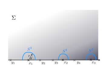
Refer to caption
Figure 4: Holographic string-junction solution with $N=3$ asymptotic $AdS_{3}\times S^{3}$ regions localized at the poles $x_{n}$, with $n=1,2,3$ and $P=4$ auxiliary poles at $y_{p}$, with $p=1,2,3,4$. Each homology $S^{3}$ is realized as an $S^{2}$ fibered over a line interval $C(x_{n})$ represented here by a half-circle in blue.

Near the location $x_{n}$ of a pole of $H$ the metric takes the following form,

dโ€‹s2โˆผRn2โ€‹(dโ€‹r2r2+rn2r2โ€‹dโ€‹sAโ€‹dโ€‹S22+dโ€‹ฮธ2+sin2โกฮธโ€‹dโ€‹sS22)+๐’ชโ€‹(r2)similar-to๐‘‘superscript๐‘ 2superscriptsubscript๐‘…๐‘›2๐‘‘superscript๐‘Ÿ2superscript๐‘Ÿ2superscriptsubscript๐‘Ÿ๐‘›2superscript๐‘Ÿ2๐‘‘superscriptsubscript๐‘ ๐ด๐‘‘subscript๐‘†22๐‘‘superscript๐œƒ2superscript2๐œƒ๐‘‘superscriptsubscript๐‘ superscript๐‘†22๐’ชsuperscript๐‘Ÿ2ds^{2}\sim R_{n}^{2}\left({dr^{2}\over r^{2}}+{r_{n}^{2}\over r^{2}}ds_{AdS_{2}}^{2}+d\theta^{2}+\sin^{2}\theta\,ds_{S^{2}}^{2}\right)+{\cal O}(r^{2})

where $w=x_{n}+re^{i\theta}$, as depicted in Figure 4. As $r\to 0$ the geometry approaches that of an asymptotic $AdS_{3}\times S^{3}$ region. The radius parameters $R_{n}$ and $r_{n}$ at a pole $x_{n}$ are determined by the asymptotic AST charge $Q_{n}^{A}$ as follows,888These results correspond to formula (7.14) of [31], with $\mu^{A}_{n}$ re-expressed in terms of $Q_{n}^{A}$ using (7.15).

$\displaystyle R_{n}^{4}={Q_{n}\cdot Q_{n}\over 4\pi^{4}}\hskip 72.26999ptr_{n}^{2}={16\pi^{4}c_{n}^{2}\over Q_{n}\cdot Q_{n}}$ (2.23)

The charges $Q^{A}_{n}$ may be expressed directly in terms of the parameters of the solution by,

$$Q^{A}_{n}\equiv\oint_{(S^{3})_{n}}dB^{A}=\sqrt{2}\pi\int_{C(x_{n})}\!\!dw\,\partial_{w}H\,\lambda^{A}+{\rm c.c.}=2\sqrt{2}\pi^{2}c_{n}\partial\lambda^{A}(x_{n})$$ (2.24)

The asymptotic charge is supported by an $S^{3}$ which is realized here by fibering an $S^{2}$ over small semi-circle $C(x_{n})$ surrounding the pole $x_{n}$, as depicted in Figure 4.

As explained in detail in [29] the holographic interpretation of these solutions as interface theories proceeds as follows: each region near a pole of $H$ produces a holographic boundary component on which a CFT defined on a half-space lives. The boundaries of these half-spaces are glued together along a one-dimensional interface which is given by the boundary of the $AdS_{2}$ factor.

The counting of moduli of the space of solutions on the disk with $N$ poles is presented in Table 1,

parameters number
$x_{n}$ $N$
$c_{n}$ $N$
$y_{p}$ $2N-2$
$l_{p}^{R}$ $(m-1)(2N-2)$
$l^{A}_{\infty}$ $m+1$
$SL(2,R)$ $-3$
Table 1: Moduli counting for the half-plane yielding a total of $2(m+1)N-m-2$.

where the total number of moduli of the solution is found to be $2(m+1)N-m-2$. This counting agrees with the corresponding counting of the number of physical parameters. We have $(m+2)(N-1)$ charges, where the number of independent asymptotic charges (2.24) is reduced from $N$ to $N-1$ because of charge conservation. In addition there are the $m$ scalars whose values are not fixed by the attractor mechanism in each asymptotic region giving $mN$ parameters. The total number of physical parameters agrees with the number of moduli given in Table 1.

3 Half-BPS solutions on the annulus

The aim of the present paper is to construct string-junction solutions for Riemann surfaces $\Sigma$ of general topology and arbitrary moduli. In this section, we shall take a first step in this direction, and consider the simplest case of a surface $\Sigma$ with two disconnected boundary components, namely an annulus. We shall describe the construction of the annulus solutions in detail here since it provides a very explicit example of the methods that will be used to construct the solutions for general Riemann surface $\Sigma$ in Section 5.

The annulus has a single imaginary modular parameter $\tau=it$ where $t$ is real and may be taken to be positive. We introduce complex coordinates $w,\bar{w}$, subject to the identification $w\sim w+1$, so that $\Sigma$ may be represented by a rectangular domain in the complex plane,

$\displaystyle\Sigma=\left\{w\in\mathbf{C},~{}~{}0\leq{\rm Re}(w)<1,~{}~{}0\leq{\rm Im}(w)\leq{t\over 2}\right\}$ (3.1)

The two disconnected boundary components of $\partial\Sigma$ are specified respectively by ${\rm Im}(w)=0$ and ${\rm Im}(w)=t/2$. As is customary, we make use of the compact double Riemann surface $\hat{\Sigma}$, which is a torus, and is defined by,

$\displaystyle\hat{\Sigma}=\left\{w\in\mathbf{C},~{}~{}0\leq{\rm Re}(w)<1,~{}~{}-{t\over 2}<{\rm Im}(w)\leq{t\over 2}\right\}$ (3.2)

together with the identifications $w\sim w+1$ and $w\sim w+it$. Under the anti-conformal involution of complex conjugation $\phi(w)=\bar{w}$, we may identify $\Sigma$ as the coset $\Sigma=\hat{\Sigma}/\phi$.

3.1 Solving for $H$ and $h^{A}$

The constructions of the real harmonic functions $H$ and $L^{A}={\rm Im}(L^{A})$, used in the light-cone parametrization of the local solution, will proceed in parallel to one another, and may be systematically derived in all generality.

One key requirement is that we have $H=h^{A}=0$ on $\partial\Sigma$, following (2.16). A second key requirement is that $H$ must be positive inside $\Sigma$, so that it cannot have poles in the interior of $\Sigma$. Thus, the poles of $H$ must be distributed on the two boundary components of $\Sigma$, and will be denoted respectively by $x_{n}$ and $\tau/2+x^{\prime}_{n^{\prime}}$ where the parameters $x_{n}$ and $x^{\prime}_{n^{\prime}}$ are real, and the corresponding indices run over $n=1\ldots,N$ and ${n^{\prime}}=1,\ldots,N^{\prime}$.

To specify the meromorphic functions $L^{A}$, it will be convenient to first construct their associated real harmonic functions $h^{A}={\rm Im}(L^{A})$. In view of the strict inequality (2.18) in the interior of $\Sigma$, we see that $h^{1}$ cannot vanish inside $\Sigma$, and every pole of $h^{R}$ must be a pole of $h^{1}$. As a result, all the poles of $h^{1}$, and thus all the poles of $h^{A}$, must be on the boundary of $\Sigma$. These auxiliary poles will be denoted respectively by $y_{p}$ and $\tau/2+y^{\prime}_{p^{\prime}}$, where the parameters $y_{p}$ and $y^{\prime}_{p^{\prime}}$ are real, and the indices run over $p=1,\ldots,P$, and ${p^{\prime}}=1,\ldots,P^{\prime}$.

In view of their single-valuedness on the double surface $\hat{\Sigma}$, the harmonic functions $H$ and $h^{A}$ must be doubly periodic, namely with periods $1$ and $\tau=it$. They are uniquely, but formally, obtained by summing over the contributions of all respective poles,

$\displaystyle H$ $\displaystyle\sim$ โˆ’2โ€‹Imโ€‹โˆ‘(r,s)โˆˆ๐™2(โˆ‘n=1Ncnwโˆ’xnโˆ’rโˆ’sโ€‹ฯ„+โˆ‘nโ€ฒ=1Nโ€ฒcnโ€ฒโ€ฒwโˆ’xnโ€ฒโ€ฒโˆ’rโˆ’sโ€‹ฯ„)2Imsubscript๐‘Ÿ๐‘ superscript๐™2superscriptsubscript๐‘›1๐‘subscript๐‘๐‘›๐‘คsubscript๐‘ฅ๐‘›๐‘Ÿ๐‘ ๐œsuperscriptsubscriptsuperscript๐‘›โ€ฒ1superscript๐‘โ€ฒsubscriptsuperscript๐‘โ€ฒsuperscript๐‘›โ€ฒ๐‘คsubscriptsuperscript๐‘ฅโ€ฒsuperscript๐‘›โ€ฒ๐‘Ÿ๐‘ ๐œ\displaystyle-2\,{\rm Im}\sum_{(r,s)\in{\bf Z}^{2}}\left(\sum_{n=1}^{N}{c_{n}\over w-x_{n}-r-s\tau}+\sum_{{n^{\prime}}=1}^{N^{\prime}}{c^{\prime}_{n^{\prime}}\over w-x^{\prime}_{n^{\prime}}-r-s\tau}\right)
$\displaystyle h^{A}$ $\displaystyle\sim$ Imโ€‹โˆ‘(r,s)โˆˆ๐™2(โˆ‘p=1Pโ„“pAwโˆ’ypโˆ’rโˆ’sโ€‹ฯ„+โˆ‘pโ€ฒ=1Pโ€ฒโ„“pโ€ฒโ€ฒโฃAwโˆ’ypโ€ฒโ€ฒโˆ’rโˆ’sโ€‹ฯ„)Imsubscript๐‘Ÿ๐‘ superscript๐™2superscriptsubscript๐‘1๐‘ƒsubscriptsuperscriptโ„“๐ด๐‘๐‘คsubscript๐‘ฆ๐‘๐‘Ÿ๐‘ ๐œsuperscriptsubscriptsuperscript๐‘โ€ฒ1superscript๐‘ƒโ€ฒsubscriptsuperscriptโ„“โ€ฒ๐ดsuperscript๐‘โ€ฒ๐‘คsubscriptsuperscript๐‘ฆโ€ฒsuperscript๐‘โ€ฒ๐‘Ÿ๐‘ ๐œ\displaystyle{\rm Im}\sum_{(r,s)\in{\bf Z}^{2}}\left(\sum_{p=1}^{P}{\ell^{A}_{p}\over w-y_{p}-r-s\tau}+\sum_{{p^{\prime}}=1}^{P^{\prime}}{\ell^{\prime A}_{p^{\prime}}\over w-y^{\prime}_{p^{\prime}}-r-s\tau}\right) (3.3)

The sums over integers (r,s)๐‘Ÿ๐‘ (r,s) are logarithmically divergent and may be regularized by adding functions linear and constant in $w$. The corresponding regularized sums are readily recognized to be related to the Weierstrass $\zeta(w)$ function. For our purposes, it will be more convenient to work with the following function,

$\displaystyle\zeta_{0}(w)\equiv{\partial_{w}\vartheta_{1}(w)\over\vartheta_{1}(w)}+{2\pi iw\over\tau}$ (3.4)

where $\vartheta_{1}(w)=\vartheta_{1}(w|\tau)$ is the Jacobi $\vartheta$-function, satisfying the periodicity relations,

$\displaystyle\vartheta_{1}(w+1)$ $\displaystyle=$ $\displaystyle-\vartheta_{1}(w)$
$\displaystyle\vartheta_{1}(w+\tau)$ $\displaystyle=$ $\displaystyle-e^{-i\pi(2w+\tau)}\vartheta_{1}(w)$ (3.5)

The functions $\zeta(w)$ and $\zeta_{0}(w)$ differ from one another by a term linear in $w$, which has been chosen so that $\zeta_{0}(w)$ is periodic in $w$ with imaginary period $\tau$. The remaining non-trivial monodromy of $\zeta_{0}(w)$ is then given by,

$\displaystyle\zeta_{0}(w+1)=\zeta_{0}(w)+{2\pi i\over\tau}$ (3.6)

The harmonic function $h_{0}(w)\equiv-{\rm Im}\,\zeta_{0}(w)$ enjoys the following properties,

  1. 1.

    $h_{0}=-{\rm Im}\,\zeta_{0}$ vanishes on $\partial\Sigma$, namely when $w\in{\bf R}$ and when $w-\tau/2\in{\bf R}$;

  2. 2.

    $h_{0}=-{\rm Im}\,\zeta_{0}>0$ in the interior of $\Sigma$.

Using the above properties, we are now in a position to write precise formulas for the harmonic functions $H$ and $h^{A}$ (instead of the formal expressions of (3.1)), and we find,

$\displaystyle H$ $\displaystyle=$ $\displaystyle-2\,{\rm Im}\sum_{n=1}^{N}c_{n}\,\zeta_{0}(w-x_{n})-2\,{\rm Im}\sum_{{n^{\prime}}=1}^{N^{\prime}}c^{\prime}_{n^{\prime}}\,\zeta_{0}(w^{\prime}+x^{\prime}_{n^{\prime}})$
$\displaystyle h^{A}$ $\displaystyle=$ $\displaystyle{\rm Im}\sum_{p=1}^{P}\ell^{A}_{p}\,\zeta_{0}(w-y_{p})+{\rm Im}\sum_{{p^{\prime}}=1}^{P^{\prime}}\ell^{\prime A}_{p^{\prime}}\,\zeta_{0}(w^{\prime}+y^{\prime}_{p^{\prime}})$ (3.7)

Throughout, we shall use the shorthand notation,

$\displaystyle w^{\prime}={\tau\over 2}-w$ (3.8)

The vanishing of $H$ and $h^{A}$ on both boundary components of $\Sigma$ requires the residues $c_{n},\ell^{A}_{p},c^{\prime}_{n^{\prime}},\ell^{\prime A}_{p^{\prime}}$ to be real. Positivity of $H$ throughout the interior of $\Sigma$ in turn requires,

$\displaystyle c_{n}>0$ $\displaystyle n=1,\dots,N$
$\displaystyle c^{\prime}_{n^{\prime}}>0$ $\displaystyle{n^{\prime}}=1,\dots,N^{\prime}$ (3.9)

3.2 Parametrizing $L^{A}$

The meromorphic functions $L^{A}$, for $A=1,6,7,\ldots,m+5$, may be inferred from the form of the harmonic functions $h^{A}$, and we find,

$\displaystyle L^{A}=L_{0}^{A}+\sum_{p=1}^{P}\ell^{A}_{p}\,\zeta_{0}(w-y_{p})+\sum_{{p^{\prime}}=1}^{P^{\prime}}\ell^{\prime A}_{p^{\prime}}\,\zeta_{0}(w^{\prime}+y^{\prime}_{p^{\prime}})$ (3.10)

where $L_{0}^{A}$ are real constants whose values are undetermined by $h^{A}$. Whereas the harmonic functions $h^{A}$ have been constructed to be single-valued on the annulus, the corresponding meromorphic functions $L^{A}$ may have additive monodromy,

$\displaystyle L^{A}(w+1)=L^{A}(w)+K^{A}\hskip 72.26999ptK^{A}={2\pi i\over\tau}\left(\sum_{p=1}^{P}\ell^{A}_{p}-\sum_{{p^{\prime}}=1}^{P^{\prime}}\ell^{\prime A}_{p^{\prime}}\right)$ (3.11)

The light-cone construction requires $L^{6}$ to be single-valued on the boundary $\partial\Sigma$, so that we must impose the following relation,

$\displaystyle 0=K^{6}=\sum_{p=1}^{P}\ell^{6}_{p}-\sum_{{p^{\prime}}=1}^{P^{\prime}}\ell^{\prime 6}_{p^{\prime}}$ (3.12)

As a result, $L^{6}$ is a doubly periodic function with periods 1 and $\tau$. The absence of second order auxiliary poles in $\lambda^{2}$, $\lambda^{6}$ at both boundary components requires,

$\displaystyle\ell^{1}_{p}=\left(\sum_{R=6}^{m+5}(\ell_{p}^{R})^{2}\right)^{1\over 2}\hskip 72.26999pt\ell^{\prime 1}_{p^{\prime}}=\left(\sum_{R=6}^{m+5}(\ell_{p^{\prime}}^{\prime R})^{2}\right)^{1\over 2}$ (3.13)

both square roots having a positive sign. The positions $y_{p}$ and $\tau/2+y^{\prime}_{p^{\prime}}$ of the auxiliary poles and the residues $\ell^{A}_{p}$ and $\ell^{\prime A}_{p^{\prime}}$ of the functions $L^{A}$ for $A=7,8,\ldots,m+5$ are free parameters of the solutions, and may be specified at will. The residues $\ell^{1}_{p}$ and $\ell^{\prime 1}_{p^{\prime}}$ are then deduced using (3.13), as well as the values of $\ell^{6}_{p}$ and $\ell^{\prime 6}_{p^{\prime}}$. Thus, it remains to determine $\ell^{6}_{p}$ and $\ell^{\prime 6}_{p^{\prime}}$.

3.3 Determining $L^{6}$

The meromorphic function $L^{6}$ is single-valued on the torus $\hat{\Sigma}$. Also, as a result of the regularity conditions in the light-cone parametrization, the function $L^{6}$ is required to have precisely the same zeros as $\partial_{w}H$. Since the numbers of poles of $L^{6}$ is $P+P^{\prime}$, and the number of (double) poles of $\partial_{w}H$ is $N+N^{\prime}$, it follows that we must have,

$\displaystyle P+P^{\prime}=2N+2N^{\prime}$ (3.14)

The meromorphic function ${\cal N}$ on $\hat{\Sigma}$ defined by,

$\displaystyle L^{6}={\partial_{w}H\over{\cal N}}$ (3.15)

has prescribed zeros at $y_{p}$ and $\tau/2+y^{\prime}_{p^{\prime}}$, and prescribed (double) poles at $x_{n}$ and $\tau/2+x^{\prime}_{n^{\prime}}$. As such, ${\cal N}$ is unique up to a multiplicative complex constant ${\cal N}_{0}$. As a result, we have an alternative product formula for ${\cal N}$ directly in terms of theta functions,

$\displaystyle{\cal N}(w)={\cal N}_{0}e^{i\pi\mu w}{\prod_{p=1}^{P}\vartheta_{1}(w-y_{p})\prod_{{p^{\prime}}=1}^{P^{\prime}}\vartheta_{1}(w^{\prime}+y^{\prime}_{p^{\prime}})\over\prod_{n=1}^{N}\vartheta_{1}(w-x_{n})^{2}\prod_{{n^{\prime}}=1}^{N^{\prime}}\vartheta_{1}(w^{\prime}+x^{\prime}_{n^{\prime}})^{2}}$ (3.16)

where $\mu$ is a constant, which remains to be determined. The factor $|{\cal N}_{0}|$ enters $L^{6}$ multiplicatively and, in light of the discussion of 2.3, produces an $SO(5,m)$ boost on $\lambda^{\pm}$. As a result, the presence of $|{\cal N}_{0}|$ may be undone by an overall $SO(5,m)$ transformation. Henceforth, we shall set $|{\cal N}_{0}|=1$ without loss of generality. The phase of ${\cal N}_{0}$ needs to be retained to render the function $L^{6}$ real on the boundary $\partial\Sigma$, as will be carried out below.

Next, we implement the requirement ${\rm Im}L^{6}(w)=0$ for $w\in\partial\Sigma$. Since $\partial_{w}H(w)$ is purely imaginary for $w\in\partial\Sigma$, and $L^{6}(w)$ is real there, ${\cal N}(w)$ must be purely imaginary for $w\in\partial\Sigma$. For real $x$, the function $\vartheta_{1}(x|\tau)$ is real and we have,999This relation is proven using $\vartheta_{1}(x+\tau/2)=\vartheta_{4}(x)\,\exp(i\pi/2-i\pi x+\pi t/4)$ and $\vartheta_{4}(x)>0$ for real $x$.

$\displaystyle\vartheta_{1}(\tau/2-x)=\Big{|}\vartheta_{1}(x+\tau/2)\Big{|}\,e^{i\pi/2+i\pi x}$ (3.17)

Using these relations, we deduce the phase of ${\cal N}(w)$ for all points on $\partial\Sigma$,

$\displaystyle{\cal N}(x)$ $\displaystyle=$ $\displaystyle|{\cal N}(x)|\,\exp i\pi\left\{x(\mu-2N^{\prime}+P^{\prime})+{P^{\prime}\over 2}+2\sum_{n^{\prime}}x^{\prime}_{n^{\prime}}-\sum_{p^{\prime}}y^{\prime}_{p^{\prime}}\right\}$
$\displaystyle{\cal N}(x+\tau/2)$ $\displaystyle=$ $\displaystyle|{\cal N}(x+\tau/2)|\exp i\pi\left\{x(\mu+2N-P)+{P\over 2}-2\sum_{n}x_{n}+\sum_{p}y_{p}\right\}$ (3.18)

Requiring constancy of the phase on each boundary determines $\mu$ by,

$\displaystyle\mu=2N^{\prime}-P^{\prime}=P-2N$ (3.19)

The second equality coincides with (3.14). The remaining phases are now constant throughout each boundary component, and may be absorbed by the phase of ${\cal N}_{0}$ provided the phases on both boundary components coincide modulo integers, giving the final condition,

$\displaystyle 2\sum_{n}x_{n}+2\sum_{n^{\prime}}x^{\prime}_{n^{\prime}}-\sum_{p}y_{p}-\sum_{p^{\prime}}y^{\prime}_{p^{\prime}}\equiv 0\qquad({\rm mod}~{}1)$ (3.20)

Here we have used the fact that $(P^{\prime}-P)/2$ is an integer since $P+P^{\prime}$ is even by (3.14).

The monodromies of ${\cal N}$ may be computed using the relations of (3.1), and we find,

$\displaystyle{\cal N}(w+1)$ $\displaystyle=$ $\displaystyle e^{i\pi\mu}{\cal N}(w)$
$\displaystyle{\cal N}(w+\tau)$ $\displaystyle=$ $\displaystyle{\cal N}(w)$ (3.21)

Single-valuedness of ${\cal N}$ on $\hat{\Sigma}$ requires $\mu$, and thus $P$ and $P^{\prime}$, to be even. Having determined $L^{6}$, we are now in a position to extract its residues at the poles $y_{p}$ and $y^{\prime}_{p^{\prime}}$, and we find,

$\displaystyle\ell^{6}_{p}={\partial_{w}H(y_{p})\over\partial_{w}{\cal N}(y_{p})}\hskip 72.26999pt{\ell^{\prime}}^{6}_{p^{\prime}}=-{\partial_{w}H(y^{\prime}_{p^{\prime}})\over\partial_{w}{\cal N}(y^{\prime}_{p^{\prime}})}$ (3.22)

These residues do not manifestly exhibit the absence of monodromy relation $K^{6}=0$ of (3.12). It may be proven using single-valuedness of ${\cal N}$ and thus $L^{6}$, term by term in the sums over $n,n^{\prime}$ in $H$, and the vanishing integral of $L^{6}$ over the contour in red of Figure 5.

Refer to caption
Figure 5: Contour (in red) around which to integrate $L^{6}$ to establish residue relation.

3.4 Proof of the regularity

To obtain globally regular solutions, it remains to enforce the strict inequality of (2.18) in the interior of $\Sigma$. We shall now prove that (2.18) holds using the expressions for $h^{A}$ given in (3.1), the expressions for the residues $\ell^{1}_{p}$ and ${\ell^{\prime}}^{1}_{p^{\prime}}$ given in (3.13), as well as the strict positivity of the functions $-{\rm Im}\,\zeta_{0}(w-y_{p})$ and $-{\rm Im}\,\zeta_{0}(w^{\prime}+y^{\prime}_{p^{\prime}})$ for $w$ in the interior of $\Sigma$. We shall use the following shorthand notation,

$\displaystyle W_{p}$ $\displaystyle=$ $\displaystyle-{\rm Im}\,\zeta_{0}(w-y_{p})$
$\displaystyle W_{p^{\prime}}$ $\displaystyle=$ $\displaystyle-{\rm Im}\,\zeta_{0}(w^{\prime}+y^{\prime}_{p^{\prime}})$ (3.23)

In the interior of $\Sigma$, the strict inequalities $W_{p}>0$ and $W_{p^{\prime}}>0$ hold. Using the above notation, inequality (2.18) will be satisfied provided the following quantity,

$\displaystyle h^{A}h_{A}=\left(\sum_{p}\ell^{1}_{p}W_{p}+\sum_{p^{\prime}}\ell^{\prime 1}_{p^{\prime}}W_{p^{\prime}}\right)^{2}-\sum_{R=6}^{m+5}\left(\sum_{p}\ell^{R}_{p}W_{p}+\sum_{p^{\prime}}\ell^{\prime R}_{p^{\prime}}W_{p^{\prime}}\right)^{2}$ (3.24)

is strictly positive. The structure of the equation may be clarified by introducing vector notation, and by explicitly solving for $\ell^{1}_{p}$ and ${\ell^{\prime}}^{1}_{p^{\prime}}$ using (3.13),

$\displaystyle\ell^{1}_{p}=|\vec{\ell}_{p}|\,$ $\displaystyle\vec{\ell}_{p}=(\ell_{p}^{6},\ell^{7}_{p},\ldots,\ell^{m+5}_{p})$
$\displaystyle\ell^{\prime 1}_{p^{\prime}}=|\vec{\ell}^{\prime}_{p^{\prime}}|$ $\displaystyle\vec{\ell}^{\prime}_{p^{\prime}}=({\ell^{\prime}}_{p^{\prime}}^{6},{\ell^{\prime}}^{7}_{p^{\prime}},\ldots,{\ell^{\prime}}^{m+5}_{p^{\prime}})$ (3.25)

and by separating terms according to their boundary dependence,

$\displaystyle h^{A}h_{A}$ $\displaystyle=$ $\displaystyle~{}~{}\sum_{p,q}\Big{(}|\vec{\ell}_{p}|\,|\vec{\ell}_{q}|-\vec{\ell}_{p}\cdot\vec{\ell}_{q}\Big{)}W_{p}W_{q}+\sum_{{p^{\prime}},{q^{\prime}}}\Big{(}|\vec{\ell}^{\prime}_{p^{\prime}}|\,|\vec{\ell}^{\prime}_{q^{\prime}}|-\vec{\ell}^{\prime}_{p^{\prime}}\cdot\vec{\ell}^{\prime}_{q^{\prime}}\Big{)}W_{p^{\prime}}W_{q^{\prime}}$ (3.26)
$\displaystyle+2\sum_{p,{p^{\prime}}}\Big{(}|\vec{\ell}_{p}|\,|\vec{\ell}^{\prime}_{p^{\prime}}|-\vec{\ell}_{p}\cdot\vec{\ell}^{\prime}_{p^{\prime}}\Big{)}W_{p}W_{p^{\prime}}$

By the Schwarz inequality, the sum is positive or zero term by term, at all points $w\in\Sigma$.

The Schwarz inequality implies an even stronger result: if $h^{A}h_{A}$ vanishes at any interior point of $\Sigma$, then it must vanish identically throughout $\Sigma$. To establish this result, we assume that $h^{A}h_{A}$ vanishes at a single interior point of $\Sigma$. This would imply the vanishing of every term in the three sums. Since we have $W_{p}>0$ and $W_{p^{\prime}}>0$ strictly in the interior of $\Sigma$, this in turn would require that all vectors $\vec{\ell}_{p}$ and $\vec{\ell}^{\prime}_{p^{\prime}}$ must be collinear to one single vector. But when this is the case, the function $h^{A}h_{A}$ vanishes throughout $\Sigma$. Note that, for fixed poles $x_{n},x^{\prime}_{n^{\prime}},y_{p},y^{\prime}_{p^{\prime}}$ and residues $c_{n},c^{\prime}_{n^{\prime}}$, the collinearity condition gives us a simple linear criterion for the degeneration of the solutions.

3.5 Monodromy structure of $\lambda^{A}$

The monodromy of $L^{A}$, for $A=1,6,7,\ldots,m+5$, under the shift $w\to w+1$ was derived in (3.11) and is encoded in the quantities $K^{A}$. Single-valuedness of $L^{6}$ implies $K^{6}=0$. The function $H$ is, of course, single-valued. Non-trivial monodromies $K^{A}$ imply non-trivial transformation laws for the meromorphic functions $\lambda^{A}$, which we shall now obtain.

The monodromy relations on $L^{A}$ of (3.11) imply monodromy relations for $\lambda^{A}$ namely,101010We shall extend the dot notation to inner products of the type $K\cdot\lambda=K^{1}\lambda^{1}-K^{R}\lambda^{S}\delta_{RS}$ where the summation indices runs over the values $R,S=7,8,\ldots,m+5$.

$\displaystyle\lambda^{A}(w+1)$ $\displaystyle=$ $\displaystyle\lambda^{A}(w)+2K^{A}\lambda^{-}$
$\displaystyle\lambda^{+}(w+1)$ $\displaystyle=$ $\displaystyle\lambda^{+}(w)-2K\cdot\lambda-2(K\cdot K)\lambda^{-}$
$\displaystyle\lambda^{-}(w+1)$ $\displaystyle=$ $\displaystyle\lambda^{-}(w)$ (3.27)

where the index $A$ on the first line runs over the values $A=1,7,8,\ldots,m+5$. A matrix form manifestly exhibits the multiplicative structure of the monodromy on $\lambda^{A}$,

$\displaystyle\lambda(w+1)=M\lambda(w)$ (3.28)

with $\lambda$ and $M$ given by,

$\displaystyle\lambda=\left(\matrix{\lambda^{+}\cr\lambda^{1}\cr\lambda^{R}\cr\lambda^{-}}\right)\hskip 72.26999ptM=\left(\matrix{1&-2K^{1}&+2K^{R}&-2K\cdot K\cr 0&1&0&2K^{1}\cr 0&0&I&2K^{R}\cr 0&0&0&1\cr}\right)$ (3.29)

The matrix $M$ is naturally the exponential of a simpler matrix, $M=\exp{\cal M}$, where

$\displaystyle{\cal M}=\left(\matrix{0&-2K^{1}&2K^{R}&0\cr 0&0&0&2K^{1}\cr 0&0&0&2K^{R}\cr 0&0&0&0\cr}\right)\hskip 72.26999pt\eta=\left(\matrix{0&0&0&1\cr 0&1&0&0\cr 0&0&-I&0\cr 1&0&0&0\cr}\right)$ (3.30)

In light-cone coordinates, the $SO(2,m)$ metric $\eta$ takes the form given in (3.30). One may readily check the relations ${\cal M}^{t}\eta+\eta{\cal M}=0$ and $M^{t}\eta M=\eta$, from which we conclude that the matrix $M$ belongs to the real group $SO(2,m)$. As a result, the space-time metric of the solution is invariant, while the scalar fields $V$ and the 2-form $B$ transform non-trivially under the monodromy $M$. Two different matrices ${\cal M},{\cal M}^{\prime}$ of the form (3.30) commute with one another for any assignments of their entries $K$ and $K^{\prime}$. This is as expected since $M$ must form a representation of the Abelian group of homology cycles.

Since the scalar field $V$ and the 2-form field $B$ transform non-trivially under monodromy on $\Sigma$, these space-time fields are multiple-valued and thus not strictly speaking supergravity solutions. Quantum mechanically, however, anomalies lead to reducing the continuous symmetry group $SO(5,m)$ to its discrete U-duality subgroup $SO(5,m;{\bf Z})$. As a result, the scalars should really live on the coset $SO(5,m;{\bf Z})\backslash SO(5,m;{\bf R})/SO(5)\times SO(m)$, and a quantum solution in string theory allows for monodromy of the fields that lie in $SO(5,m;{\bf Z})$.

In order to realize these allowed monodromy in the U-duality group $SO(5,m;{\bf Z})$, we must require that the monodromy matrix $M$ of (3.5) belong to $SO(5,m;{\bf Z})$, up to a conjugation by a constant element $g$ of $SO(5,m;{\bf R})$,

$\displaystyle gMg^{-1}\in SO(5,m;{\bf Z})\hskip 72.26999ptg\in SO(5,m;{\bf R})$ (3.31)

The conjugation $g$ is in general required on a coset to account for the precise embedding of $SO(5,m;{\bf Z})$ in $SO(5,m;{\bf R})$, and the realization thereof on the fields. To see what this condition implies, we choose the basis in which $g=I$, and we see that it suffices to take $K^{A}\in{\bf Z}$. There exists, however, also a more delicate class of solutions for $M$, in which $2K^{A}\in{\bf Z}$, and $2K\cdot K\in{\bf Z}$, so that the lattice of $K^{A}/2$ must be integral and even.

3.6 Counting moduli and physical parameters

The counting of moduli and physical parameters of the solution for the annulus generalizes the case of the disk given in Section 2.4. The moduli of the solutions are counted in Table 2,

parameters number of moduli
$x_{n},x^{\prime}_{n^{\prime}}$ $N_{tot}=N+N^{\prime}$
$c_{n},c^{\prime}_{n^{\prime}}$ $N_{tot}$
$y_{p},y^{\prime}_{p}$ $2N_{tot}=P+P^{\prime}$
$l_{p}^{R},l^{\prime}_{p}{}^{R}$ $(m-1)2N_{tot}$
$l^{A}_{\infty}$ $m+1$
$t$ $+1$
$U(1)$ $-1$
$2\sum x=\sum y$ $-1$
Table 2: Moduli counting for the annulus yielding a total of $2(m+1)N_{tot}+m$.

The last entry in Table 2 stands for the constraint (3.20). Physical parameters are counted as follows. There are $(m+2)N_{tot}$ charges. The number of scalars whose values are not fixed by the attractor mechanism is $mN_{tot}$. There are also $m$ axionic scalars, whose values are subject to shifts under the monodromy matrix $M$. We can associate these shifts with the presence of a D3-brane. Altogether one has $2(m+1)N_{tot}+m$ physical parameters in agreement with counting of the total number of moduli presented in Table 2.

4 Simple regular annulus solution dual to BCFT

The simplest annulus solution has a single asymptotic $AdS_{3}\times S^{3}$ region, and corresponds to a single pole for $H$ which we may choose to be on the lower boundary, so that $N=1$ and $N^{\prime}=0$. Condition (3.14) together with the fact that the number of auxiliary poles on either boundary has to be even leaves either $P=2,P^{\prime}=0$ or $P=0,P^{\prime}=2$. We shall analyze in detail the case $P=2$. The case $P^{\prime}=2$ produces qualitatively the same results.

Refer to caption
Figure 6: BCFT example of the annulus with $N=1,P=2$.

The holographic boundary is given by a single half-space and hence this is an example of a non-singular holographic realization of a BCFT. Denoting the pole in $H$ by $x_{1}$ and the auxiliary poles by $y_{1},y_{2}$, condition (3.20) requires $2x_{2}=y_{1}+y_{2}$ up to the addition of an integer. The relevant functions then become,

$\displaystyle H$ $\displaystyle=$ $\displaystyle-2c_{1}\,{\rm Im}\,\zeta_{0}(w-x_{1})$
$\displaystyle L^{A}$ $\displaystyle=$ $\displaystyle L_{0}^{A}+\ell^{A}_{1}\,\zeta_{0}(w-y_{1})+\ell^{A}_{2}\,\zeta_{0}(w-y_{2})$
$\displaystyle{\cal N}(w)$ $\displaystyle=$ $\displaystyle{\cal N}_{0}{\vartheta_{1}(w-y_{1})\vartheta_{1}(w-y_{2})\over\vartheta_{1}(w-x_{1})^{2}}$ (4.1)

In light of the discussion given in Section 3.3, we set $|{\cal N}_{0}|=1$ without loss of generality. Translation invariance on the torus allows us to set $x_{1}=0$, and $y_{1}=-y_{2}=y$. The asymptotic charges are defined as in (2.24) by the contour integral along a semi-circle enclosing the pole $x_{1}$ on the boundary (see Figure 6). For a simply connected $\Sigma$ deforming the contour integral would imply that asymptotic charge for a solution with a single pole vanishes. For the annulus there is a non-contractible cycle. Consequently the asymptotic charge is not vanishing as can be checked by explicit calculation done in the next section.

Refer to caption
Figure 7: Plots for a $N=1,P=2$ example with $t=1.6$ and $x_{1}=.2,y_{1}=.25,y_{2}=.15$ and generic values for the other parameters

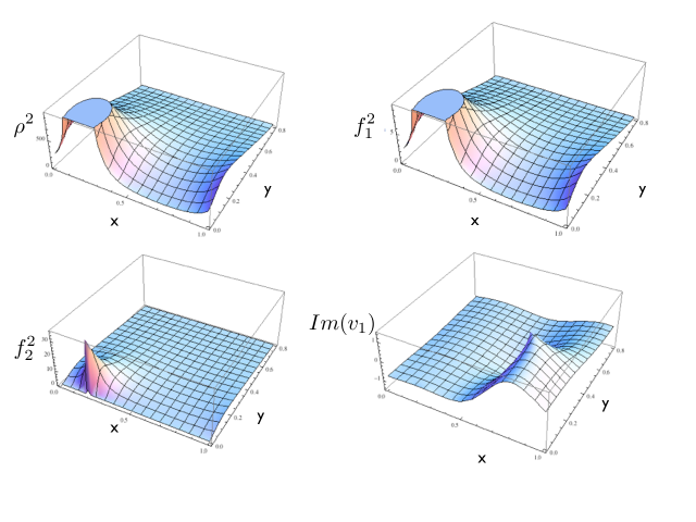
From (4) explicit expressions for the metric factors, antisymmetric tensor fields and scalars can be obtained using the formulae presented in Section 2.2. Here we present a plots for some generic values of the parameters. The metric factors are everywhere regular and the behavior of a component of the coset frame ${\rm Im}(v^{1})$ indicates the existence of a non-trivial monodromy for the scalars as discussion in Section 3.5.

4.1 General formula for the Boundary Entropy

Following [49], the boundary entropy $S_{{\scriptstyle\rm bcft}}$ is related to the ground state degeneracy $g_{{\scriptstyle\rm bcft}}$ of the degrees of freedom localized on the boundary by $S_{{\scriptstyle\rm bcft}}=\ln g_{{\scriptstyle\rm bcft}}$. For two-dimensional CFTs the boundary entropy can be extracted from the entanglement entropy $S_{A}$ of a spatial domain $A$ which is an interval of length $L$ ending at the boundary [50],

$$S_{A}={c\over 6}\ln{L\over\varepsilon}+S_{{\scriptstyle\rm bcft}}$$ (4.2)

Here $c$ is the central charge of the CFT and $\varepsilon$ is a UV cutoff. In [51, 52] a holographic prescription to calculate the entanglement entropy was developed. The entanglement entropy can be calculated as follows,

$$S_{A}={{\rm Area}(\gamma_{A})\over 4G_{N}^{(d+1)}}$$ (4.3)

where $\gamma_{A}$ is the minimal surface in the bulk which on the boundary encloses the spatial domain $A$ and $G_{N}=G_{N}^{(d+1)}$ is the Newton constant in $d+1$ dimensions. In [53], a generalization of this prescription was put forward to the case of Janus solutions which are $AdS_{2}\times S^{2}$ fibrations over a Riemann surface $\Sigma$. The minimal surface is obtained by integrating over $S^{2}$ as well as $\Sigma$ giving in our case,111111With the metric dโ€‹sฮฃ2=4โ€‹ฯ2โ€‹|dโ€‹w|2๐‘‘subscriptsuperscript๐‘ 2ฮฃ4superscript๐œŒ2superscript๐‘‘๐‘ค2ds^{2}_{\Sigma}=4\rho^{2}|dw|^{2}, the volume form on $\Sigma$ is given by $4\rho^{2}d^{2}w$ where $d^{2}w=d{\rm Re}(w)\,d{\rm Im}(w)$.

$\displaystyle S_{A}$ $\displaystyle=$ $\displaystyle{1\over 4G_{N}}\int_{\Sigma_{\varepsilon}}d^{2}w\,4\rho^{2}\,f_{2}^{2}\int_{S^{2}}\,\omega_{S^{2}}$ (4.4)
$\displaystyle=$ $\displaystyle{\pi\over G_{N}}\int_{\Sigma_{\varepsilon}}d^{2}w\,|\partial_{w}H|^{2}\left(\lambda\cdot\bar{\lambda}-2\right)$

where (2.2) was used to arrive at the second line. Here $\Sigma_{\epsilon}$ is a regularized surface obtained from $\Sigma$ by cutting out a small half-disk around the pole of $H$ located at $w=x_{1}$. A very useful formula is obtained by converting $\lambda^{A}$ into the harmonic functions $h^{A}$ using (2.17), and $\partial_{w}H$ into ${\cal N}$ using (3.15), and we have,

$\displaystyle S_{A}={4\pi\over G_{N}}\int_{\Sigma_{\varepsilon}}d^{2}w\,|{\cal N}|^{2}h^{A}h_{A}$ (4.5)

where the summation in $A$ runs over $A=1,7,8,\ldots,m+5$.

4.2 Calculation of the Boundary Entropy

Applying the general formula (4.5) for the entanglement entropy to the case of the BCFT described in (4), we find the following simplified expression,

$\displaystyle S_{A}={8\pi\over G_{N}}\Big{(}|\vec{\ell}_{1}|\,|\vec{\ell}_{2}|-\vec{\ell}_{1}\cdot\vec{\ell}_{2}\Big{)}\int_{\Sigma_{\varepsilon}}d^{2}w\,|{\cal N}|^{2}h_{0}(w-y_{1})h_{0}(w-y_{2})$ (4.6)

The dependence on the cutoff $\varepsilon$ is extracted in Appendix A.1, and we find,

$\displaystyle S_{A}={Q\cdot Q\over 8\pi^{2}G_{N}}\ln{1\over 2\pi\varepsilon}+S_{{\scriptstyle\rm bcft}}$ (4.7)

where $Q^{A}$ are the charges of the asymptotic $AdS_{3}\times S^{3}$ region, and the central charge $c$ of the bulk CFT is given by,

$\displaystyle{c\over 6}={Q\cdot Q\over 8\pi^{2}G_{N}}$ (4.8)

This central charge is in accord with the Brown-Henneaux formula derived from the radius of the asymptotic $AdS_{3}$,

$\displaystyle{c\over 6}={\ell_{3}\over 4G_{3}}\hskip 72.26999pt{1\over G_{3}}={{\rm Vol}(S^{3})\over G_{N}}$ (4.9)

where $\ell_{3}$ is the $AdS_{3}$ radius, Vol$(S^{3})$ the volume of the sphere, and $G_{3}$ is the effective 3-dimensional Newton constant. By inspection of (2.4) and (2.23), we see that $\ell_{3}=R_{n}$, and Vol$(S^{3})=2\pi^{2}R_{n}^{3}$, so that we recover

We have succeeded in analytically evaluating the integral of (4.6) for large enough modular parameter $t$. To do so, we make use of the uniform approximation of $\vartheta_{1}(w)$ and $\zeta_{0}(w)$ in the domain given in (3.1) for $\Sigma$ by the function,

$\displaystyle\vartheta_{1}(w)$ $\displaystyle=$ $\displaystyle 2e^{-\pi t/4}\sin\pi w+{\cal O}(e^{-2\pi t})$
$\displaystyle\zeta_{0}(w)$ $\displaystyle=$ $\displaystyle\pi\cot\pi w+{2\pi w\over t}+{\cal O}(e^{-2\pi t})$ (4.10)

In a lengthy calculation, which has been deferred to Appendix A.2, the finite part $S_{{\rm\scriptstyle bcft}}$ is computed analytically in $y$ and $t$ up to terms which are suppressed by powers of $e^{-\pi t}$. The final result is given by,

$\displaystyle S_{{\rm\scriptstyle bcft}}={4\pi^{2}\over G_{N}}\left(|\vec{\ell}_{1}|\,|\vec{\ell}_{2}|-\vec{\ell}_{1}\cdot\vec{\ell}_{2}\right)\left({\pi t\over 3}-{1\over 2}-{2\over\pi t}\sin^{2}\pi y+{4\over\pi^{2}t^{2}}\sin^{4}\pi y\right)+{\cal O}(e^{-\pi t})$ (4.11)

The dependence on powers in $t$, and the $y$-dependence thereof, is exact. There is some ambiguity, of course, in the splitting between the divergent part and the boundary entropy, as a change in regulator $\varepsilon$ will induce a change in $S_{{\rm\scriptstyle bcft}}$. But this change has characteristic $t$ and $y$-dependence, and may be clearly isolated.

4.3 Dependence on the scalar monodromy

For the simple BCFT discussed in the present section the additive monodromy $K^{A}$ given in (3.11) becomes

$$K^{A}={2\pi\over t}\Big{(}l_{1}^{A}+l_{2}^{A}\Big{)}$$ (4.12)

From which we can calculate the norm

$$K_{A}K^{A}={8\pi^{2}\over t^{2}}\left(|\vec{\ell}_{1}|\,|\vec{\ell}_{2}|-\vec{\ell}_{1}\cdot\vec{\ell}_{2}\right)$$ (4.13)

Where we used the fact that $\vec{\ell}_{1}{}^{A}\vec{\ell}_{1}{}_{A}=\vec{\ell}_{2}{}^{A}\vec{\ell}_{2}{}_{A}=0$. Using (4.8) and (A.11) the central charge of the BCFT can be expressed as follows

$$c={24\pi^{2}\over G_{N}}\Big{(}|\vec{\ell}_{1}|\,|\vec{\ell}_{2}|-\vec{\ell}_{1}\cdot\vec{\ell}_{2}\Big{)}|\hat{\cal N}_{0}|^{2}\hat{h}_{0}(y)^{2}$$ (4.14)

It follows from (4.13) and (4.14) that for a annulus with finite modulus $t$ setting the monodromy vector $K^{A}$ to zero implies that the central charge $c$ vanishes. This supports the interpretation of the BCFT as a near-horizon limit of a self-dual string ending on a three-brane. A vanishing monodromy implies the absence of a three-brane and consequently the self-dual string has nowhere to end. In our supergravity solution this is reflected by the fact that the a solution dual to a BCFT with $N=1$ and vanishing $K^{A}$ cannot be regular. On the other hand, solutions with $N>1$ corresponding to interfaces or junctions of self-dual strings exist with vanishing monodromy $K^{A}$.

4.4 Degeneration of the annulus solution

Next, we derive the asymptotic behavior of the annulus solutions of Sections 3 and 4 for large $t$, namely when the inner boundary component is shrunk. The nature of this degeneration will help in understanding the connection with other solutions, such as the $AdS_{2}$-funnel introduced in [31, 45]. In taking this degeneration limit, we shall keep fixed the physical data in the asymptotic regions, namely the charges and values of the un-attracted scalars. We should expect to find the disk solution of Section 2.4 to leading order, as well as physically interesting sub-leading corrections to the disk solution.

The approximations to be used here are the ones of (4.2) that allowed us to derive the boundary entropy in a uniform expansion valid exactly in $t,y$, up to exponential corrections of the form $e^{-\pi t}$. To connect the limiting solutions with those of the disk, it will be convenient to map the degenerated annulus onto the upper half-plane (in terms of which the disk solution was previously formulated) by introducing the following change of coordinates,

$\displaystyle z=-\cot\pi w\,\qquad$ $\displaystyle\quad u_{n}=-\cot\pi x_{n}\quad$ $\displaystyle\qquad v_{p}=-\cot\pi y_{p}$
$\displaystyle z^{\prime}=-\cot\pi w^{\prime}\qquad$ $\displaystyle\quad u^{\prime}_{n^{\prime}}=-\cot\pi x^{\prime}_{n^{\prime}}\quad$ $\displaystyle\qquad v^{\prime}_{p^{\prime}}=-\cot\pi y^{\prime}_{p^{\prime}}$ (4.15)

Note that $u_{n},u^{\prime}_{n^{\prime}},v_{p}$, and $v^{\prime}_{p^{\prime}}$ are real. The different regions of the annulus may be described by the following coordinate regions,

$\displaystyle\Sigma_{\rm lower}$ $\displaystyle=$ $\displaystyle\Big{\{}0\leq{\rm Im}(w)\ll t/2\Big{\}}$
$\displaystyle\Sigma_{\rm center}$ $\displaystyle=$ $\displaystyle\Big{\{}|{\rm Im}(w)-t/2)|\ll t/2\Big{\}}$
$\displaystyle\Sigma_{\rm upper}$ $\displaystyle=$ $\displaystyle\Big{\{}0\leq{\rm Im}(w^{\prime})\ll t/2\Big{\}}$ (4.16)

Suitable coordinates in each region are respectively $z$, $w$, and $z^{\prime}$.

Refer to caption
Figure 8: The regions $\Sigma_{\rm lower}$, $\Sigma_{\rm center}$, and $\Sigma_{\rm upper}$.

The basic meromorphic functions then take the following form,

$\displaystyle\zeta_{0}(w-x)=\pi{1+u^{2}\over z-u}+{2\pi(w-x)\over t}+\pi u$ (4.17)

Here, we have not converted the term in $w-x$ because its contribution will dominate in the region $\Sigma_{\rm center}$ where $w$ is a suitable coordinate. The expressions for the basic harmonic and holomorphic functions are then given by,

$\displaystyle H$ $\displaystyle=$ $\displaystyle-2\,{\rm Im}\sum_{n=1}^{N}c_{n}\left(\pi{1+u_{n}^{2}\over z-u_{n}}+{2\pi w\over t}\right)-2\,{\rm Im}\sum_{n^{\prime}=1}^{N^{\prime}}c^{\prime}_{n^{\prime}}\left(\pi{1+u_{n^{\prime}}^{\prime 2}\over z^{\prime}+u^{\prime}_{n^{\prime}}}+{2\pi w^{\prime}\over t}\right)$ (4.18)
$\displaystyle L^{A}$ $\displaystyle=$ $\displaystyle L_{0}^{A}+\sum_{p=1}^{P}\ell^{A}_{p}\left(\pi{1+v_{p}^{2}\over z-v_{p}}+{2\pi w\over t}+\pi v_{p}\right)+\sum_{p^{\prime}=1}^{P^{\prime}}\ell^{\prime A}_{p^{\prime}}\left(\pi{1+v_{p^{\prime}}^{\prime 2}\over z^{\prime}+v^{\prime}_{p^{\prime}}}+{2\pi w^{\prime}\over t}-\pi v^{\prime}_{p^{\prime}}\right)$

For large $t$, the behavior in the different regions is as follows. In $\Sigma_{\rm lower}$ the terms in $1/t$ and in $z^{\prime}$ may be neglected to leading approximation. In particular, we have $z^{\prime}=i+{\cal O}(e^{-\pi t})$ in this region, so that the contributions of the $z^{\prime}$ terms to $H$ and $L_{0}^{A}$ vanish to this order. Thus, in the region $\Sigma_{\rm lower}$ we have,

$\displaystyle H=-2\pi\,{\rm Im}\sum_{n=1}^{N}c_{n}{1+u_{n}^{2}\over z-u_{n}}\hskip 72.26999ptL^{A}=L_{0}^{A}+\pi\sum_{p=1}^{P}\ell^{A}_{p}{1+v_{p}^{2}\over z-v_{p}}$ (4.19)

up to corrections suppressed by $e^{-\pi t}$. Similarly, in the region $\Sigma_{\rm upper}$ we retain only the terms in $z^{\prime}$. The corresponding expressions for $H$ and $L^{A}$ may be read off from (4.18).

It remains to determine the behavior of the solution in the region $\Sigma_{\rm center}$. It will be convenient to parametrize $w=\alpha+it\beta/2$, so that the region $\Sigma_{\rm center}$ corresponds to $0\leq\alpha<1$ and $|\beta-1/2|\ll 1$. In this regime, we have $z=i+{\cal O}(e^{-\pi t/2})$ as well as $z^{\prime}=i+{\cal O}(e^{-\pi t/2})$, so that all terms involving $z$ and $z^{\prime}$ cancel out of $H$ and $L^{A}$ in (4.18) to this order, and we are left with,

$\displaystyle H$ $\displaystyle=$ $\displaystyle(1-\beta){\cal C}+\beta{\cal C}^{\prime}$
$\displaystyle L^{A}$ $\displaystyle=$ $\displaystyle L_{0}^{A}-iK_{0}^{A}+\left(\alpha+{it\over 4}(2\beta-1)\right)K^{A}$ (4.20)

where we have defined $K^{A}$ as the monodromy in (3.11), and the remaining quantities by,

$\displaystyle{\cal C}=2\pi\sum_{n=1}^{N}c_{n}\hskip 43.36243pt{\cal C}^{\prime}=2\pi\sum_{n^{\prime}=1}^{N^{\prime}}c^{\prime}_{n^{\prime}}\hskip 57.81621ptK_{0}^{A}={\pi\over 2}\left(\sum_{p=1}^{P}\ell^{A}_{p}+\sum_{p^{\prime}=1}^{P^{\prime}}\ell^{\prime A}_{p^{\prime}}\right)$ (4.21)

We see that near $\beta=1/2$, $H$ and $L^{6}$ are approximately non-zero constants, while the other $L^{A}$ are linear in $w-\tau/4$. Thus, the geometry is that of the product space,

$\displaystyle AdS_{2}\times S^{2}\times S^{1}\times I_{\beta}$ (4.22)

where $I_{\beta}$ is the interval in $\beta$ for the region $\Sigma_{\rm center}$. Through its dependence on $\alpha$, the functions $L^{A}$ retain their monodromy, thus transferring monodromy also to the scalars. This geometry is the realization of the funnel, but now supplemented with the necessary monodromy to make funnels on the asymptotic disks possible with non-zero charge transfers.

5 Half-BPS string-junction solutions at higher genus

The set-up for string-junction solutions in Type IIB in the presence of multiple boundary components was given in [30] for the special case of $SO(2,2)$ holonomy and genus 0. In the present section, we shall relax both restrictions, and construct string-junction solutions with general $SO(2,m)$ holonomy, with an arbitrary number of boundary components $\nu$, and arbitrary genus $g$. We begin by reviewing some standard results on higher genus bordered surfaces, discussed generally in [48, 54].

5.1 Higher genus set-up with boundary components

Consider an orientable Riemann surface $\Sigma$ of genus $g$ with $\nu$ boundary components. As usual, we construct functions and forms on $\Sigma$ in terms of functions and forms on the double cover Riemann surface $\hat{\Sigma}$, restricted under the anti-conformal involution $\phi$. The boundary $\partial\Sigma$ of $\Sigma$ is fixed under $\phi$, so that $\phi(\partial\Sigma)=\partial\Sigma$, and we may view $\Sigma$ as the quotient $\Sigma=\hat{\Sigma}/\phi$. The genus $\hat{g}$ of $\hat{\Sigma}$ is related to $g$ and $\nu$ by,

$\displaystyle\hat{g}=2g+\nu-1$ (5.1)

This construction is depicted schematically in Figure 9 for the case $g=2$ and $\nu=3$.

Refer to caption
Figure 9: The Riemann surface $\Sigma$ of genus $g=2$ with $\nu=3$ boundary components $A_{3},\,A_{4},\,A_{5}$, and its double compact Riemann surface $\hat{\Sigma}=\Sigma\cup\phi(\Sigma)$ of genus $\hat{g}=6$.

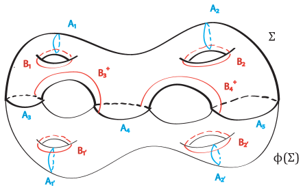
It will be useful to sort homology cycles, and their dual holomorphic 1-forms, according to their behavior under the involution $\phi$. Our labeling generalizes the one indicated in Figure 9,

$2g$ cycles belonging to $\Sigma$ $\displaystyle A_{I},\,B_{I},\hskip 36.135ptI=1,\ldots,g$ (5.2)
$2g$ cycles conjugate under $\phi$ $\displaystyle A_{I^{\prime}},\,B_{I^{\prime}}$
$\nu$ boundary cycles for $\partial\Sigma$ $\displaystyle A_{i},\hskip 36.135pti=g+1,\ldots,g+\nu$
$\nu-1$ conjugate cycles for $\partial\Sigma$ $\displaystyle B_{i},\hskip 36.135pti=g+1,\ldots,g+\nu-1$

Note that the boundary cycle $A_{g+\nu}$ is homologically dependent upon the other above cycles. The basis of cycles, and their orientations, may be chosen such that,

$\displaystyle A_{I^{\prime}}=+\phi(A_{I})$ $\displaystyle\phi(A_{i})=+A_{i}$
$\displaystyle B_{I^{\prime}}=-\phi(B_{I})$ $\displaystyle\phi(B_{i})=-B_{i}$ (5.3)

Throughout, indices $I$ and $i$ will be running over the ranges defined in (5.2). The corresponding holomorphic differentials will be denoted by $\omega_{I},\omega_{I^{\prime}}$, and $\omega_{i}$, and may be canonically normalized by the following relations,

$\displaystyle\oint_{A_{I}}\omega_{J}=\oint_{A_{I^{\prime}}}\omega_{J^{\prime}}=\delta_{IJ}\hskip 72.26999pt\oint_{A_{i}}\omega_{j}=\delta_{ij}$ (5.4)

all other integrals over $A$-cycles being zero. As a result of (5.1), we then have the following involution relations for the holomorphic differentials,

$\displaystyle\phi^{*}(\omega_{I})$ $\displaystyle=$ $\displaystyle\bar{\omega}_{I^{\prime}}$
$\displaystyle\phi^{*}(\omega_{I^{\prime}})$ $\displaystyle=$ $\displaystyle\bar{\omega}_{I}$
$\displaystyle\phi^{*}(\omega_{i})$ $\displaystyle=$ $\displaystyle\bar{\omega}_{i}$ (5.5)

where $\phi^{*}$ is the pull-back of $\phi$ to differential forms. The period matrix of $\hat{\Sigma}$ is defined by,

$\displaystyle\oint_{B_{\hat{I}}}\omega_{\hat{J}}=\Omega_{\hat{I}\hat{J}}$ (5.6)

where we make use of the composite indices $\hat{I}=(I,I^{\prime},i)$ and $\hat{J}=(J,J^{\prime},j)$. The matrix is symmetric $\Omega_{\hat{J}\hat{I}}=\Omega_{\hat{I}\hat{J}}$, and has positive definite imaginary part ${\rm Im}(\Omega)>0$. As a result of the involution relations (5.4), there exist further relations between the entries of $\Omega_{\hat{I}\hat{J}}$, deduced from the following integral relations,

$\displaystyle\Omega_{ij}=\oint_{B_{i}}\omega_{j}$ $\displaystyle=$ $\displaystyle-\oint_{\phi(B_{i})}\phi^{*}(\bar{\omega}_{j})=-\oint_{B_{i}}\bar{\omega}_{j}=-\bar{\Omega}_{ij}$
$\displaystyle\Omega_{iJ^{\prime}}=\oint_{B_{i}}\omega_{J^{\prime}}$ $\displaystyle=$ $\displaystyle-\oint_{\phi(B_{i})}\phi^{*}(\bar{\omega}_{J})=-\oint_{B_{i}}\bar{\omega}_{J}=-\bar{\Omega}_{iJ}$
$\displaystyle\Omega_{I^{\prime}J^{\prime}}=\oint_{B_{I^{\prime}}}\omega_{J^{\prime}}$ $\displaystyle=$ $\displaystyle-\oint_{\phi(B_{I})}\phi^{*}(\bar{\omega}_{J})=-\oint_{B_{I}}\bar{\omega}_{J}=-\bar{\Omega}_{IJ}$
$\displaystyle\Omega_{I^{\prime}J}=\oint_{B_{I^{\prime}}}\omega_{J}$ $\displaystyle=$ $\displaystyle-\oint_{\phi(B_{I})}\phi^{*}(\bar{\omega}_{J^{\prime}})=-\oint_{B_{I}}\bar{\omega}_{J^{\prime}}=-\bar{\Omega}_{IJ^{\prime}}$ (5.7)

Thus, $\Omega$ takes on the following block form, where the indices run over $\hat{I}=(I,I^{\prime},i)$,

$\displaystyle\bar{\Omega}=-{\cal K}\Omega{\cal K}^{t}\hskip 57.81621pt{\cal K}=\left(\matrix{0&I_{g}&0\cr I_{g}&0&0\cr 0&0&I_{\nu-1}\cr}\right)$ (5.8)

where $I_{g}$ and $I_{\nu-1}$ are the identity matrices respectively in dimensions $g$ and $\nu-1$.

5.2 Construction of the harmonic function $h_{0}$

As is familiar from the case of the annulus, the harmonic functions $H$ and $h^{A}$ may all be built up out of a single type of elementary harmonic function $h_{0}(w|x)$ which has a single simple pole on the boundary at $x\in\partial\Sigma$. In terms of meromorphic functions $Z_{0}$ we have,

$\displaystyle h_{0}(w|x)=iZ_{0}(w|x,q)-iZ_{0}(\phi(w)|x,q)$ (5.9)

where $Z_{0}(w|x_{0},q)$ is an Abelian integral of the second kind, with a single simple pole at $x$. The auxiliary point $q$ will drop out of $h_{0}$ provided $q\in\partial\Sigma$. A convenient building block for Abelian integrals of the second kind is the prime form $E(z,w)$ for the surface $\hat{\Sigma}$, as well as the holomorphic Abelian 1-forms $\omega_{\hat{I}}$ on $\hat{\Sigma}$. In terms of those, we have,

$\displaystyle Z_{0}(w|x,q)=\int_{q}^{w}dy\left(\partial_{x}\partial_{y}\ln E(x,y)+\sum_{\hat{I}}\alpha_{\hat{I}}(x)\omega_{\hat{I}}(y)\right)$ (5.10)

where the complex 1-forms $\alpha_{\hat{I}}(x)$ remain to be determined. To do so, we use the conditions:

  1. 1.

    $h_{0}$ must be single-valued around the cycles $A_{I}$, $B_{I}$, $A_{I^{\prime}}$, and $B_{I^{\prime}}$ for $I=1,\ldots,g$;

  2. 2.

    $h_{0}$ must vanish along the cycles $A_{i}$ for $i=g+1,\ldots,g+\nu$;

  3. 3.

    $h_{0}$ must be positive inside $\Sigma$, a condition which will follow from the above requirements.

We begin by implementing condition 1. on the cycles $A_{I}$ and $A_{I^{\prime}}$. The first term in (5.10) has trivial monodromy under all $A$-cycles. Computing the monodromy under general $A_{\hat{I}}$-cycles, the contribution of the second term of Abelian integrals of the first kind gives,

$\displaystyle Z_{0}(w+A_{\hat{I}}|x,q)=Z_{0}(w|x,q)+\alpha_{\hat{I}}(x)$ (5.11)

Single-valuedness of $h_{0}$ under the cycles $A_{I}$ and $A_{I^{\prime}}$ thus requires $\alpha_{I},\alpha_{I^{\prime}}\in{\bf R}$. Next, we implement condition 1. on cycles $B_{I}$ and $B_{I^{\prime}}$. This time both terms in (5.10) contribute to the monodromy, and we use the well-known relation,

$\displaystyle\oint_{B_{\hat{I}}}dy\,\partial_{x}\partial_{y}\ln E(x,y)=2\pi i\omega_{\hat{I}}(x)$ (5.12)

We find,

$\displaystyle Z_{0}(w+B_{\hat{I}}|x,q)=Z_{0}(w|x,q)+2\pi i\omega_{\hat{I}}(x)+\sum_{\hat{J}}\alpha_{\hat{J}}(x)\Omega_{\hat{I}\hat{J}}$ (5.13)

Since $\phi^{*}(\omega_{\hat{I}})=\bar{\omega}_{\hat{I}}$, and $\phi(x)=x$, single-valuedness of $h_{0}$ around the cycles $B_{I}$ and $B_{I^{\prime}}$ requires the following relations,

$\displaystyle 0$ $\displaystyle=$ $\displaystyle-2\pi\omega_{I}(x)-2\pi\bar{\omega}_{I}(x)+i\sum_{\hat{J}}\alpha_{\hat{J}}(x)\Omega_{I\hat{J}}-i\sum_{\hat{J}}\bar{\alpha}_{\hat{J}}(x)\bar{\Omega}_{I\hat{J}}$
$\displaystyle 0$ $\displaystyle=$ $\displaystyle-2\pi\omega_{I^{\prime}}(x)-2\pi\bar{\omega}_{I^{\prime}}(x)+i\sum_{\hat{J}}\alpha_{\hat{J}}(x)\Omega_{I^{\prime}\hat{J}}-i\sum_{\hat{J}}\bar{\alpha}_{\hat{J}}(x)\bar{\Omega}_{I^{\prime}\hat{J}}$ (5.14)

Before solving these equations, we first derive the consequences of condition 2.

To implement condition 2, we make use of the conjugation property of the prime form,

$\displaystyle\phi^{*}E(x,y)=\overline{E(x,y)}$ (5.15)

If $x,y$ belong to the same boundary component, then this equation implies that $E(x,y)$ is real. If, however, $x,y$ belong to different boundary components, then $E(x,y)$ will not in general be real. We begin by considering the case where $x$ belongs to a definite boundary component, which we take to be $A_{g+\nu}$. Since $h_{0}$ does not depend on $q$, we shall assume that also $q\in A_{g+\nu}$. As a result of (5.15), we see that $Z_{0}(w|x,q)$ is real when $w\in A_{g+\nu}$, so that

$\displaystyle h_{0}(w|x)=0\hskip 72.26999pt\hbox{when}~{}w,x\in A_{g+\nu}$ (5.16)

The same argument could have been made for $w,x$ belonging both to any given one of the $A_{i}$-cycles of $\partial\Sigma$, but the issue at hand here is whether the choice can be made consistently simultaneously on all the cycles $A_{i}$. Two different $A_{i}$ cycles are separated by a sum of half $B_{i}$-cycles. Thus, it suffices to investigate the relation between $h_{0}$ evaluated on points $w$ and $w^{\prime}$ which differ by a half-cycle $B_{i}^{+}$. To this end, we calculate,

$\displaystyle h_{0}(w^{\prime}|x)-h_{0}(w|x)$ $\displaystyle=$ $\displaystyle i\left(\int_{B_{i}^{+}}-\int_{B_{i}^{-}}\right)\bigg{(}dy\,\partial_{y}\partial_{x}\ln E(x,y)+\sum_{\hat{J}}\alpha_{\hat{J}}(x)\omega_{\hat{J}}\bigg{)}$ (5.17)
$\displaystyle=$ $\displaystyle i\oint_{B_{i}}\bigg{(}dy\,\partial_{y}\partial_{x}\ln E(x,y)+\sum_{\hat{J}}\alpha_{\hat{J}}(x)\omega_{\hat{J}}\bigg{)}$

The integral may be carried out, and the result may be decomposed as follows,

$\displaystyle h_{0}(w^{\prime}|x)-h_{0}(w|x)=-2\pi\omega_{i}(x)+i\sum_{J}\alpha_{J}(x)\Omega_{iJ}+i\sum_{J^{\prime}}\alpha_{J^{\prime}}(x)\Omega_{iJ^{\prime}}+i\sum_{j}\alpha_{j}(x)\Omega_{ij}$ (5.18)

The left side is real by construction, requiring also the right side to be real. Clearly, $\omega_{i}(x)$ is real for $x\in\partial\Sigma$. Since $\Omega_{ij}$ is purely imaginary, $\alpha_{i}$ must be real. Thus, all coefficients $\alpha_{\hat{I}}$ must be real. From the second line in (5.1), we have $\Omega_{iJ^{\prime}}=-\bar{\Omega}_{iJ}$, from which we see that the remaining terms in (5.18) will be real provided we require also $\alpha_{J^{\prime}}=\alpha_{J}$. Setting $h_{0}(w^{\prime}|x)=h_{0}(w|x)$ for all $B_{i}$-cycles will precisely enforce all the required Dirichlet boundary conditions. Assembling these conditions with those derived in (5.2), and using the reality of $\alpha_{\hat{I}}$, then gives the following set of conditions,

$\displaystyle\sum_{\hat{J}}{\rm Im}\left(\Omega_{\hat{I}\hat{J}}\right)\alpha_{\hat{J}}(x)=-\pi\omega_{\hat{I}}(x)-\pi\bar{\omega}_{\hat{I}}(x)$ (5.19)

The matrix ${\rm Im}(\Omega)$ is invertible, and may be used to solve uniquely for $\alpha_{\hat{I}}$. To complete the determination of the harmonic function $h_{0}$, it remains to establish its positivity.

5.3 Positivity of $h_{0}(w|x)$

For the construction of $H$ and $h^{A}$ to work, the harmonic function $h_{0}(w|x)$ must be positive. Note that the electrostatics interpretation of $h_{0}$ is that of the electric potential produced by a point-like electric dipole with unit strength, placed at the boundary point $x$, and with positive polarity facing inward into $\Sigma$, while maintaining the boundary grounded. It is intuitively clear that the potential inside $\Sigma$ must then always be positive. A mathematical proof of the same fact may be given by using the Minimum-Maximum Theorem for harmonic functions. It states that if $h_{0}$ is harmonic, then on every compact subspace $K$ (of whatever manifold on which the harmonic function lives), the function $h_{0}$ will attain its minimum and its maximum on the boundary $\partial K$ of $K$.

To apply the theorem here, we consider any subspace $\Sigma_{\varepsilon}$ of $\Sigma$ which avoids the singularity, and on which $h_{0}$ is a smooth harmonic function. For a general choice of $\Sigma_{\varepsilon}$, the values of $h_{0}$ along $\partial\Sigma_{\varepsilon}$ are unknown to us. A useful choice for $\Sigma_{\varepsilon}$ is obtained by removing from $\Sigma$ a small half-disk of radius $\varepsilon$ around the pole at $x$. The boundary of $\Sigma_{\varepsilon}$ now consists of the boundary of $\Sigma$ with a small half-circle around the pole replacing the line segment through the pole. On the boundary of $\Sigma$ part, $h_{0}$ vanishes, while on the half-circle part we can compute the value of $h_{0}$ approximately for sufficiently small $\varepsilon$ since the behavior there is dominated by the pole. But near the pole $h_{0}$ is positive; hence $h_{0}$ must be positive throughout $\Sigma$.

5.4 Construction of $H$, $h^{A}$, and $L^{A}$

Transcribing the Type IIB solution with holonomy $SO(2,2)$ and genus 0 to the case of the 6-dimensional supergravity, extending to full $SO(2,m)$ holonomy, as well as generalizing to arbitrary genus $g$, we see that the structure in light-cone variables is very similar to the one derived for the annulus. Indeed, the fundamental functions are given by,

$\displaystyle H(w)$ $\displaystyle=$ $\displaystyle\sum_{n=1}^{N}c_{n}\,h_{0}(w|x_{n})$
$\displaystyle h^{A}(w)$ $\displaystyle=$ $\displaystyle-{1\over 2}\sum_{p=1}^{P}\ell^{A}_{p}\,h_{0}(w|y_{p})$
$\displaystyle L^{A}(w)$ $\displaystyle=$ $\displaystyle L^{A}_{0}+\sum_{p=1}^{P}\ell^{A}_{p}Z_{0}(w|y_{p},q)$ (5.20)

for $A=1,6,7,\ldots,m+5$. The functions $h_{0}$ and $Z_{0}$ were constructed in the preceding sections. The points $x_{n}$ and $y_{p}$ lie on the boundary $\partial\Sigma$, and will in general be distributed across the different boundary components. The above notation subsumes the one used for the annulus, so that the points $x_{n}$ and $x^{\prime}_{n^{\prime}}$ of the annulus are collected here into a single notation of points $x_{n}$, and similarly for the points $y_{p}$. The residues $c_{n}$ and $\ell^{A}_{p}$ are real, and we have $c_{n}>0$. Finally, the harmonic function $h_{0}$ may be expressed in terms of a meromorphic Abelian integral $Z_{0}$ of the second kind, as was done in (5.9).

5.5 Single-valuedness of $L^{6}$

In the light-cone parametrization of the solutions, it is essential that the light-cone function $\lambda^{-}=1/(\sqrt{2}L^{6})$, and thus $L^{6}$ be single-valued on $\Sigma$. This means absence of monodromies around the cycles $A_{I},B_{I},A_{I^{\prime}},B_{I^{\prime}}$, as well as the boundary cycles $A_{i}$. Since the boundary cycle $A_{g+\nu}$ is homologically a linear combination of $A_{i}$-cycles, no condition on $A_{g+\nu}$ needs to be imposed separately. Making use of the monodromy equations (5.11) and (5.13), as well as condition (5.19), we have the following monodromies for $Z_{0}$,

$\displaystyle Z_{0}(w+A_{\hat{I}}|x,q)$ $\displaystyle=$ $\displaystyle Z_{0}(w|x,q)+\alpha_{\hat{I}}(x)$
$\displaystyle Z_{0}(w+B_{\hat{I}}|x,q)$ $\displaystyle=$ $\displaystyle Z_{0}(w|x,q)+\beta_{\hat{I}}(x)$ (5.21)

where $\alpha_{\hat{I}}$ and $\beta_{\hat{I}}$ are real, and $\beta_{\hat{I}}$ is given by,

$\displaystyle\beta_{\hat{I}}(x)=i\pi\Big{(}\omega_{\hat{I}}(x)-\bar{\omega}_{\hat{I}}(x)\Big{)}+{1\over 2}\sum_{\hat{J}}\left(\Omega_{\hat{I}\hat{J}}+\bar{\Omega}_{\hat{I}\hat{J}}\right)\alpha_{\hat{J}}(x)$ (5.22)

It is immediate from the relations $\alpha_{I^{\prime}}=\alpha_{I}$ and (5.1) that we have,

$\displaystyle\beta_{I^{\prime}}(x)=-\beta_{I}(x)\hskip 72.26999pt\beta_{i}(x)=0$ (5.23)

The absence of monodromy for $A_{I}$- and $B_{I}$-cycles implies the absence of monodromy for $A_{I^{\prime}}$- and $B_{I^{\prime}}$-cycles, since we have $\alpha_{I^{\prime}}=\alpha_{I}$ and $\beta_{I^{\prime}}(x)=-\beta_{I}(x)$. Together with the absence of monodromy around $A_{i}$-cycles, these conditions restrict the residues $\ell^{6}_{p}$ as follows,

$\displaystyle\sum_{p=1}^{P}\ell^{6}_{p}\,\alpha_{I}(y_{p})=\sum_{p=1}^{P}\ell^{6}_{p}\,\beta_{I}(y_{p})=\sum_{p=1}^{P}\ell^{6}_{p}\,\alpha_{i}(y_{p})=0$ (5.24)

which must hold for all $I=1,\ldots,g$, and $i=g+1,\ldots,g+\nu-1$.

As was the case for the annulus, an alternative construction for $L^{6}$ may be given in terms of a multiplicative formula, by expressing the 1-form ${\cal N}(w)=\partial_{w}H/L^{6}$ in terms of the prime form $E(z,w)$ and the holomorphic form $\sigma(z)$. The former has weight $(-1/2,0)$ in $z$ and $w$, and the latter has weight $(\hat{g}/2,0)$ in $z$. Both were introduced by Fay in [54], and reviewed in [30]. Here, we shall only need the following properties. Both $E(z,w)$ and $\sigma(v)$ are free of monodromy around $A_{\hat{I}}$-cycles, and have the following monodromy around $B_{\hat{I}}$-cycles,

$\displaystyle E(z+B_{\hat{I}},w)$ $\displaystyle=$ $\displaystyle-E(z,w)\exp\Big{\{}-i\pi\Omega_{\hat{I}\hat{I}}-2\pi i\varphi_{\hat{I}}(z)+2\pi i\varphi_{\hat{I}}(w)\Big{\}}$
$\displaystyle\sigma(z+B_{\hat{I}})^{2}$ $\displaystyle=$ $\displaystyle\sigma(z)^{2}\exp\Big{\{}2\pi i(\hat{g}-1)\Omega_{\hat{I}\hat{I}}-4\pi i\Delta_{\hat{I}}+4\pi i(\hat{g}-1)\varphi_{\hat{I}}(z)\Big{\}}$ (5.25)

where $\varphi_{\hat{I}}:\hat{\Sigma}\to{\bf C}^{\hat{g}}/\Lambda$ is the Abel map, and $\Delta$ the Riemann vector, defined by,

ฯ†I^โ€‹(z)=โˆซz0zฯ‰I^โ€‹ฮ”I^=12โˆ’12โ€‹ฮฉI^โ€‹I^+โˆ‘J^โ‰ I^โˆฎAJ^ฯ‰J^โ€‹ฯ†I^subscript๐œ‘^๐ผ๐‘งsuperscriptsubscriptsubscript๐‘ง0๐‘งsubscript๐œ”^๐ผsubscriptฮ”^๐ผ1212subscriptฮฉ^๐ผ^๐ผsubscript^๐ฝ^๐ผsubscriptcontour-integralsubscript๐ด^๐ฝsubscript๐œ”^๐ฝsubscript๐œ‘^๐ผ\displaystyle\varphi_{\hat{I}}(z)=\int_{z_{0}}^{z}\omega_{\hat{I}}\hskip 72.26999pt\Delta_{\hat{I}}={1\over 2}-{1\over 2}\Omega_{\hat{I}\hat{I}}+\sum_{\hat{J}\not=\hat{I}}\oint_{A_{\hat{J}}}\omega_{\hat{J}}\,\varphi_{\hat{I}} (5.26)

The lattice $\Lambda$ is generated by $(I,\Omega)$, The formula for $L^{6}$ is then built up as follows,

$\displaystyle{\cal N}(w)={\cal N}_{0}e^{-2\pi i\theta^{t}\varphi(w)}{\prod_{p=1}^{P}E(w,y_{p})\over\prod_{n=1}^{N}E(w,x_{n})^{2}}\sigma(w)^{2}$ (5.27)

It is readily verified that ${\cal N}$, thus constructed, is automatically a form of weight $(1,0)$ in $w$, and has the correct poles and zeros. Absence of monodromy around $A$-cycles requires that all the entries of the column vector $\theta$ be integers. As for the annulus, we shall assume that ${\cal N}$ is single-valued on $\hat{\Sigma}$. The Riemann-Roch theorem then implies the following relation between the number of poles, zeros, and the genus,

$\displaystyle P-2N=2\hat{g}-2$ (5.28)

Absence of monodromy of ${\cal N}$ then reduces to the conditions,

$\displaystyle\sum_{p=1}^{P}\varphi_{\hat{I}}(y_{p})-2\sum_{n=1}^{N}\varphi_{\hat{I}}(x_{n})-2\Delta_{\hat{I}}=\theta^{\prime}_{\hat{I}}+\sum_{\hat{I}}\Omega_{\hat{I}\hat{J}}\theta_{\hat{J}}$ (5.29)

where $\theta_{\hat{I}}$ and $\theta^{\prime}_{\hat{I}}$ are integers. Since the right side belongs to $\Lambda$, this condition is just the usual canonical divisor condition for meromorphic 1-forms.

5.6 Reality of $L^{6}$ on all boundary components

By construction, ${\cal N}(w)$ is single-valued on $\Sigma$, including around the homology cycles $A_{I},B_{I}$ and the boundary cycles $A_{i}$. It remains to ensure that $L^{6}(w)$, as defined by $L^{6}(w)=\partial_{w}H/{\cal N}(w)$, is real on all boundary components. This in turn requires that ${\cal N}(w)$ should be purely imaginary on all boundary components. Since ${\cal N}(w)$ is defined only up to a multiplicative complex constant ${\cal N}_{0}$, it will suffice to show that,

  1. 1.

    The phase of ${\cal N}(w)$ is constant (independent of $w$) on each boundary component.

  2. 2.

    The constant phases of ${\cal N}(w)$ on different boundary components are the same.

It will then follow that the phase of the overall multiplicative constant ${\cal N}_{0}$ may be chosen so that ${\cal N}(w)$ is purely imaginary on all boundary components.

5.6.1 The phases of the prime form on boundary points

We begin by calculating the phases of the prime form $E(u,v)$, evaluated between points $u,v$ on the boundary of $\Sigma$. When $u,v$ belong to the same boundary component $E(u,v)$ is real. Next, we assume that $u\in A_{i}$ and $v\in A_{i+1}$. One may represent the point $v$ as the image under a half $B_{i}$-period of a point $v^{\prime}$ on $A_{i}$, namely $v=v^{\prime}+B_{i}^{+}$ with $B^{+}_{i}\subset\Sigma$. We then have,

$\displaystyle{E(u,v)\over E(u,v)^{*}}={E(u,v^{\prime}+B_{i}^{+})\over E(u,v^{\prime}+B_{i}^{-})}={E(u,v)\over E(u,v-B_{i})}$ (5.30)

Using formula (5.5) for the $B_{i}$-cycle shift of the prime form, we find,

$\displaystyle{E(u,v)\over E(u,v)^{*}}=-\exp\left\{i\pi\Omega_{ii}-2\pi i\int^{v}_{u}\omega_{i}\right\}$ (5.31)

where the integral is taking along a curve inside $\Sigma$ which is homologous to a sum of half-periods $B_{i}^{+}$. Despite its appearance, the argument of the exponential in (5.31) is purely imaginary. To see this, we take its real part, which is found to be,

$\displaystyle i\pi\Omega_{ii}-\pi i\int^{v}_{u}\omega_{i}+\pi i\overline{\int^{v}_{u}\omega_{i}}=i\pi\Omega_{ii}-\pi i\oint_{B_{i}}\omega_{i}=0$ (5.32)

Thus, we may write instead of (5.31) a simpler formula in which this property is manifest,

$\displaystyle{E(u,v)\over E(u,v)^{*}}=-\exp\left\{-2\pi i\,{\rm Re}\int^{v}_{u}\omega_{i}\right\}$ (5.33)

Recall that this result was derived when $u\in A_{i}$ and $v\in A_{i+1}$.

Next, we proceed to the general case with $u\in A_{i}$ and $v\in A_{j}$. In view of the property $E(u,v)=-E(v,u)$, we may choose $g+1\leq i<j\leq g+\nu$ without loss of generality. To compute the phase of $E(u,v)$, we proceed analogously to the earlier case, and we have,

$\displaystyle{E(u,v)\over E(u,v)^{*}}={E(u,v)\over E(u,v-\sum_{k}c_{i,j}^{k}B_{k})}$ (5.34)

where we have defined the following symbol,

$\displaystyle c_{i,j}^{k}=\left\{\matrix{+1&\hbox{if}&i\leq k<j\cr-1&\hbox{if}&j\leq k<i\cr 0&&\hbox{otherwise}\cr}\right.$ (5.35)

The repeated index $k$ must be summed over the range $g+1\leq k\leq g+\nu-1$. Immediate, and useful, properties of the symbol $c_{i,j}^{k}$ are the following relations,

$\displaystyle c^{k}_{j,i}+c^{k}_{i,j}$ $\displaystyle=$ $\displaystyle 0$
$\displaystyle c_{i+1,j}^{k}-c_{i,j}^{k}$ $\displaystyle=$ $\displaystyle\delta_{ik}$ (5.36)

To compute the denominator of (5.34), we iterate $j-i$ times the formula (5.30), and obtain the following generalization of (5.33),

$\displaystyle{E(u,v)\over E(u,v)^{*}}=(-)^{i-j}\exp\left\{-2\pi i\,\sum_{k}c_{i,j}^{k}\Big{(}{\rm Re}\,\varphi_{k}(v)-{\rm Re}\,\varphi_{k}(u)\right)\Big{\}}$ (5.37)

The definition of the symbol $c_{i,j}^{k}$ was adopted in (5.35) so that formula (5.37) holds for $u\in A_{i}$ and $v\in A_{j}$, without any restriction on the ordering of the indices $i,j$.

5.6.2 The phase of $\sigma$ on boundary points

We make use of the following representation of $\sigma$ in terms of $\vartheta$-functions [48, 54],

$\displaystyle{\sigma(u)\over\sigma(u_{0})}={\vartheta(\varphi(u)-\sum_{\alpha}\varphi(q_{\alpha})+\Delta)\over\vartheta(\varphi(u_{0})-\sum_{\alpha}\varphi(q_{\alpha})+\Delta)}\prod_{\alpha=1}^{\hat{g}}{E(u_{0},q_{\alpha})\over E(u,q_{\alpha})}$ (5.38)

The points $u_{0}$ and $q_{\alpha}$ are arbitrary in the sense that $\sigma(u)$ is independent of their choice. For simplicity, we will choose the points $u_{0}$, $q_{\alpha}$, as well as the base reference point $z_{0}$ for the Abel map and the Riemann vector, to all belong to the same boundary component, which we take to be $A_{g+1}$. It then follows that $\vartheta(u_{0}-\sum_{\alpha}q_{\alpha}+\Delta)$ and $E(u_{0},q_{\alpha})$ are all real.

Using the same manipulations that we undertook for the prime form, we now assume that $u$ belongs to a specific boundary component $A_{i}$, so that,

$\displaystyle{\vartheta(\varphi(u)-\sum_{\alpha}\varphi(q_{\alpha})+\Delta)\over\vartheta(\varphi(u)-\sum_{\alpha}\varphi(q_{\alpha})+\Delta)^{*}}={\vartheta(\varphi(u)-\sum_{\alpha}\varphi(q_{\alpha})+\Delta)\over\vartheta(\varphi(u)-c^{k}_{1,i}B_{k}-\sum_{\alpha}\varphi(q_{\alpha})+\Delta)}$ (5.39)

Using the shift relation for $\vartheta$-functions, we find,

$\displaystyle{\vartheta(\varphi(u)-\sum_{\alpha}\varphi(q_{\alpha})+\Delta)\over\vartheta(\varphi(u)-\sum_{\alpha}\varphi(q_{\alpha})+\Delta)^{*}}=\exp\left\{-2\pi i\sum_{k}c^{k}_{g+1,i}{\rm Re}\,\left(\varphi_{k}(u)-\sum_{\alpha}\varphi_{k}(q_{\alpha})+\Delta_{k}\right)\right\}\quad$ (5.40)

Putting all together, we have,

$\displaystyle\ln{\sigma(u)\over\sigma(u)^{*}}=\ln{\sigma(u_{0})\over\sigma(u_{0})^{*}}+2\pi i\sum_{k}c^{k}_{g+1,i}\bigg{(}(\hat{g}-1){\rm Re}\,\varphi_{k}(u)-{\rm Re}(\Delta_{k})\bigg{)}$ (5.41)

Note that $q_{\alpha}$ does not enter, in accord with the fact that $\sigma(u)$ is independent of $q_{\alpha}$.

5.6.3 The phase of ${\cal N}(u)$

To work out the phase of ${\cal N}(u)$, we label the poles $x_{n}$ and zeros $y_{p}$ of ${\cal N}(u)$ in a manner that renders explicit to which boundary component each one belongs,

$\displaystyle x_{n}~{}\to~{}x_{j,n_{j}}$ $\displaystyle j=g+1,\ldots,g+\nu\qquad n_{j}=1,\ldots,N_{j}$
$\displaystyle y_{p}~{}\to~{}y_{j,p_{j}}$ $\displaystyle j=g+1,\ldots,g+\nu\qquad p_{j}=1,\ldots,P_{j}$ (5.42)

The $u$-dependence of the phase may then be easily collected from the phases of the prime form and of $\sigma$, and we find for $u\in A_{i}$, and $u_{0}$ a fixed point in $A_{1}$,

$\displaystyle\ln{{\cal N}(u)\over{\cal N}(u)^{*}}=2\pi i\sum_{k}{\cal L}^{k}_{i}\,{\rm Re}\,\varphi_{k}(u)+2\pi i{\cal M}_{i}+2\ln{\sigma(u_{0})\over\sigma(u_{0})^{*}}$ (5.43)

where the coefficients ${\cal L}^{k}_{i}$ and ${\cal M}_{i}$ are given by,

$\displaystyle{\cal L}^{k}_{i}$ $\displaystyle=$ $\displaystyle-2\theta^{k}+\sum_{j=g+1}^{g+\nu}c^{k}_{i,j}\left(P_{j}-2N_{j}\right)+2(\hat{g}-1)c^{k}_{g+1,i}$ (5.44)
$\displaystyle{\cal M}_{i}$ $\displaystyle=$ $\displaystyle-\sum_{j}\sum_{k}c^{k}_{i,j}\left(\sum_{p_{j}=1}^{P_{j}}{\rm Re}\,\varphi_{k}(y_{j,n_{j}})-2\sum_{n_{j}=1}^{N_{j}}{\rm Re}\,\varphi_{k}(x_{j,n_{j}})\right)-2\sum_{k}c^{k}_{g+1,i}{\rm Re}\,\Delta_{k}$

All dependence on $u$ on a given boundary component $A_{i}$ is contained in the coefficients ${\cal L}^{k}_{i}$, while the $u$-independent part of the phases is contained in ${\cal M}_{i}$.

We begin by analyzing the conditions ${\cal L}^{k}_{i}=0$. As they stand in (5.44), the coefficients ${\cal L}^{k}_{i}$ appear to depend on $i$. Evaluating the difference for two successive values of $i$ using $c_{g+1,i}^{k}=-c^{k}_{i,g+1}$, the second formula in (5.6.1), and the independence of $\theta^{k}$ on $i$, we find,

$\displaystyle{\cal L}^{k}_{i+1}-{\cal L}^{k}_{i}=\delta_{ik}\sum_{j=g+1}^{g+\nu}\left(P_{j}-2N_{j}\right)-2(\hat{g}-1)\delta_{ik}=\delta_{ik}(P-2N-2\hat{g}+2)$ (5.45)

which vanishes in view of (5.28). As a result, we may set $i=g+1$, and it is consistent to choose the vector $\theta$ as follows,

$\displaystyle 2\theta^{k}=\sum_{j=k+1}^{g+\nu}\left(P_{j}-2N_{j}\right)$ (5.46)

Each component $\theta^{k}$ must be an integer. Enforcing this condition for all $g+1\leq k\leq g+\nu-1$, starting at the highest value of $k$ implies that we must have,

$\displaystyle P_{j}\,\in\,2{\bf Z}\hskip 72.26999ptg+1\leq j\leq g+\nu-1$ (5.47)

It follows from the relation (5.28) that we must also have $P_{g+\nu}\in 2{\bf Z}$.

Next, we compute the differences of successive ${\cal M}_{i}^{k}$, again using (5.6.1), and we find,

$\displaystyle{\cal M}_{i+1}-{\cal M}_{i}$ $\displaystyle=$ $\displaystyle-\sum_{j}\left(\sum_{p_{j}=1}^{P_{j}}{\rm Re}\,\varphi_{i}(y_{j,n_{j}})-2\sum_{n_{j}=1}^{N_{j}}{\rm Re}\,\varphi_{i}(x_{j,n_{j}})\right)+2\,{\rm Re}\,\Delta_{i}$ (5.48)
$\displaystyle=$ $\displaystyle-\sum_{p=1}^{P}{\rm Re}\,\varphi_{i}(y_{p})+2\sum_{n=1}^{N}{\rm Re}\,\varphi_{i}(x_{n})+2\,{\rm Re}\,\Delta_{i}$

To analyze this equation, we take the real part of (5.29). The term in $\theta_{j}$ drops out in view of the property ${\rm Re}(\Omega_{ij})=0$. Using also the property ${\rm Re}(\Omega_{iJ^{\prime}})=-{\rm Re}(\Omega_{iJ})$, we find,

$\displaystyle{\cal M}_{i+1}-{\cal M}_{i}=-\theta_{i}^{\prime}-\sum_{J}{\rm Re}(\Omega_{iJ})(\theta_{J}-\theta_{J^{\prime}})$ (5.49)

Since the $\theta_{i}^{\prime}$ are integers, their contribution is immaterial. For Reโ€‹(ฮฉiโ€‹J)โ‰ 0Resubscriptฮฉ๐‘–๐ฝ0{\rm Re}(\Omega_{iJ})\not=0, we must have

$\displaystyle\theta_{J^{\prime}}=\theta_{J}$ (5.50)

Under these conditions, the phase ${\cal M}_{i}$ is independent of $i$, and the overall constant phases of all boundaries are the same, and may be absorbed into an overall constant factor.

5.7 Regularity of solutions

The proof of regularity parallels the proof for the annulus case. Having constructed a single-valued $L^{6}$, the problem of regularity is reduced to the positivity of $h^{A}h_{A}$. But this is easily investigated, and we have,

$\displaystyle h^{A}h_{A}={1\over 4}\sum_{p,q=1}^{P}\ell^{A}_{p}\ell_{qA}h_{0}(w|y_{p})h_{0}(w|y_{q})$ (5.51)

The absence of second order poles in $\lambda^{2}$ in the light-cone parametrization requires that

$\displaystyle\ell^{A}_{p}\ell_{pA}=(\ell^{1}_{p})^{2}-\sum_{R=6}^{m+5}(\ell^{R}_{p})^{2}=0$ (5.52)

for all $p$. Thus, the diagonal terms in the $p,q$ sum vanish, and we are left with

hAโ€‹hA=14โ€‹โˆ‘pโ‰ q(|โ„“โ†’p|โ€‹|โ„“โ†’q|โˆ’โ„“โ†’pโ‹…โ„“โ†’q)โ€‹h0โ€‹(w|yp)โ€‹h0โ€‹(w|yq)superscriptโ„Ž๐ดsubscriptโ„Ž๐ด14subscript๐‘๐‘žsubscriptโ†’โ„“๐‘subscriptโ†’โ„“๐‘žโ‹…subscriptโ†’โ„“๐‘subscriptโ†’โ„“๐‘žsubscriptโ„Ž0conditional๐‘คsubscript๐‘ฆ๐‘subscriptโ„Ž0conditional๐‘คsubscript๐‘ฆ๐‘ž\displaystyle h^{A}h_{A}={1\over 4}\sum_{p\not=q}\Big{(}|\vec{\ell}_{p}|\,|\vec{\ell}_{q}|-\vec{\ell}_{p}\cdot\vec{\ell}_{q}\Big{)}h_{0}(w|y_{p})h_{0}(w|y_{q}) (5.53)

where $\vec{\ell}_{p}=(\ell^{6}_{p},\ell^{7}_{p},\ldots,\ell^{m+5}_{p})$. By the Schwarz inequality, this quantity is positive term by term, which proves positivity of $h^{A}h_{A}$, and thus regularity.

5.8 Monodromy of the solutions

By construction, the harmonic functions $H$ and $h^{A}={\rm Im}(L^{A})$, for $A=1,7,8,\ldots,m+5$ have vanishing monodromy around the cycles $A_{I},B_{I},A_{I^{\prime}},B_{I^{\prime}}$, for $I=1,\ldots,g$, and vanish on the boundary cycles $A_{i}$, for $i=g+1,\ldots,g+\nu$. In addition, the meromorphic function $L^{6}$ is single-valued on $\Sigma$. Therefore, the meromorphic functions $L^{A}$, for $A=1,7,8,\ldots,m+5$, are permitted to have real monodromy around the cycles $A_{I},B_{I},A_{I^{\prime}},B_{I^{\prime}}$, and $A_{i}$. We will obtain proper stringy solutions with monodromy of the scalar fields belonging to the U-duality group $SO(5,m;{\bf Z})$ provided the monodromy of the associated $\lambda^{A}$ belongs to $SO(5,m;{\bf Z})$ as well. Thus, we must require that

$\displaystyle\lambda^{A}(w+C)=M^{A}{}_{B}\lambda^{B}(w)$ (5.54)

with $M\in SO(5,m;{\bf Z})$, for any homology cycle $C\in H_{1}(\Sigma,{\bf Z})$ on $\Sigma$. This condition parallels condition (3.28) for the annulus, where only a single non-trivial homology generator is present, corresponding here to $g=0$ and $\nu=2$.

Next, we evaluate the monodromy matrix on our solutions. The homology cycle $C$ may be decomposed as follows,

$\displaystyle C=\sum_{\hat{I}}\left(C_{a}^{\hat{I}}A_{\hat{I}}+C^{\hat{I}}_{b}B_{\hat{I}}\right)\hskip 72.26999ptC_{a}^{\hat{I}},\,C_{b}^{\hat{I}}\in{\bf Z}$ (5.55)

where the extended index $\hat{I}$ runs over $\hat{I}=(I,I^{\prime},i)$, and we set $C_{b}^{i}=0$ as $B_{i}$ is a homology generator of $\hat{\Sigma}$, but not of $\Sigma$ itself. Using the basic monodromy relations of (5.5),

$\displaystyle Z_{0}(w+A_{\hat{I}}|y_{p},q)$ $\displaystyle=$ $\displaystyle Z_{0}(w|y_{p},q)+\alpha_{\hat{I}}(y_{p})$
$\displaystyle Z_{0}(w+B_{\hat{I}}|y_{p},q)$ $\displaystyle=$ $\displaystyle Z_{0}(w|y_{p},q)+\beta_{\hat{I}}(y_{p})$ (5.56)

with $\alpha_{\hat{I}}(y_{p})$ and $\beta_{\hat{I}}(y_{p})$ real,

$\displaystyle L^{A}(w+C)$ $\displaystyle=$ $\displaystyle L^{A}(w)+K^{A}(C)$
$\displaystyle K^{A}(C)$ $\displaystyle=$ $\displaystyle\sum_{p=1}^{P}\ell^{A}_{p}\sum_{\hat{I}}\left(C_{a}^{\hat{I}}\alpha_{\hat{I}}(y_{p})+C^{\hat{I}}_{b}\beta_{\hat{I}}(y_{p})\right)$ (5.57)

with the understanding that $K^{6}(C)=0$ for all cycles $C$. Introducing again the light-cone notation of Section 3.5, we see that the accompanying monodromy of $\lambda^{A}$ works out precisely as it did in the case of the annulus in equations (3.29) and (3.30). Therefore, the requirement that the monodromy of $\lambda^{A}$ should belong to the U-duality group $SO(5,m;{\bf Z})$ amounts again to the requirement that $K^{A}\in{\bf Z}$, or more restrictively that $2K^{A}\in{\bf Z}$ with $2K\cdot K\in{\bf Z}$.

5.9 Counting of parameters

Finally, we shall count the number of moduli parameters of the general supergravity solution constructed in Section 5 and provide a physical interpretation for these parameters. The counting on a Riemann surface with $g$ handles and $\nu$ boundary components is given in Table 3. Here $\hat{g}=2g+\nu-1$ is the genus of the doubled Riemann surface $\bar{\Sigma}$ of (5.1). The number of auxiliary poles $P$ is determined from (5.28) by $P=2N+2\hat{g}-2$. Constraints on the parameters are imposed by relations (5.29) which imposes $g+\nu$ conditions on the parameters121212Note that the constraints (5.29) for $\hat{I}=I$ and $\hat{I}=I^{\prime}$ are complex conjugate and do not have to be counted separately. Furthermore the imaginary parts of the $\hat{I}=I$ and $\hat{I}=i$ constraint are given by sums of B-periods and give integral points in the Jacobian which do not involve any free continuous parameters. The individual contributions to the counting of the parameters are listed in Table 3. The total number of moduli parameters can be expressed as follows:

$$2N(m+1)+(2g+\nu-2)(m+2)+(2g+\nu-1)m+(g-1)$$ (5.58)

For the case of principal interest, where $m=21$, we find $44(N+\nu)+89\,g-68$.

parameters number of moduli
$x_{n}$ $N$
$c_{n}$ $N$
$y_{p}$ $P$
$l_{p}^{R}$ $(m-1)P$
$l^{A}_{\infty}$ $m+1$
$\Sigma\;$ moduli $6g-6+3\nu$
constraint $-g-\nu$
Table 3: Counting of the number of moduli parameters for the case of general Riemann surfaces with $g$ handles and $\nu$ boundary components.

The first term in (5.58) counts the number of charges in the $N$ asymptotic $AdS_{3}\times S^{3}$ regions together with the number of expectation values of the non-attracted scalars in the asymptotic regions. The $(m+2)$ charges are supported by self-dual strings and each asymptotic AdS is identified with the near-horizon region of a semi-infinite string. The attractor mechanism does not fix the values of $m$ scalars in the $SO(5,m)/SO(5)\times SO(m)$ coset which determine the expectation values of the moduli of the dual 2-dim CFT. Note that this part of the counting is completely analogous to the counting for the disk given in Section 2.4 and the annulus given in Section 3.6.

Hence, it is plausible that, just as in the disk and annulus case, the supergravity solution based on the general Riemann surface $\Sigma$ can be obtained by taking a decoupling limit of a junction where $N$ semi-infinite strings come together.

The second term in (5.58) counts the number of non-contractible one cycles $C$ inside the Riemann surface $\Sigma$. It follows that $m+2$ non-vanishing three form charges can be supported on a ${\cal C}\times S^{2}$ cycle. Note that overall charge conservation reduces the number of independent three form charges by one.

The third term in (5.58) may be identified with the monodromy of $m$ axionic scalars on the Riemann surface $\Sigma$. A non-vanishing monodromy points to the presence of a three-brane in six dimensions. As discussed in Section 4 for the case of the annulus a self-dual string can end on a three-brane and absorb the self-dual string charge.

The fourth term in (5.58) is related to the shape moduli of the Riemann surface. We conjecture that the general supergravity solution is dual to a network of self-dual strings and three-branes. In the case of BPS string networks in ten dimensions the intersection angles of the strings are determined by the charges. For networks with closed loops there are additional shape and size moduli which can be varied [55, 56].

While the counting of parameters described in this section is intriguing and suggestive, we do not have an exact match between the string/three-brane network in flat space-time and our supergravity solution. In particular the role and interpretation of handles in $\Sigma$ is still an open, but very interesting problem.


Acknowledgements


M.G. gratefully acknowledges the hospitality of the Isaac Newton Institute for Mathematical Sciences, Cambridge, U.K. where some of the work presented in this paper was performed. The work of Eric Dโ€™Hoker and Michael Gutperle was supported in part by NSF grant PHY-07-57702. The work of Marco Chiodaroli was supported in part by NSF grant PHY-08-55356.

Appendix A Calculation of the Annulus Boundary Entropy

In this appendix we shall provide the details of the calculation of the boundary entropy introduced in Section 4.1 for a BCFT with a single asymptotic $AdS_{3}\times S^{3}$ region, with $N=1,\,P=2$ and $N^{\prime}=P^{\prime}=0$, in an expansion in which powers of $e^{-\pi t}$ are omitted.

A.1 Dependence of $S_{A}$ on the charges

The formula for the boundary entropy $S_{A}$ on the annulus simplifies upon making the choice $x_{1}=0$, so that we have $y_{1}=-y_{2}=y$ and,

$\displaystyle S_{A}={8\pi\over G_{N}}\Big{(}|\vec{\ell}_{1}|\,|\vec{\ell}_{2}|-\vec{\ell}_{1}\cdot\vec{\ell}_{2}\Big{)}\int_{\Sigma_{\varepsilon}}d^{2}w\,|{\cal N}(w)|^{2}h_{0}(w-y)h_{0}(w+y)$ (A.1)

where the functions ${\cal N}(w)$ and $h_{0}(w\pm y)$ are given by,

$\displaystyle{\cal N}(w)$ $\displaystyle=$ $\displaystyle{\cal N}_{0}{\vartheta_{1}(w-y)\theta_{1}(w+y)\over\vartheta_{1}(w)^{2}}$
$\displaystyle h_{0}(w\pm y)$ $\displaystyle=$ $\displaystyle-{\rm Im}\left({\partial_{w}\vartheta_{1}(w\pm y)\over\vartheta_{1}(w\pm y)}+{2\pi iw\over\tau}\right)$ (A.2)

and we write $\vartheta_{1}(w)$ for $\vartheta_{1}(w|\tau)$. The function $\partial_{w}H$ is purely imaginary on the boundaries $w=0,\tau/2$, while $L^{6}$ needs to be real there. Thus, ${\cal N}(w)$ must be imaginary on the boundaries as well. Together with the condition $|{\cal N}_{0}|=1$, this will be achieved by setting,

$\displaystyle{\cal N}_{0}=-i$ (A.3)

The choice ${\cal N}_{0}=+i$ would lead to the same physical quantities.

The divergent contribution as $\varepsilon\to 0$ arises from the integration over the region near $w=0$ (and its translational copy at $w=1$), where we have the following asymptotic behaviors,

$\displaystyle{\cal N}(w)\sim{\hat{\cal N}_{0}\over w^{2}}\hskip 43.36243pt$ $\displaystyle\hat{\cal N}_{0}=i\,{\vartheta_{1}(y|\tau)^{2}\over\vartheta_{1}^{\prime}(0|\tau)^{2}}$
$\displaystyle h_{0}(w+y)\sim-{\rm Im}(w)\hat{h}_{0}(y)$ $\displaystyle\hat{h}_{0}(y)=\partial_{y}^{2}\ln\vartheta_{1}(y|\tau)+{2\pi i\over\tau}$ (A.4)

The divergent part, $S_{\rm div}$ of the entropy integral evaluates to,

$\displaystyle S_{\rm div}={4\pi^{2}\over G_{N}}\Big{(}|\vec{\ell}_{1}|\,|\vec{\ell}_{2}|-\vec{\ell}_{1}\cdot\vec{\ell}_{2}\Big{)}|\hat{\cal N}_{0}|^{2}\hat{h}_{0}(y)^{2}\,\ln{1\over\varepsilon}$ (A.5)

The divergent term should be proportional to the central charge which in turn is proportional to $Q\cdot Q$. The charge (of the single asymptotic $AdS_{3}\times S^{3}$ region) is given by the general formula (2.24). We can use the doubling to map the complex conjugate part into the lower half-plane and pick up a complete closed contour around $w=x_{1}=0$,

$\displaystyle Q^{A}=\sqrt{2}\pi\oint_{x_{1}}dw\partial_{w}H\lambda^{A}$ (A.6)

Performing the contraction of the indices $A$ gives the invariant square charge $Q\cdot Q$,

$\displaystyle Q\cdot Q=2\pi^{2}\oint_{x_{1}}dw_{1}\;\partial_{w_{1}}H(w_{1})\oint_{x_{1}}dw_{2}\;\partial_{w_{2}}H(w_{2})\lambda(w_{1})\cdot\lambda(w_{2})$ (A.7)

Using the formula,

$\displaystyle\lambda(w_{1})\cdot\lambda(w_{2})-2=-{1\over{L^{6}(w_{1})L^{6}(w_{2})}}\left(L^{A}(w_{1})-L^{A}(w_{2})\right)\left(L_{A}(w_{1})-L_{A}(w_{2})\right)$ (A.8)

where the sum on the right extends over the indices $A=1,6,7,\ldots,m+5$, we can express the invariant square charge as follows,

$\displaystyle Q\cdot Q=-2\pi^{2}\oint_{x_{1}}dw_{1}\;{{\cal N}(w_{1})}\oint_{x_{1}}dw_{2}\;{{\cal N}(w_{2})}\left(L^{A}(w_{1})-L^{A}(w_{2})\right)\Big{(}L_{A}(w_{1})-L_{A}(w_{2})\Big{)}$ (A.9)

Using the expansions near $w_{1}=0$ and $w_{2}=0$ from (A.1) for ${\cal N}$, together with the small $w$ expansion of $\zeta_{0}$,

$\displaystyle\zeta_{0}(w+y)\approx w\hat{h}_{0}(y)$ (A.10)

we compute,

$$Q\cdot Q=-32\pi^{4}\Big{(}|\vec{\ell}_{1}|\,|\vec{\ell}_{2}|-\vec{\ell}_{1}\cdot\vec{\ell}_{2}\Big{)}\hat{\cal N}_{0}^{2}\hat{h}_{0}(y)^{2}$$ (A.11)

Using the fact that $\hat{\cal N}_{0}^{2}=-|\hat{\cal N}_{0}|^{2}$, we find the following formula for the entanglement entropy $S_{A}$ and the boundary entropy $S_{{\rm\scriptstyle bcft}}$,

$$S_{A}={Q\cdot Q\over 8\pi^{2}G_{N}}\ln{1\over\epsilon}+S_{{\rm\scriptstyle bcft}}$$ (A.12)

A.2 Asymptotic behavior of the entropy integrals
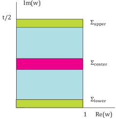
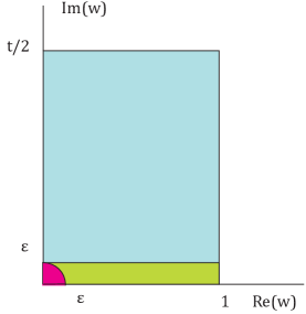
The $N=1$, $P=2$ configuration involves the following entropy integral,

$\displaystyle{\cal J}_{\varepsilon}(t,y)=\int_{\Sigma_{\varepsilon}}d^{2}w|{\cal N}(w)|^{2}h_{0}(w-y)h_{0}(w+y)$ (A.13)

where the ingredients are defined in (A.1) with ${\cal N}_{0}=-i$. The shifts by $\pm y$ cancel in the second term on the second line above upon taking the imaginary part in view of the fact that $\tau=it$ is purely imaginary. The integration region is defined as follows,

$\displaystyle\Sigma_{\varepsilon}$ $\displaystyle=$ $\displaystyle\left\{w=\alpha+i\beta{t\over 2}~{}\hbox{with}~{}~{}0\leq\alpha,\beta\leq 1~{}~{}\hbox{and}~{}~{}\varepsilon<|w|,~{}~{}\varepsilon<|1-w|\right\}$ (A.14)

with quarter disks of size $\varepsilon$ removed around the points $w=0,1$, as is represented in Figure 10. In the figure, we also represent the integration region $\Sigma_{\varepsilon}^{\prime}$, defined by

$\displaystyle\Sigma_{\varepsilon}^{\prime}$ $\displaystyle=$ $\displaystyle\left\{w=\alpha+i\beta{t\over 2}~{}~{}\hbox{with}~{}~{}0\leq\alpha\leq 1~{}~{}\hbox{and}~{}~{}\varepsilon_{0}<\beta<1\right\}$ (A.15)

which will be much easier to use in the actual calculations. Here, we set $t\varepsilon_{0}=2\varepsilon$.

Refer to caption
Figure 10: Regularizations $|w|>\varepsilon$ and ${\rm Im}(w)>\varepsilon$ inside the fundamental domain. The domain $\Sigma_{\varepsilon}$ consists of the union of the blue region and the green region (minus a corresponding quarter circle around the point $w=1$); the domain $\Sigma^{\prime}_{\varepsilon}$ consists only of the blue region.

A.2.1 Description of the expansion used

We shall obtain the asymptotic behavior as $t\to\infty$ with $\tau=it$. The integration region in $w$ will tends to $\infty$, and it is preferable to parametrize the integrand with a fixed range, as $\alpha,\beta$ do in (5.2). We need an expansion for large $\tau$ which is uniform throughout the integration region. Fortunately, for elliptic functions, this is easy to obtain using their product formula,

$\displaystyle\vartheta_{1}(w)=q_{0}\sin\pi w\prod_{n=1}^{\infty}\left(1-2q^{2n}\cos(2\pi w)+q^{4n}\right)$ (A.16)

with $q=e^{i\pi\tau}=e^{-\pi t}$, and $q_{0}$ an overall $t$-dependent factor which will cancel out of all our calculations. The behavior of the middle terms in the product, in terms of the fixed range parametrization of (5.2), are as follows,

$\displaystyle 2q^{2n}\cos(2\pi w)\sim e^{\pi i\tau(2n-\beta)-2\pi i\alpha}$ (A.17)

Since $0\leq\beta\leq 1$, all such terms are uniformly suppressed in $\Sigma_{\varepsilon}$, and will be omitted. Thus, we are left with the uniform approximation,

$\displaystyle\vartheta_{1}(w)\sim q_{0}\,\sin\pi w+{\cal O}(q)$ (A.18)

the higher order terms being suppressed by at least one power of $q$. The corresponding functions of (5.1) then take the form,

$\displaystyle{\cal N}(w)$ $\displaystyle=$ $\displaystyle-i\,{\sin\pi(w-y)\sin\pi(w+y)\over(\sin\pi w)^{2}}+{\cal O}(q)$
$\displaystyle h(w\pm y)$ $\displaystyle=$ $\displaystyle-{\pi i\over 2}\,{\sin\pi(w-\bar{w})\over|\sin\pi(w\pm y)|^{2}}-{2\pi\over t}{\rm Im}(w)+{\cal O}(q)$ (A.19)

Thus, the integral ${\cal J}_{\varepsilon}$ becomes,

$\displaystyle{\cal J}_{\varepsilon}(t,y)$ $\displaystyle=$ $\displaystyle{\pi^{2}\over 4}\int_{\Sigma_{\varepsilon}}{d^{2}w\over|\sin\pi w|^{4}}\left(i\sin\pi(w-\bar{w})+{4\over t}{\rm Im}(w)|\sin\pi(w+y)|^{2}\right)$
$\displaystyle\hskip 72.26999pt\times\left(i\sin\pi(w-\bar{w})+{4\over t}{\rm Im}(w)|\sin\pi(w-y)|^{2}\right)+{\cal O}(q)$

A.2.2 Changing regulator

It will turn out that the structure of the integrand, in terms of periodic functions, is not naturally regularized by the quarter disk cutoffs employed in the definition of $\Sigma_{\varepsilon}$. Instead, the domain $\Sigma_{\varepsilon}^{\prime}$ is more natural as the integration in $\alpha$ will then always have the same range. The difference involves the integral over the region in green in Figure 10, whose area tends to zero as $\varepsilon\to 0$, but whose contribution to ${\cal J}_{\varepsilon}$ does not. Thus, we shall decompose the regularized integral as follows,

$\displaystyle{\cal J}_{\varepsilon}(t,y)={\cal J}_{{\rm reg}}(t,y)+{\cal J}_{\varepsilon}^{(0)}(t,y)+{1\over t}{\cal J}_{\varepsilon}^{(1)}(t,y)+{1\over t^{2}}{\cal J}_{\varepsilon}^{(2)}(t,y)+{\cal O}(q)$ (A.21)

where we have the following expressions,

$\displaystyle{\cal J}_{\varepsilon}^{(0)}(t,y)$ $\displaystyle=$ $\displaystyle{\pi^{2}\over 4}\int_{\Sigma_{\varepsilon}^{\prime}}d^{2}w\,{|\sin\pi(w-\bar{w})|^{2}\over|\sin\pi w|^{4}}$
$\displaystyle{\cal J}_{\varepsilon}^{(1)}(t,y)$ $\displaystyle=$ $\displaystyle\pi^{2}\int_{\Sigma_{\varepsilon}^{\prime}}d^{2}w\,{i\sin\pi(w-\bar{w}){\rm Im}(w)\over|\sin\pi w|^{4}}|\sin\pi(w+y)|^{2}+(y\to-y)$
$\displaystyle{\cal J}_{\varepsilon}^{(2)}(t,y)$ $\displaystyle=$ $\displaystyle 4\pi^{2}\int_{\Sigma_{\varepsilon}^{\prime}}d^{2}w\,{{\rm Im}(w)^{2}\over|\sin\pi w|^{4}}|\sin\pi(w+y)|^{2}|\sin\pi(w-y)|^{2}$ (A.22)

and the term ${\cal J}_{{\rm reg}}$ accounting for the difference in regulators is given by,

$\displaystyle{\cal J}_{{\rm reg}}(t,y)$ $\displaystyle=$ $\displaystyle{\pi^{2}\over 4}\int_{\left(\Sigma_{\varepsilon}-\Sigma_{\varepsilon}^{\prime}\right)}{d^{2}w\over|\sin\pi w|^{4}}\left(i\sin\pi(w-\bar{w})+{4\over t}{\rm Im}(w)|\sin\pi(w+y)|^{2}\right)$
$\displaystyle\hskip 72.26999pt\times\left(i\sin\pi(w-\bar{w})+{4\over t}{\rm Im}(w)|\sin\pi(w-y)|^{2}\right)+{\cal O}(q)$

The $y$-dependence of these integrals is easily exposed: ${\cal J}_{\varepsilon}^{(0)}(t,y)$ is simply independent of $y$; while the other two integrals take on the following $y$-dependence:

$\displaystyle{\cal J}_{\varepsilon}^{(1)}(t,y)$ $\displaystyle=$ $\displaystyle 2\pi^{2}\cos^{2}\pi y\int_{\Sigma_{\varepsilon}^{\prime}}d^{2}w\,{i\sin\pi(w-\bar{w}){\rm Im}(w)\over|\sin\pi w|^{2}}$
$\displaystyle+2\pi^{2}\sin^{2}\pi y\int_{\Sigma_{\varepsilon}^{\prime}}d^{2}w\,{i\sin\pi(w-\bar{w}){\rm Im}(w)|\cos\pi w|^{2}\over|\sin\pi w|^{4}}$
$\displaystyle{\cal J}_{\varepsilon}^{(2)}(t,y)$ $\displaystyle=$ $\displaystyle 4\pi^{2}\cos^{4}\pi y\int_{\Sigma_{\varepsilon}^{\prime}}d^{2}w\,{\rm Im}(w)^{2}$ (A.24)
$\displaystyle+4\pi^{2}\sin^{4}\pi y\int_{\Sigma_{\varepsilon}^{\prime}}d^{2}w\,{{\rm Im}(w)^{2}|\cos\pi w|^{4}\over|\sin\pi w|^{4}}$
$\displaystyle-4\pi^{2}\sin^{2}\pi y\cos^{2}\pi y\int_{\Sigma_{\varepsilon}^{\prime}}d^{2}w\,{\rm Im}(w)^{2}\left({\cos^{2}\pi\bar{w}\over\sin^{2}\pi\bar{w}}+{\cos^{2}\pi w\over\sin^{2}\pi w}\right)$

A.2.3 Expansions

We will evaluate the above integrals by expanding the denominators in a uniformly convergent expansion (for $\varepsilon>0$), then carry out the integrals, and re-sum the results. We shall use the following expansions,

$\displaystyle{1\over\sin\pi w}$ $\displaystyle=$ $\displaystyle-2i\sum_{n=0}^{\infty}e^{i\pi w(2n+1)}$
$\displaystyle{1\over\sin^{2}\pi w}$ $\displaystyle=$ $\displaystyle-4\sum_{n=1}^{\infty}n\,e^{2\pi inw}$
$\displaystyle{\cos\pi w\over\sin^{2}\pi w}$ $\displaystyle=$ $\displaystyle-2\sum_{n=0}^{\infty}(2n+1)e^{i\pi w(2n+1)}$ (A.25)

We shall also use the following resummation formulas in the approximation where we neglect corrections suppressed by $e^{-\pi t}$, and contributions which vanish in the limit where $\varepsilon_{0}\to 0$,

$\displaystyle\sum_{n=1}^{\infty}{1\over n}e^{-2\pi tn\varepsilon_{0}}$ $\displaystyle\approx$ $\displaystyle-\ln(2\pi t\varepsilon_{0})$
$\displaystyle\sum_{n=1}^{\infty}e^{-2\pi tn\varepsilon_{0}}$ $\displaystyle\approx$ $\displaystyle{1\over 2\pi t\varepsilon_{0}}$
$\displaystyle\sum_{n=1}^{\infty}n\,e^{-2\pi tn\varepsilon_{0}}$ $\displaystyle\approx$ $\displaystyle{1\over 4\pi^{2}t^{2}\varepsilon_{0}^{2}}$ (A.26)

A.2.4 Evaluation of ${\cal J}_{\varepsilon}^{(0)}$

We begin by writing $w=\alpha+i\beta t/2$, and recast the integral in the following way,

$\displaystyle{\cal J}_{\varepsilon}^{(0)}(t,y)=2\pi^{2}t\int_{0}^{1}d\alpha\int_{\varepsilon_{0}}^{1}d\beta\,|\sin i\pi t\beta|^{2}\sum_{m,n=1}^{\infty}mn\,e^{2\pi i\alpha(m-n)-\pi t\beta(m+n)}$ (A.27)

The integral over $\alpha$ makes the resulting double sum collapse to a single sum,

$\displaystyle{\cal J}_{\varepsilon}^{(0)}(t,y)=2\pi^{2}t\sum_{n=1}^{\infty}n^{2}\int_{\varepsilon_{0}}^{1}d\beta\,|\sin i\pi t\beta|^{2}e^{-2\pi t\beta n}$ (A.28)

Expressing $\sin\pi(w-\bar{w})$ in terms of $e^{\pm\pi t\beta}$, we may rearrange the expansion as follows,

$\displaystyle{\cal J}_{\varepsilon}^{(0)}(t,y)={\pi^{2}t\over 2}+{\pi^{2}t\over 2}\sum_{n=1}^{\infty}\int_{\varepsilon_{0}}^{1}d\beta\,e^{-2\pi tn\beta}\,\left((n-1)^{2}+(n+1)^{2}-2n^{2}\right)$ (A.29)

The terms in parentheses simplify to give the value 2, and the remaining integral and sum are easily carried out, to find,

$\displaystyle{\cal J}_{\varepsilon}^{(0)}(t,y)={\pi^{2}t\over 2}+{\pi\over 2}\ln\left(1-e^{-2\pi t}\right)-{\pi\over 2}\ln\left(1-e^{-2\pi t\varepsilon_{0}}\right)$ (A.30)

To be consistent with the approximation we have made, we must drop the second term on the right, and approximate the formula for $\varepsilon\ll 1$, and we find,

$\displaystyle{\cal J}_{\varepsilon}^{(0)}(t,y)={\pi^{2}\over 2}t-{\pi\over 2}\ln\left(4\pi\varepsilon\right)$ (A.31)

A.2.5 Evaluation of ${\cal J}_{\varepsilon}^{(1)}$

The evaluation of ${\cal J}_{\varepsilon}^{(1)}$ involves two integrals,

$\displaystyle{\cal J}_{\varepsilon}^{(1)}=\pi^{2}{\cal K}_{1}\cos^{2}\pi y+\pi^{2}{\cal K}_{2}\sin^{2}\pi y$ (A.32)

where the integrals proper are given by,

$\displaystyle{\cal K}_{1}$ $\displaystyle=$ $\displaystyle 2\int_{\Sigma_{\varepsilon}^{\prime}}d^{2}w\,{i\,\sin\pi(w-\bar{w}){\rm Im}(w)\over|\sin\pi w|^{2}}$
$\displaystyle{\cal K}_{2}$ $\displaystyle=$ $\displaystyle 2\int_{\Sigma_{\varepsilon}^{\prime}}d^{2}w\,{i\,\sin\pi(w-\bar{w}){\rm Im}(w)|\cos\pi w|^{2}\over|\sin\pi w|^{4}}$ (A.33)

To compute ${\cal K}_{1}$, we make use of the first formula in (A.2.3), express $w$ in terms of $\alpha,\beta$, and carry out the integral over $\alpha$. The result is,

$\displaystyle{\cal K}_{1}=t^{2}\sum_{n=0}^{\infty}\int^{1}_{\varepsilon_{0}}d\beta\,\beta\left(e^{-2\pi t\beta(n+1)}-e^{-2\pi t\beta n}\right)$ (A.34)

all terms in the sum, except the second term for $n=0$, cancel one another pairwise, a so that we are left with,

$\displaystyle{\cal K}_{1}=-{1\over 2}t^{2}$ (A.35)

To compute ${\cal K}_{2}$, we make use of the fourth formula in (A.2.3), express $w$ in terms of $\alpha,\beta$, and carry out the integral over $\alpha$. The result is,

$\displaystyle{\cal K}_{2}=t^{2}\int^{1}_{\varepsilon_{0}}d\beta\,\beta\sum_{n=0}^{\infty}(2n+1)^{2}\,e^{-\pi t\beta(2n+1)}\left(e^{-\pi t\beta}-e^{\pi t\beta}\right)$ (A.36)

Combining the terms in the sum by shifting $n\to n-1$ in the first term, and then using $(2n-1)^{2}-(2n+1)^{2}=-8n$, gives the following simplified sum,

$\displaystyle{\cal K}_{2}=t^{2}\int^{1}_{\varepsilon_{0}}d\beta\left(-\beta-8\sum_{n=1}^{\infty}\beta n\,e^{-2\pi t\beta n}\right)$ (A.37)

Computing each individual integral, within the approximation of neglecting terms suppressed by $e^{-\pi t}$, we find,

$\displaystyle\int^{1}_{\varepsilon_{0}}d\beta\,\beta\,n\,e^{-2\pi t\beta n}\approx\left({\varepsilon_{0}\over 2\pi t}+{1\over 4\pi^{2}nt^{2}}\right)e^{-2\pi t\varepsilon_{0}}$ (A.38)

Carrying out the sum over $n$ gives,

$\displaystyle K_{2}=-{t^{2}\over 2}-{2\over\pi^{2}}+{2\over\pi^{2}}\ln(2\pi t\varepsilon_{0})$ (A.39)

Putting all together, we find,

$\displaystyle{\cal J}^{(1)}_{\varepsilon}(t,y)=-{\pi^{2}t^{2}\over 2}-2\sin^{2}\pi y+2\sin^{2}\pi y\,\ln(4\pi\varepsilon)$ (A.40)

A.2.6 Evaluation of ${\cal J}_{\varepsilon}^{(2)}$

The evaluation of ${\cal J}_{\varepsilon}^{(2)}$ involves 3 integrals,

$\displaystyle{\cal J}^{(2)}_{\varepsilon}=4\pi^{2}\cos^{4}\pi y\,{\cal K}_{3}-4\pi^{2}\sin^{2}\pi y\cos^{2}\pi y{\cal K}_{4}+4\pi^{2}\sin^{4}\pi y\,{\cal K}_{5}$ (A.41)

with

$\displaystyle{\cal K}_{3}$ $\displaystyle=$ $\displaystyle\int_{\Sigma_{\varepsilon}^{\prime}}d^{2}w\,{\rm Im}(w)^{2}$
$\displaystyle{\cal K}_{4}$ $\displaystyle=$ $\displaystyle\int_{\Sigma_{\varepsilon}^{\prime}}d^{2}w\,{\rm Im}(w)^{2}\left({\cos^{2}\pi w\over\sin^{2}\pi w}+{\cos^{2}\pi\bar{w}\over\sin^{2}\pi\bar{w}}\right)$
$\displaystyle{\cal K}_{5}$ $\displaystyle=$ $\displaystyle\int_{\Sigma_{\varepsilon}^{\prime}}d^{2}w\,{\rm Im}(w)^{2}\left|{\cos\pi w\over\sin\pi w}\right|^{4}$ (A.42)

The first integral is trivial to evaluate. For the second integral, we use the series expansion on the second line of (A.2.3), and its complex conjugate. Carrying out the $\alpha$-integration, it follows that only the $n=0$ in those expansions contributes, so that we get,

$\displaystyle{\cal K}_{3}$ $\displaystyle=$ $\displaystyle{t^{3}\over 24}$
$\displaystyle{\cal K}_{4}$ $\displaystyle=$ $\displaystyle-2{\cal K}_{3}=-{t^{3}\over 12}$ (A.43)

To calculate the integral ${\cal K}_{5}$ we use again the second line expansion in (A.2.3) to proceed,

$\displaystyle{\cal K}_{5}=\sum_{m,n=0}^{\infty}\left(\delta_{m,0}+4m\right)\left(\delta_{n,0}+4n\right)\int_{\Sigma_{\varepsilon}}d^{2}w{\rm Im}(w)^{2}\,e^{2\pi imw-2\pi in\bar{w}}$ (A.44)

Carrying out the $\alpha$-integral makes the double sum collapse to only $m=n$ contributions in terms on an integral over $\beta$,

$\displaystyle{\cal K}_{5}={t^{3}\over 24}+2t^{3}\sum_{n=1}^{\infty}\int^{1}_{\varepsilon_{0}}d\beta\,\beta^{2}n^{2}\,e^{-2\pi t\beta n}$ (A.45)

Neglecting again contributions suppressed by $e^{-\pi t}$, we find,

$\displaystyle\int^{1}_{\varepsilon_{0}}d\beta\,\beta^{2}n^{2}\,e^{-2\pi t\beta n}\approx\left({1\over 2\pi^{3}n}+{t\varepsilon_{0}\over\pi^{2}}+{t^{2}\varepsilon_{0}^{2}n\over\pi}\right)e^{-2\pi tn\varepsilon_{0}}$ (A.46)

Using the resummation formulas of (A.2.3), we can put all parts together gives,

$\displaystyle{\cal K}_{5}={t^{3}\over 24}+{3\over 4\pi^{3}}-{1\over 2\pi^{3}}\ln(2\pi t\varepsilon_{0})$ (A.47)

The total contribution to ${\cal J}_{\varepsilon}^{(2)}$ is then found to be,

$\displaystyle{\cal J}^{(2)}_{\varepsilon}={\pi^{2}t^{3}\over 6}+{3\over\pi}\sin^{4}\pi y-{2\over\pi}\sin^{4}\pi y\,\ln(4\pi\varepsilon)$ (A.48)

A.2.7 Evaluation of ${\cal J}_{{\rm reg}}$

The regions near $w=0$ and $w=1$ will give equal contributions, which may be approximated by the leading term of the integrand near $w=0$, since the divergence is only logarithmic. That contribution may be approximated by,

$\displaystyle{\cal J}_{{\rm reg}}=2\left(1-{2\over\pi t}\sin^{2}\pi y\right)^{2}{\cal I}\hskip 72.26999pt{\cal I}=\int_{\left(\Sigma_{\varepsilon}-\Sigma_{\varepsilon}^{\prime}\right)}{d^{2}w\over|w|^{4}}\,{\rm Im}(w)^{2}$ (A.49)

The factor of 2 accounts for the contributions from both $w=0$ and $w=1$. Expressing $w=\varepsilon(x+iy)$, the integral may be written as follows,

$\displaystyle{\cal I}=\int_{0}^{1/\varepsilon}dx\int_{0}^{1}dy{y^{2}\over(x^{2}+y^{2})^{2}}\theta(x^{2}+y^{2}-1)$ (A.50)

In the limit $\varepsilon\to 0$, we may let the upper integration limit tend to $\infty$. Changing variables to polar coordinates, $x=r\cos\psi,~{}y=r\sin\psi$, we obtain,

$\displaystyle{\cal I}=\int_{0}^{\pi/2}d\psi\int_{1}^{1/\sin\psi}dr\,{\sin^{2}\psi\over r}={\pi\over 4}\ln 2-{\pi\over 8}$ (A.51)

The last integral was obtained using MAPLE.

A.2.8 Assembling all contributions to ${\cal J}_{\varepsilon}$

Combining the contributions from ${\cal J}_{{\rm reg}},{\cal J}_{\varepsilon}^{(0)},{\cal J}_{\varepsilon}^{(1)},{\cal J}_{\varepsilon}^{(2)}$, we find,

$\displaystyle{\cal J}_{\varepsilon}(t,y)=-{\pi\over 2}\ln(2\pi\varepsilon)\left(1-{2\over\pi t}\sin^{2}\pi y\right)^{2}+{\pi^{2}\over 6}t-{\pi\over 4}-{1\over t}\sin^{2}\pi y+{2\over\pi t^{2}}\sin^{4}\pi y$ (A.52)

Next, we shall express this result with the help of the central charge of the bulk CFTs, which in turn is proportional to $Q_{A}Q^{A}$. We use the relation with the charges,

$\displaystyle Q\cdot Q=32\pi^{4}\left(|\vec{\ell}_{1}|\,|\vec{\ell}_{2}|-\vec{\ell}_{1}\cdot\vec{\ell}_{2}\right)\left(1-{2\over\pi t}\sin^{2}\pi y\right)^{2}$ (A.53)

Thus, we have

$\displaystyle S_{A}=-{Q\cdot Q\over 8\pi^{2}G_{N}}\ln(2\pi\varepsilon)+S_{{\rm\scriptstyle bcft}}$ (A.54)

where the finite boundary conformal field theory entanglement entropy part $g_{\rm bcft}$ is given by,

$\displaystyle S_{{\rm\scriptstyle bcft}}={4\pi^{2}\over G_{N}}\left(|\vec{\ell}_{1}|\,|\vec{\ell}_{2}|-\vec{\ell}_{1}\cdot\vec{\ell}_{2}\right)\left({\pi t\over 3}-{1\over 2}-{2\over\pi t}\sin^{2}\pi y+{4\over\pi^{2}t^{2}}\sin^{4}\pi y\right)$ (A.55)

The dominant term at large $t$ agrees with the funnel.

References

  • [1] J. M. Maldacena, โ€œThe Large N limit of superconformal field theories and supergravity,โ€ Adv. Theor. Math. Phys.  2 (1998) 231 [Int. J. Theor. Phys.  38 (1999) 1113] [hep-th/9711200].
  • [2] S. S. Gubser, I. R. Klebanov and A. M. Polyakov, โ€œGauge theory correlators from noncritical string theory,โ€ Phys. Lett. B 428 (1998) 105 [hep-th/9802109].
  • [3] E. Witten, โ€œAnti-de Sitter space and holography,โ€ Adv. Theor. Math. Phys.  2 (1998) 253 [hep-th/9802150].
  • [4] J. L. Cardy, โ€œBoundary Conditions, Fusion Rules and the Verlinde Formula,โ€ Nucl. Phys. B 324 (1989) 581.
  • [5] E. Dโ€™Hoker, J. Estes and M. Gutperle, โ€œInterface Yang-Mills, supersymmetry, and Janus,โ€ Nucl. Phys. B 753 (2006) 16 [hep-th/0603013].
  • [6] D. Gaiotto and E. Witten, โ€œSupersymmetric Boundary Conditions in N=4 Super Yang-Mills Theory,โ€ arXiv:0804.2902 [hep-th].
  • [7] A. Hanany and E. Witten, โ€œType IIB superstrings, BPS monopoles, and three-dimensional gauge dynamics,โ€ Nucl. Phys. B 492 (1997) 152 [hep-th/9611230].
  • [8] D. Gaiotto and E. Witten, โ€œJanus Configurations, Chern-Simons Couplings, And The theta-Angle in N=4 Super Yang-Mills Theory,โ€ JHEP 1006 (2010) 097 [arXiv:0804.2907 [hep-th]].
  • [9] D. Gaiotto and E. Witten, โ€œS-Duality of Boundary Conditions In N=4 Super Yang-Mills Theory,โ€ arXiv:0807.3720 [hep-th].
  • [10] B. Assel, C. Bachas, J. Estes and J. Gomis, โ€œHolographic Duals of D=3 N=4 Superconformal Field Theories,โ€ JHEP 1108 (2011) 087 [arXiv:1106.4253 [hep-th]].
  • [11] O. Aharony, L. Berdichevsky, M. Berkooz and I. Shamir, โ€œNear-horizon solutions for D3-branes ending on 5-branes,โ€ Phys. Rev. D 84 (2011) 126003 [arXiv:1106.1870 [hep-th]].
  • [12] R. Benichou and J. Estes, โ€œGeometry of Open Strings Ending on Backreacting D3-Branes,โ€ JHEP 1203 (2012) 025 [arXiv:1112.3035 [hep-th]].
  • [13] D. Bak, M. Gutperle and S. Hirano, โ€œA Dilatonic deformation of AdS(5) and its field theory dual,โ€ JHEP 0305 (2003) 072 [hep-th/0304129].
  • [14] E. Dโ€™Hoker, J. Estes and M. Gutperle, โ€œExact half-BPS Type IIB interface solutions. I. Local solution and supersymmetric Janus,โ€ JHEP 0706 (2007) 021 [arXiv:0705.0022 [hep-th]].
  • [15] E. Dโ€™Hoker, J. Estes and M. Gutperle, โ€œExact half-BPS Type IIB interface solutions. II. Flux solutions and multi-Janus,โ€ JHEP 0706 (2007) 022 [arXiv:0705.0024 [hep-th]].
  • [16] E. Dโ€™Hoker, J. Estes, M. Gutperle and D. Krym, โ€œExact Half-BPS Flux Solutions in M-theory. I: Local Solutions,โ€ JHEP 0808 (2008) 028 [arXiv:0806.0605 [hep-th]].
  • [17] E. Dโ€™Hoker, J. Estes, M. Gutperle and D. Krym, โ€œExact Half-BPS Flux Solutions in M-theory II: Global solutions asymptotic to AdS(7) x S**4,โ€ JHEP 0812 (2008) 044 [arXiv:0810.4647 [hep-th]].
  • [18] E. Dโ€™Hoker, J. Estes, M. Gutperle and D. Krym, โ€œExact Half-BPS Flux Solutions in M-theory III: Existence and rigidity of global solutions asymptotic to AdS(4) x S**7,โ€ JHEP 0909 (2009) 067 [arXiv:0906.0596 [hep-th]].
  • [19] A. Clark and A. Karch, โ€œSuper Janus,โ€ JHEP 0510, 094 (2005) [arXiv:hep-th/0506265].
  • [20] J. Gomis and C. Romelsberger, โ€œBubbling defect CFTโ€™s,โ€ JHEP 0608 (2006) 050 [arXiv:hep-th/0604155].
  • [21] O. Lunin, โ€œOn gravitational description of Wilson lines,โ€ JHEP 0606, 026 (2006) [arXiv:hep-th/0604133].
  • [22] O. Lunin, โ€œ1/2-BPS states in M theory and defects in the dual CFTs,โ€ JHEP 0710, 014 (2007) [arXiv:0704.3442 [hep-th]].
  • [23] S. Yamaguchi, โ€œBubbling geometries for half-BPS Wilson lines,โ€ Int. J. Mod. Phys.  A 22 (2007) 1353 [arXiv:hep-th/0601089].
  • [24] J. Gomis and F. Passerini, โ€œHolographic Wilson loops,โ€ JHEP 0608 (2006) 074 [arXiv:hep-th/0604007].
  • [25] J. Kumar and A. Rajaraman, โ€œNew supergravity solutions for branes in $AdS_{3}\times S^{3}$,โ€ Phys. Rev.  D 67 (2003) 125005 [arXiv:hep-th/0212145].
  • [26] J. Kumar and A. Rajaraman, โ€œSupergravity solutions for $AdS_{3}\times S^{3}$ branes,โ€ Phys. Rev.  D 69 (2004) 105023 [arXiv:hep-th/0310056].
  • [27] O. Lunin, โ€œBrane webs and 1/4-BPS geometries,โ€ JHEP 0809 (2008) 028 [arXiv:0802.0735 [hep-th]].
  • [28] E. Dโ€™Hoker, J. Estes, M. Gutperle, D. Krym and P. Sorba, โ€œHalf-BPS supergravity solutions and superalgebras,โ€ JHEP 0812, 047 (2008) [arXiv:0810.1484 [hep-th]].
  • [29] M. Chiodaroli, M. Gutperle and D. Krym, โ€œHalf-BPS Solutions locally asymptotic to $AdS_{3}\times S^{3}$ and interface conformal field theories,โ€ JHEP 1002 (2010) 066 [arXiv:0910.0466 [hep-th]].
  • [30] M. Chiodaroli, E. Dโ€™Hoker, M. Gutperle, โ€œOpen Worldsheets for Holographic Interfaces,โ€ JHEP 1003, 060 (2010). [arXiv:0912.4679 [hep-th]].
  • [31] M. Chiodaroli, E. Dโ€™Hoker, Y. Guo and M. Gutperle, โ€œExact half-BPS string-junction solutions in six-dimensional supergravity,โ€ JHEP 1112 (2011) 086 [arXiv:1107.1722 [hep-th]].
  • [32] L. J. Romans, โ€œSelfduality For Interacting Fields: Covariant Field Equations For Six-dimensional Chiral Supergravities,โ€ Nucl. Phys. B 276 (1986) 71.
  • [33] J. H. Schwarz, โ€œLectures on superstring and M theory dualities: Given at ICTP Spring School and at TASI Summer School,โ€ Nucl. Phys. Proc. Suppl.  55B (1997) 1 [hep-th/9607201].
  • [34] K. Dasgupta and S. Mukhi, โ€œBPS nature of three string junctions,โ€ Phys. Lett. B 423 (1998) 261 [hep-th/9711094].
  • [35] A. Sen, โ€œString network,โ€ JHEP 9803 (1998) 005 [hep-th/9711130].
  • [36] M. Chiodaroli, M. Gutperle, L. -Y. Hung, D. Krym, โ€œString Junctions and Holographic Interfaces,โ€ Phys. Rev.  D83, 026003 (2011). [arXiv:1010.2758 [hep-th]].
  • [37] C. G. Callan and J. M. Maldacena, โ€œBrane death and dynamics from the Born-Infeld action,โ€ Nucl. Phys. B 513 (1998) 198 [hep-th/9708147].
  • [38] A. Karch and L. Randall, โ€œOpen and closed string interpretation of SUSY CFTโ€™s on branes with boundaries,โ€ JHEP 0106 (2001) 063 [hep-th/0105132].
  • [39] T. Takayanagi, โ€œHolographic Dual of BCFT,โ€ Phys. Rev. Lett.  107 (2011) 101602 [arXiv:1105.5165 [hep-th]].
  • [40] M. Fujita, T. Takayanagi and E. Tonni, โ€œAspects of AdS/BCFT,โ€ JHEP 1111 (2011) 043 [arXiv:1108.5152 [hep-th]].
  • [41] M. Nozaki, T. Takayanagi and T. Ugajin, โ€œCentral Charges for BCFTs and Holography,โ€ arXiv:1205.1573 [hep-th].
  • [42] Y. Kwon, S. Nam, J. -D. Park and S. -H. Yi, โ€œAdS/BCFT Correspondence for Higher Curvature Gravity: An Example,โ€ arXiv:1201.1988 [hep-th].
  • [43] M. R. Setare and V. Kamali, โ€œTwo point functions of BCFT,โ€ arXiv:1109.3849 [hep-th].
  • [44] M. Alishahiha and R. Fareghbal, โ€œBoundary CFT from Holography,โ€ Phys. Rev. D 84, 106002 (2011) [arXiv:1108.5607 [hep-th]].
  • [45] M. Chiodaroli, E. Dโ€™Hoker and M. Gutperle, โ€œSimple holographic duals to boundary CFTs,โ€ arXiv:1111.6912 [hep-th].
  • [46] C. Bachas and M. Petropoulos, โ€œAnti-de Sitter D-branes,โ€ JHEP 0102 (2001) 025 [hep-th/0012234].
  • [47] J. Raeymaekers, K. P. Yogendran, โ€œSupersymmetric D-branes in the D1-D5 background,โ€ JHEP 0612 (2006) 022. [hep-th/0607150].
  • [48] E. Dโ€™Hoker and D. H. Phong, โ€œThe Geometry of String Perturbation Theory,โ€ Rev. Mod. Phys.  60, 917 (1988).
  • [49] I. Affleck and A. W. W. Ludwig, โ€œUniversal noninteger โ€™ground state degeneracyโ€™ in critical quantum systems,โ€ Phys. Rev. Lett.  67 (1991) 161.
  • [50] P. Calabrese and J. L. Cardy, โ€œEntanglement entropy and quantum field theory,โ€ J. Stat. Mech.  0406 (2004) P06002 [hep-th/0405152].
  • [51] S. Ryu and T. Takayanagi, โ€œHolographic derivation of entanglement entropy from AdS/CFT,โ€ Phys. Rev. Lett.  96 (2006) 181602 [hep-th/0603001].
  • [52] S. Ryu and T. Takayanagi, โ€œAspects of Holographic Entanglement Entropy,โ€ JHEP 0608 (2006) 045 [hep-th/0605073].
  • [53] M. Chiodaroli, M. Gutperle and L. Y. Hung, โ€œBoundary entropy of supersymmetric Janus solutions,โ€ JHEP 1009, 082 (2010) [arXiv:1005.4433 [hep-th]].
  • [54] John D. Fay, Theta Functions on Riemann Surfaces, Lecture Notes in Mathematics, Volume 352, Springer-Verlag 1973.
  • [55] O. Aharony, A. Hanany and B. Kol, โ€œWebs of (p,q) five-branes, five-dimensional field theories and grid diagrams,โ€ JHEP 9801 (1998) 002 [hep-th/9710116].
  • [56] O. Bergman and B. Kol, โ€œString webs and 1/4 BPS monopoles,โ€ Nucl. Phys. B 536 (1998) 149 [hep-th/9804160].