A simple formula for the series of constellations and quasi-constellations with boundaries

Abstract.

We obtain a very simple formula for the generating function of bipartite (resp. quasi-bipartite) planar maps with boundaries (holes) of prescribed lengths, which generalizes certain expressions obtained by Eynard in a book to appear. The formula is derived from a bijection due to Bouttier, Di Francesco and Guitter combined with a process (reminiscent of a construction of Pitman) of aggregating connected components of a forest into a single tree. The formula naturally extends to $p$-constellations and quasi-$p$-constellations with boundaries (the case $p=2$ corresponding to bipartite maps).

1. Introduction

Planar maps, i.e., connected graphs embedded on the sphere, have attracted a lot of attention since the seminal work of Tutte [21, 22]. By considering rooted maps (i.e., maps where a corner is marked ) and using a recursive approach, Tutte found beautiful counting formulas for many families of maps (bipartite, triangulations,…). Several features occur recurrently (see [3] for a unified treatment): the generating function $y=y(x)$ is typically algebraic, often lagrangean (i.e., there is a parametrization as $\{y=Q_{1}(t),x=Q_{2}(t)\}$, where $Q_{1}(.)$ and $Q_{2}(.)$ are explicit rational expressions), yielding simple (binomial-like) formulas for the counting coefficients $c_{n}$, and the asymptotics of the coefficients is in $c\ \!\gamma^{n}n^{-5/2}$ for some constants $c>0$ and $\gamma>1$. In this article we firstly focus on bipartite maps (all faces have even degree) and on quasi-bipartite maps (all faces have even degree except for two, which have odd degree). One of the first counting results obtained by Tutte is a strikingly simple formula (called formula of slicings) for the number $A[\ell_{1},\ldots,\ell_{r}]$ of maps with $r$ numbered faces $f_{1},\ldots,f_{r}$ of respective degrees $\ell_{1},\ldots,\ell_{r}$, each face having a marked corner (for simple parity reasons the number of odd $\ell_{i}$ must be even).

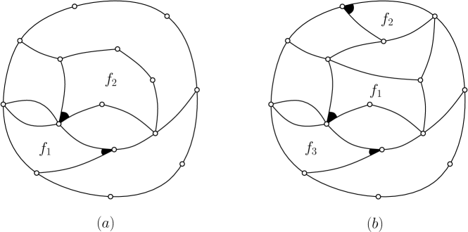
Figure 1. (a) A bipartite map with $2$ boundaries $f_{1},f_{2}$ of respective degree $4,6$. (b) A quasi-bipartite map with $3$ boundaries $f_{1},f_{2},f_{3}$ of respective degree $5,3,4$.

Solving a technically involved recurrence satisfied by these coefficients, he proved in [21] that when none or only two of the $\ell_{i}$ are odd (bipartite and quasi-bipartite case, respectively), then:

(1) $$A[\ell_{1},\ldots,\ell_{r}]=\frac{(e-1)!}{v!}\prod_{i=1}^{r}\alpha(\ell_{i}),\ \ \mathrm{with}\ \alpha(\ell):=\frac{\ell!}{\lfloor\ell/2\rfloor!\lfloor(\ell-1)/2\rfloor!},$$

where $e=\sum_{i=1}^{r}\ell_{i}/2$ and $v=e-r+2$ are the numbers of edges and vertices in such maps. The formula was recovered by Cori [11, 12] (using a certain encoding procedure for planar maps); and the formula in the bipartite case was rediscovered bijectively by Schaeffer [19], based on a correspondence with so-called blossoming trees. Alternatively one can use a more recent bijection by Bouttier, Di Francesco and Guitter [7] (based on a correspondence with so-called mobiles) which itself extends earlier constructions by Cori and Vauquelin [13] and by Schaeffer [18, Sec. 6.1] for quadrangulations. The bijection with mobiles yields the following: if we denote by $R\equiv R(t)\equiv R(t;x_{1},x_{2},\ldots)$ the generating function specified by

(2) $$R=t+\sum_{i\geq 1}x_{i}\binom{2i-1}{i}R^{i}.$$

and denote by $M(t)\equiv M(t;x_{1},x_{2},\ldots)$ the generating function of rooted bipartite maps, where $t$ marks the number of vertices and $x_{i}$ marks the number of faces of degree $2i$ for $i\geq 1$, then $M^{\prime}(t)=2R(t)$. And one easily recovers (1) in the bipartite case by an application of the Lagrange inversion formula to extract the coefficients of $R(t)$.

As we can see, maps might satisfy beautiful counting formulas, regarding counting coefficients . Regarding generating functions, formulas can be very nice and compact as well. In a book to be published [14], Eynard gives an iterative procedure (based on residue calculations) to compute the generating function of maps of arbitrary genus and with several marked faces, which we will call boundary-faces (or shortly boundaries). In certain cases, this yields an explicit expression for the generating function. For example, he obtains formulas for the (multivariate) generating functions of bipartite and quasi-bipartite maps with two or three boundaries of arbitrary lengths $\ell_{1},\ell_{2},\ell_{3}$ (in the quasi-bipartite case two of these lengths are odd), where $t$ marks the number of vertices and $x_{i}$ marks the number of non-boundary faces of degree $2i$:

(3) $$G_{\ell_{1},\ell_{2}} = \gamma^{\ell_{1}+\ell_{2}}\sum_{j=0}^{\left\lfloor\ell_{2}/2\right\rfloor}(\ell_{2}-2j)\frac{\ell_{1}!\ell_{2}!}{j!(\frac{\ell_{1}-\ell_{2}}{2}+j)!(\frac{\ell_{1}+\ell_{2}}{2}-j)!(\ell_{2}-j)!},$$

(4) $$G_{\ell_{1},\ell_{2},\ell_{3}} = \frac{\gamma^{\ell_{1}+\ell_{2}+\ell_{3}-1}}{y^{\prime}(1)}\left(\prod_{i=1}^{3}\frac{\ell_{i}!}{\left\lfloor\ell_{i}/2\right\rfloor!\left\lfloor(\ell_{i}-1)/2\right\rfloor!}\right).$$

In these formulas the series $\gamma$ and $y^{\prime}(1)$ are closely related to $R(t)$, precisely $\gamma^{2}=R(t)$ and one can check that $y^{\prime}(1)=\gamma/R^{\prime}(t)$.

In the first part of this article, we obtain new formulas which generalize Eynard’s ones to any number of boundaries, both in the bipartite and the quasi-bipartite case. For $r\geq 1$ and $\ell_{1},\ldots,\ell_{r}$ positive integers, an even map of type $(\ell_{1},\ldots,\ell_{r})$ is a map with $r$ (numbered) marked faces —called boundary-faces— $f_{1},\ldots,f_{r}$ of degrees $\ell_{1},\ldots,\ell_{r}$, each boundary-face having a marked corner, and with all the other faces of even degree. (Note that there is an even number of odd $\ell_{i}$ by a simple parity argument.) Let $G_{\ell_{1},\ldots,\ell_{r}}:=G_{\ell_{1},\ldots,\ell_{r}}(t;x_{1},x_{2},\ldots)$ be the corresponding generating function where $t$ marks the number of vertices and $x_{i}$ marks the number of non-boundary faces of degree $2i$. Our main result is:

Theorem 1.

When none or only two of the $\ell_{i}$ are odd, then the following formula holds:

(5) $$G_{\ell_{1},\ldots,\ell_{r}}=\Big{(}\prod_{i=1}^{r}\alpha(\ell_{i})\Big{)}\cdot\frac{1}{s}\cdot\frac{\mathrm{d}^{r-\!2}}{\mathrm{d}t^{r-\!2}}R^{s},$$

$$\textrm{with}\ \alpha(\ell)=\frac{\ell!}{\lfloor\tfrac{\ell}{2}\rfloor!\lfloor\tfrac{\ell-1}{2}\rfloor!},\ s=\frac{\ell_{1}+\cdots+\ell_{r}}{2},\textrm{ where }R\textrm{ is given by~{}\eqref{eq:seriesR}}.$$

Our formula covers all parity cases for the $\ell_{i}$ when $r\leq 3$. For $r=1$, the formula reads $G_{2a}\ \!\!^{\prime}=\binom{2a}{a}R^{a}$, which is a direct consequence of the bijection with mobiles. For $r=2$ the formula reads $G_{\ell_{1},\ell_{2}}=\alpha(\ell_{1})\alpha(\ell_{2})R^{s}/s$ (which simplifies the constant in (3)). And for $r=3$ the formula reads $G_{\ell_{1},\ell_{2},\ell_{3}}=\alpha(\ell_{1})\alpha(\ell_{2})\alpha(\ell_{3})R^{\prime}R^{s-1}$. Note that (5) also “contains” the formula of slicings (1), by noticing that $A[\ell_{1},\ldots,\ell_{r}]$ equals the evaluation of $G_{\ell_{1},\ldots,\ell_{r}}$ at $\{t=1;x_{1}=0,x_{2}=0,\ldots\}$, which equals $(\prod_{i=1}^{r}\alpha(\ell_{i}))\cdot\frac{(s-1)!}{(s-r+2)!}$. Hence, (5) can be seen as an “interpolation” between the two formulas of Eynard given above and Tutte’s formula of slicings. In addition, (5) has the nice feature that the expression of $G_{\ell_{1},\ldots,\ell_{r}}$ splits into two factors: (i) a constant factor which itself is a product of independent contributions from every boundary, (ii) a series-factor that just depends on the number of boundaries and the total length of the boundaries.

Even though the coefficients of $G_{\ell_{1},\ldots,\ell_{r}}$ have simple binomial-like expressions (easy to obtain from (1)), it does not explain why at the level of generating functions the expression (5) is so simple (and it would not be obvious to guess  (5) by just looking at (1)). Relying on the bijection with mobiles (recalled in Section 2), we give a transparent proof of (5). In the bipartite case, our construction (described in Section 3) starts from a forest of mobiles with some marked vertices, and then we aggregate the connected components so as to obtain a single mobile with some marked black vertices of fixed degrees (these black vertices correspond to the boundary-faces). The idea of aggregating connected components as we do is reminiscent of a construction due to Pitman [17], giving for instance a very simple proof (see [1, Chap. 26]) that the number of Cayley trees with $n$ nodes is $n^{n-2}$. Then we show in Section 4 that the formula in the quasi-bipartite case can be obtained by a reduction to the bipartite case  This reduction is done bijectively with the help of auxiliary trees called blossoming trees. Let us mention that these blossoming trees have been introduced in another bijection with bipartite maps [19]. We could alternatively use this bijection to prove Theorem 1 in the bipartite case (none of the $\ell_{i}$ is odd). But in order to encode quasi-bipartite maps, one would have to use extensions of this bijection [5, 6] in which the encoding would become rather involved. This is the reason why we rely on bijections with mobiles, as given in [7].

In the second part of the article, we extend the formula of Theorem 1 to constellations and quasi-constellations, families of maps which naturally generalize bipartite and quasi-bipartite maps. Define an hypermap as an eulerian map (map with all faces of even degree) whose faces are bicolored —there are dark faces and light faces— such that any edge has a dark face on one side and a light face on the other side . Define a $p$-hypermap as a hypermap whose dark faces are of degree $p$ (note that classical maps correspond to $2$-hypermaps, since each edge can be blown into a dark face of degree $2$). Note that the degrees of light faces in a $p$-hypermap add up to a multiple of $p$. A $p$-constellation is a $p$-hypermap such that the degrees of light faces are multiples of $p$, and a quasi $p$-constellation is a $p$-hypermap such that exactly two light faces have a degree not multiple of $p$. By the identification with maps, $2$-constellations and quasi $2$-constellations correspond respectively to bipartite maps and quasi-bipartite maps.

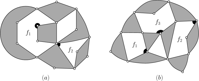
Figure 2. (a) A $4$-constellation with $2$ boundaries $f_{1},f_{2}$ of respective degree $8,4$. (b) A quasi-$3$-constellation with $3$ boundaries $f_{1},f_{2},f_{3}$ of respective degree $4,5,6$.

Bouttier, Di Francesco and Guitter [7] also described a bijection for hypermaps, in correspondence with more involved mobiles (recalled in Section 5.1). When applied to $p$-constellations, this bijection yields the following: if we denote by $R_{p}=R_{p}(t)=R_{p}(t;x_{1},x_{2},\ldots)$ the generating function specified by

(6) $$R_{p}=t+\sum_{i\geq 1}x_{i}\binom{pi-1}{i}R_{p}^{(p-1)i}.$$

and by $C_{p}(t)=C_{p}(t;x_{1},x_{2},\ldots)$ the generating function of rooted $p$-constellations (i.e., $p$-constellations with a marked corner incident to a light face) where $t$ marks the number of vertices and $x_{i}$ marks the number of light faces of degree $pi$ for $i\geq 1$, then the bijection of [7] ensures that $C_{p}^{\prime}(t)=\frac{p}{p-1}R_{p}(t)$.

We use this bijection and tools from Sections 3 and 4 to obtain the following formula for the generating function of constellations (proved in Section 5.2) and quasi-constellations (proved in Section 5.3). Let $G^{(p)}_{\ell_{1},\ldots,\ell_{r}}:=G^{(p)}_{\ell_{1},\ldots,\ell_{r}}(t;x_{1},x_{2},\ldots)$ be the generating function of $p$-hypermaps with $r$ (numbered) boundaries $f_{1},\ldots,f_{r}$ of degrees $\ell_{1},\ldots,\ell_{r}$, whose non-marked faces have degrees a multiple of $p$, where $t$ marks the number of vertices and $x_{i}$ marks the number of non-boundary faces of degree $pi$. Then:

Theorem 2.

When none or only two of the $\ell_{i}$ are not multiple of $p$, then the following formula holds:

(7) $$G^{(p)}_{\ell_{1},\ldots,\ell_{r}}=\Big{(}\prod_{i=1}^{r}\alpha(\ell_{i})\Big{)}\cdot\frac{c}{s}\cdot\frac{\mathrm{d}^{r-\!2}}{\mathrm{d}t^{r-\!2}}R_{p}^{s},\$$

$\textrm{where}\ \displaystyle{\alpha(\ell)=\frac{\ell!}{\lfloor\ell/p\rfloor!\left(\ell-\lfloor\ell/p\rfloor-1\right)!}},\ s=\frac{p-1}{p}(\ell_{1}+\cdots+\ell_{r}),\ R_{p}\textrm{ is given by~{}\eqref{eq:seriesRp}},$
and $c=\left\{\begin{array}[]{l}1,\textrm{~{}when every }\ell_{i}\textrm{~{}is a multiple of }p,\\ p-1,\textrm{~{}when exactly two }\ell_{i}\textrm{~{}are not multiple of }p.\end{array}\right.$

First note that Theorem 1 is the direct application of Theorem 2 when $p=2$. Moreover, this yields the following extension of Tutte’s slicing formula:

Corollary 3.

For $p\geq 2$, let $A^{(p)}[\ell_{1},\ldots,\ell_{r}]$ be the number of $p$-hypermaps with exactly $r$ numbered light faces $f_{1},\ldots,f_{r}$ of respective degrees $\ell_{1},\ldots,\ell_{r}$, each light face having a marked corner.
When none or only two of the $\ell_{i}$ are not multiple of $p$ ($p$-constellations and quasi-$p$-constellations, respectively), then:

(8) $$A^{(p)}[\ell_{1},\ldots,\ell_{r}]=c\frac{(\epsilon-d-1)!}{v!}\prod_{i=1}^{r}\alpha(\ell_{i}),\ \ \mathrm{with}\ \alpha(\ell):=\frac{\ell!}{\lfloor\ell/p\rfloor!(\ell-\lfloor\ell/p\rfloor-1)!},$$

where $\epsilon=\sum_{i=1}^{r}\ell_{i}$ is the number of edges, $\displaystyle{d=\frac{\sum_{i=1}^{r}\ell_{i}}{p}}$ is the number of dark faces, and $v=\epsilon-d-r+2$ is the number of vertices,
and $c=\left\{\begin{array}[]{l}1,\textrm{~{}when every }\ell_{i}\textrm{~{}is a multiple of }p,\\ p-1,\textrm{~{}when exactly two }\ell_{i}\textrm{~{}are not multiple of }p.\end{array}\right.$

One gets (8) out of (7) by taking the evaluation of $G^{(p)}_{\ell_{1},\dots,\ell_{r}}$ at $\{t=1;x_{1}=0,x_{2}=0,\ldots\}$. The expression of the numbers $A^{(p)}[\ell_{1},\ldots,\ell_{r}]$ when all $\ell_{i}$ are multiples of $p$ has been discovered by Bousquet-Mélou and Schaeffer [4], but to our knowledge, the expression for quasi-constellations has not been given before (though it could also be obtained from Chapuy’s results [9], see the paragraphs after Lemma 10 and Lemma 22).

Note. This is the full version of a conference paper [10] entitled “A simple formula for the series of bipartite and quasi-bipartite maps with boundaries” presented at the conference FPSAC’12. In particular we extend here the formulas obtained in [10] to constellations and quasi-constellations. We would like to mention that very recently Bouttier and Guitter [8] have found extensions of the formulas from [10] in another direction, to so-called $2b$-irreducible bipartite maps (maps with all faces of degrees at least $2b$ and where all non-facial cycles have length at least $2b+2$).

Notation. We will often use the following notation: for $\mathcal{A}$ and $\mathcal{B}$ two (typically infinite) combinatorial classes and $a$ and $b$ two integers, write $a\cdot\mathcal{A}\simeq b\cdot\mathcal{B}$ if there is a “natural” $a$-to-$b$ correspondence between $\mathcal{A}$ and $\mathcal{B}$ (the correspondence will be explicit each time the notation is used) that preserves several parameters (which will be listed when the notation is used, typically the correspondence will preserve the face-degree distribution).

2. Bijection between vertex-pointed maps and mobiles

We recall here a well-known bijection due to Bouttier, Di Francesco and Guitter [7] between vertex-pointed planar maps and a certain family of decorated trees called mobiles. We actually follow a slight reformulation of the bijection given in [2]. A mobile is a plane tree (i.e., a planar map with one face) with vertices either black or white, with dangling half-edges —called buds— at black vertices, such that there is no white-white edge, and such that each black vertex has as many buds as white neighbours.The degree of a black vertex $v$ is the total number of incident half-edges (including the buds) incident to $v$. Starting from a planar map $G$ with a pointed vertex $v_{0}$, and where the vertices of $G$ are considered as white, one obtains a mobile $M$ as follows (see Figure 3):

• Endow $G$ with its geodesic orientation from $v_{0}$ (i.e., an edge $\{v,v^{\prime}\}$ is oriented from $v$ to $v^{\prime}$ if $v^{\prime}$ is one unit further than $v$ from $v_{0}$, and is left unoriented if $v$ and $v^{\prime}$ are at the same distance from $v_{0}$).

• Put a new black vertex in each face of $G$.

• Apply the following local rules to each edge (one rule for oriented edges and one rule for unoriented edges) of $G$:

  

• Delete the edges of $G$ and the vertex $v_{0}$.

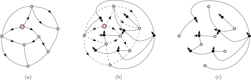
Figure 3. (a) A vertex-pointed map endowed with the geodesic orientation (with respect to the marked vertex). (b) The local rule is applied to each edge of the map. (c) The resulting mobile.

Theorem 4 (Bouttier, Di Francesco and Guitter [7]).

The above construction is a bijection between vertex-pointed maps and mobiles. Each non-root vertex in the map corresponds to a white vertex in the mobile. Each face of degree $i$ in the map corresponds to a black vertex of degree $i$ in the mobile.

A mobile is called bipartite when all black vertices have even degree, and is called quasi-bipartite when all black vertices have even degree except for two which have odd degree. Note that bipartite (resp. quasi-bipartite) mobiles correspond to bipartite (resp. quasi-bipartite) vertex-pointed maps.

Claim 5.

A mobile is bipartite iff it has no black-black edge. A mobile is quasi-bipartite iff the set of black-black edges forms a non-empty path whose extremities are the two black vertices of odd degrees.

Proof.

Let $T$ be a mobile and $F$ the forest formed by the black vertices and black-black edges of $T$. Note that for each black vertex of $T$, the degree and the number of incident black-black edges have same parity. Hence if $T$ is bipartite, $F$ has only vertices of even degree, so $F$ is empty; while if $T$ is quasi-bipartite, $F$ has two vertices of odd degree, so the only possibility is that the edges of $F$ form a non-empty path. ∎

A bipartite mobile is called rooted if it has a marked corner at a white vertex. Let $R:=R(t;x_{1},x_{2},\ldots)$ be the generating function of rooted bipartite mobiles, where $t$ marks the number of white vertices and $x_{i}$ marks the number of black vertices of degree $2i$ for $i\geq 1$. As shown in [7], a decomposition at the root ensures that $R$ is given by Equation (2); indeed if we denote by $S$ the generating function of bipartite mobiles rooted at a white leaf, then $R=t+RS$ and $S=\sum_{i\geq 1}x_{i}\binom{2i-1}{i}R^{i-1}$.

For a mobile $\gamma$ with marked black vertices $b_{1},\ldots,b_{r}$ of degrees $2a_{1},\ldots,2a_{r}$, the associated pruned mobile $\widehat{\gamma}$ obtained from $\gamma$ by deleting the buds at the marked vertices (thus the marked vertices get degrees $a_{1},\ldots,a_{r}$). Conversely, such a pruned mobile yields $\prod_{i=1}^{r}{2a_{i}-1\choose a_{i}}$ mobiles (because of the number of ways to place the buds around the marked black vertices). Hence, if we denote by $\mathcal{B}_{2a_{1},\dots,2a_{r}}$ the family of bipartite mobiles with $r$ marked black vertices of respective degree $2a_{1},\dots,2a_{r}$, and denote by $\widehat{\mathcal{B}}_{2a_{1},\dots,2a_{r}}$ the family of pruned bipartite mobiles with $r$ marked black vertices of respective degree $a_{1},\dots,a_{r}$, we have:

$$\mathcal{B}_{2a_{1},\dots,2a_{r}}\simeq\prod_{i=1}^{r}{2a_{i}-1\choose a_{i}}\widehat{\mathcal{B}}_{2a_{1},\dots,2a_{r}}.$$

3. Bipartite case

In this section, we consider the two following families:

• $\widehat{\mathcal{M}}_{2a_{1},\dots,2a_{r}}$ is the family of pruned bipartite mobiles with $r$ marked black vertices of respective degrees $a_{1},\dots,a_{r}$, the mobile being rooted at a corner of one of the marked vertices,

• $\mathcal{F}_{s}$ is the family of forests made of $s:=\sum_{i=1}^{r}a_{i}$ rooted bipartite mobiles, and where additionnally $r-1$ white vertices $w_{1},\ldots,w_{r-1}$ are marked.

Proposition 6.

There is an $(r-1)!$-to-$(r-1)!$ correspondence between the family $\widehat{\mathcal{M}}_{2a_{1},\dots,2a_{r}}$ and the family $\mathcal{F}_{s}$. If $\gamma\in\widehat{\mathcal{M}}_{2a_{1},\dots,2a_{r}}$ corresponds to $\gamma^{\prime}\in\mathcal{F}_{s}$, then each white vertex in $\gamma$ corresponds to a white vertex in $\gamma^{\prime}$, and each unmarked black vertex of degree $2i$ in $\gamma$ corresponds to a black vertex of degree $2i$ in $\gamma^{\prime}$.

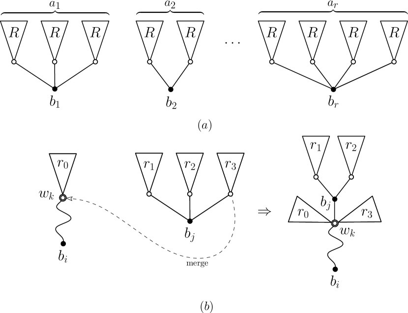
Figure 4. $(a)$ From a forest with $s=\sum_{i=1}^{r}{a_{i}}$ mobiles to $r$ components rooted at black vertices $b_{1},\dots,b_{r}$. $(b)$ Merging the component rooted at $b_{j}$ with the distinct component rooted at $b_{i}$ containing the marked white vertex $w_{k}$.

Proof.

We will describe the correspondence in both ways (see Figure 4). First, one can go from the forest to the pruned mobile through the following operations:

1. Group the first $a_{1}$ mobiles and bind them to a new black vertex $b_{1}$, then bind the next $a_{2}$ mobiles to a new black vertex $b_{2}$, and so on, to get a forest with $r$ connected components rooted at $b_{1},\dots,b_{r}$, see Figure 4(a).

2. The $r-1$ marked white vertices $w_{1},\dots,w_{r-1}$ are ordered, pick one of the $r-1$ components which do not contain $w_{r-1}$. Bind this component to $w_{r-1}$ by merging $w_{r-1}$ with the rightmost white neighbour of $b_{i}$, see Figure 4(b). Repeat the operation for each $w_{r-i}$ to reduce the number of components to one ($r-i$ possibilities in the choice of the connected component at the $i$th step), thus getting a decorated bipartite tree rooted at a corner incident to some $b_{j}$, and having $r$ black vertices $b_{1},\dots,b_{r}$ without buds.

Conversely, one can go from the pruned mobile to the forest through the following operations:

1. Pick one marked black vertex $b_{k}$, but the root, and separate it as in Figure 4(b) read from right to left. This creates a new connected component, rooted at $b_{k}$.

2. Repeat this operation, choosing at each step ($r-i$ possibilites at the $i$th step) a marked black vertex that is not the root in its connected component, until one gets $r$ connected components, each being rooted at one of the marked black vertices $\{b_{1},\ldots,b_{r}\}$ of respective degrees $a_{1},\ldots,a_{r}$.

3. Remove all marked black vertices $b_{1},\ldots,b_{r}$ and their incident edges; this yields a forest of $s$ rooted bipartite mobiles.

In both ways, there are $\prod_{i=1}^{r-1}(r-i)=(r-1)!$ possibilities, that is, the correspondence is $(r-1)!$-to-$(r-1)!$. ∎

As a corollary we obtain the formula of Theorem 1 in the bipartite case:

Corollary 7.

For $r\geq 1$ and $a_{1},\ldots,a_{r}$ positive integers, the generating function $G_{2a_{1},\ldots,2a_{r}}$ satisfies (5), i.e.,

(9) $$G_{2a_{1},\dots,2a_{r}}=\left(\prod_{i=1}^{r}\frac{(2a_{i})!}{a_{i}!(a_{i}-1)!}\right)\cdot\frac{1}{s}\cdot\frac{\mathrm{d}^{r-\!2}}{\mathrm{d}t^{r-\!2}}R^{s},\ \ \mathrm{where}\ s=\sum_{i=1}^{r}a_{i}.$$

Proof.

As mentioned in the introduction, for $r=1$ the expression reads $G_{2a}\ \!\!^{\prime}=\binom{2a}{a}R^{a}$, which is a direct consequence of the bijection with mobiles (indeed $G_{2a}\ \!\!^{\prime}$ is the series of mobiles with a marked black vertex $v$ of degree $2a$, with a marked corner incident to $v$). So we now assume $r\geq 2$. Let $B_{2a_{1},\dots,2a_{r}}=B_{2a_{1},\dots,2a_{r}}(t;x_{1},x_{2},\ldots)$ be the generating function of $\mathcal{B}_{2a_{1},\dots,2a_{r}}$, where $t$ marks the number of white vertices and $x_{i}$ marks the number of black vertices of degree $2i$. Let $\widehat{M}_{2a_{1},\dots,2a_{r}}=\widehat{M}_{2a_{1},\dots,2a_{r}}(t;x_{1},x_{2},\ldots)$ be the generating function of $\widehat{\mathcal{M}}_{2a_{1},\dots,2a_{r}}$, where again $t$ marks the number of white vertices and $x_{i}$ marks the number of black vertices of degree $2i$. By definition of $\widehat{\mathcal{M}}_{2a_{1},\dots,2a_{r}}$, we have:

$$s\cdot B_{2a_{1},\dots,2a_{r}}=\left(\prod_{i=1}^{r}\binom{2a_{i}-1}{a_{i}}\right)\cdot\widehat{M}_{2a_{1},\dots,2a_{r}}$$

where the factor $s$ is due to the number of ways to place the root (i.e., mark a corner at one of the marked black vertices), and the binomial product is due to the number of ways to place the buds around the marked black vertices. Moreover, Theorem 4 ensures that:

$$G_{2a_{1},\dots,2a_{r}}\ \!\!\!^{\prime}=\left(\prod_{i=1}^{r}2a_{i}\right)\cdot B_{2a_{1},\dots,2a_{r}}$$

where the multiplicative constant is the consequence of a corner being marked in every boundary face, and where the derivative (according to $t$) is the consequence of a vertex being marked in the bipartite map. Next, Proposition 6 yields:

$$\widehat{M}_{2a_{1},\dots,2a_{r}}=\frac{\mathrm{d}^{r-\!1}}{\mathrm{d}t^{r-\!1}}R^{s}$$

hence we conclude that:

$$G_{2a_{1},\dots,2a_{r}}\ \!\!\!^{\prime}=\frac{1}{s}\left(\prod_{i=1}^{r}2a_{i}\binom{2a_{i}-1}{a_{i}}\right)\cdot\frac{\mathrm{d}^{r-\!1}}{\mathrm{d}t^{r-\!1}}R^{s},$$

which, upon integration according to $t$, gives the claimed formula. ∎

4. Quasi-bipartite case

So far we have obtained an expression for the generating function $G_{\ell_{1},\ldots,\ell_{r}}$ when all $\ell_{i}$ are even. In general, by definition of even maps of type $(\ell_{1},\ldots,\ell_{r})$, there is an even number of $\ell_{i}$ of odd degree. We deal here with the case where exactly two of the $\ell_{i}$ are odd. This is done by a reduction to the bipartite case, using so-called blossoming trees (already considered in [19]) as auxililary structures, see Figure 5(a) for an example.

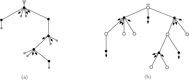
Figure 5. (a) A blossoming tree. (b) The corresponding rooted bipartite mobile.

Definition 8 (Blossoming trees).

A planted plane tree is a plane tree with a marked leaf; classically it is drawn in a top-down way; each vertex $v$ (different from the root-leaf) has $i$ (ordered) children, and the integer $i$ is called the arity of $v$. Vertices that are not leaves are colored black (so a black vertex means a vertex that is not a leaf). A blossoming tree is a rooted plane tree where each black vertex $v$, of arity $i\geq 1$, carries additionally $i-1$ dangling half-edges called buds (leaves carry no bud). The degree of such a black vertex $v$ is considered to be $2i$.

By a decomposition at the root, the generating function $T:=T(t;x_{1},x_{2},\dots)$ of blossoming trees, where $t$ marks the number of non-root leaves and $x_{i}$ marks the number of black vertices of degree $2i$, is given by:

(10) $$T=t+\sum_{i\geq 1}x_{i}\binom{2i-1}{i}T^{i}.$$

Claim 9.

There is a bijection between the family $\mathcal{T}$ of blossoming trees and the family $\mathcal{R}$ of rooted bipartite mobiles. For $\gamma\in\mathcal{T}$ and $\gamma^{\prime}\in\mathcal{R}$ the associated rooted bipartite mobile, each non-root leaf of $\gamma$ corresponds to a white vertex of $\gamma^{\prime}$, and each black vertex of degree $2i$ in $\gamma$ corresponds to a black vertex of degree $2i$ in $\gamma^{\prime}$.

Proof.

Note that the decomposition-equation (10) satisfied by $T$ is exactly the same as the decomposition-equation (2) satisfied by $R$. Hence $T=R$, and one can easily produce recursively a bijection between $\mathcal{T}$ and $\mathcal{R}$ that sends black vertices of degree $2i$ to black vertices of degree $2i$, and sends leaves to white vertices, for instance Figure 5 shows a blossoming tree and the corresponding rooted bipartite mobile. ∎

The bijection between $\mathcal{T}$ and $\mathcal{R}$ will be used in order to get rid of the black path (between the two black vertices of odd degrees) which appears in a quasi-bipartite mobile. Note that, if we denote by $\mathcal{R}^{\prime}$ the family of rooted mobiles with a marked white vertex (which does not contribute to the number of white vertices), and by $\mathcal{T}^{\prime}$ the family of blossoming trees with a marked non-root leaf (which does not contribute to the number of non-root leaves), then $\mathcal{T}^{\prime}\simeq\mathcal{R}^{\prime}$.

Let $\tau$ be a mobile with two marked black vertices $v_{1},v_{2}$. Let $P=(e_{1},\dots,e_{k})$ be the path between $v_{1}$ and $v_{2}$ in $\tau$. If we untie $e_{1}$ from $v_{1}$ and $e_{k}$ from $v_{2}$, we obtain 3 connected components: the one containing $P$ is called the middle-part $\tau^{\prime}$ of $\tau$; the edges $e_{1}$ and $e_{k}$ are called respectively the first end and the second end of $\tau^{\prime}$ in $\tau$. The vertices $v_{1}$ and $v_{2}$ are called extremal.

Let $\mathcal{H}$ be the family of structures that can be obtained as middle-parts of quasi-bipartite mobiles where $v_{1}$ and $v_{2}$ are the two black vertices of odd degree (hence the path between $v_{1}$ and $v_{2}$ contains only black vertices). And let $\mathcal{K}$ be the family of structures that can be obtained as middle-parts of bipartite mobiles with two marked black vertices $v_{1},v_{2}$.

Lemma 10.

We have the following bijections:

$$\mathcal{H}\simeq\mathcal{T}^{\prime}\simeq\mathcal{R}^{\prime}\hskip 85.35826pt\mathcal{K}\simeq\mathcal{R}^{\prime}\times\mathcal{R}$$

Hence:

$\mathcal{K}\simeq\mathcal{H}\times\mathcal{R}$.

In these bijections each non-extremal black vertex of degree $2i$ in an object on the left-hand side corresponds to a non-extremal black vertex of degree $2i$ in the corresponding object on the right-hand side.

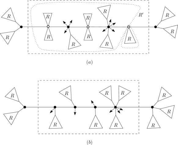
Figure 6. middle-parts in the bipartite case $(a)$ and in the quasi-bipartite case $(b)$.

Proof.

Note that any $\tau\in\mathcal{H}$ consists of a path $P$ of black vertices, and each vertex of degree $2i$ in $P$ carries (outside of $P$) $i-1$ buds and $i-1$ rooted mobiles (in $\mathcal{R}$), as illustrated in Figure 6(b). Let $\tau^{\prime}$ be $\tau$ where each rooted mobile attached to $P$ is replaced by the corresponding blossoming tree (using the isomorphism of Claim 9), and where the ends of $\gamma$ are considered as two marked leaves (respectively the root-leaf and a marked non-root leaf). We clearly have $\tau^{\prime}\in\mathcal{T}^{\prime}$. Conversely, starting from $\tau^{\prime}\in\mathcal{T}^{\prime}$, let $P$ be the path between the root-leaf and the non-root marked leaf. Each vertex of degree $2i$ on $P$ carries (outside of $P$) $i-1$ buds and $i-1$ blossoming trees. Replacing each blossoming tree attached to $P$ by the corresponding rooted mobile, and seeing the two marked leaves as the first and second end of $P$, one gets a structure in $\mathcal{H}$. So we have $\mathcal{H}\simeq\mathcal{T}^{\prime}$.

The bijection $\mathcal{K}\simeq\mathcal{R}^{\prime}\times\mathcal{R}$ is simpler. Indeed, any $\tau\in\mathcal{K}$ can be seen as a rooted mobile $\gamma$ with a secondary marked corner at a white vertex (see Figure 6(a)). Let $w$ (resp. $w^{\prime}$) be the white vertex at the root (resp. at the secondary marked corner) and let $P$ be the path between $w$ and $w^{\prime}$. Each white vertex on $P$ can be seen as carrying two rooted mobiles (in $\mathcal{R}$), one on each side of $P$. Let $r,r^{\prime}$ be the two rooted mobiles attached at $w^{\prime}$ (say, $r$ is the one on the left of $w^{\prime}$ when looking toward $w$). If we untie $r$ from the rest of $\gamma$, then $w^{\prime}$ now just acts as a marked white vertex in $\gamma$, so the pair $(\gamma,r)$ is in $\mathcal{R}^{\prime}\times\mathcal{R}$. The mapping from $(\gamma,r)\in\mathcal{R}^{\prime}\times\mathcal{R}$ to $\tau\in\mathcal{K}$ processes in the reverse way. We get $\mathcal{K}\simeq\mathcal{R}^{\prime}\times\mathcal{R}$. ∎

At the level of generating function expressions, Lemma 10 has been proved by Chapuy [9, Prop.7.5] in an even more precise form (which keeps track of a certain distance-parameter between the two extremities). We include our own proof to make the paper self-contained, and because the new idea of using blossoming trees as auxiliary tools yields a short bijective proof.

Now from Lemma 10 we can deduce a reduction from the quasi-bipartite to the bipartite case (in Lemma 11 thereafter, see also Figure 6). Let $a_{1}$ and $a_{2}$ be positive integers. Define $\mathcal{B}_{2a_{1},2a_{2}}$ as the family of bipartite mobiles with two marked black vertices $v_{1},v_{2}$ of respective degrees $2a_{1},2a_{2}$. Similarly, define $\mathcal{Q}_{2a_{1}-1,2a_{2}+1}$ as the family of quasi-bipartite mobiles with two marked black vertices $v_{1},v_{2}$ of respective degrees $2a_{1}-1,2a_{2}+1$ (i.e., the marked vertices are the two black vertices of odd degree). Let $\widehat{\mathcal{B}}_{2a_{1},2a_{2}}$ be the family of pruned mobiles (recall that “pruned” means “where buds at marked black vertices are taken out”) obtained from mobiles in $\mathcal{B}_{2a_{1},2a_{2}}$, and let $\widehat{\mathcal{Q}}_{2a_{1}-1,2a_{2}+1}$ be the family of pruned mobiles obtained from mobiles in $\mathcal{Q}_{2a_{1}-1,2a_{2}+1}$.

Lemma 11.

For $a_{1},a_{2}$ two positive integers:

$$\widehat{\mathcal{B}}_{2a_{1},2a_{2}}\simeq\widehat{\mathcal{Q}}_{2a_{1}-1,2a_{2}+1}.$$

In addition, if $\gamma\in\widehat{\mathcal{B}}_{2a_{1},2a_{2}}$ corresponds to $\gamma^{\prime}\in\widehat{\mathcal{Q}}_{2a_{1}-1,2a_{2}+1}$, then each non-marked black vertex of degree $2i$ (resp. each white vertex) in $\gamma$ corresponds to a non-marked black vertex of degree $2i$ (resp. to a white vertex) in $\gamma^{\prime}$.

Proof.

Let $\gamma\in\widehat{\mathcal{Q}}_{2a_{1}-1,2a_{2}+1}$, and let $\tau$ be the middle-part of $\gamma$. We construct $\gamma^{\prime}\in\widehat{\mathcal{B}}_{2a_{1},2a_{2}}$ as follows. Note that $v_{2}$ has a black neighbour $b$ (along the branch from $v_{2}$ to $v_{1}$) and has otherwise $a_{2}$ white neighbours. Let $w$ be next neighbour after $b$ in counter-clockwise order around $v_{2}$, and let $r$ be the mobile (in $\mathcal{R}$) hanging from $w$. According to Lemma 10, the pair $(\tau,r)$ corresponds to some $\tau^{\prime}\in\mathcal{K}$. If we replace the middle-part $\tau$ by $\tau^{\prime}$ and take out the edge $\{v_{2},w\}$ and the mobile $r$, we obtain some $\gamma^{\prime}\in\widehat{\mathcal{B}}_{2a_{1},2a_{2}}$. The inverse process is easy to describe, so we obtain a bijection between $\widehat{\mathcal{Q}}_{2a_{1}-1,2a_{2}+1}$ and $\widehat{\mathcal{B}}_{2a_{1},2a_{2}}$. ∎

Lemma 11 (in an equivalent form) has first been shown by Cori [11, Theo.VI p.75] (again we have provided our own short proof to be self-contained).

As a corollary of Lemma 11, we obtain the formula of Theorem 1 in the quasi-bipartite case, with the exception of the case where the two odd boundaries are of length $1$ (this case will be treated later, in Lemma 13).

Corollary 12.

For $r\geq 2$ and $a_{1},\ldots,a_{r}$ positive integers, the generating function $G_{2a_{1}-1,2a_{2}+1,2a_{3},\dots,2a_{r}}$ satisfies (5).

Proof.

We first consider the case $r=2$. Let $\widehat{B}_{2a_{1},2a_{2}}=\widehat{B}_{2a_{1},2a_{2}}(t;x_{1},x_{2},\ldots)$ (resp. $B_{2a_{1},2a_{2}}=B_{2a_{1},2a_{2}}(t;x_{1},x_{2},\ldots)$) be the generating function of $\widehat{\mathcal{B}}_{2a_{1},2a_{2}}$ (resp. of $\mathcal{B}_{2a_{1},2a_{2}}$) where $t$ marks the number of white vertices and $x_{i}$ marks the number of non-marked black vertices of degree $2i$. There are $\binom{2a_{i}-1}{a_{i}}$ ways to place the buds at each marked black vertex $v_{i}$ ($i\in\{1,2\}$), hence:

$$B_{2a_{1},2a_{2}}=\binom{2a_{1}-1}{a_{1}}\binom{2a_{2}-1}{a_{2}}\widehat{B}_{2a_{1},2a_{2}}.$$

In addition Theorem 4 ensures that $G_{2a_{1},2a_{2}}\ \!\!^{\prime}=2a_{1}2a_{2}B_{2a_{1},2a_{2}}$ (the multiplicative factor being due to the choice of a marked corner in each boundary-face). Hence:

$$G_{2a_{1},2a_{2}}\ \!\!^{\prime}=4a_{1}a_{2}\binom{2a_{1}-1}{a_{1}}\binom{2a_{2}-1}{a_{2}}\widehat{B}_{2a_{1},2a_{2}}.$$

Similarly, if we denote by $\widehat{Q}_{2a_{1}-1,2a_{2}+1}=\widehat{Q}_{2a_{1}-1,2a_{2}+1}(t;x_{1},x_{2},\ldots)$ the generating function of the family $\widehat{\mathcal{Q}}_{2a_{1}-1,2a_{2}+1}$ where $t$ marks the number of white vertices and $x_{i}$ marks the number of non-marked black vertices of degree $2i$, then we have:

$$G_{2a_{1}-1,2a_{2}+1}\ \!\!^{\prime}=(2a_{1}-1)(2a_{2}+1)\binom{2a_{1}-2}{a_{1}-1}\binom{2a_{2}}{a_{2}}\widehat{Q}_{2a_{1}-1,2a_{2}+1}.$$

Since $\widehat{B}_{2a_{1},2a_{2}}=\widehat{Q}_{2a_{1}-1,2a_{2}+1}$ by Lemma 11, we get (with the notation $\alpha(\ell)=\displaystyle{\tfrac{\ell!}{\lfloor\ell/2\rfloor!\lfloor(\ell-1)/2\rfloor!}}$):

$$\alpha(2a_{1}-1)\cdot\alpha(2a_{2}+1)\cdot G_{2a_{1},2a_{2}}=\alpha(2a_{1})\cdot\alpha(2a_{2})\cdot G_{2a_{1}-1,2a_{2}+1}.$$

In a very similar way (by the isomorphism of Lemma 11), we have for $r\geq 2$:

$$\alpha(2a_{1}-1)\cdot\alpha(2a_{2}+1)\cdot G_{2a_{1},2a_{2},2a_{3},\ldots,2a_{r}}=\alpha(2a_{1})\cdot\alpha(2a_{2})\cdot G_{2a_{1}-1,2a_{2}+1,2a_{3},\ldots,2a_{r}}.$$

Hence the fact that $G_{2a_{1}-1,2a_{2}+1,2a_{3},\ldots,2a_{r}}$ satisfies (5) follows from the fact (already proved in Corollary 7) that $G_{2a_{1},2a_{2},2a_{3},\ldots,2a_{r}}$ satisfies (5). ∎

It remains to show the fomula when the two odd boundary-faces have length $1$. For that case, we have the following counterpart of Lemma 11:

Lemma 13.

Let $\mathcal{B}_{2}$ be the family of bipartite mobiles with a marked black vertex of degree $2$, and let $\mathcal{B}_{2}^{\prime}$ be the family of objects from $\mathcal{B}_{2}$ where a white vertex is marked. Then

$$\mathcal{Q}_{1,1}\simeq\mathcal{B}_{2}^{\prime}.$$

In addition, if $\gamma\in\mathcal{B}_{2}^{\prime}$ corresponds to $\gamma^{\prime}\in\mathcal{Q}_{1,1}$, then each white vertex of $\gamma$ corresponds to a white vertex of $\gamma^{\prime}$, and each non-marked black vertex of degree $2i$ in $\gamma$ corresponds to a non-marked black vertex of degree $2i$ in $\gamma^{\prime}$.

Proof.

A mobile in $\mathcal{Q}_{1,1}$ is completely reduced to its middle-part, so we have

$$\mathcal{Q}_{1,1}\simeq\mathcal{H}\simeq\mathcal{T}^{\prime}\simeq\mathcal{R}^{\prime}.$$

Consider a mobile in $\mathcal{R}^{\prime}$, i.e., a bipartite mobile where a corner incident to a white vertex is marked, and a secondary white vertex is marked. At the marked corner we can attach an edge connected to a new marked black vertex $b$ of degree $2$ (the other incident half-edge of $b$ being a bud). We thus obtain a mobile in $\mathcal{B}_{2}^{\prime}$, and the mapping is clearly a bijection. ∎

By Lemma 13 we have $2\ \!G_{1,1}=G_{2}^{\prime}$, and similarly $2\ \!G_{1,1,2a_{3},\ldots,2a_{r}}=G_{2,2a_{3},\ldots,2a_{r}}\ \!\!^{\prime}$. Hence, again the fact that $G_{1,1,2a_{3},\ldots,2a_{r}}$ satisfies (5) follows from the fact that $G_{2,2a_{3},\ldots,2a_{r}}$ satisfies (5), which has been shown in Corollary 7.

5. Extension to $p$-constellations and quasi $p$-constellations

We show in this next section that the formula obtained for bipartite and quasi-bipartite maps (Theorem 1) naturally extends to a formula (Theorem 2) for $p$-constellations and quasi $p$-constellations. The ingredients are the same (bijection with mobiles and aggregation process to get the formula for $p$-constellations, and then use blossoming trees to reduce the formula for quasi $p$-constellations to the formula for $p$-constellations).

5.1. Bijection between vertex-pointed hypermaps and hypermobiles

Hypermaps admit a natural orientation by orienting each edge so as to have its incident dark face to its left. The following bijection is again a reformulation of the bijection in [7] between vertex-pointed eulerian maps and mobiles. Starting from a hypermap $G$ with a pointed vertex $v_{0}$, and where the vertices of $G$ are considered as round vertices, one obtains a mobile $M$ as follows:

• Endow $G$ with its natural orientation.

• Endow $G$ with its geodesic orientation by keeping oriented edges which belong to a geodesic oriented path from $v_{0}$.

• Label vertices of $G$ by their distance from $v_{0}$.

• Put a light (resp. dark) square in each light (resp. dark) face of $G$.

• Apply the following rules to each edge (oriented or not) of $G$:

  

• Forget labels on vertices.

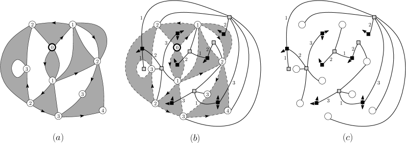
Figure 7. (a) A vertex-pointed hypermap endowed with its geodesic orientation (with respect to the marked vertex). (b) The local rule is applied to each edge of the hypermap. (c) The resulting hypermobile.

Definition 14 (Hypermobiles).

A hypermobile is a tree with three types of vertices (round, dark square, and light square) and positive integers (called weights) on some edges, such that:

• there are two types of edges: between a round vertex and a light square vertex, or between a dark square vertex and a light square vertex (these edges are called dark-light edges),

• dark square vertices possibly carry buds,

• dark-light edges carry a strictly positive weight, such that, for each square vertex (dark or light), the sum of weights on its incident edges equals the degree of the vertex.

Theorem 15 (Bouttier, Di Francesco and Guitter [7]).

The above construction is a bijection between vertex-pointed hypermaps and hypermobiles. Each non-pointed vertex in the hypermap corresponds to a round vertex in the associated hypermobile, and each dark (resp. light) face corresponds to a dark (resp. light) square vertex of the same degree in the associated hypermobile.

5.2. Proof of Theorem 2 for $p$-constellations

For $p\geq 2$, hypermobiles corresponding to vertex-pointed $p$-constellations are called $p$-mobiles.

Claim 16 (Characterization of $p$-mobiles [7]).

A $p$-mobile satisfies the following properties:

• dark-light edges have weight $p$,

• each dark square vertex, of degree $p$, has one light square neighbour and $p-1$ buds (thus can be seen as a “big bud” attached to the light square neighbour),

• each light square vertex, of degree $pi$ for some $i\geq 1$, has $i$ dark square neighbours (i.e., carries $i$ big buds) and $(p-1)i$ round neighbours.

Proof.

The first assertion is proved as follows. Let $T$ be a $p$-mobile and $F$ the forest formed by the edges whose weight is not a multiple of $p$, and their incident vertices. By construction, for each vertex of $T$, the degree and the sum of weights are multiple of $p$. Assume $F$ is non-empty. Then $F$ has a leaf $v$. Hence $v$ has a unique incident edge whose weight is not a multiple of $p$, which implies that the degree of $p$ is not a multiple of $p$, a contradiction. Hence $F$ is empty and each weight in $T$ is a multiple of $p$. Moreover, dark square vertices have degree $p$, which implies that weights are at most equal to $p$. Hence all weights are equal to $p$. Then the second and third assertion follow directly from the first one. ∎

Since the weights are always $p$ they can be omitted, and seeing dark square vertices as “big buds” it is clear that in the case $p=2$ we recover the mobiles for bipartite maps. A rooted $p$-mobile is a $p$-mobile with a marked corner at a round vertex. Let $R_{p}\equiv R_{p}(t)\equiv R_{p}(t;x_{1},x_{2},\ldots)$ be the generating function of rooted $p$-mobiles where $t$ marks the number of white vertices and, for $i\geq 1$, $x_{i}$ marks the number of light square vertices of degree $pi$. By a decomposition at the root (see [7]), $R_{p}$ satisfies (6).

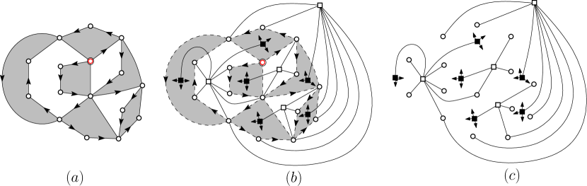
Figure 8. (a) A vertex-pointed $p$-constellation, $p=4$, endowed with its geodesic orientation (with respect to the marked vertex). (b) The local rule is applied to each edge of the map. (c) The resulting $p$-mobile (weights on dark-light edges, which all equal $p$, are omitted).

One can now use the same processus as in Section 3 to describe $p$-constellations with $r$ boundaries. For a $p$-mobile $\gamma$ with marked light square vertices $b_{1},\ldots,b_{r}$ of degrees $pa_{1},\ldots,pa_{r}$, the associated pruned $p$-mobile $\widehat{\gamma}$ is obtained from $\gamma$ by deleting the (big) buds at the marked vertices (thus the marked vertices get degrees $(p-1)a_{1},\ldots,(p-1)a_{r}$). Conversely, such a pruned mobile yields $\prod_{i=1}^{r}{pa_{i}-1\choose a_{i}}$ mobiles (because of the number of ways to place the big buds around the marked light square vertices). Hence, if we denote by $\mathcal{B}^{(p)}_{pa_{1},\dots,pa_{r}}$ the family of $p$-mobiles with $r$ marked light square vertices of respective degrees $pa_{1},\dots,pa_{r}$, and denote by $\widehat{\mathcal{B}}_{pa_{1},\dots,pa_{r}}^{(p)}$ the family of pruned $p$-mobiles with $r$ marked light square vertices of respective degree $(p-1)a_{1},\dots,(p-1)a_{r}$, we have:

$$\mathcal{B}^{(p)}_{pa_{1},\dots,pa_{r}}\simeq\prod_{i=1}^{r}{pa_{i}-1\choose a_{i}}\widehat{\mathcal{B}}^{(p)}_{pa_{1},\dots,pa_{r}}$$

We consider the two following families:

• $\widehat{\mathcal{M}}^{(p)}_{pa_{1},\dots,pa_{r}}$ is the family of pruned $p$-mobiles with $r$ marked light square vertices $v_{1},\ldots,v_{r}$ of respective degrees $(p-1)a_{1},\dots,(p-1)a_{r}$, the mobile being rooted at a corner of one of the marked vertices,

• $\mathcal{F}^{(p)}_{s}$ is the family of forests made of $s:=(p-1)\sum_{i=1}^{r}a_{i}$ rooted $p$-mobiles, and where additionnally $r-1$ round vertices $w_{1},\ldots,w_{r-1}$ are marked.

Proposition 17.

There is an $(r-1)!$-to-$(r-1)!$ correspondence between the family $\widehat{\mathcal{M}}^{(p)}_{pa_{1},\dots,pa_{r}}$ and the family $\mathcal{F}^{(p)}_{s}$. If $\gamma\in\widehat{\mathcal{M}}^{(p)}_{pa_{1},\dots,pa_{r}}$ corresponds to $\gamma^{\prime}\in\mathcal{F}^{(p)}_{s}$, then each round vertex in $\gamma$ corresponds to a round vertex in $\gamma^{\prime}$, and each light square vertex of degree $pi$ in $\gamma$ corresponds to a light square vertex of degree $pi$ in $\gamma^{\prime}$.

Proof.

This correspondence works in the same way as in Theorem 6, where light square vertices act as black vertices and round vertices act as white vertices, and where one groups the first $(p-1)a_{1}$ components of the forest, then the following $(p-1)a_{2}$ components, and so on, and then uses the same aggregation process as in the bipartite case. ∎

As a corollary we obtain the formula of Theorem 2 in the case of $p$-constellations:

Corollary 18.

For $r\geq 1$ and $a_{1},\ldots,a_{r}$ positive integers, the generating function $G^{(p)}_{pa_{1},\ldots,pa_{r}}$ satisfies:

(11) $$G^{(p)}_{pa_{1},\dots,pa_{r}}=\left(\prod_{i=1}^{r}\frac{(pa_{i})!}{((p-1)a_{i}-1)!a_{i}!}\right)\cdot\frac{1}{s}\cdot\frac{\mathrm{d}^{r-\!2}}{\mathrm{d}t^{r-\!2}}R_{p}^{s},\ \ \mathrm{where}\ s=(p-1)\sum_{i=1}^{r}a_{i}.$$

Proof.

In the case $r=1$, the expression reads $G^{(p)}_{pa}\ \!\!{}^{\prime}=\binom{pa}{a}R_{p}^{a}$, which is a direct consequence of the bijection with $p$-mobiles (indeed $G^{(p)}_{pa}\ \!\!{}^{\prime}$ is the series of $p$-mobiles with a marked light square vertex $v$ of degree $pa$, with a marked corner incident to $v$). So we now assume $r\geq 2$. The formula derives (as formula (9)) by combining the bijection of Theorem 15 and the correspondence of Proposition 17, upon consistent rooting and placing of the buds, and a final integration.

∎

5.3. Proof of Theorem 2 for quasi $p$-constellations

In a similar way as for quasi bipartite maps, we prove Theorem 2 in the case of quasi $p$-constellations (two boundaries have length not a multiple of $p$) by a reduction to $p$-constellations, with some more technical details. We call quasi $p$-mobiles the hypermobiles associated to quasi $p$-constellations by the bijection of Section 5.1, see Figure 9 for an example. In the following, we will refer to vertices whose degree is not a multiple of $p$ as non-regular vertices and edges whose weight is not a multiple of $p$ as non-regular edges.

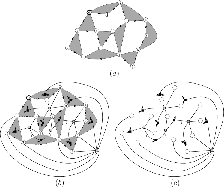
Figure 9. (a) A vertex-pointed quasi-$3$-constellation endowed with the geodesic orientation. (b) The local rule is applied to each edge of the map. (c) The resulting quasi-$3$-mobile, where the weights on the alternating path are $(1,2,1,2)$.

Claim 19 (Alternating path in a quasi-$p$-mobile).

In a quasi-$p$-mobile, all weights of edges are at most $p$ (so regular edges have weight $p$) and the set of non-regular edges forms a non-empty path whose extremities are the two non-regular vertices. Moreover, if the degrees of the non-regular vertices $v_{1},v_{2}$ are $pi-d=p(i-1)+p-d$ and $pj+d,~{}i,j\geq 1,~{}1\leq d\leq p-1$ (the sum of the two degrees must be a multiple of $p$), the weights along the path from $v_{1}$ to $v_{2}$ start with $p-d$, alternate between $p-d$ and $d$, and end with $d$.

Proof.

The fact that the weights are at most $p$ just follows from the fact that dark square vertices have degree $p$. Let $T$ be a quasi-$p$-mobile, and let $F$ be the forest formed by the non-regular edges of $T$. Leaves of $F$ are necessarily non-regular, hence $F$ has only two leaves which are $v_{1},v_{2}$, so $F$ is reduced to a path $P$ connecting $v_{1}$ and $v_{2}$. Starting from $v_{1}$, the first edge of $P$ must have weight $p-d$. This edge is incident to a black square vertex of degree $p$, so the following edge of $P$ must have weight $d$. The next vertex on $P$ is either $v_{2}$ or is a regular light square vertex, in which case the next edge along $P$ must have weight $p-d$. The alternation continues the same way until reaching $v_{2}$ (necessarily using an edge of weight $d$). ∎

As for $p$-mobiles, weights on regular edges (always equal to $p$) can be omitted, and dark square vertices not on the alternating path can be seen as “big buds” (those on the alternating path are considered as “intermediate” dark square vertices). It is easy to check that regular light square vertices of degree $pi$ are adjacent to $i$ big buds, and non-regular light square vertices of degree $pi+d$ (for some $1\leq d\leq p-1$) are adjacent to $i$ big buds.

Definition 20 (Blossoming $p$-trees [4]).

For $p\geq 2$, a planted $p$-tree is a planted tree (non-leaf vertices are light square, leaves are round) where the arity of internal vertices is of the form $(p-1)i$. A blossoming $p$-tree is a structure obtained from a planted $p$-tree where:

• on each edge going down to a light square vertex, a dark square vertex (called intermediate) is inserted that additionally carries $p-2$ buds,

• at each light square vertex of arity $(p-1)i$ one further attaches $i-1$ new dark square vertices (called big buds), each such dark square vertex carrying additionally $p-1$ buds. (After these attachments, the light square vertex is considered to have degree $pi$.)

Figure 10. A blossoming $4$-tree.

Note that in a blossoming $p$-tree, dark square vertices have degree $p$. When $p=2$, dark square vertices can be erased, and we obtain the description of a standard blossoming tree. By a decomposition at the root [4], the generating function $T_{p}:=T_{p}(t;x_{1},x_{2},\dots)$ of rooted blossoming $p$-trees, where $t$ marks the number of non-root (round) leaves and $x_{i}$ marks the number of light square vertices of degree $pi$, is given by:

(12) $$T_{p}=t+\sum_{i\geq 1}(p-1)\cdot x_{i}\binom{pi-1}{i-1}T_{p}^{(p-1)i}=t+\sum_{i\geq 1}x_{i}\binom{pi-1}{i}T_{p}^{(p-1)i},$$

where the factor $(p-1)$ in the sum represents the number of ways to place the $(p-2)$ buds at the dark square vertex adjacent to the root.

Claim 21.

There is a bijection between the family $\mathcal{T}_{p}$ of blossoming $p$-trees and the family $\mathcal{R}_{p}$ of rooted $p$-mobiles. For $\gamma\in\mathcal{T}_{p}$ and $\gamma^{\prime}\in\mathcal{R}_{p}$ the associated rooted $p$-mobile, each non-root round leaf of $\gamma$ corresponds to a round vertex of $\gamma^{\prime}$, each light square vertex of degree $pi$ in $\gamma$ corresponds to a light square vertex of degree $pi$ in $\gamma^{\prime}$.

Proof.

Note that the decomposition-equation (12) satisfied by $T_{p}$ is exactly the same as the decomposition-equation (6) satisfied by $R_{p}$. Hence $T_{p}=R_{p}$, and one can easily produce recursively a bijection between $\mathcal{T}_{p}$ and $\mathcal{R}_{p}$ that sends light square vertices of degree $pi$ to light square vertices of degree $pi$, and sends non-root round leaves to round vertices. ∎

The bijection between $\mathcal{T}_{p}$ and $\mathcal{R}_{p}$ will be used in order to get rid of the alternating path between the non-regular two light square vertices that appear in a quasi-$p$-mobile. Note that, if we denote by $\mathcal{R}_{p}^{\prime}$ the family of rooted $p$-mobiles with a marked round vertex (which does not contribute to the number of round vertices), and by $\mathcal{T}_{p}^{\prime}$ the family of blossoming $p$-trees with a marked round leaf (which does not contribute to the number of round leaves), then $\mathcal{T}_{p}^{\prime}\simeq\mathcal{R}_{p}^{\prime}$.

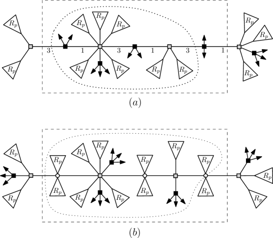
Figure 11. Middle-parts in a quasi-$4$-mobile $(a)$, and in a $4$-mobile $(b)$.

As in the (quasi-) bipartite case, for a hypermobile with two marked light-square vertices $v_{1},v_{2}$, we can consider the operation of untying the two ends of the path $P$ connecting $v_{1}$ and $v_{2}$. The obtained structure (taking away the connected components not containing $P$) is called the middle-part of the hypermobile. Let $\mathcal{H}_{p}$ be the family of structures that can be obtained as middle-parts of quasi-$p$-mobiles, where $v_{1}$ and $v_{2}$ are the two (ordered) non-regular vertices (thus $P$ is the alternating path of the quasi $p$-mobile). And let $\mathcal{K}_{p}$ be the family of structures that can be obtained as middle-parts of $p$-mobiles with two marked light square vertices $v_{1},v_{2}$. In the case of $\mathcal{H}_{p}$, note that, according to Claim 21, the weights along the alternating path only depend on the degrees (modulo $p$) of the end vertices. In particular, the shape of the middle-part and the labels along the path are independent. Hence, from now on the weights can be omitted when considering middle-parts from $\mathcal{H}_{p}$.

Lemma 22.

We have the following bijections:

$$\mathcal{H}_{p}\simeq(p-1)\cdot\mathcal{T}_{p}^{\prime}\simeq(p-1)\cdot\mathcal{R}_{p}^{\prime}\hskip 85.35826pt\mathcal{K}_{p}\simeq\mathcal{R}_{p}^{\prime}\times\mathcal{R}_{p}$$

Hence:

$(p-1)\cdot\mathcal{K}_{p}\simeq\mathcal{H}_{p}\times\mathcal{R}_{p}$.

In these bijections, each light square vertex of degree $pi$ in an object on the left-hand side corresponds to a light square vertex of degree $pi$ in the corresponding object on the right-hand side.

Proof.

For $\mathcal{K}_{p}\simeq\mathcal{R}_{p}^{\prime}\times\mathcal{R}_{p}$, the proof is similar to Lemma 10, see Figure 11(b). To prove $\mathcal{H}_{p}\simeq(p-1)\cdot\mathcal{T}_{p}^{\prime}$ (see also Figure 11(a)), we start similarly as in the proof of Lemma 10, replacing each rooted $p$-mobile “adjacent” to the alternating path $P$ by the corresponding blossoming $p$-tree. Let $b$ be the (intermediate) dark square vertex adjacent to $v_{2}$ on $P$. If we erase the $p-2$ buds at $b$, then we naturally obtain a structure in $\mathcal{T}_{p}^{\prime}$ ($b$ acts as a secondary marked leaf once its incident buds are taken out). Conversely there are $p-1$ ways to distribute the buds at $b$, which gives a factor $p-1$. ∎

Again, at the level of generating function expressions, an even more precise statement (keeping track of a certain distance parameter between the two marked vertices) is given by Chapuy [9, Prop.7.5] (we include our quite shorter and completely bijective proof to make the paper self-contained).

Now from Lemma 22 we reduce pruned quasi-$p$-mobiles to pruned $p$-mobiles (pruned means: big buds at the marked light square vertices are taken out). Let $a_{1},a_{2}$ be positive integers, and $1\leq d\leq p-1$. Define $\widehat{\mathcal{B}}^{(p)}_{pa_{1},pa_{2}}$ as the family of pruned $p$-mobiles with two marked black vertices $v_{1},v_{2}$ of respective degrees $(p-1)a_{1},(p-1)a_{2}$. Similarly define $\widehat{\mathcal{Q}}^{(p)}_{pa_{1}-d,pa_{2}+d}$ as the family of pruned quasi-$p$-mobiles with two marked black vertices $v_{1},v_{2}$ of respective degrees $(p-1)a_{1}-d+1,(p-1)a_{2}+d$ (the two marked light square vertices are the non-regular ones).

Lemma 23.

For $a_{1},a_{2}$ two positive integers, and $1\leq d\leq p-1$:

$$(p-1)\cdot\widehat{\mathcal{B}}^{(p)}_{pa_{1},pa_{2}}\simeq\widehat{\mathcal{Q}}^{(p)}_{pa_{1}-d,pa_{2}+d}.$$

In addition, if $\gamma\in\widehat{\mathcal{B}}^{(p)}_{pa_{1},pa_{2}}$ corresponds to $\gamma^{\prime}\in\widehat{\mathcal{Q}}^{(p)}_{pa_{1}-d,pa_{2}+d}$, then each non-marked light square vertex of degree $pi$ in $\gamma$ corresponds to a non-marked light square vertex of degree $pi$ in $\gamma^{\prime}$.

Proof.

The proof is similar to Lemma 11, where we additionally have to transfer a part of the degree contribution from one end of the alternating path to the other, in order to obtain a well-formed pruned $p$-mobile. Let $\gamma\in\widehat{\mathcal{Q}}^{(p)}_{pa_{1}-d,pa_{2}+d}$, and let $\tau$ be the middle-part of $\gamma$. We construct $\gamma^{\prime}\in\widehat{\mathcal{B}}^{(p)}_{pa_{1},pa_{2}}$ as follows. Note that $v_{2}$ has a dark square neighbour $b$ (along the path from $v_{2}$ to $v_{1}$) and has otherwise $(p-1)a_{2}+d-1$ white neighbours. Let $w_{0},\dots,w_{d-1}$ be the $d$ next neighbourd after $b$ in counter-clockwise order around $v_{2}$, and let $r_{0},\dots,r_{d-1}$ be the mobiles (in $\mathcal{R}_{p}$) hanging from $w_{0},\dots,w_{d-1}$. According to Lemma 10, the pair $(\tau,r_{0})$ corresponds to some pair $(i,\tau^{\prime})$, where $1\leq i\leq p-1$ and $\tau^{\prime}\in\mathcal{K}_{p}$. If we replace the middle-part $\tau$ by $\tau^{\prime}$ and take out the edge $\{v_{2},w_{0}\}$ and the mobile $r_{0}$, then transfer $r_{1},\dots,r_{d-1}$ from $v_{2}$ to $v_{1}$, we obtain some $\gamma^{\prime}\in\widehat{\mathcal{B}}^{(p)}_{pa_{1},pa_{2}}$. We associate to $\gamma$ the pair $(i,\gamma^{\prime})$. The inverse process is easy to describe, so we obtain a bijection between $\widehat{\mathcal{Q}}^{(p)}_{pa_{1}-d,pa_{2}+d}$ and $(p-1)\cdot\widehat{\mathcal{B}}^{(p)}_{pa_{1},pa_{2}}$. ∎

Denote by $\mathcal{Q}_{pa_{1}-d_{1},pa_{2}+d,pa_{3},\ldots,pa_{r}}$ the family of quasi $p$-constellations where the marked light faces are of degrees $pa_{1}-d,pa_{2}+d,pa_{3},\ldots,pa_{r}$. As a corollary of Lemma 23 (the additionnal factors correspond to the number of ways to place the big buds at the pruned marked vertices), we obtain

$${pa_{1}-1\choose a_{1}}{pa_{2}-1\choose a_{2}}\mathcal{Q}^{(p)}_{pa_{1}-d,pa_{2}+d}\simeq(p-1)\cdot{pa_{1}-d-1\choose a_{1}-1}{pa_{2}+d-1\choose a_{2}}\mathcal{B}^{(p)}_{pa_{1},pa_{2}},$$

and very similarly (since the isomorphism of Lemma 23 preserves light square vertex degrees):

$${pa_{1}-1\choose a_{1}}{pa_{2}-1\choose a_{2}}\mathcal{Q}^{(p)}_{pa_{1}-d,pa_{2}+d,pa_{3},\ldots,pa_{r}}\simeq(p-1)\cdot{pa_{1}-d-1\choose a_{1}-1}{pa_{2}+d-1\choose a_{2}}\mathcal{B}^{(p)}_{pa_{1},pa_{2},pa_{3},\ldots,pa_{r}},$$

which yields Theorem 2 in the case where at least one of the two non-regular (degree not multiple of $p$) light faces is of degree larger than $p$. In the remaining we show the formula of Theorem 2 when the two non-regular light faces are of degree smaller than $p$.

Lemma 24.

Let $\mathcal{B}_{p}$ be the family of $p$-mobiles with a marked light square vertex of degree $p$, and let $\mathcal{B}_{p}^{\prime}$ be the family of objects from $\mathcal{B}_{p}$ where a round vertex is marked. Then, for any $d\in[1..p-1]$,

$$\mathcal{Q}^{(p)}_{d,p-d}\simeq\mathcal{B}_{p}^{\prime}.$$

In addition, if $\gamma\in\mathcal{B}_{p}^{\prime}$ corresponds to $\gamma^{\prime}\in\mathcal{Q}^{(p)}_{d,p-d}$, then each non-marked light square vertex of degree $pi$ in $\gamma$ corresponds to a non-marked light square vertex of degree $pi$ in $\gamma^{\prime}$.

Proof.

A mobile in $\mathcal{Q}^{(p)}_{d,p-d}$ can be decomposed as follows: two marked light squares $v_{1},v_{2}$, their incident rooted $p$-mobiles (one for each round neighbour) and the middle-part. Hence we have:

$$\mathcal{Q}^{(p)}_{d,p-d} \simeq \mathcal{R}_{p}^{d-1}\times\mathcal{H}_{p}\times\mathcal{R}_{p}^{p-d-1}$$

$$\simeq (p-1)\cdot\mathcal{T}_{p}^{\prime}\times\mathcal{R}_{p}^{p-2}$$

$$\simeq (p-1)\cdot\mathcal{R}_{p}^{\prime}\times\mathcal{R}_{p}^{p-2}.$$

If we now consider an object $\gamma^{\prime}\in\mathcal{B}_{p}^{\prime}$, the marked light square vertex (of degree $p$) carries one big bud, and has $p-1$ white neighbours $w_{1},\ldots,w_{p-1}$. From each white neighbour $w_{i}$ hangs a rooted $p$-mobile $r_{i}$, and one of these rooted $p$-mobiles has a secondary marked round vertex (the secondary marked vertex of $\gamma^{\prime}$). Thus

$$\mathcal{B}_{p}^{\prime}\simeq(p-1)\cdot\mathcal{R}_{p}^{\prime}\times\mathcal{R}_{p}^{p-2},$$

where the factor $p-1$ is due to the choice of which of the mobiles $r_{1},\ldots,r_{p-1}$ carries the secondary marked round vertex. ∎

By Lemma 24 we have:

$$p\ \!G^{(p)}_{d,p-d}=d(p-d)\ (G^{(p)}_{p})^{\prime},$$

(the additional factors are due to marking a corner in each marked light face), and similarly:

$$p\ \!G^{(p)}_{d,p-d,pa_{3},\ldots,pa_{r}}=d(p-d)\ G^{(p)}_{p,pa_{3},\ldots,pa_{r}}\ \!\!{}^{\prime}.$$

Hence, again the fact that $G^{(p)}_{d,p-d,pa_{3},\ldots,pa_{r}}$ satisfies (7) follows from the fact (already proved) that $G^{(p)}_{p,pa_{3},\ldots,pa_{r}}$ satisfies (7). This concludes the proof of Theorem 2.

Acknowledgements. The authors are very grateful to Marie Albenque, Guillaume Chapuy, Dominique Poulalhon, Juanjo Rué, and Gilles Schaeffer for inspiring discussions. Both authors are supported by the ERC grant no 208471 - ExploreMaps project. The second author is also supported by the ANR grant “Cartaplus” 12-JS02-001-01 and the ANR grant “EGOS” 12-JS02-002-01.

References

- [1] M. Aigner and G. M. Ziegler. Proofs from the book, 3rd edition. Springer, 2004.
- [2] O. Bernardi and E. Fusy. Unified bijections for maps with prescribed degrees and girth. J. Combin. Theory Ser. A, 119(6), 1351–1387, 2012.
- [3] M. Bousquet-Mélou and A. Jehanne. Polynomial equations with one catalytic variable, algebraic series, and map enumeration. J. Combin. Theory Ser. B, 96(5):623–672, 2005.
- [4] M. Bousquet-Mélou, S. Schaeffer. Enumeration of planar constellations. Advances in Applied Math, 24:337–368, 2000.
- [5] M. Bousquet-Mélou, S. Schaeffer. The degree distribution in bipartite planar maps: applications to the Ising model. arXiv:math/0211070, 2002.
- [6] J. Bouttier, P. Di Francesco, and E. Guitter. Census of planar maps : from the one-matrix. model solution to a combinatorial proof. Nucl. Phys., B 645, 477-499, 2002.
- [7] J. Bouttier, P. Di Francesco, and E. Guitter. Planar maps as labeled mobiles. Electronic J. Combin., 11:R69, 2004.
- [8] J. Bouttier and E. Guitter. A note on irreducible maps with several boundaries. Electronic J. Combin., 21:1, 2014.
- [9] G. Chapuy. Asymptotic enumeration of constellations and related families of maps on orientable surfaces. Combinatorics, Probability, and Computing, 18(4):477–516, 2009.
- [10] G. Collet and É. Fusy. A simple formula for the series of bipartite and quasi-bipartite maps with boundaries. 24th International Conference on Formal Power Series and Algebraic Combinatorics (FPSAC 2012), Discrete Math. Theor. Comput. Sci. Proc., AR, 607–618, 2012.
- [11] R. Cori. Un code pour les graphes planaires et ses applications. Astérisque, 27:1–169, 1975.
- [12] R. Cori. Planarité et algébricité. Astérisque, 38-39:33–44, 1976.
- [13] R. Cori and B. Vauquelin. Planar maps are well labeled trees. Canad. J. Math., 33(5):1023–1042, 1981.
- [14] B. Eynard. Counting surfaces. Springer, 2011.
- [15] M. Krikun. Explicit enumeration of triangulations with multiple boundaries. Electronic J. Combin., v14 R61, 2007.
- [16] R. Nedela. Maps, hypermaps and related topics. www.savbb.sk/nedela/CMbook.pdf, 21–24, 2007.
- [17] J. Pitman. Coalescent random forests. J. Comb. Theory, Ser. A, 85(2):165–193, 1999.
- [18] G. Schaeffer. Conjugaison d’arbres et cartes combinatoires aléatoires. PhD thesis, Université Bordeaux I, 1998.
- [19] G. Schaeffer. Bijective census and random generation of Eulerian planar maps with prescribed vertex degrees. Electron. J. Combin., 4(1):# 20, 14 pp., 1997.
- [20] D. Singerman and J. Wolfart. Cayley graphs, Cori hypermaps, and dessins d’enfants. Ars Mathematica Contemporanea, Vol 1, No 2:144–153, 2008.
- [21] W. T. Tutte. A census of slicings. Canad. J. Math., 14:708–722, 1962.
- [22] W. T. Tutte. A census of planar maps. Canad. J. Math., 15:249–271, 1963.