Growth of Sobolev norms in the cubic defocusing nonlinear Schrödinger equation

Abstract

We consider the cubic defocusing nonlinear Schrödinger equation in the two dimensional torus. Fix $s>1$. Colliander, Keel, Staffilani, Tao and Takaoka proved in [CKS⁺10] the existence of solutions with $s$-Sobolev norm growing in time.

We establish the existence of solutions with polynomial time estimates. More exactly, there is $c>0$ such that for any $\mathcal{K}\gg 1$ we find a solution $u$ and a time $T$ such that $\|u(T)\|_{H^{s}}\geq\mathcal{K}\|u(0)\|_{H^{s}}$. Moreover, time $T$ satisfies polynomial bound $0<T<\mathcal{K}^{c}$.

M. Guardia   V. Kaloshin

1 Introduction

Let us consider the periodic cubic defocusing nonlinear Schrödinger equation (NLS),

$$\left\{\begin{aligned} &-i\partial_{t}u+\Delta u=|u|^{2}u\\ &u(0,x)=u_{0}(x)\end{aligned}\right.$$ (1)

where $x\in\mathbb{T}^{2}=\mathbb{R}^{2}/(2\pi\mathbb{Z})^{2}$, $t\in\mathbb{R}$ and $u:\mathbb{R}\times\mathbb{T}^{2}\rightarrow\mathbb{C}$.

The solutions of equation (1) conserve two quantities: the Hamiltonian

$$E[u](t)=\int_{\mathbb{T}^{2}}\left(\frac{1}{2}\left|\nabla u\right|^{2}+\frac{1}{4}|u|^{4}\right)dx(t)$$

and mass

$$\mathcal{M}[u](t)=\int_{\mathbb{T}^{2}}|u|^{2}dx(t)=\int_{\mathbb{T}^{2}}|u|^{2}dx(0),$$ (2)

which is just the square of the $L^{2}$-norm of the solution for any $t>0$. It is useful to study solutions $u(t)$ in a family of Sobolev spaces $H^{s}$ with the corresponding $H^{s}$-norms

$$\|u(t)\|_{H^{s}(\mathbb{T}^{2})}:=\|u(t,\cdot)\|_{H^{s}(\mathbb{T}^{2})}:=\left(\sum_{n\in\mathbb{Z}^{2}}\langle n\rangle^{2s}|\hat{u}(t,n)|^{2}\right)^{1/2},$$

where $\langle n\rangle=(1+|n|^{2})^{1/2}$ and,

$$\hat{u}(t,n):=\int_{\mathbb{T}^{2}}u(t,x)e^{-in\cdot x}\ dx.$$

The local-in-time well-posedness for any $u_{0}\in H^{s}(\mathbb{T}^{2}),\ s>0$ was proven by Bourgain [Bou93]. This along with the two conservation laws, implies existence of a smooth solution (1) for all time. It follows from conservation of energy $E[u](t)$ that the $H^{1}$-norm of any solution of (1) is uniformly bounded. Our main goal is to look for solutions whose higher Sobolev norms $\|u(t)\|_{H^{s}(\mathbb{T}^{2})},\ s>1$, can grow in time.

If the $H^{s}$-norm can grow indefinitely for some given $s>1$, while the $H^{1}$-norm stays bounded, then we have solutions which initially oscillate only on the scales comparable to the spatial period and eventually oscillate on arbitrarily small scales. To see that compare these norms. The only possibility for $H^{s}$ to grow indefinitely is that the energy of a solution of (1) can penetrate to higher and higher Fourier modes.

On the one-dimensional torus, equation (1) is completely integrable due to the famous result of Zakharov-Shabat [ZS71] (see also [GKP12]). As a corollary $\|u(t)\|_{H^{s}(\mathbb{T}^{1})}\leq C\|u(0)\|_{H^{s}(\mathbb{T}^{1})},\ s\geq 1$ for all $t>0$. If one replaces the nonlinearity $|u|^{2}u=\partial_{\bar{u}}P(|u|^{2})$ in (1) with a more general polynomial, then Bourgain [Bou96] and Staffilani [Sta97a] proved at most polynomial growth of Sobolev norms. Namely, for some $C>0$ we have

$$\|u(t)\|_{H^{s}}\leq t^{C(s-1)}\|u(0)\|_{H^{s}}\quad\text{ for }\qquad t\to\infty.$$

In [Bou00a] Bourgain applied a version of Nekhoroshev theory. He proved that for a 1-dimensional NLS with a polynomial nonlinearity $P(|u|^{2})$ satisfying $P(0)=P^{\prime}(0)=P^{\prime\prime}(0)=0$ for $s$ large and a typical initial data $u(0)\in H^{s}(\mathbb{T})$ of small size $\varepsilon$, i.e. $\|u(0)\|\leq\varepsilon$ we have

$$\sup_{|t|<T}\|u(t)\|_{H^{s}}\leq C\varepsilon,$$

where $T\leq\varepsilon^{-A}$ with $A=A(s)\to 0$ as $s\to+\infty$. This is an indication of absence of a polynomial growth and motivated Bourgain [Bou00b] to pose the following question:

Are there solutions in dimension $2$ or higher with unbounded growth of $H^{s}$-norm for $s>1$?

Moreover, he conjectured, that in case this is true, the growth should be subpolynomial in time, that is,

$$\|u(t)\|_{H^{s}}\ll t^{\varepsilon}\|u(0)\|_{H^{s}}\quad\text{ for }\qquad t\to\infty,\text{ for all }\varepsilon>0.$$

There are several papers obtaining improved polynomial upper bounds for the growth of Sobolev norms for equation (1) and also generalizing these results to other nonlinear Schrödinger equations either on $\mathbb{R}$, or $\mathbb{R}^{2}$, or on compact manifolds [Sta97b, CDKS01, Bou04, Zho08, CW10, Soh11, CKO12]. Similar results have been obtained for the wave equation [Bou96] and for the Hartree equation [Soh10b, Soh10a].

All of the cited above papers give upper bounds of the growth but do not obtain orbits which undergo growth. Indeed, there are few results obtaining such orbits. In [Bou96], Bourgain constructs orbits with unbounded growth of the Sobolev norms for the wave equation with a cubic nonlinearity but with a spectrally defined Laplacian. In [GG10, Poc11], it is shown growth of Sobolev norms for the Szegö equation, and in [Poc12] for certain nonlinear wave equation.

Concerning the nonlinear Schrödinger equation, Kuksin in [Kuk97b] (see related works [Kuk95, Kuk96, Kuk97a, Kuk99]) studied the growth of Sobolev norms but for the equation

$$-i\dot{w}=-\delta\Delta w+|w|^{2p}w,\,\,\delta\ll 1,\ p\geq 1.$$

He obtained solutions whose Sobolev norms grow by an inverse power of $\delta$. Note that $u_{\delta}(t,x)=\delta^{-\frac{1}{2}}w(\delta^{-1}t,x)$ is a solution of (1). Therefore, the solutions that he obtains correspond to orbits of equation (1) with large initial data. The present paper is closely related to [CKS⁺10]. In this paper, it was shown that for any $s>1$ the $H^{s}$-norm can grow by any predetermined factor. The initial data there are not required to be large as [Kuk97b], but rather have a small initial $H^{s}$-norm with $s>1$. Essentially using construction from this paper [CKS⁺10] we not only construct solutions with similar properties, but also estimate their speed of diffusion.

The main result of this paper is

Theorem 1.

Let $s>1$. Then there exists $c>0$ with the following property: for any large $\mathcal{K}\gg 1$ there exists a a global solution $u(t,x)$ of (1) and a time $T$ satisfying

$$0<T\leq\mathcal{K}^{c}$$

such that

$$\|u(T)\|_{H^{s}}\geq\mathcal{K}\,\|u(0)\|_{H^{s}}.$$

Moreover, this solution can be chosen to satisfy

$$\|u(0)\|_{L^{2}}\leq\mathcal{K}^{-(s-1)c/4+2/(s-1)}.$$

Note that Theorem 1 does not contradict Bourgain conjecture about the subpolynomial growth. Indeed, Theorem 1 only obtains solutions with arbitrarily large but finite growth in the Sobolev norms whereas Bourgain conjecture refers to unbounded growth.

Remark 1.1.

Even if Theorem 1 is stated for (1) in the two torus, it can be applied to the $d$ dimensional torus with $d\geq 2$, since the solution we obtain is also a solution for equation (1) in the $\mathbb{T}^{d}$ setting all the other harmonics to zero.

Remark 1.2.

In fact, we can obtain more detailed information about the distribution of the Sobolev norm of the solution $u(T)$ from Theorem 1 among its Fourier modes. More precisely, we can ensure that there exist $n_{1},n_{2}\in\mathbb{Z}^{2}$ such that

$$\|u(T)\|_{H^{s}}\geq|n_{1}|^{2s}|u_{n_{1}}(T)|^{2}+|n_{2}|^{2s}|u_{n_{2}}(T)|^{2}\geq\mathcal{K}.$$

That is, when $t=T$ the Sobolev norm is essentially localized on two Fourier coefficients.

Remark 1.3.

Using more careful analysis of the proof we can establish existence of solutions whose Sobolev norms are lower bounded for each time $t\in[1,T].$ Namely,

$$\ln\|u(t)\|_{H^{s}}\geq\dfrac{t\,\ln\mathcal{K}}{\mathcal{K}^{c}}+\ln\|u(0)\|_{H^{s}}.$$

Remark 1.4.

Our solutions differ from solutions studied in [CKS⁺10] in a substantial way. If one applies to information about dynamics contained in [CKS⁺10] supplied with the theory of normal forms and a beautiful trick of Shilnikov [Šil67], then it is possible to compute certain “local maps” and diffusion time. It turns out to be super-exponential in $\mathcal{K}$, namely, it grows as $C^{\,\mathcal{K}^{\alpha}}$ for some $C>0$ and $\alpha\geq 2$ (see Section 2.2 for more details). Even equipped with the aforementioned dynamical technique in order to obtain polynomial diffusion time we need to achieve $\sim\ln\mathcal{K}$ cancelations. These cancellations are spilled out in Section 2.2 on an heuristic level and then worked out in Sections 5 and 6.

In [CKS⁺10] initial conditions of solutions with growth of Sobolev norms can be chosen with small $\|u(0)\|_{H^{s}}$. In our case it is also possible, but leads to slowing down of time of growth. This fact is explained in Appendix C.

The present paper deals with growth of Sobolev norms for a Hamiltonian partial differential equation. We show the existence of unstable solutions. As we have explained, there have not been many results showing the existence of these instabilities. In [CE10] a solution of (1) with spreading of mass among modes is constructed. Nevertheless the spreading does not lead to growth of Sobolev norms. In [Han11] a progress toward infinite growth of Sobolev norms is made. Let us say also that in the past decades there has been a considerable progress in the study of other types of dynamics for Hamiltonian partial differential equations. For instance, in the existence of periodic, quasi-periodic or almost-periodic solutions (see e.g. [Rab78, Way90, CW93, KP03, Kuk93, KP96, Ber07, BB11]), in Nekhoroshev type results (see e.g. [Bam97, Bam99]) and normal forms (see e.g. [Bam03, BG06, GIP09, GKP12, PP12]). Of particular interest for the present paper are [Bou98, EK10] since, in these papers, the authors study the existence of quasi-periodic solutions for the nonlinear Schrödinger equation in the 2-dimensional torus [Bou98] and in a torus of any dimension [EK10]. Nevertheless, they consider slightly different equations containing a convolution potential.

2 Main ideas and structure of the proof

One of remarkable contributions in [CKS⁺10] is the formulation of a finite-dimensional toy model, which after a certain lift approximates solutions of (1). The Hamiltonian of the toy model from [CKS⁺10] has a specific form. It has a nearest neighbors interaction and is integrable inside a certain family of $4$-dimensional planes. In this section we present a class of Hamiltonians with a nearest neighbors interaction for which our method applies. It is specified at the end of Section 2.1.

2.1 Features of the model

• Write (1) as infinitely ODE’s for Fourier coefficients of solutions. It is a Hamiltonian system with Hamiltonian $\mathcal{H}$ (see (9)).

• (Two step reduction)

  — Obtain a Normal Form of the original Hamiltonian near the origin by removing non-resonant terms (see Theorem 2).

  — Use gauge freedom to remove linear and some non-linear terms (see (13)).

• (The Toy Model)

  Select a finite subset of Fourier coefficients $\Lambda$ in $\mathbb{Z}^{2}$ so that they can be split into pairwise disjoint generations $\Lambda=\cup_{j=1}^{N}\Lambda_{j}$ and only neighboring generations $\Lambda_{j}$ and $\Lambda_{j+1}$ interact.

  This can be done so that dynamics of each element in each generation has exactly the same as dynamics of any other member of this generation (see Corollary 3.2). Truncating we are reduced to a complex $N$-dimensional system given by a Hamiltonian

  $$h(b)=\dfrac{1}{4}\sum_{j=1}^{N}|b_{j}|^{4}-\dfrac{1}{2}\sum_{j=2}^{N-1}\left(b_{j}^{2}\overline{b}^{2}_{j-1}+\overline{b}_{j}^{2}b^{2}_{j-1}\right),$$

  where each $b_{j}$ is complex valued, and the symplectic form $\Omega=\frac{i}{2}db_{j}\wedge\overline{b}_{j}$. The system conserves mass $\mathcal{M}(b)=\sum_{j=1}^{N}|b_{j}|^{2}$. We study the dynamics restricted to mass $\mathcal{M}(b)=1$. Dynamics of this Hamiltonian is called in [CKS⁺10] the Toy Model and is the focal point of analysis. It is convenient to study this system in real coordinates and identify $\mathbb{C}\cong\mathbb{R}^{2}$.

  Notice also that the Hamiltonian $h(b)$ can be viewed as a Hamiltonian on a lattice $\mathbb{Z}$ with nearest neighbor interactions. Our main result relies on the construction of energy transfer from $b_{3}\approx 1,b_{j}\approx 0,\ j\neq 3$ to $b_{N-2}\approx 1,\ j\neq N-1$ for this Hamiltonian. Construction of a somewhat similar energy transfer for the pendulum lattice is done in [KLS11].

• (Invariant low-dimensional subspaces)

  Notice that each $4$-dimensional plane

  $$L_{j}=\{b_{1}=\cdots=b_{j-1}=b_{j+2}=\cdots=b_{N}=0\}$$

  is invariant. Moreover, dynamics in $L_{j}$ is given by a simple Hamiltonian

  $$h_{j}(b_{j},b_{j+1})=\dfrac{1}{4}\left(|b_{j}|^{4}+|b_{j+1}|^{4}\right)-\dfrac{1}{2}\left(b_{j}^{2}\overline{b}^{2}_{j+1}+\overline{b}_{j}^{2}b^{2}_{j+1}\right).$$

  Denote $\mathcal{M}_{j}(b_{j},b_{j+1})=|b_{j}|^{2}+|b_{j+1}|^{2}$. Both $h_{j}$ and $\mathcal{M}_{j}$ are conserved. The mass $\mathcal{M}_{j}$ is assumed to be $1$.

  The solutions constructed stays close to the planes $\{L_{j}\}_{j=2}^{N-1}$
        and go from one intersection $l_{j}=L_{j}\cap L_{j+1}$ to the next one
  $l_{j+1}=L_{j+1}\cap L_{j+2}$ consequently for $j=3,\dots,N-2$ (see Figure 1).      

  To make a closer look at solutions we need to understand dynamics in the planes $L_{j}$’s.

  

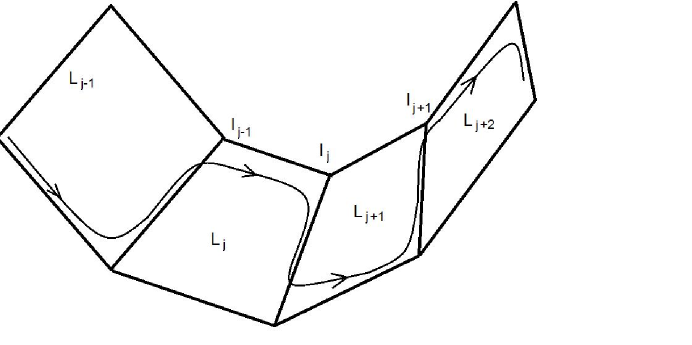
  Figure 1: Planes approximating solutions

• (Integrable dynamics in each plane $L_{j}$)

  Dynamics in each $2$-dimensional plane $L_{j}$ is integrable. Indeed, there are two first integrals $h_{j}$ and $M_{j}$ in involution. By Arnold-Liouville theorem away from degeneracies the $4$-dimensional plane $L_{j}$ is foliated by $2$-dimensional invariant tori with dynamics smoothly conjugated to a constant flow.

  We are interested in two specific periodic orbits: $\theta_{j}$-direction $\{|b_{j}|=1,\ b_{j+1}=0\}$ and $\theta_{j+1}$-direction $\{|b_{j+1}|=1,\ b_{j}=0\}$ and in a family of heteroclinic orbits $\{\gamma_{j}\}$ connecting the former with the later. All these orbits can be found explicitly, but their existence can be predicted having $h_{j}$ and $\mathcal{M}_{j}$ satisfying some properties.

  • Having the mass $\mathcal{M}_{j}=|b_{j}|^{2}+|b_{j+1}|^{2}$ conserved it is natural to expect that the boundary is invariant. The boundary consists of $b_{j}=0$ and $b_{j+1}=0$ (both periodic orbits) and belong to the same $h_{j}$-energy surface.

  • It is a straightforward calculation to check that both orbits are hyperbolic, i.e. of saddle type.

  • Notice that $\{h_{j}=\frac{1}{4},\ \mathcal{M}_{j}=1\}$ is a $2$-dimensional surface with the boundary given by periodic orbits $b_{j}=0$ and $b_{j+1}=0$. Away from these periodic orbits it is a locally analytic surface, i.e. gradients $\nabla h_{j}$ and $\nabla\mathcal{M}_{j}$ are linearly independent.

  • Away from the periodic orbits $b_{j}=0$ and $b_{j+1}=0$ the surface $\{h_{j}=\frac{1}{4},\ \mathcal{M}_{j}=1\}$ consists of stable and unstable $2$-dimensional manifolds. Unless the periodic orbits $b_{j}=0$ and $b_{j+1}=0$ on $\{h_{j}=\frac{1}{4},\ \mathcal{M}_{j}=1\}$ are separated by a degenerate periodic orbit, they have to be connected by these manifolds.

  • Now we verify that there is no such a degenerate periodic orbit. Moreover, we find explicitly the family of connecting heteroclinic orbits. Even though these explicit formulas is not used in our proof.

  Write in polar coordinates $b_{k}=\sqrt{r}_{k}\,e^{i\theta_{k}},\ k=j,j+1$. The mass conservation becomes $\mathcal{M}_{j}(b)=r_{j}+r_{j+1}$, the symplectic form $\Omega=\dfrac{1}{2}dr_{j}\wedge d\theta_{j}$ and the Hamiltonian

  $$h_{j}\left(\sqrt{r_{j}}\ e^{i\theta_{j}},\sqrt{r_{j+1}}\ e^{i\theta_{j+1}}\right)=\dfrac{1}{4}\left[r_{j}^{2}+r_{j+1}^{2}+4r_{j}r_{j+1}\cos 2(\theta_{j}-\theta_{j+1}))\right].$$

  Then the equation of motion are

  $$\dot{\theta}_{j} =r_{j}-2r_{j+1}\cos 2(\theta_{j}-\theta_{j+1})$$

  $$\dot{\theta}_{j+1} =r_{j+1}-2r_{j}\cos 2(\theta_{j}-\theta_{j+1})$$

  $$\dot{r}_{j} =4r_{j}\,r_{j+1}\sin 2(\theta_{j}-\theta_{j+1})$$

  $$\dot{r}_{j+1} =-4r_{j}\,r_{j+1}\sin 2(\theta_{j}-\theta_{j+1}).$$

  For the energy surface $h_{j}=\dfrac{1}{4}$ we have

  • Two families of periodic solutions
    $\{(\theta_{j},\theta_{j+1},r_{j},r_{j+1}):\ r_{j}=0\}$ and $\{(\theta_{j},\theta_{j+1},r_{j},r_{j+1}):\ r_{j+1}=0\}$.

    

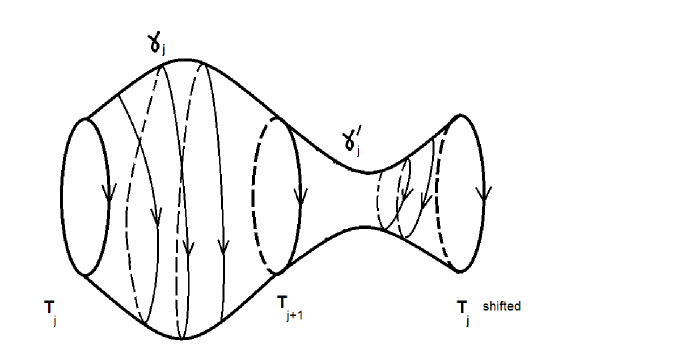
    Figure 2: Heteroclinic orbits

  • Each family has two special solutions: $2(\theta_{j}-\theta_{j+1})$ equals either $\frac{2\pi}{3}$ and $\frac{4\pi}{3}$. Both planes are invariant: $\frac{d}{dt}{(\theta_{j}-\theta_{j+1})}=-(r_{j}+r_{j+1})(1+2\cos 2(\theta_{j}-\theta_{j+1}))=0.$ Denote $\mathbb{T}_{j}=\{2(\theta_{j}-\theta_{j+1})=\frac{2\pi}{3}\ (\text{ mod }2\pi),\ r_{j}=0\}$.

  • On $\mathcal{M}_{j}=1,\ h_{j}=\frac{1}{4},\ \theta_{j}-\theta_{j+1}=\frac{2\pi}{3}$ we have $\dot{r}_{j}=r_{j}r_{j+1}=-\dot{r}_{j+1}$. Thus, there is a heteroclinic orbit $\gamma_{j}$ connecting $\mathbb{T}_{j}$ with the second family $r_{j+1}=0$.

  Now we can be more specific in location of orbits:

  $$\begin{aligned} \textit{ The solutions constructed go from one periodic orbit }\ \mathbb{T}_{2}\textit{ to the next }\ \mathbb{T}_{3}\\ \textit{ along }\gamma_{2},\textit{ then from }\ \mathbb{T}_{3}\textit{ to }\ \mathbb{T}_{4}\ \textit{ along }\gamma_{3}\textit{ and so on for }j=4,\dots,N-2.\end{aligned}$$ (3)

  In a view of the above discussion we have the following description:

  $$\begin{aligned} \leadsto\qquad&\leadsto\ \mathbb{T}_{j}\ \leadsto&\qquad\leadsto\ \gamma_{j}\ \leadsto\qquad\qquad&\qquad\leadsto\ \mathbb{T}_{j+1}\qquad\leadsto\\ &\dot{\theta}_{i}\approx 0,\ |i-j|>1\qquad&\qquad\theta_{j}-\theta_{j+1}\approx\frac{\pi}{3}\qquad&\qquad\dot{\theta}_{i}\approx 0,\ |i-j-1|>1\\ &|b_{i}|\approx 0,\ i\neq j,j+1\qquad&|b_{j}|\leadsto|b_{j+1}|\qquad\quad&\qquad|b_{i}|\approx 0,\ i\neq j+1,j+2.\end{aligned}$$ (4)

• (Local behavior of periodic orbits $\mathbb{T}_{j}$) Due to the above analysis, the periodic orbits $\mathbb{T}_{j}$ viewed in $\mathbb{R}^{2N}$ have at least two expanding and two contracting directions: one pair from $L_{j-1}$-plane and the other from $L_{j}$-pane. Due to symmetry of the restricted systems in $L_{j-1}$-plane and $L_{j}$-plane these periodic orbits have multiple hyperbolic eigenvalues. Multiplicity turns out to be exactly $2$.

• (Resonant normal forms near $\mathbb{T}_{j}$) Presence of resonance complicated analysis and as formulas (4.3) show resonance changes local behavior compare to the linear case. To resolve it we use a beautiful trick of Shilnikov [Šil67] and obtain precise information about local behavior, which is explained in Section 2.2.

• (Connecting heteroclinic orbits) As we showed above there are orbits $\gamma_{j}$ connecting $\mathbb{T}_{j}$ with $\mathbb{T}_{j+1}$ for each $j=3,\dots,n-2$. We need to analyze dynamics near these heteroclinic orbits.

• (Local almost product structure) Once we obtain information about behavior near $\mathbb{T}_{j}$’s and near connecting orbits $\gamma_{j}$, we can describe dynamics of the Toy Model as if it close to the direct product of $(N-3)$ planes $L_{j},\ j=3,\dots,N-1$.

Properties of the Hamiltonian $h(b)$ used in the proof.

As we mentioned in the introduction to this section we do not use a specific form of $h$. Here is the list of properties that we need.

• $h$ has nearest neighbors interaction;

• $h$ has $2$-dimensional (complex) invariant planes intersecting transversally;

• there are two first integrals (coming from two conserved quantities: energy and mass);

• some generic properties of $h$ and $\mathcal{M}$.

2.2 The dynamics close to the periodic orbits: a heuristic model

One of the crucial steps in analyzing the toy model $h(b)$ is the study of the dynamics in a neighborhood of the periodic orbits $\mathbb{T}_{j}$. Namely, we want to analyze how points which lie close their stable invariant manifold evolve under the flow until reaching points close to their unstable one (see Figure 3). As we have explained, these periodic orbits are of mixed type (four eigenvalues are hyperbolic and the rest are elliptic). Since in each plane $L_{j}$ dynamics is the same explained in the previous section, the hyperbolic eigenvalues have multiplicity two and, therefore, are equal to $\lambda,\lambda,-\lambda,-\lambda$ for some $\lambda>0$. Since in this section serves exposition purposes we let $\lambda=1$ and set the elliptic modes to zero.

Essentially the study has three steps:

• Using conservation of $\mathcal{M}$, make a simplectic reduction so the periodic orbit $\mathbb{T}_{j}$ becomes a fixed point.

• Perform a normal form procedure to reduce the size of the higher order non-resonant terms.

• Analyze the dynamics of the new vector field and achieve a cancelation for a local map.

The first step is performed in Section 4.1. It leads to a Hamiltonian of two degrees of freedom of the form

$$H(p,q)=p_{1}q_{1}+p_{2}q_{2}+H_{4}(q,p),$$

where $H_{4}$ is a homogeneous polynomial of degree four. The variables $(p_{1},q_{1})$ correspond to the variable $b_{j-1}$ after diagonalizing the saddle and the variables $(q_{2},p_{2})$ correspond to $b_{j+1}$.

Fix a small $\sigma>0$. To study the local dynamics, it suffices to analyze a map from a section $\Sigma_{-}=\{q_{1}=\sigma,\ |p_{1}|,|q_{2}|,|p_{2}|\ll\sigma\}$, to a section $\Sigma_{+}=\{p_{2}=\sigma,\ |p_{1}|,|q_{1}|,|q_{2}|\ll\sigma\}$ (see Figure 3). Using rescaling assume $\sigma=1$. This can change time by a fixed factor.

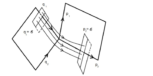
Figure 3: Local map

Since we are in a neighborhood of the origin, one would expect that the dynamics of the system associated to this Hamiltonian is well approximated by its first order, that is, by a linear equation. Then, the solutions are just given by

$$\begin{split}p_{1}(t)&=p_{1}^{0}e^{t},\,\,\,q_{1}(t)=q_{1}^{0}e^{-t}\\ p_{2}(t)&=p_{2}^{0}e^{t},\,\,\,q_{2}(t)=q_{2}^{0}e^{-t}\\ \end{split}$$

and then the local map $\mathcal{B}_{0}$ from $U\subset\Sigma_{-}$ to $\Sigma_{+}$ for this system sends points

$$\left(p_{1}^{0},q_{1}^{0},p_{2}^{0},q_{2}^{0}\right)\sim\left(\delta,1,\sqrt{\delta},\sqrt{\delta}\right)$$

to

$$\mathcal{B}_{0}\left(p_{1}^{0},q_{1}^{0},p_{2}^{0},q_{2}^{0}\right)\sim\left(\sqrt{\delta},\sqrt{\delta},1,\delta\right),$$

where $0<\delta\ll 1$. Moreover, the travel time of orbits by this map is always $T=-\ln\sqrt{\delta}+\mathcal{O}(1)$.

We will see that the image point changes substantially when we add $H_{4}$ to the system, due to both resonant and nonresonant terms. To exemplify this, we consider a simplified model which in fact contains all the difficulties that the true model has,

$$H(p,q)=p_{1}q_{1}+p_{2}q_{2}+q_{1}^{2}p_{2}^{2}+p_{1}^{2}p_{2}^{2}.$$ (5)

Since the term $p_{1}^{2}p_{2}^{2}$ is nonresonant, we first perform one step of normal form $(x,y)=\Psi(p,q)$ (see Section 5 for details). It can be easily seen that the change $\Psi$ is of the form

$$\Psi(p,q)=\left(p_{1},q_{1}+\mathcal{O}(p_{1}p_{2}^{2}),p_{2},q_{2}+\mathcal{O}(p_{1}^{2}p_{2})\right)$$ (6)

and, therefore, keeps the size of initial points of the form

$$\left(p_{1}^{0},q_{1}^{0},p_{2}^{0},q_{2}^{0}\right)\sim\left(\delta,1,\sqrt{\delta},\sqrt{\delta}\right).$$

That is, $(x^{0},y^{0})=\Psi(p^{0},q^{0})$ satisfies

$$\left(x_{1}^{0},y_{1}^{0},x_{2}^{0},y_{2}^{0}\right)\sim\left(\delta,1,\sqrt{\delta},\sqrt{\delta}\right).$$

The change to normal form leads to a Hamiltonian system of the form

$$H^{\prime}(x,y)=x_{1}q_{1}+x_{2}y_{2}+y_{1}^{2}x_{2}^{2}+\text{higher order terms}.$$

Drop the higher order terms. Then, the solutions of the system associated to this Hamiltonian can be computed explicitly and are given by

$$\begin{split}x_{1}&=x_{1}^{0}e^{t}+2y_{1}^{0}(x_{2}^{0})^{2}te^{t}=\left(x_{1}^{0}+2y_{1}^{0}(x_{2}^{0})^{2}t\right)e^{t}\\ y_{1}&=y_{1}^{0}e^{-t}\\ x_{2}&=x_{2}^{0}e^{t}\\ y_{2}&=y_{2}^{0}e^{-t}-2(y_{1}^{0})^{2}x_{2}^{0}te^{t}.\\ \end{split}$$

Thus, since the travel time is $t=-\ln\,\sqrt{\delta}+\mathcal{O}(1)$, it is clear that the nonlinear terms are bigger than the linear ones, leading to an image point of the form

$$\left(x_{1}^{f},y_{1}^{f},x_{2}^{f},y_{2}^{f}\right)\sim\left(\sqrt{\delta}\ln(1/\delta),\sqrt{\delta},1,\delta\ln(1/\delta)\right).$$

Using (6), in the original variables the image point of the map $\mathcal{B}_{1}$ associated to Hamiltonian $H$ is of the form

$$\mathcal{B}_{1}\left(p_{1}^{0},q_{1}^{0},p_{2}^{0},q_{2}^{0}\right)\sim\left(\sqrt{\delta}\ln(1/\delta),\sqrt{\delta},1,\delta\ln^{2}(1/\delta)\right).$$

We want to emphasize that the presence of these logarithmic terms is a serious problem we need to deal with. Recall that we need to travel through $N-3$ saddles ($\mathbb{T}_{3}\leadsto\mathbb{T}_{4}\leadsto\ldots\leadsto\mathbb{T}_{N-1}$). Roughly speaking, this implies that we need to compose $N-4$ local maps. Thanks to the symmetries, at each saddle we can consider a system of coordinates such that the dynamics is essentially given by a Hamiltonian of the form (5). Moreover, since at each local map we gain some logarithms, the initial points of the local map associated to the $j$ saddle are of the form

$$\left(p_{1}^{0},q_{1}^{0},p_{2}^{0},q_{2}^{0}\right)\sim\left(\delta\ln^{2^{j-1}}(1/\delta),1,\sqrt{\delta},\sqrt{\delta}\right),$$

which, thanks to (6), in the normal form variables satisfy

$$\left(x_{1}^{0},y_{1}^{0},x_{2}^{0},y_{2}^{0}\right)\sim\left(\delta\ln^{2^{j-1}}(1/\delta),1,\sqrt{\delta},\sqrt{\delta}\right).$$

Then, proceeding as before, these points are mapped to points of the form

$$\left(x_{1}^{f},y_{1}^{f},x_{2}^{f},y_{2}^{f}\right)\sim\left(\sqrt{\delta}\ln^{2^{j-1}}(1/\delta),\delta^{1/2},1,\delta\ln(1/\delta)\right)$$

which in the original variables read

$$\mathcal{B}_{1}\left(p_{1}^{0},q_{1}^{0},p_{2}^{0},q_{2}^{0}\right)\sim\left(\sqrt{\delta}\ln^{2^{j-1}}(1/\delta),\sqrt{\delta},1,\delta\ln^{2^{j}}(1/\delta)\right).$$

That is, the amount of logarithms doubles at each step and thus grows exponentially. This accumulation of logarithmic terms leads to very bad estimates. Indeed, to keep track of the orbit after $N-4$ local maps, we would need that

$$\delta\ln^{2^{N-4}}(1/\delta)\ll 1.$$

Therefore, we would need to choose $\delta$ extremely small with respect to $N$.

For example, if $\delta\gtrsim C^{-\mathcal{K}^{2a}}\sim C^{-\,2^{aN}}$ for some $C>0$ independent of $N$, then the above expression gives

$$C^{-\,2^{aN}}(2^{aN}\,\ln C)^{2^{N-4}}\gg 1\text{ for }a\leq 1.$$

In this case, the constant $\lambda$ appearing in Theorem 4 would need to satisfy $\lambda\sim\delta^{-b}$ for some $b>0$ and independent of $N$. As a result, Theorem 3 gives a diffusion time $T\sim\lambda^{2}\mathbb{K}\gamma N\ln 1/\delta\gtrsim C^{\mathcal{K}^{2}}$ (see formula (22)). Thus, choosing such a small $\delta$ would lead to very bad estimates for the diffusion time of Sobolev norms as we pointed out in Remark 1.4.

To overcome this problem, we modify slightly the initial conditions. Notice that if we choose $x_{1}^{0}$ such that

$$x_{1}^{0}-2y_{1}^{0}(x_{2}^{0})^{2}\ln\,\sqrt{\delta}=0,$$

we obtain that at the end $x_{1}^{f}\sim\sqrt{\delta}$ and thus we avoid the logarithmic term. This cancelation will be crucial in our proof. If we restrict $x_{1}^{0}$ to this set, we are taking $x_{1}^{0}\sim\delta\ln(1/\delta)$ and therefore we will be sending points

$$\left(x_{1}^{0},y_{1}^{0},x_{2}^{0},y_{2}^{0}\right)\sim\left(\delta\ln(1/\delta),1,\sqrt{\delta},\sqrt{\delta}\right),$$

to points

$$\left(x_{1}^{f},y_{1}^{f},x_{2}^{f},y_{2}^{f}\right)\sim\left(\sqrt{\delta},\sqrt{\delta},1,\delta\ln(1/\delta)\right).$$

The map will keep the same form expressed in the original variables, and, therefore, we will avoid having increasing separation from the invariant manifolds.

2.3 Outline of the Proof

• Find symplectic coordinates near the origin in $\ell^{1}$, where the original Hamiltonian $\mathcal{H}$ simplifies (see Theorem 2). Namely, $\mathcal{H}\circ\Gamma=\mathcal{D}+\widetilde{\mathcal{G}}+\mathcal{R}$, where $\mathcal{D}$ is a quadratic Hamiltonian, $\widetilde{\mathcal{G}}$ is of degree four and only contains resonant terms, and $\mathcal{R}$ is smaller.

• Dynamics of $\mathcal{D}+\widetilde{\mathcal{G}}$ has invariant finite-dimensional subspaces, which give rise to a simpler (no simple!) finite-dimensional Hamiltonian $h(b)$ given by (19). In terminology of [CKS⁺10] this Hamiltonian defines the Toy Model. In Theorem 3 we obtain orbits of the toy model which have transfer of energy.

• We show that are solutions of the system associated to $\mathcal{H}$ which are close to those of the toy model for long enough time (Theorem 4). These orbits undergo the wanted growth of the Sobolev norm.

• The proof of Theorem 3 occupies most of the paper. Theorems 2 and 4 are deferred to Appendices A and B respectively. Now we describe the plan of the proof of Theorem 3.

• Following [CKS⁺10] we detect a collection of periodic orbits $\{\mathbb{T}_{j}\}_{j=1}^{N-1}$ of $h(b)$, defined in (32), and heteroclinic orbits $\{\gamma_{j}\}_{j=1}^{N-2}$ connecting them (see (33)).

  The whole proof consists in a careful analysis of dynamics near the union of these periodic orbits and their connecting orbits. Our analysis naturally splits into

  • local dynamics near periodic orbits $\{\mathbb{T}_{j}\}_{j=1}^{N-1}$ and

  • global dynamics near heteroclinic orbits $\{\gamma_{j}\}_{j=1}^{N-2}$.

• More formally, Theorem 3 follows from Theorem 5. The latter Theorem in turn follows from Lemmas 4.7 and 4.8.

• The Local Lemma 4.7 provides refined information about local behavior near periodic orbits $\{\mathbb{T}_{j}\}_{j}$ with quantitative estimates.

• Global Lemma 4.8 provides refined information about local behavior near heteroclinic orbits from (33) with quantitative estimates.

• The proof of Local Lemma 4.7 consists of several steps. As we have explained in Section 2.1, the periodic orbits $\{\mathbb{T}_{j}\}_{j}$ have mixed type. Namely, in some directions the local behavior is hyperbolic, while in others it is elliptic. It turns out that the closer orbits under investigation pass to the periodic orbits $\{\mathbb{T}_{j}\}_{j}$, the more decoupled (direct product-like) behavior they have.

• In Section 5 we set all the elliptic variables zero and study the ($4$-dimensional) hyperbolic Toy Model.

• In Section 6 we use these results to deal with the full hyperbolic-elliptic system and prove Lemma 4.7.

• In Section 7 we prove Global Lemma 4.8. As we pointed out, this implies Theorem 5, which in turn, implies Theorem 3.

• Combining this result with Theorem 2, proved in Appendix A, and Theorem 4 proved in Appendix B, we complete the proof of the main result (Theorem 1).

We summarize this in the following diagram:

$$\begin{aligned} \qquad\boxed{\text{ Theorem \ref{thm:main} }}\qquad\qquad\qquad\qquad\\ \Uparrow\quad\qquad\qquad\qquad\qquad\qquad\\ \overbrace{\boxed{\text{ Theorem \ref{thm:NormalForm}}}+\quad\underbrace{\boxed{\text{ Theorem \ref{thm:ToyModelOrbit} }}}\quad+\ \boxed{\text{ Theorem \ref{thm:Approximation} }}}\ \\ \Uparrow\quad\qquad\qquad\qquad\qquad\qquad\\ \qquad\boxed{\text{ Theorem \ref{theorem:iterative} }}\qquad\qquad\qquad\qquad\\ \Uparrow\quad\qquad\qquad\qquad\qquad\qquad\\ \overbrace{\boxed{\text{ Local Lemma \ref{lemma:iterative:saddle}}}\ \ +\ \boxed{\text{ Global Lemma \ref{lemma:iterative:hetero} }}}\qquad\end{aligned}$$ (7)

2.4 Major ingredients of the proof

We summarize here the new set of tools that we apply to the problem compared to [CKS⁺10].

• In Theorem 2, we use a standard normal form (e.g. see [KP96]).

• Theorem 3 requires several new ideas:

  • Finitely smooth resonant normal form for hyperbolic saddles [BK94].

  • Shilnikov boundary value problem [Šil67] to study the local behavior close to the periodic orbits $\mathbb{T}_{j}$.

  • As we explained for the model case in Section 2.2, to control the dynamics of the toy model we need a peculiar cancellation (see Section 5).

  • To have cancellations at each stage, we need to establish local product structure for the orbits we are interested in (see Definition 4.3).

• Due to the good control of the solutions of the toy model, we are able to approximate the solutions of the original systems with the ones of the toy model for longer time compared with [CKS⁺10] (see Theorem 4). To achieve this, we also modify the set $\Lambda$ (see condition $6_{\Lambda}$). This modification allows to slow down spreading outside $\Lambda$.

3 The three key theorems

We start the proof analyzing the infinite system of equations which describe the behavior of Fourier coefficients. Namely, consider the Fourier series of $u$,

$$u(t,x)=\sum_{n\in\mathbb{Z}^{2}}a_{n}(t)e^{inx},\qquad a_{n}(t):=\hat{u}(t,n).$$

Therefore, the equation (1) becomes an infinite system of equations for $\{a_{n}\}_{n\in\mathbb{Z}^{2}}$, which are given by

$$-i\dot{a}_{n}=|n|^{2}a_{n}+\sum_{\begin{subarray}{c}n_{1},n_{2},n_{3}\in\mathbb{Z}^{2}\\ n_{1}-n_{2}+n_{3}=n\end{subarray}}a_{n_{1}}\overline{a_{n_{2}}}a_{n_{3}}.$$ (8)

Note that this equation is Hamiltonian. Indeed, it can be written as

$$\dot{a}_{n}=2i\partial_{\ \overline{a_{n}}}\ \mathcal{H}(a,\overline{a}),$$

where

$$\mathcal{H}(a,\overline{a})=\mathcal{D}(a,\overline{a})+\mathcal{G}(a,\overline{a})$$ (9)

with

$$\mathcal{D}(a,\overline{a}) =\frac{1}{2}\sum_{n\in\mathbb{Z}^{2}}|n|^{2}|a_{n}|^{2}$$

$$\mathcal{G}(a,\overline{a}) =\frac{1}{4}\sum_{\begin{subarray}{c}n_{1},n_{2},n_{3},n_{4}\in\mathbb{Z}^{2}\\ n_{1}-n_{2}+n_{3}=n_{4}\end{subarray}}a_{n_{1}}\overline{a_{n_{2}}}a_{n_{3}}\overline{a_{n_{4}}}.$$

We will study equation (8) in a family of Banach spaces: all $H^{s}$-Sobolev spaces with $s>1$ as well as in the $\ell^{1}$-space. The $\ell^{1}$ space is defined as

$$\ell^{1}=\left\{a:\mathbb{Z}^{2}\rightarrow\mathbb{C}:\|a\|_{\ell^{1}}=\sum_{n\in\mathbb{Z}^{2}}|a_{n}|<\infty\right\}.$$

Note that, $\ell^{1}$ is a Banach algebra with respect to the convolution product. Namely, if $a,b\in\ell^{1}$ its convolution product $a\ast b$, which is defined by

$$(a\ast b)_{n}=\sum_{n_{1}+n_{2}=n}a_{n_{1}}b_{n_{2}}$$

satisfies

$$\|a\ast b\|_{\ell^{1}}\leq\|a\|_{\ell^{1}}\|b\|_{\ell^{1}}.$$

Finally, let us point out that the $L^{2}$-norm conservation of (1), becomes now conservation of the $\ell^{2}$-norm of $a$, defined as above. Namely, we have that $\|a(t)\|_{\ell^{2}}=\|a(0)\|_{\ell^{2}}$ for all $t\in\mathbb{R}$.

We want to study the evolution of certain solutions of equation (8), which will be small in the $\ell^{1}$ norm. Now we make an outline of the proof.

The first step is to find out which terms make the biggest contribution to this evolution. To this end, we perform one step of normal form and bound the remainder in the $\ell^{1}$-norm.

Theorem 2.

For the Hamiltonian $\mathcal{H}$ in (9) there exists a symplectic change of coordinates $a=\Gamma(\alpha)$ in a neighborhood of $0$ in $\ell^{1}$ which takes it into its Birkhoff normal form up to order four, that is,

$$\mathcal{H}\circ\Gamma=\mathcal{D}+\widetilde{\mathcal{G}}+\mathcal{R},$$

where $\widetilde{\mathcal{G}}$ only contains resonant terms, namely

$$\widetilde{\mathcal{G}}(\alpha,\overline{\alpha})=\frac{1}{4}\sum_{\begin{subarray}{c}n_{1},n_{2},n_{3},n_{4}\in\mathbb{Z}^{2}\\ n_{1}-n_{2}+n_{3}=n_{4}\\ |n_{1}|^{2}-|n_{2}|^{2}+|n_{3}|^{2}=|n_{4}|^{2}\end{subarray}}\alpha_{n_{1}}\overline{\alpha_{n_{2}}}\alpha_{n_{3}}\overline{\alpha_{n_{4}}}$$

and $X_{\mathcal{R}}$, the vector field associated to the Hamiltonian $\mathcal{R}$, satisfies

$$\|\mathcal{X}_{\mathcal{R}}\|_{\ell^{1}}\leq\mathcal{O}\left(\|\alpha\|_{\ell^{1}}^{5}\right).$$

Moreover, the change $\Gamma$ satisfies

$$\left\|\Gamma-\mathrm{Id}\right\|_{\ell^{1}}\leq\mathcal{O}\left(\|\alpha\|_{\ell^{1}}^{3}\right).$$

The proof of this theorem is postponed to Appendix A.

Once we perform one step of normal form, we have a new vector field

$$-i\dot{\alpha}_{n}=|n|^{2}\alpha_{n}+\sum_{(n_{1},n_{2},n_{3})\in\mathcal{A}_{0}(n)}\alpha_{n_{1}}\overline{\alpha_{n_{2}}}\alpha_{n_{3}}+\partial_{\overline{\alpha}_{n}}\mathcal{R},$$ (10)

where

$$\begin{split}\mathcal{A}_{0}(n)=\Big{\{}&(n_{1},n_{2},n_{3})\in\left(\mathbb{Z}^{2}\right)^{3}:\,n_{1}-n_{2}+n_{3}=n,\\ &|n_{1}|^{2}-|n_{2}|^{2}+|n_{3}|^{2}=|n|^{2}\Big{\}}.\end{split}$$ (11)

As a first step, we focus our attention to the degree 4 truncation of it, which will give the main contribution to the dynamics. Namely, we consider the Hamiltonian

$$\mathcal{H}^{\prime}=\mathcal{D}+\widetilde{\mathcal{G}},$$

which has associated equations

$$-i\dot{\alpha}_{n}=|n|^{2}\alpha_{n}+\sum_{(n_{1},n_{2},n_{3})\in\mathcal{A}_{0}(n)}\alpha_{n_{1}}\overline{\alpha_{n_{2}}}\alpha_{n_{3}}.$$ (12)

Note that the $\ell^{2}$-norm of $\alpha$ is a first integral of this system as well as for (8) and (10). Namely,

$$\|\alpha(t)\|_{\ell^{2}}=\|\alpha(0)\|_{\ell^{2}}\,\,\,\text{for all }t\in\mathbb{R}.$$

Then, to study the dynamics of $\alpha$ close to the origin (in the $\ell^{1}$-norm) we remove its linear terms using the variation of constants formula. Moreover, following [CKS⁺10], we also remove certain cubic terms using the gauge freedom of equation (1). To this end, we make the change of coordinates

$$\alpha_{n}=\beta_{n}e^{i\left(G+|n|^{2}\right)t},$$ (13)

where $G>0$ is a constant to be determined. The equations for $\beta$ read

$$-i\dot{\beta}_{n}=G\beta_{n}+\sum_{(n_{1},n_{2},n_{3})\in\mathcal{A}_{0}(n)}\beta_{n_{1}}\overline{\beta_{n_{2}}}\beta_{n_{3}}.$$

Choosing $G$ properly we can remove certain terms in the sum. Indeed, we split the sum as

$$\sum_{(n_{1},n_{2},n_{3})\in\mathcal{A}_{0}(n)}=\sum_{\begin{subarray}{c}(n_{1},n_{2},n_{3})\in\mathcal{A}_{0}(n)\\ n_{1},n_{3}\neq n\end{subarray}}+\sum_{\begin{subarray}{c}(n_{1},n_{2},n_{3})\in\mathcal{A}_{0}(n)\\ n_{1}=n\end{subarray}}+\sum_{\begin{subarray}{c}(n_{1},n_{2},n_{3})\in\mathcal{A}_{0}(n)\\ n_{3}=n\end{subarray}}-\sum_{\begin{subarray}{c}(n_{1},n_{2},n_{3})\in\mathcal{A}_{0}(n)\\ n_{1}=n_{3}=n\end{subarray}}$$

The last sum is just one term, which is given by $-\beta_{n}|\beta_{n}|^{2}$. The second and third sums, are in fact single sums and each of them is given by

$$\beta_{n}\sum_{k\in\mathbb{Z}^{2}}|\beta_{k}|^{2}=\beta_{n}\|\beta\|_{\ell^{2}}^{2}.$$

Recall that both (12) and (13) preserve the $\ell^{2}$-norm. Therefore, taking $G=-2\|\alpha\|^{2}_{\ell^{2}}=-2\|\beta\|^{2}_{\ell^{2}}$, we can remove these two terms. Thus, with this choice, we obtain the equation for $\beta$, which reads

$$-i\dot{\beta}_{n}=-\beta_{n}|\beta_{n}|^{2}+\sum_{n_{1},n_{2},n_{3}\in\mathcal{A}(n)}\beta_{n_{1}}\overline{\beta_{n_{2}}}\beta_{n_{3}}$$ (14)

where

$$\begin{split}\mathcal{A}(n)=\Big{\{}&(n_{1},n_{2},n_{3})\in\left(\mathbb{Z}^{2}\right)^{3}:\,n_{1}-n_{2}+n_{3}=n\\ &|n_{1}|^{2}-|n_{2}|^{2}+|n_{3}|^{2}=|n|^{2},n_{1}\neq n,n_{3}\neq n\Big{\}}.\end{split}$$

We define also the set of all resonant frequencies as

$$\mathcal{A}=\Big{\{}(n_{1},n_{2},n_{3},n_{4})\in\left(\mathbb{Z}^{2}\right)^{4}:\,(n_{1},n_{2},n_{3})\in\mathcal{A}(n_{4})\Big{\}}.$$

Note that if $(n_{1},n_{2},n_{3},n_{4})\in\mathcal{A}$, then the four points form a rectangle in $\mathbb{Z}^{2}$.

We reduce this system to a finite-dimensional one, which corresponds to an invariant finite-dimensional plane. To this end, we consider a set $\Lambda\subset\mathbb{Z}^{2}$ such that the corresponding harmonics do not interact to the harmonics outside of $\Lambda$. Moreover, we obtain a set $\Lambda$ such that the harmonics in $\Lambda$ interact in a very particular way. This set was constructed in [CKS⁺10]. We explain now its construction and impose an additional condition on $\Lambda$ from [CKS⁺10].

Fix $N\gg 1$. Following [CKS⁺10] we define a set $\Lambda\subset\mathbb{Z}^{2}$ consisting of $N$ pairwise disjoint generations:

$$\Lambda=\Lambda_{1}\cup\ldots\cup\Lambda_{N}.$$

Define a nuclear family to be a rectangle $(n_{1},n_{2},n_{3},n_{4})\in\mathcal{A}$, such that $n_{1}$ and $n_{3}$ (known as the parents) belong to a generation $\Lambda_{j}$ and $n_{2}$ and $n_{4}$ (known as the children) live in the next generation $\Lambda_{j+1}$. Note that if $(n_{1},n_{2},n_{3},n_{4})$ is a nuclear family, then so are $(n_{1},n_{4},n_{3},n_{2})$, $(n_{3},n_{2},n_{1},n_{4})$ and $(n_{3},n_{4},n_{1},n_{2})$. These families are called trivial permutations of the family $(n_{1},n_{2},n_{3},n_{4})$.

The conditions to impose to the set $\Lambda$ are

$1_{\Lambda}$ Closure

If $n_{1},n_{2},n_{3}\in\Lambda$ and $(n_{1},n_{2},n_{3})\in\mathcal{A}(n)$, then $n\in\Lambda$. In other words, if three vertices of a rectangle are in $\Lambda$ so is the last fourth one.

$2_{\Lambda}$ Existence and uniqueness of spouse and children

For any $1\leq j<N$ and any $n_{1}\in\Lambda_{j}$, there exists a unique nuclear family $(n_{1},n_{2},n_{3},n_{4})$ (up to trivial permutations) such that $n_{1}$ is a parent of this family. In particular, each $n_{1}\in\Lambda_{j}$ has a unique spouse $n_{3}\in\Lambda_{j}$ and has two unique children $n_{2},n_{4}\in\Lambda_{j+1}$ (up to permutation).

$3_{\Lambda}$ Existence and uniqueness of sibling and parents

For any $1\leq j<N$ and any $n_{2}\in\Lambda_{j+1}$, there exists a unique nuclear family $(n_{1},n_{2},n_{3},n_{4})$ (up to trivial permutations) such that $n_{2}$ is a child of this family. In particular each $n_{2}\in\Lambda_{j+1}$ has a unique sibling $n_{4}\in\Lambda_{j+1}$ and two unique parents $n_{1},n_{3}\in\Lambda_{j}$ (up to permutation).

$4_{\Lambda}$ Nondegeneracy

The sibling of a frequency $n$ never equal to its spouse.

$5_{\Lambda}$ Faithfulness

Apart from the nuclear families, $\Lambda$ does not contain any other rectangle.

These are the conditions imposed on $\Lambda$ in [CKS⁺10]. We will impose an additional condition:

$6_{\Lambda}$ No spreading condition

Let us consider $n\not\in\Lambda$. Then, $n$ is vertex of at most two rectangles having two vertices in $\Lambda$ and two vertices out of $\Lambda$.

Proposition 3.1.

Let $\mathcal{K}\gg 1$. Then, there exists $N\gg 1$ large and a set $\Lambda\subset\mathbb{Z}^{2}$, with

$$\Lambda=\Lambda_{1}\cup\ldots\cup\Lambda_{N},$$

which satisfies conditions $1_{\Lambda}$ – $6_{\Lambda}$ and also

$$\frac{\sum_{n\in\Lambda_{N-1}}|n|^{2s}}{\sum_{n\in\Lambda_{3}}|n|^{2s}}\geq\dfrac{1}{2}2^{(s-1)(N-4)}\geq\mathcal{K}^{2}.$$ (15)

Moreover, given any $R>0$ (which may depend on $\mathcal{K}$), we can ensure that each generation $\Lambda_{j}$ has $2^{N-1}$ disjoint frequencies $n$ satisfying $|n|\geq R$.

The proof of Proposition 2.1 from [CKS⁺10] applies. We prove a quantitative version of this proposition in Appendix C.

We use the set $\Lambda$ to obtain a finite dimensional dynamical system (of high dimension) approximating (14). To this end, let us first note that, by Property $1_{\Lambda}$, the manifold

$$M=\left\{\beta\in\mathbb{C}^{\mathbb{Z}^{2}}:\beta_{n}=0\,\,\text{for all }n\not\in\Lambda\right\}$$

is invariant by the flow associated to (14) and is finite dimensional. Indeed, by Proposition 3.1 its dimension is $N2^{N-1}$. Equation (14) restricted to $M$ reads as follows. For each $n\in\Lambda$ we have

$$-i\dot{\beta}_{n}=-\beta_{n}|\beta_{n}|^{2}+2\beta_{n_{\mathrm{child}_{1}}}\beta_{n_{\mathrm{child}_{2}}}\overline{\beta_{n_{\mathrm{spouse}}}}+2\beta_{n_{\mathrm{parent}_{1}}}\beta_{n_{\mathrm{parent}_{2}}}\overline{\beta_{n_{\mathrm{sibling}}}}$$ (16)

Indeed, presence of parents, children, and the sibling are guaranteed by $2_{\Lambda}$ and $3_{\Lambda}$. Note, that in the first and last generations, the parents and children are set to zero respectively. In fact, $M$ has a submanifold of considerably lower dimension which is also invariant.

Corollary 3.2.

(cf. [CKS⁺10]) Consider the subspace

$$\widetilde{M}=\left\{\beta\in M:\beta_{n_{1}}=\beta_{n_{2}}\,\,\text{for all }n_{1},n_{2}\in\Lambda_{j}\,\,\text{for some }j\right\},$$

where all the members of a generation take the same value. Then, $\widetilde{M}$ is invariant under the flow associated to (16).

The dimension of $\widetilde{M}$ is equal to the number of generations, namely $N$. To define equation (16) restricted to $\widetilde{M}$, let us define

$$b_{j}=\beta_{n}\,\,\,\text{ for any }n\in\Lambda_{j}.$$ (17)

Then, (16) restricted to $\widetilde{M}$ becomes

$$\dot{b}_{j}=-ib_{j}^{2}\overline{b}_{j}+2i\overline{b}_{j}\left(b_{j-1}^{2}+b_{j+1}^{2}\right),\,\,j=0,\ldots N,$$ (18)

which is a Hamiltonian system with respect to the Hamiltonian

$$h(b):=\frac{1}{4}\sum_{j}|b_{j}|^{4}-\frac{1}{2}\sum_{j}\left(\overline{b}_{j}^{2}b_{j-1}^{2}+b_{j}^{2}\overline{b}_{j-1}^{2}\right)$$ (19)

and the symplectic form $\Omega=\frac{i}{2}db_{j}\wedge d\overline{b}_{j}$.

Theorem 3.

Fix a large $\gamma\gg 1$. Then for any large enough $N$ and $\delta=e^{-\gamma N}$, there exists an orbit of system (18), $\nu>0$ and $T_{0}>0$ such that

$$\begin{split}|b_{3}(0)|&>1-\delta^{\nu}\\ |b_{j}(0)|&<\delta^{\nu}\qquad\text{ for }j\neq 3\end{split}\qquad\text{ and }\qquad\begin{split}|b_{N-1}(T_{0})|&>1-\delta^{\nu}\\ |b_{j}(T_{0})|&<\delta^{\nu}\qquad\text{ for }j\neq N-1.\end{split}$$

Moreover, there exists a constant $\mathbb{K}>0$ independent of $N$ such that $T_{0}$ satisfies

$$0<T_{0}<\mathbb{K}N\ln\left(\frac{1}{\delta}\right)=\mathbb{K}\,\gamma\,N^{2}.$$ (20)

Remark 3.3.

An analog of this proposition also holds for some smaller $\delta$, e.g. $\delta=C^{-\mathcal{K}^{2}}$. This is related to Remark 1.4 about time of diffusion without cancelations.

Using (17), Theorem 3 gives an orbit for equation (14). Moreover, both equations (14) and (18) are invariant under certain rescaling. Indeed if $b(t)$ is a solution of (18),

$$b^{\lambda}(t)=\lambda^{-1}b\left(\lambda^{-2}t\right)$$ (21)

is a solution of the same equation. By Theorem 3 duration of this solution in time is

$$T=\lambda^{2}T_{0}\leq\lambda^{2}\,\mathbb{K}\,\gamma\,N^{2},$$ (22)

where $T_{0}$ is the time obtained in Theorem 3, which satisfies (20).

We will see that, modulo a rotation of the modes (see (13)), there is a solution of equation (10) which is close to the orbit $\beta^{\lambda}$ of (14) defined as

$$\begin{split}\beta^{\lambda}_{n}(t)&=\lambda^{-1}b_{j}\left(\lambda^{-2}t\right)\,\,\,\text{ for each }\ n\in\Lambda_{j}\\ \beta^{\lambda}_{n}(t)&=0\,\,\,\text{ for each }\ n\not\in\Lambda.\end{split}$$ (23)

To have the original system being well approximated by the truncated system, we need that $\lambda$ is large enough. Then the cubic terms in (10) dominate over the quintic ones. Nevertheless, the bigger $\lambda$ is, the slower the instability time by (22). Thus, we look for the smallest $\lambda$ (with respect to $N$) for which the following approximation theorem applies.

Theorem 4.

Let $\alpha(t)=\{\alpha_{n}(t)\}_{n\in\mathbb{Z}^{2}}$ be the solution of (10), $\beta^{\lambda}(t)=\{\beta^{\lambda}_{n}(t)\}_{n\in\mathbb{Z}^{2}}$ be the solution of (14) given by (23) and $T$ be the time defined in (22). Suppose $\mathrm{supp}\,\alpha(0)\subset\Lambda$ and $\alpha(0)=\beta^{\lambda}(0)$. Then, there exist a constant $\kappa>0$ independent of $N$ and $\gamma$ such that, for

$$\lambda=e^{\kappa\gamma N},$$ (24)

and $0<t<T$ we have

$$\sum_{n\in\mathbb{Z}^{2}}\left|\alpha_{n}(t)-e^{i(G+|n|^{2})t}\beta^{\lambda}_{n}(t)\right|\leq\lambda^{-2},$$ (25)

where $G=-2\|\alpha(0)\|_{\ell^{2}}^{2}$.

Using the three key theorems: Theorems 2, 3 and 4 we complete the proof of Theorem 1.

Proof of Theorem 1.

Using the change of variables $\Gamma$ obtained in Theorem 2, from the solution $\alpha$ obtained in Theorem 4 we define $a=\Gamma(\alpha)$, which is a solution of system (8). We show that this orbit has the properties stated in Theorem 1.

To compute the growth of Sobolev norm of this orbit $a$, we use the notation

$$S_{j}=\sum_{n\in\Lambda_{j}}|n|^{2s}\text{ for }j=1,\dots,N-1.$$ (26)

To estimate the mass of our solution recall that $2^{N-1}=\sum_{n\in\Lambda_{j}}1=|\Lambda_{j}|$. We want to prove that

$$\frac{\|a(T)\|_{H^{s}}}{\|a(0)\|_{H^{s}}}\gtrsim\mathcal{K}$$

and estimate the mass $\|a(0)\|_{L^{2}}$ of the solution. To this end, we start by bounding $\|a(T)\|_{H^{s}}$ in terms of $S_{N-1}$. Since

$$\left\|a(T)\right\|^{2}_{H^{s}}\geq\sum_{n\in\Lambda_{N-1}}|n|^{2s}\left|a_{n}(T)\right|^{2}\geq S_{N-1}\inf_{n\in\Lambda_{N-1}}\left|a_{n}(T)\right|^{2},$$

it is enough to obtain a lower bound for $\left|a_{n}(T)\right|$ with $n\in\Lambda_{N-1}$. Using the results of Theorems 2 and 4, we obtain

$$\begin{split}\left|a_{n}(T)\right|\geq&\left|\alpha_{n}(T)\right|-\left|\Gamma_{n}(\alpha)(T)-\alpha_{n}(T)\right|\\ \geq&\left|\beta^{\lambda}_{n}(T)e^{i\left(|n|^{2}+G\right)T}\right|-\left|\alpha_{n}(T)-\beta^{\lambda}_{n}(T)e^{i\left(|n|^{2}+G\right)T}\right|\\ &-\left|\Gamma_{n}(\alpha)(T)-\alpha_{n}(T)\right|.\end{split}$$ (27)

We need to obtain a lower bound for the first term of the right hand side and upper bounds for the second and third ones. Indeed, using the definition of $\beta^{\lambda}$ in (23) and the results in Theorem 3 we have that for $n\in\Lambda_{N-1}$,

$$\left|\beta_{n}^{\lambda}(T)\right|^{2}=\lambda^{-2}\left|b_{N-1}(T_{0})\right|^{2}\geq\frac{3}{4}\lambda^{-2},$$

(the relation between $T$ and $T_{0}$ is established in (22)).

For the second term in the right hand side of (27), it is enough to use Theorem 4 to obtain,

$$\left|\alpha_{n}(T)-\beta^{\lambda}_{n}(T)e^{i\left(|n|^{2}+G\right)T}\right|^{2}\leq\left(\sum_{n\in\mathbb{Z}^{2}}\left|\alpha_{n}(T)-\beta^{\lambda}_{n}(T)e^{i\left(|n|^{2}+G\right)T}\right|\right)^{2}\leq\frac{\lambda^{-2}}{8}.$$

For the lower bound of the third term, we use the bound for $\Gamma-\mathrm{Id}$ given in Theorem 2. Then,

$$\left|\Gamma_{n}(\alpha)(T)-\alpha_{n}(T)\right|^{2}\leq\|\Gamma(\alpha)-\alpha\|_{\ell^{1}}^{2}\leq\frac{\lambda^{-2}}{8}.$$

Thus, we can conclude that

$$\left\|\alpha(T)\right\|^{2}_{H^{s}}\geq\frac{\lambda^{-2}}{2}S_{N-1}.$$ (28)

Now we prove that

$$\left\|a(0)\right\|^{2}_{H^{s}}\lesssim\lambda^{-2}S_{3}\qquad\text{ and }\qquad\left\|a(0)\right\|^{2}_{L^{2}}\lesssim\lambda^{-2}\,2^{N}.$$ (29)

By the definition of $\lambda$ in (24), the second inequality implies that the mass of $a(0)$ is small. On the contrary, the first inequality does not imply that the $H^{s}$-norm of $a(0)$ is small. As a matter of fact $S_{3}$ is large.

To prove the first inequality of (29), let us point out that

$$\left\|a(0)\right\|^{2}_{H^{s}}\leq\sum_{n\in\mathbb{Z}^{2}}|n|^{2s}\left|\alpha_{n}(0)+\left(\Gamma_{n}(\alpha(0)-\alpha_{n}(0)\right)\right|^{2}.$$

We first bound $\left\|\alpha(0)\right\|^{2}_{H^{s}}$. To this end, let us recall that $\mathrm{supp}\ \alpha=\Lambda$. Then,

$$\left\|\alpha(0)\right\|^{2}_{H^{s}}=\sum_{n\in\Lambda}|n|^{2s}\left|\alpha_{n}(0)\right|^{2}.$$

Using Theorem 4, we have that

$$\left\|\alpha(0)\right\|^{2}_{H^{s}}\leq\sum_{n\in\Lambda}|n|^{2s}\left(\left|\beta^{\lambda}_{n}(0)\right|+\left|\beta^{\lambda}_{n}(0)-\alpha_{n}(0)\right|\right)^{2}.$$ (30)

Recalling the definition of $\beta^{\lambda}$ in (23) and the results in Theorem 3,

$$\begin{split}\sum_{n\in\Lambda}|n|^{2s}\left|\beta^{\lambda}_{n}(0)\right|^{2}&\leq\left(1-\delta^{\nu}\right)S_{3}+\delta^{\nu}\sum_{j\neq 3}S_{j}\\ &\leq S_{3}\left(1-\delta^{\nu}+\delta^{\nu}\sum_{j\neq 3}\frac{S_{j}}{S_{3}}\right).\end{split}$$

From Proposition 3.1 we know that $j\neq 3$,

$$\frac{S_{j}}{S_{3}}\lesssim e^{sN}$$

Therefore, to bound these terms we use the definition of $\delta$ from Theorem 3 taking $\gamma=\widetilde{\gamma}(s-1)$. Since $s-1>s_{0}-1>0$ is fixed, we can choose such $\widetilde{\gamma}\gg 1$. Then, we have that

$$\sum_{n\in\Lambda}|n|^{2s}\left|\beta^{\lambda}_{n}(0)\right|^{2}\lesssim\lambda^{-2}S_{3}.$$

From this statement, (30) and Theorem 4, we can conclude that

$$\left\|\alpha(0)\right\|^{2}_{H^{s}}\lesssim\lambda^{-2}S_{3}.$$

To complete the proof of statement (29) recall that the support of $\Gamma(\alpha)-\alpha$ is

$$\Lambda^{3}=\left\{n\in\mathbb{Z}^{2}:n=n_{1}-n_{2}+n_{3},n_{1},n_{2},n_{3}\in\Lambda\right\}$$

and apply Theorem 2.

Using inequalities (28) and (29), we have that

$$\frac{\left\|a(T)\right\|^{2}_{H^{s}}}{\left\|a(0)\right\|^{2}_{H^{s}}}\gtrsim\frac{S_{N-1}}{S_{3}},$$

and then, applying Proposition 3.1, we obtain

$$\frac{\|a(T)\|_{H^{s}}^{2}}{\|a(0)\|_{H^{s}}^{2}}\gtrsim\frac{1}{2}2^{(s-1)(N-4)}\geq\mathcal{K}^{2}.$$

It is left to estimate diffusion time $T$. Use Proposition 3.1 to set $\mathcal{K}\simeq 2^{(s-1)N/2}$ and $c=4\kappa\gamma/(s-1)$, definition (24) to set $\lambda=e^{\kappa\gamma N}\simeq\mathcal{K}^{c/(2\ln 2)}$. For time of diffusion we obtain

$$|T|\leq\mathbb{K}\ \gamma\ \lambda^{2}N^{2}\leq\mathbb{K}\ \gamma\ \mathcal{K}^{c/\ln 2}\dfrac{4\ln^{2}\mathcal{K}}{\ln^{2}2\ (s-1)^{2}}\leq\mathcal{K}^{c}$$

for large $\mathcal{K}$. This completes the proof of Theorem 1. ∎

4 The finite dimensional model: proof of Theorem 3

We devote this section to describe the proof of Theorem 3. The proofs of the partial results stated in this section are deferred to Sections 5–7.

To prove Theorem 3 we need to analyze certain orbits of system (18) given by Hamiltonian $h(b)$ in (19). Moreover, there is another conserved quantity: the mass

$$\mathcal{M}(b)=\sum|b_{j}|^{2}.$$ (31)

We obtain orbits given in Theorem 3 on the manifold $\mathcal{M}(b)=1$.

It can be easily seen that on $\mathcal{M}(b)=1$ there are periodic orbits $\mathbb{T}_{j}$ given by

$$b_{j}(t)=e^{-it},\,\,b_{k}(t)=0\,\,\text{for }k\neq j,$$ (32)

which in normally directions have mixed type: hyperbolic in some directions and elliptic others. Moreover, there exist two families of heteroclinic orbits, which connect consecutive periodic orbits. Consider the $2$-dimensional complex plane $L_{j}=\{\forall k\neq j,j+1:\ b_{k}=0\}$. In Section 2.1 we show that they are invariant and dynamics inside are integrable. Then, the (two dimensional) unstable manifold of the periodic orbit $(b_{j}(t),b_{j+1}(t))=(e^{-it},0)$ coincides with the (two dimensional) stable manifold of $(b_{j}(t),b_{j+1}(t))=(0,e^{-it})$ and it is foliated by heteroclinic orbits. As usual, the stable and unstable invariant manifolds have two branches and, therefore, we have two families of heteroclinic connections. It turns out that they can be explicitly computed [CKS⁺10] and are given by

$$\gamma_{j}^{\pm}(t)=(0,\ldots,0,b_{j}(t),b_{j+1}^{\pm}(t),0,\ldots,0)$$ (33)

with

$$b_{j}(t)=\frac{e^{-i(t+\vartheta)}\omega}{\sqrt{1+e^{2\sqrt{3}t}}},\qquad b_{j+1}^{\pm}(t)=\pm\frac{e^{-i(t+\vartheta)}\omega^{2}}{\sqrt{1+e^{-2\sqrt{3}t}}},\qquad\vartheta\in\mathbb{T}.$$

To prove Theorem 3 we look for an orbit which shadows the sequence of separatrices, as follows

• it starts close to the periodic orbit $\mathbb{T}_{3}$

• later it passes close to the periodic orbit $\mathbb{T}_{4}$

• later it passes close to the periodic orbit $\mathbb{T}_{5}$ and so on

• finally it arrives to a neighborhood the periodic orbit $\mathbb{T}_{N-1}$.

Our main goal is to prove

existence of such orbits and estimate the transition time in terms of $N$.

In making these transition we have the freedom of whether to travel close to $\gamma_{j}^{+}$ or $\gamma_{j}^{-}$. We will choose always $\gamma_{j}^{+}$ The procedure for $\gamma_{j}^{-}$ is analogous.

We believe it is helpful to the reader to have the following information about transition of energy. We have a solution $b(t)=\{b_{j}(t)\}_{j=0,\dots,N}$ to the system (18). We fix $\sigma>0$ small, but independent of $N$, and $\delta=e^{-\gamma N}$. For each $j=2,\dots,N-1$ near the periodic orbit $\mathbb{T}_{j}$ and later near $\mathbb{T}_{j+1}$ we have the following table of orders of magnitude of distribution of energy

$$\text{near }\mathbb{T}_{j}\qquad\qquad\qquad\qquad\qquad \qquad\longrightarrow\qquad \qquad\qquad\text{near }\mathbb{T}_{j+1}\qquad\qquad\qquad$$

$$|b_{<j-2}|\qquad\qquad\qquad\qquad\qquad \qquad\longrightarrow\qquad |b_{<j-2}|\ (1+O(\delta^{r^{\prime}}))\qquad\qquad$$

$$|b_{j-2}|\quad\qquad\quad\qquad\qquad\qquad \qquad\longrightarrow\qquad K|b_{j-2}|\quad\qquad\qquad\qquad$$

$$|b_{j-1}|=O(\sigma)\qquad\qquad\qquad\qquad \qquad\longrightarrow\qquad (C^{(j)}\delta)^{1/2}\qquad\qquad\qquad$$ (34)

$$|b_{j}|=1-O(\sigma^{2})\ (\textup{mass conservation}) \qquad\longrightarrow\qquad O(\sigma)\qquad\qquad\qquad\qquad$$

$$|b_{j+1}|=(C^{(j)}\delta)^{1/2}\qquad\qquad\qquad\qquad \qquad\longrightarrow\qquad 1-O(\sigma^{2})\ (\textup{mass conservation})$$

$$|b_{j+2}|\qquad\,\quad\quad\qquad\qquad\qquad \qquad\longrightarrow\qquad K|b_{j+2}|\quad\qquad\qquad\qquad$$

$$|b_{>j+2}|\qquad\qquad\qquad\qquad\qquad \qquad\longrightarrow\qquad |b_{>j+2}|\ (1+O(\delta^{r^{\prime}})).\qquad\qquad$$

We decompose a diffusing orbit into $N-5$ parts: near each periodic orbit $\mathbb{T}_{j},\ j=3,\dots,N-1$ we construct sections transversal to the flow so that they divide the orbit appropriately. For each transition from one section to the next one we associate a map $\mathcal{B}^{j}$ which sends points close to $\mathbb{T}_{j}$ to points close to $\mathbb{T}_{j+1}$. This leads to analysis of the composition of all these maps

$$\mathcal{B}^{\ast}=\mathcal{B}^{N-1}\circ\ldots\circ\mathcal{B}^{3}.$$

To study these maps we will consider different systems of coordinates which, on one hand, will take advantage of the fact that mass (31) is a conserved quantity, and on the other hand, will be adapted to the linear normal behavior of the periodic orbits. These systems of coordinates are specified in Section 4.1.

4.1 Symplectic reduction and diagonalization

To study the different transition maps we use a system of coordinates defined in [CKS⁺10]. It consists of two steps:

• A symplectic reduction uses that mass (31) is conserved and sends the periodic orbit $\mathbb{T}_{j}$ into a critical point.

• A linear transformation diagonalizes the linearization of dynamics near this critical point.

We perform the change corresponding to the traveling close to the $j$ periodic orbit $\mathbb{T}_{j}$. We restrict ourselves to $\mathcal{M}(b)=1$ and we take

$$b_{j}=r^{(j)}e^{i\theta^{(j)}},\,\,b_{k}=c_{k}^{(j)}e^{i\theta^{(j)}}\ \text{ for all }\ k\neq j,$$ (35)

where $\theta^{(j)}$ is a variable on $\mathbb{T}_{j}$. From now on in this section we omit the superscripts ${(j)}$. It can be seen that after eliminating $r$ using that $\mathcal{M}(b)=1$ and omitting the equation for the variable $\theta$, one obtain a new set of equations whose $c_{k}$ components form a Hamiltonian system with the Hamiltonian

$$\begin{split}H^{(j)}(c)=&\frac{1}{4}\sum_{k\neq j}|c_{k}|^{4}+\frac{1}{4}\left(1-\sum_{k\neq j}|c_{k}|^{2}\right)^{2}-\frac{1}{2}\sum_{k\neq j,j+1}\overline{c}_{k}^{2}c_{k-1}^{2}+c_{k}^{2}\overline{c}_{k-1}^{2}\\ &-\frac{1}{2}\left(1-\sum_{k\neq j}|c_{k}|^{2}\right)\left(c_{j-1}^{2}+\overline{c}_{j-1}^{2}+c_{j+1}^{2}+\overline{c}_{j+1}^{2}\right)\end{split}$$

and the symplectic form $\Omega=\frac{i}{2}dc_{k}\wedge d\overline{c_{k}}$. The Hamiltonian $H^{(j)}(c)$ can be written as

$$H^{(j)}(c)=H^{(j)}_{2}(c)+H^{(j)}_{4}(c)$$ (36)

with

$$H^{(j)}_{2}(c)= -\frac{1}{2}\sum_{k\neq j}|c_{k}|^{2}-\frac{1}{2}\left(c_{j-1}^{2}+\overline{c}_{j-1}^{2}+c_{j+1}^{2}+\overline{c}_{j+1}^{2}\right)$$

$$H^{(j)}_{4}(c)= \frac{1}{4}\sum_{k\neq j}|c_{k}|^{4}+\frac{1}{4}\left(\sum_{k\neq j}|c_{k}|^{2}\right)^{2}-\frac{1}{2}\sum_{k\neq j,j+1}\overline{c}_{k}^{2}c_{k-1}^{2}+c_{k}^{2}\overline{c}_{k-1}^{2}$$

$$+\frac{1}{2}\sum_{k\neq j}|c_{k}|^{2}\left(c_{j-1}^{2}+\overline{c}_{j-1}^{2}+c_{j+1}^{2}+\overline{c}_{j+1}^{2}\right).$$ (37)

Since we are omitting the evolution of the variable $\theta$, the periodic orbit $\mathbb{T}_{j}$ has become now a critical point for the equation associated to this Hamiltonian, which is defined as $c=0$. For the same reason, the two families of heteroclinic connections defined in (33), now have become just two one dimensional heteroclinic connections.

The second step is to look for a change of variables which diagonalizes the vector field around this critical point. This change only modifies the coordinates $(c_{j-1},c_{j+1})$ and is given by

$$\left(\begin{array}[]{c}c_{j-1}\\ c_{j+1}\end{array}\right)=\left(\begin{array}[]{c}\omega^{2}p_{1}+\omega q_{1}\\ \omega^{2}p_{2}+\omega q_{2}\end{array}\right)$$ (38)

where $\omega=e^{2\pi i/3}$ (see [CKS⁺10]). Note that this change is conformal and leads to the symplectic form

$$\widetilde{\Omega}=\frac{i}{2}dc_{k}\wedge d\overline{c}_{k}+dp_{1}\wedge dq_{1}+dp_{2}\wedge dq_{2}.$$ (39)

To study the Hamiltonian expressed in the new variables let us introduce some notation. We define

$$\mathcal{P}_{j}=\{1\leq k\leq N;k\neq j-1,j,j+1\},$$ (40)

which is the set of subindexes of the elliptic modes. From now on we will denote by $q$ and $p$ all the stable and unstable coordinates $q=(q_{1},q_{2})$ and $p=(p_{1},p_{2})$ respectively and by $c$ all the elliptic modes, namely $c_{k}$ with $k\in\mathcal{P}_{j}$.

Lemma 4.1.

The change (38) transforms the Hamiltonian (36) into the Hamiltonian

$$\widetilde{H}^{(j)}(p,q,c)=\widetilde{H}^{(j)}_{2}(p,q,c)+\widetilde{H}^{j}_{4}(p,q,c)$$ (41)

with homogeneous polynomials

$$\widetilde{H}^{(j)}_{2}(p,q,c)=-\frac{1}{2}\sum_{k\in\mathcal{P}_{j}}|c_{k}|^{2}+\sqrt{3}\left(p_{1}q_{1}+p_{2}q_{2}\right).$$

and

$$\widetilde{H}^{(j)}_{4}(p,q,c)=\widetilde{H}^{(j)}_{\mathrm{hyp}}\left(p,q\right)+\widetilde{H}^{(j)}_{\mathrm{ell}}(c)+\widetilde{H}^{(j)}_{\mathrm{mix}}\left(p,q,c\right)$$

where

$$\widetilde{H}^{(j)}_{\mathrm{hyp}}(p,q)= \sum_{k=1}^{3}\nu_{k}p_{1}^{k}q_{1}^{4-k}+\sum_{k=1}^{3}\nu_{k}p_{2}^{k}q_{2}^{4-k}+\sum_{k,\ell=0}^{2}\nu_{k\ell}p_{1}^{k}q_{1}^{2-k}p_{2}^{\ell}q_{2}^{2-\ell}$$

$$\widetilde{H}^{(j)}_{\mathrm{ell}}\left(c\right)= \frac{1}{4}\sum_{k\in\mathcal{P}_{j}}|c_{k}|^{4}+\frac{1}{4}\left(\sum_{k\in\mathcal{P}_{j}}|c_{k}|^{2}\right)^{2}$$ (42)

$$-\frac{1}{2}\sum_{k\neq j-1,j,j+1,j+2}c_{k}^{2}\overline{c_{k-1}}^{2}+\overline{c_{k}}^{2}c_{k-1}^{2}$$

$$\widetilde{H}^{(j)}_{\mathrm{mix}}(p,q,c)= -\frac{\sqrt{3}}{2}\sum_{k\in\mathcal{P}_{j}}|c_{k}|^{2}\left(q_{1}p_{1}+q_{2}p_{2}\right)$$ (43)

$$-\frac{1}{2}\left(\omega^{2}p_{1}+\omega q_{1}\right)^{2}\overline{c_{j-2}}^{2}-\frac{1}{2}\left(\omega^{2}q_{1}+\omega p_{1}\right)^{2}c_{j-2}^{2}$$

$$-\frac{1}{2}\left(\omega^{2}p_{2}+\omega q_{2}\right)^{2}\overline{c_{j+2}}^{2}-\frac{1}{2}\left(\omega^{2}q_{2}+\omega p_{2}\right)^{2}c_{j+2}^{2}$$

for certain constants and $\nu_{k},\nu_{k\ell}\in\mathbb{R}$.

Remark 4.2.

Even though the proof of this lemma is a simple substitution of $(p,q)$ we do need specifics of the form of the decomposition into Hamiltonians:

• $\widetilde{H}^{(j)}_{2}$ is the direct product of two linear saddles $(p_{i},q_{i}),\ i=1,2$ and $N-2$ linear elliptic points $\{c_{k}\}_{k},\ k\in\mathcal{P}_{j}$.

• $\widetilde{H}^{(j)}_{\mathrm{hyp}}$ consists of some only saddle terms. In particular, it does not contain terms $p_{i}^{4},q_{i}^{4},\ i=1,2$ so $\{q=0\}$ and $\{p=0\}$ are invariant manifolds of $\widetilde{H}$ if we set $c=0$. This implies that the two heteroclinic orbits which connect the critical point $(p,q,c)=(0,0,0)$ to the next periodic orbit $\mathbb{T}_{j+1}$ are just defined as

  $$\left(p_{1}^{\pm}(t),q_{1}^{\pm}(t),p_{2}^{\pm}(t),q_{2}^{\pm}(t),c^{\pm}(t)\right)=\left(0,0,\frac{\pm 1}{1+e^{-2\sqrt{3}t}},0,0\right).$$

  Moreover, $\mathbb{T}_{j+1}$ is now defined as $|c_{j+1}|=1$. Due to (38) it is equivalent to $p_{2}^{2}+q_{2}^{2}-p_{2}q_{2}=1$.

• Near $p=q=0$, which corresponds to the periodic orbit $\mathbb{T}_{j}$ Hamiltonians $\widetilde{H}^{(j)}_{\mathrm{ell}}$ and $\widetilde{H}^{(j)}_{\mathrm{mix}}$ are almost integrable. The only source of non-integrability comes from the second line of (42) for $\widetilde{H}^{(j)}_{\mathrm{ell}}$ and from the second and third line of (43) for $\widetilde{H}^{(j)}_{\mathrm{mix}}$.

• Later we select regions with $c$’s being exponentially small in $N$. As the result coupling between hyperbolic variables – $(p,q)$ and elliptic ones $c$’s is exponentially small in $N$. This decoupling at the leading order is crucial for our analysis.

• Among all the constants $\nu_{k}$ which appear in the definition of Hamiltonian (41), $\nu_{02}\neq 0$ is the only one which plays a significant role in the proof of Theorem 3. Indeed, the corresponding term is resonant and will be the leading term in studying the transition close to the saddle. We assume, without loss of generality that $\nu_{02}>0$ since the case $\nu_{02}<0$ can be done analogously.

Proof.

To obtain the explicit form of $\widetilde{H}^{(j)}_{4}$, note that $H^{(j)}_{4}(c)$ in (37) can be rewritten as

$$\begin{split}H^{(j)}_{4}(c)=&\frac{1}{4}\sum_{k\neq j}|c_{k}|^{4}+\frac{1}{4}\left(\sum_{k\neq j}|c_{k}|^{2}+c_{j-1}^{2}+\overline{c}_{j-1}^{2}+c_{j+1}^{2}+\overline{c}_{j+1}^{2}\right)^{2}\\ &-\frac{1}{2}\sum_{k\neq j,j+1}\overline{c}_{k}^{2}c_{k-1}^{2}+c_{k}^{2}\overline{c}_{k-1}^{2}-\frac{1}{4}\left(c_{j-1}^{2}+\overline{c}_{j-1}^{2}+c_{j+1}^{2}+\overline{c}_{j+1}^{2}\right)^{2}.\end{split}$$

Written in this way, the second term in the first row is just a constant times $\widetilde{H}^{(j)}_{2}$ squared. Then, the particular form of $\widetilde{H}^{(j)}_{\mathrm{hyp}}$, $\widetilde{H}^{(j)}_{\mathrm{ell}}$, and $\widetilde{H}^{(j)}_{\mathrm{mix}}$ can be obtained just performing the change of coordinates. ∎

Since the symplectic form is given by (39), equations associated to the Hamiltonian (41) are

$$\begin{aligned} \dot{p}_{1}&=&\sqrt{3}p_{1}+\mathcal{Z}_{\mathrm{hyp},p_{1}}+\mathcal{Z}_{\mathrm{mix},p_{1}}&=&\sqrt{3}p_{1}+\partial_{q_{1}}\widetilde{H}^{(j)}_{\mathrm{hyp}}+\partial_{q_{1}}\widetilde{H}^{(j)}_{\mathrm{mix}}\\ \dot{q}_{1}&=&-\sqrt{3}q_{1}+\mathcal{Z}_{\mathrm{hyp},q_{1}}+\mathcal{Z}_{\mathrm{mix},q_{1}}&=&-\sqrt{3}q_{1}-\partial_{p_{1}}\widetilde{H}^{(j)}_{\mathrm{hyp}}-\partial_{p_{1}}\widetilde{H}^{(j)}_{\mathrm{mix}}\\ \dot{p}_{2}&=&\sqrt{3}p_{2}+\mathcal{Z}_{\mathrm{hyp},p_{2}}+\mathcal{Z}_{\mathrm{mix},p_{2}}&=&\sqrt{3}p_{2}+\partial_{q_{2}}\widetilde{H}^{(j)}_{\mathrm{hyp}}+\partial_{q_{2}}\widetilde{H}^{(j)}_{\mathrm{mix}}\\ \dot{q}_{2}&=&-\sqrt{3}q_{2}+\mathcal{Z}_{\mathrm{hyp},q_{2}}+\mathcal{Z}_{\mathrm{mix},q_{2}}&=&-\sqrt{3}q_{2}-\partial_{p_{2}}\widetilde{H}^{(j)}_{\mathrm{hyp}}-\partial_{p_{2}}\widetilde{H}^{(j)}_{\mathrm{mix}}\\ \dot{c}_{k}&=&ic_{k}+\mathcal{Z}_{\mathrm{ell},c_{k}}+\mathcal{Z}_{\mathrm{mix},c_{k}}&=&ic_{k}-2i\partial_{c_{k}}\widetilde{H}^{(j)}_{\mathrm{ell}}-2i\partial_{c_{k}}\widetilde{H}^{(j)}_{\mathrm{mix}}.\end{aligned}$$ (44)

where

$$\mathcal{Z}_{\mathrm{hyp},p_{1}}= \sum_{k=1}^{3}(4-k)\nu_{k}p_{1}^{k}q_{1}^{3-k}+\nu_{12}p_{1}p_{2}^{2}+\nu_{11}p_{1}p_{2}q_{2}+\nu_{10}p_{1}q_{2}^{2}$$ (45)

$$+2\nu_{02}q_{1}p_{2}^{2}+2\nu_{01}q_{1}p_{2}q_{2}+2\nu_{00}q_{1}q_{2}^{2}$$

$$\mathcal{Z}_{\mathrm{hyp},q_{1}}= -\sum_{k=1}^{3}k\nu_{k}p_{1}^{k-1}q_{1}^{4-k}-2\nu_{22}p_{1}p_{2}^{2}-2\nu_{21}p_{1}p_{2}q_{2}-2\nu_{20}p_{1}q_{2}^{2}$$ (46)

$$-\nu_{12}q_{1}p_{2}^{2}-\nu_{11}q_{1}p_{2}q_{2}-\nu_{10}q_{1}q_{2}^{2}$$

$$\mathcal{Z}_{\mathrm{hyp},p_{2}}= \sum_{k=1}^{4}(4-k)\nu_{k}p_{2}^{k}q_{2}^{3-k}+\nu_{21}p_{1}^{2}p_{2}+\nu_{11}p_{1}q_{1}p_{2}+\nu_{01}q_{1}^{2}p_{2}$$ (47)

$$+2\nu_{20}p_{1}^{2}q_{2}+2\nu_{10}p_{1}q_{1}q_{2}+2\nu_{00}q_{1}^{2}q_{2}$$

$$\mathcal{Z}_{\mathrm{hyp},q_{2}}= -\sum_{k=1}^{4}k\nu_{k\ell}p_{2}^{k-1}q_{2}^{4-k}-2\nu_{22}p_{1}^{2}p_{2}-2\nu_{12}p_{1}q_{1}p_{2}-2\nu_{02}q_{1}^{2}p_{2}$$ (48)

$$-\nu_{21}p_{1}^{2}q_{2}-\nu_{11}p_{1}q_{1}q_{2}-\nu_{01}q_{1}^{2}q_{2}$$

$$\mathcal{Z}_{\mathrm{ell},c_{k}}= -i|c_{k}|^{2}c_{k}-i\left(\sum_{\ell\in\mathcal{P}_{j}}|c_{\ell}|^{2}\right)c_{k}+2i\overline{c_{k}}\left(c_{k-1}^{2}+c_{k+1}^{2}\right)$$ (49)

$$\mathcal{Z}_{\mathrm{mix},q_{1}}= \omega^{2}(\omega^{2}p_{1}+\omega q_{1})\overline{c_{j-2}}^{2}+\omega(\omega p_{1}+\omega^{2}q_{1}){c_{j-2}}^{2}+\frac{\sqrt{3}}{2}\sum_{\ell\in\mathcal{P}_{j}}|c_{\ell}|^{2}q_{1}$$ (50)

$$\mathcal{Z}_{\mathrm{mix},p_{1}}= -\omega(\omega^{2}p_{1}+\omega q_{1})\overline{c_{j-2}}^{2}-\omega^{2}(\omega p_{1}+\omega^{2}q_{1}){c_{j-2}}^{2}-\frac{\sqrt{3}}{2}\sum_{\ell\in\mathcal{P}_{j}}|c_{\ell}|^{2}p_{1}$$ (51)

$$\mathcal{Z}_{\mathrm{mix},q_{2}}= \omega^{2}(\omega^{2}p_{2}+\omega q_{2})\overline{c_{j+2}}^{2}+\omega(\omega p_{2}+\omega^{2}q_{2}){c_{j+2}}^{2}+\frac{\sqrt{3}}{2}\sum_{\ell\in\mathcal{P}_{j}}|c_{\ell}|^{2}q_{2}$$ (52)

$$\mathcal{Z}_{\mathrm{mix},p_{2}}= -\omega(\omega^{2}p_{2}+\omega q_{2})\overline{c_{j+2}}^{2}-\omega^{2}(\omega p_{2}+\omega^{2}q_{2}){c_{j+2}}^{2}-\frac{\sqrt{3}}{2}\sum_{\ell\in\mathcal{P}_{j}}|c_{\ell}|^{2}p_{2}$$ (53)

$$\mathcal{Z}_{\mathrm{mix},c_{k}}= i\sqrt{3}c_{k}(q_{1}p_{1}+q_{2}p_{2})\,\,\,\text{ for }k\in\mathcal{P}_{j}\setminus\{j\pm 2\}$$ (54)

$$\mathcal{Z}_{\mathrm{mix},c_{j-2}}= i\sqrt{3}c_{j-2}(q_{1}p_{1}+q_{2}p_{2})-2i(\omega^{2}p_{1}+\omega q_{1})^{2}\overline{c_{j-2}}$$ (55)

$$\mathcal{Z}_{\mathrm{mix},c_{j+2}}= i\sqrt{3}c_{j+2}(q_{1}p_{1}+q_{2}p_{2})-2i(\omega^{2}p_{2}+\omega q_{2})^{2}\overline{c_{j+2}}.$$

4.2 The iterative Theorem

Now that we have obtained the adapted coordinates for each saddle we are ready to explain the strategy to prove Theorem 3. To obtain the orbit given in Theorem 3, we will consider several co-dimension one sections $\{\Sigma^{\mathrm{in}}_{j}\}_{j=1}^{N}$ and transition maps $\mathcal{B}^{j}$ from one section $\Sigma^{\mathrm{in}}_{j}$ to the next one $\Sigma^{\mathrm{in}}_{j+1}$. Then, we will detect a class of open sets $\{\mathcal{V}_{j}\}_{j},\ \mathcal{V}_{j}\subset\Sigma_{j}^{\mathrm{in}},\ j=1,\dots,N-1$, which have a certain almost product structure (see Definition 4.3) such that $\mathcal{V}_{j+1}\subset\mathcal{B}^{j}\left(\mathcal{V}_{j}\right)$ and none of them is empty. Each set $\mathcal{V}_{j}$ is located close to the stable manifold of the periodic orbit $\mathbb{T}_{j}$. Composing all these maps we will be able to find orbits claimed to exist in Theorem 3.

We start by defining these maps. The first step is to define certain transversal sections to the flow. We use the coordinates adapted to the saddle $j$, $(p^{(j)},q^{(j)},c^{(j)})$, which have been introduced in Section 4.1, to define these sections. Indeed, in these coordinates, it can be easily seen that the heteroclinic connections (33), which connect $(p^{(j)},q^{(j)},c^{(j)})=(0,0,0)$ with the previous and next saddles are defined by $(q_{1}^{(j)},p_{2}^{(j)},q_{2}^{(j)},c^{(j)})=(0,0,0,0)$ and $(p_{1}^{(j)},q_{1}^{(j)},p_{2}^{(j)},c^{(j)})=(0,0,0,0)$ respectively. Thus, we define the map $\mathcal{B}^{j}$ from the section

$$\Sigma_{j}^{\mathrm{in}}=\left\{q^{(j)}_{1}=\sigma\right\}$$ (56)

to the section

$$\Sigma_{j+1}^{\mathrm{in}}=\left\{q^{(j+1)}_{1}=\sigma\right\}.$$

Here $\sigma>0$ is a small parameter that will be determined later on. In fact, we do not define the map $\mathcal{B}^{j}$ in the whole section but in an open set $\mathcal{V}^{j}\subset\Sigma_{j}^{\mathrm{in}}$, which lies close to the heteroclinic that connects the saddle $j-1$ to the saddle $j$. Then, we will consider maps

$$\mathcal{B}^{j}:\mathcal{V}_{j}\subset\Sigma_{j}^{\mathrm{in}}\rightarrow\Sigma_{j+1}^{\mathrm{in}}$$

and we will choose the sets $\mathcal{V}^{j}$ recursively in such a way that

$$\mathcal{V}_{j+1}\subset\mathcal{B}^{j}\left(\mathcal{V}_{j}\right).$$ (57)

This condition will allow us to compose all the maps $\mathcal{B}^{j}$. Indeed, the domain of definition of the map $\mathcal{B}^{j+1}$ will intersect the image of the map $\mathcal{B}^{j}$ in an open set.

The sets $\mathcal{V}_{j}$ will have a product-like structure as is stated in the next definition. Before stating it, we introduce some notation. We define the subsets of indices $\mathcal{P}_{j}$ in (40),

$$\begin{split}\mathcal{P}^{-}_{j}&=\{k=1,\ldots,j-3\}\\ \mathcal{P}^{+}_{j}&=\{k=j+3,\ldots,N\}.\end{split}$$ (58)

The first set consists of preceding non-neighbor modes to $j-1$, the second — of foreseeing non-neighbor modes to $j+1$. The modes $k=j\pm 2$ are called adjacent. These modes have a stronger interaction with the hyperbolic modes.

Note that we split the non-neighbor elliptic modes in two sets: the $+$ stands for future $-$ stands for past. Indeed, along orbits we study future modes will eventually become hyperbolic in the future, past have already been hyperbolic. Analogously, we call future adjacent — the mode $c_{j+2}^{(j)}$ and past adjacent — $c_{j-2}^{(j)}$.

For a point $(p^{(j)},q^{(j)},c^{(j)})\in\Sigma_{j}^{\mathrm{in}}$, we define $c_{-}^{(j)}=(c_{1}^{(j)},\ldots,c_{j-2}^{(j)})$ and $c_{+}^{(j)}=(c_{j+2}^{(j)},\ldots,c_{N}^{(j)})$. We define also the projections $\pi_{\pm}(p^{(j)},q^{(j)},c^{(j)})=c_{\pm}^{(j)}$ and $\pi_{\mathrm{hyp},+}=(p^{(j)},q^{(j)},c_{+}^{(j)})$.

Definition 4.3.

Fix positive constants $r\in(0,1)$, $\delta$ and $\sigma$ and define a multi-parameter set of positive constants

$$\mathcal{I}_{j}=\left\{C^{(j)},m_{\mathrm{ell}}^{(j)},M_{\mathrm{ell},\pm}^{(j)},m_{\mathrm{adj}}^{(j)},M_{\mathrm{adj},\pm}^{(j)},m_{\mathrm{hyp}}^{(j)},M_{\mathrm{hyp}}^{(j)}\right\}.$$ (59)

Then, we say that a (non-empty) set $\mathcal{U}\subset\Sigma_{j}^{\mathrm{in}}$ has an $\mathcal{I}_{j}$-product-like structure if it satisfies the following two conditions:

C1

$$\mathcal{U}\subset\mathbb{D}_{j}^{1}\times\ldots\times\mathbb{D}_{j}^{j-2}\times\mathcal{N}_{j}^{+}\times\mathbb{D}_{j}^{j+2}\times\ldots\times\mathbb{D}_{j}^{N},$$

where

$$\mathbb{D}_{j}^{k} =\left\{\left|c_{k}^{(j)}\right|\leq M^{(j)}_{\mathrm{ell},\pm}\delta^{(1-r)/2}\right\}\,\,\text{ for }k\in\mathcal{P}^{\pm}_{j}$$

$$\mathbb{D}_{j}^{j\pm 2} \subset\left\{\left|c_{j\pm 2}^{(j)}\right|\leq M^{(j)}_{\mathrm{adj},\pm}\left(C^{(j)}\delta\right)^{1/2}\right\}$$

and

$$\begin{split}\mathcal{N}_{j}^{+}=\Big{\{}&\left(p_{1}^{(j)},q_{1}^{(j)},p_{2}^{(j)},q_{2}^{(j)}\right)\in\mathbb{R}^{4}:\\ -C^{(j)}&\delta\left(\ln(1/\delta)+M^{(j)}_{\mathrm{hyp}}\right)\leq p_{1}^{(j)}\leq-C^{(j)}\delta\left(\ln(1/\delta)-M^{(j)}_{\mathrm{hyp}}\right),\\ &q_{1}^{(j)}=\sigma,\ g_{\mathcal{I}_{j}}(p_{2},q_{2},\sigma,\delta)=0,\ |p_{2}^{(j)}|,|q_{2}^{(j)}|\leq M^{(j)}_{\mathrm{hyp}}\left(C^{(j)}\delta\right)^{1/2}\Big{\}}.\end{split}$$ (60)

C2

$$\mathcal{N}^{-}_{j}\times\mathbb{D}_{j,-}^{j+2}\times\ldots\times\mathbb{D}_{j,-}^{N}\subset\pi_{\mathrm{hyp},+}\mathcal{U},$$

where

$$\mathbb{D}_{j,-}^{k} =\left\{\left|c_{k}^{(j)}\right|\leq m^{(j)}_{\mathrm{ell}}\delta^{(1-r)/2}\right\}\,\,\text{ for }k\in\mathcal{P}_{j}^{+}$$

$$\mathbb{D}_{j,-}^{j+2} =\left\{\left|c_{j+2}^{(j)}\right|\leq m^{(j)}_{\mathrm{adj}}\left(C^{(j)}\delta\right)^{1/2}\right\}$$

and

$$\begin{split}\mathcal{N}_{j}^{-}=\Big{\{}&\left(p_{1}^{(j)},q_{1}^{(j)},p_{2}^{(j)},q_{2}^{(j)}\right)\in\mathbb{R}^{4}:\\ -C^{(j)}&\delta\left(\ln(1/\delta)+m^{(j)}_{\mathrm{hyp}}\right)\leq p_{1}^{(j)}\leq-C^{(j)}\delta\left(\ln(1/\delta)-m^{(j)}_{\mathrm{hyp}}\right),\\ &q_{1}^{(j)}=\sigma,\ g_{\mathcal{I}_{j}}(p_{2},q_{2},\sigma,\delta)=0,\ |p_{2}^{(j)}|,|q_{2}^{(j)}|\leq m^{(j)}_{\mathrm{hyp}}\left(C^{(j)}\delta\right)^{1/2}\Big{\}}.\end{split}$$ (61)

The function $g_{\mathcal{I}_{j}}(p_{2},q_{2},\sigma,\delta)$ is a smooth function defined in (94).

Remark 4.4.

Note that for this product-like sets the variable $p_{1}^{(j)}$ is selected negative. This is related to the fact that $\nu_{02}>0$ (see Remark 4.2). The reason of the choice of the sign of $p_{1}^{(j)}$ will be clear in Section 5. In particular, see Remark 5.3.

The domains $\mathcal{V}_{j}$ of the maps $\mathcal{B}^{j}$ will have $\mathcal{I}_{j}$-product-like structure as defined in Definition 4.3. Thus, we need to obtain the multi-parameter sets $\mathcal{I}_{j}$. They will be defined recursively. Recall that, to prove Theorem 3, we want to obtain an orbit which starts close to the periodic orbit $\mathbb{T}_{3}$. Thus, the recursively defined multi-parameter sets $\mathcal{I}_{j}$ will start with a set $\mathcal{I}_{3}$.

Definition 4.5.

Fix any constants $r,r^{\prime}\in(0,1)$ satisfying $0<r^{\prime}<1/2-2r$, $K>0$ and small $\delta,\sigma>0$. We say that a collection of multi-parameter sets $\{\mathcal{I}_{j}\}_{j=3,\ldots,N-1}$ defined in (59) is $(\sigma,\delta,K)$-recursive if for $j=3,\ldots,N-1$ the constants $C^{(j)}$ satisfy

$$\begin{split}C^{(j)}/K\leq C^{(j+1)}\leq KC^{(j)}\\ 0<m_{\mathrm{hyp}}^{(j+1)}\leq m_{\mathrm{hyp}}^{(j)}\end{split}$$

and all the other parameters should be strictly positive and are defined recursively as

$$\begin{split}M_{\mathrm{ell},\pm}^{(j+1)}&=M_{\mathrm{ell},\pm}^{(j)}+K\delta^{r^{\prime}}\\ m_{\mathrm{ell}}^{(j+1)}&=m_{\mathrm{ell}}^{(j)}-K\delta^{r^{\prime}}\\ M_{\mathrm{adj},+}^{(j+1)}&=2M_{\mathrm{ell},+}^{(j)}+K\delta^{r^{\prime}}\\ M_{\mathrm{adj},-}^{(j+1)}&=KM_{\mathrm{hyp}}^{(j)}\\ m_{\mathrm{adj}}^{(j+1)}&=\frac{1}{2}m_{\mathrm{ell}}^{(j)}-K\delta^{r^{\prime}}\\ M_{\mathrm{hyp}}^{(j+1)}&=KM_{\mathrm{adj},+}^{(j)}\\ \end{split}$$

The next Theorem defines recursively the product-like sets $\mathcal{V}_{j}$, so that condition (57) is satisfied.

Theorem 5 (Iterative Theorem).

Fix large $\gamma>0$, small $\sigma>0$, and any constants $r,r^{\prime}\in(0,1)$ satisfying $0<r^{\prime}<1/2-2r$. Then, if we set $\delta=e^{-\gamma N}$, there exist strictly positive constants $K$ and $C^{(3)}$ independent of $N$ satisfying

$$C^{(3)}\leq\delta^{-r}\,K^{-(N-2)},$$ (62)

and a multi-parameter set $\mathcal{I}_{3}$ (as defined in (59)) with the following property: there exists a $(\sigma,\delta,K)$-recursive collection of multi-parameter sets collection of multi-parameter sets $\{\mathcal{I}_{j}\}_{j=3,\ldots,N-1}$ and $\mathcal{I}_{j}$-product-like sets $\mathcal{V}_{j}\subset\Sigma_{j}^{\mathrm{in}}$ such that for each $j=3,\ldots,N-1$ we have

$$\mathcal{V}_{j+1}\subset\mathcal{B}^{j}(\mathcal{V}_{j}).$$

Moreover, the time spent to reach the section $\Sigma^{\mathrm{in}}_{j+1}$ can be bounded by

$$\left|T_{\mathcal{B}^{j}}\right|\leq K\ln(1/\delta)$$

for any $(p,q,c)\in\mathcal{V}_{j}$ and any $j=3,\ldots,N-2$.

Note that the condition

$$C^{(j)}/K<C^{(j+1)}<KC^{(j)}$$

implies

$$K^{-(j-2)}C^{(3)}\leq C^{(j+1)}\leq K^{j+2}C^{(3)}$$

Namely, at each saddle, the orbits we are studying may lie further from the heteroclinic orbit. Nevertheless, by the condition on $\delta$ from Theorem 3 and (62), these constant does not grow too much. Indeed,

$$\delta^{r}\leq C^{(j)}\leq\delta^{-r},$$ (63)

where $r>0$ can be taken as small as desired. We will use the bound (63) throughout the proof of Theorem 5.

Theorem 3 is a straightforward consequence of Theorem 5. In fact, we need more precise information than the one stated in Theorem 3. This more precise information will be used in the proof of Theorem 4. We state it in the following theorem. Theorem 3 is a straightforward consequence of it.

Theorem 3–bis  Assume that the conditions of Theorem 3 hold. Then, there exists an orbit $b(t)$ of equations (18), constants $\mathbb{K}>0$ and $\nu>0$, independent of $N$ and $\delta$, and $T_{0}>0$ satisfying

$$T_{0}\leq\mathbb{K}N\ln(1/\delta),$$

such that

$$\begin{split}|b_{3}(0)|&>1-\delta^{\nu}\\ |b_{j}(0)|&<\delta^{\nu}\qquad\text{ for }j\neq 3\end{split}\qquad\text{ and }\qquad\begin{split}|b_{N-2}(T_{0})|&>1-\delta^{\nu}\\ |b_{j}(T_{0})|&<\delta^{\nu}\qquad\text{ for }j\neq N-2\end{split}$$

Moreover, call $t_{j}\in[0,T_{0}]$ the times for which $b(t_{j})\in\Sigma^{\mathrm{in}}_{j}$, Then,

$$t_{j+1}-t_{j}\leq\mathbb{K}\ln(1/\delta)$$

and for any $t\in[t_{j},t_{j+1}]$ and $k\neq j-1,j,j+1$,

$$|b_{k}(t)|\leq\delta^{\nu}.$$

Proof of Theorem 3–bis.

It is enough to take as a initial condition $b^{0}$ a point in the set $\mathcal{V}_{3}\subset\Sigma_{3}^{\mathrm{in}}$ obtained in Theorem 5. Then, thanks to this theorem we know that there exists a time $T_{0}$ satisfying

$$T_{0}\sim N\ln(1/\delta),$$

such that the corresponding orbit satisfies that $b(T_{0})\in\mathcal{V}_{N-1}\subset\Sigma_{N-1}^{\mathrm{in}}$. Note that in this section there are two components of $b$ with size independent of $\delta$. Nevertheless, from the proof of Theorem 5 in Section 6 it can be easily seen that if we shift the time interval $[0,T_{0}]$ to $[\rho\ln(1/\delta),\rho\ln(1/\delta)+T_{0}]$, for any $\rho<\sqrt{3}$, there exists $\nu>0$ such that the orbit $b(t)$ satisfies the statements given in Theorem 3–bis. ∎

4.3 Structure of the proof of the Iterative Theorem 5

To prove Theorem 5 we split it into two inductive lemmas. The first part analyzes the evolution of the trajectories close to the saddle $j$ and the second one the travel along the heteroclinic orbit. Thus, we study $\mathcal{B}^{j}$ as a composition of two maps.

We consider an intermediate section transversal to the flow

$$\Sigma_{j}^{\mathrm{out}}=\left\{p_{2}^{(j)}=\sigma\right\},$$ (64)

and then we consider two maps. First the local map

$$\mathcal{B}_{\mathrm{loc}}^{j}:\mathcal{V}_{j}\subset\Sigma_{j}^{\mathrm{in}}\longrightarrow\Sigma_{j}^{\mathrm{out}},$$ (65)

which studies the trajectories locally close to the saddle. Then, we consider a second map,

$$\mathcal{B}_{\mathrm{glob}}^{j}:\mathcal{U}^{j}\subset\Sigma_{j}^{\mathrm{out}}\longrightarrow\Sigma_{j+1}^{\mathrm{in}},$$ (66)

which we call global map, that studies how the trajectories behave close to the heteroclinic orbit. Then, the map $\mathcal{B}^{j}$ considered in Theorem 5 is just $\mathcal{B}^{j}=\mathcal{B}_{\mathrm{glob}}^{j}\circ\mathcal{B}_{\mathrm{loc}}^{j}$.

Before we go into technicalities we write a table analogous to (4) of the properties of the local and global maps. The local map $\mathcal{B}_{\mathrm{loc}}^{j}$, projected onto hyperbolic variables, has the form

$$p_{1}^{(j)} \sim C^{(j)}\ \delta\ \ln\frac{1}{\delta}\qquad\qquad\qquad \longrightarrow \qquad|p_{1}^{(j)}|\lesssim(C^{(j)}\delta)^{1/2}\qquad$$

$$q_{1}^{(j)} =\sigma\qquad\qquad\qquad\qquad \longrightarrow \qquad|q_{1}|\lesssim(C^{(j)}\delta)^{1/2}\qquad$$

$$|p_{2}^{(j)}| \lesssim(C^{(j)}\delta)^{1/2}\qquad\qquad\qquad \longrightarrow \qquad\,\,\,p_{2}^{(j)}=\sigma\qquad\qquad\qquad$$ (67)

$$|q_{2}^{(j)}| \lesssim(C^{(j)}\delta)^{1/2}\qquad\qquad\qquad \longrightarrow \qquad|q_{2}^{(j)}|\lesssim C^{(j)}\ \delta\ \ln\frac{1}{\delta}.\qquad$$

The global map $\mathcal{B}_{\mathrm{glob}}^{j}$, projected onto hyperbolic variables of the corresponding saddles, has the form

$$|p_{1}^{(j)}| \lesssim(C^{(j)}\delta)^{1/2}\qquad\qquad\qquad \longrightarrow \qquad|p_{1}^{(j+1)}|\lesssim C^{(j)}\delta\ \ln\frac{1}{\delta}\qquad$$

$$|q_{1}^{(j)}| \lesssim(C^{(j)}\delta)^{1/2}\qquad\qquad\qquad \longrightarrow \qquad\,\,\,q_{1}^{(j+1)}=\sigma\qquad\qquad$$

$$p_{2}^{(j)} =\sigma\qquad\qquad\qquad\qquad\qquad \longrightarrow \qquad|p_{2}^{(j+1)}|\lesssim(C^{(j)}\delta)^{1/2}\qquad$$ (68)

$$|q_{2}^{(j)}| \lesssim C^{(j)}\ \delta\ \ln\frac{1}{\delta}\qquad\qquad\qquad \longrightarrow \qquad|q_{2}^{(j+1)}|\lesssim(C^{(j)}\delta)^{1/2}.\qquad$$

To compose the two maps we need that the set $\mathcal{U}^{j}$, introduced in (66), has a modified product-like structure. To define its properties, we consider the projection

$$\widetilde{\pi}\left(c_{-}^{(j)},p_{1}^{(j)},q_{1}^{(j)},p_{2}^{(j)},q_{2}^{(j)},c_{+}^{(j)}\right)=\left(p_{2}^{(j)},q_{2}^{(j)},c_{+}^{(j)}\right).$$

Definition 4.6.

Fix constants $r\in(0,1)$, $\delta>0$ and $\sigma>0$ and define a multi-parameter set of positive constants

$$\widetilde{\mathcal{I}}_{j}=\left\{\widetilde{C}^{(j)},\widetilde{m}_{\mathrm{ell}}^{(j)},\widetilde{M}_{\mathrm{ell},\pm}^{(j)},\ \widetilde{m}_{\mathrm{adj}}^{(j)},\ \widetilde{M}_{\mathrm{adj},\pm}^{(j)},\ \widetilde{m}_{\mathrm{hyp}}^{(j)},\ \widetilde{M}_{\mathrm{hyp}}^{(j)}\right\}.$$

Then, we say that a (non-empty) set $\mathcal{U}\subset\Sigma_{j}^{\mathrm{out}}$ has a $\widetilde{\mathcal{I}}_{j}$-product-like structure provided it satisfies the following two conditions:

C1

$$\mathcal{U}\subset\widetilde{\mathbb{D}}_{j}^{1}\times\ldots\times\widetilde{\mathbb{D}}_{j}^{j-2}\times\widetilde{\mathcal{N}}_{j,-}\times\widetilde{\mathbb{D}}_{j}^{j+2}\times\ldots\times\widetilde{\mathbb{D}}_{j}^{N}$$

where

$$\widetilde{\mathbb{D}}_{j}^{k} =\left\{\left|c_{k}^{(j)}\right|\leq\widetilde{M}^{(j)}_{\mathrm{ell},\pm}\delta^{(1-r)/2}\right\}\,\,\text{ for }k\in\mathcal{P}_{j}^{\pm}$$

$$\widetilde{\mathbb{D}}_{j}^{j\pm 2} \subset\left\{\left|c_{j\pm 2}^{(j)}\right|\leq\widetilde{M}^{(j)}_{\mathrm{adj},\pm}\left(\widetilde{C}^{(j)}\delta\right)^{1/2}\right\},$$

and

$$\begin{split}\widetilde{\mathcal{N}}_{j}^{+}=\Big{\{}&(p_{1}^{(j)},q_{1}^{(j)},p_{2}^{(j)},q_{2}^{(j)})\in\mathbb{R}^{4}:\left|p_{1}^{(j)}\right|,\left|q_{1}^{(j)}\right|\leq\widetilde{M}_{\mathrm{hyp}}^{(j)}\left(\widetilde{C}^{(j)}\delta\right)^{1/2},\\ &p_{2}^{(j)}=\sigma,-\widetilde{C}^{(j)}\,\delta\,\left(\ln(1/\delta)+\widetilde{M}_{\mathrm{hyp}}^{(j)}\right)\leq q_{2}^{(j)}\leq-\widetilde{C}^{(j)}\,\delta\,\left(\ln(1/\delta)-\widetilde{M}_{\mathrm{hyp}}^{(j)}\right)\Big{\}},\end{split}$$

C2

$$\{\sigma\}\times\left[-\widetilde{C}^{(j)}\,\delta\,\left(\ln(1/\delta)-\widetilde{m}_{\mathrm{hyp}}^{(j)}\right),-\widetilde{C}^{(j)}\,\delta\,\left(\ln(1/\delta)+\widetilde{m}_{\mathrm{hyp}}^{(j)}\right)\right]\times\mathbb{D}_{j,-}^{j+2}\times\ldots\times\mathbb{D}_{j,-}^{N}\subset\widetilde{\pi}(\mathcal{U})$$

where

$$\mathbb{D}_{j,-}^{k} =\left\{\left|c_{k}^{(j)}\right|\leq\widetilde{m}^{(j)}_{\mathrm{ell}}\delta^{(1-r)/2}\right\}\,\,\text{ for }k\in\mathcal{P}_{j}^{+}$$

$$\mathbb{D}_{j,-}^{j+2} =\left\{\left|c_{j+2}^{(j)}\right|\leq\widetilde{m}^{(j)}_{\mathrm{adj}}\left(C^{(j)}\delta\right)^{1/2}\right\}.$$

With this definition, we can state the following two lemmas. Combining these two lemmas we deduce Theorem 5.

Lemma 4.7.

Fix any natural $j$ with $3\leq j\leq N-2$, constants $r,r^{\prime}\in(0,1)$ satisfying $0<r^{\prime}<1/2-2r$ and $\sigma>0$ small enough. Take $\delta=e^{-\gamma N}$, $\gamma=\gamma(\sigma)\gg 1$, depending on $\sigma$, and consider a parameter set $\mathcal{I}_{j}$ with $M_{\mathrm{hyp}}^{(j)}\geq 1$ and a $\mathcal{I}_{j}$-product-like set $\mathcal{V}_{j}\subset\Sigma_{j}^{\mathrm{in}}$. Then, f or $N$ big enough, there exists:

• A constant $K>0$ independent of $N$ and $j$ but which might depend on $\sigma$.

• A parameter set $\widetilde{\mathcal{I}}_{j}$ whose constants satisfy

  $$\begin{split}C^{(j)}/2\leq\widetilde{C}^{(j)}\leq 2C^{(j)}\\ 0<\widetilde{m}_{\mathrm{hyp}}^{(j)}\leq m_{\mathrm{hyp}}^{(j)}\end{split}$$

  and

  $$\begin{split}\widetilde{M}_{\mathrm{hyp}}^{(j)}&=K\\ \widetilde{M}_{\mathrm{ell},\pm}^{(j)}&=M_{\mathrm{ell},\pm}^{(j)}+K\delta^{r^{\prime}}\\ \widetilde{m}_{\mathrm{ell}}^{(j)}&=m_{\mathrm{ell}}^{(j)}-K\delta^{r^{\prime}}\\ \widetilde{M}_{\mathrm{adj},\pm}^{(j)}&=M_{\mathrm{adj},\pm}^{(j)}(1+4\sigma)\\ \widetilde{m}_{\mathrm{adj}}^{(j)}&=m_{\mathrm{adj}}^{(j)}\ (1-4\sigma),\end{split}$$

• A $\widetilde{\mathcal{I}}_{j}$-product-like set $\mathcal{U}_{j}$ for which the map $\mathcal{B}_{\mathrm{loc}}^{j}$ satisfies

  $$\mathcal{U}_{j}\subset\mathcal{B}_{\mathrm{loc}}^{j}\left(\mathcal{V}_{j}\right).$$ (69)

Moreover, the time to reach the section $\Sigma^{\mathrm{out}}_{j}$ can be bounded as

$$\left|T_{\mathcal{B}_{\mathrm{loc}}^{j}}\right|\leq K\ln(1/\delta).$$

The proof of this lemma is the most delicate part in the proof of the Iterative Theorem 5, since we are passing close to a hyperbolic fixed point, which implies big deviations. It is split in several parts in the forthcoming sections to simplify the exposition. First, in Section 5, we set the elliptic modes $c$ to zero, and we study the saddle map associated to the corresponding system. We call to this system hyperbolic toy model. It has two degrees of freedom. Then, in Section 6 we use the results obtained for the hyperbolic toy model to deal with the full system and prove Lemma 4.7.

Now we state the iterative lemma for the global maps $\mathcal{B}^{j}_{\mathrm{glob}}$.

Lemma 4.8.

Fix any natural $j$ with $3\leq j\leq N-2$, constants $r,r^{\prime}\in(0,1)$ satisfying $0<r^{\prime}<1/2-2r$ and $\sigma>0$ small enough. Take $\delta=e^{-\gamma N}$, $\gamma=\gamma(\sigma)\gg 1$, depending on $\sigma$, and consider a parameter set $\widetilde{\mathcal{I}}_{j}$ and a $\widetilde{\mathcal{I}}_{j}$-product-like set $\mathcal{U}_{j}\subset\Sigma_{j}^{\mathrm{out}}$. Then, for $N$ large enough, there exists:

• A constant $\widetilde{K}$ depending on $\sigma$, but independent of $N$ and $j$.

• A parameter set $\mathcal{I}_{j+1}$ whose constants satisfy

  $$\begin{split}\widetilde{C}^{(j)}/\widetilde{K}\leq C^{(j+1)}\leq\widetilde{K}\widetilde{C}^{(j)}\\ 0<m_{\mathrm{hyp}}^{(j+1)}\leq\widetilde{m}_{\mathrm{hyp}}^{(j)}\end{split}$$

  and

  $$\begin{split}M_{\mathrm{ell},-}^{(j+1)}&=\max\left\{\widetilde{M}_{\mathrm{ell},-}^{(j)}+\widetilde{K}\delta^{r^{\prime}},\widetilde{K}\widetilde{M}_{\mathrm{adj},-}^{(j)}\right\}\\ M_{\mathrm{ell},+}^{(j+1)}&=\widetilde{M}_{\mathrm{ell},+}^{(j)}+\widetilde{K}\delta^{r^{\prime}}\\ m_{\mathrm{ell}}^{(j+1)}&=\widetilde{m}_{\mathrm{ell}}^{(j)}-\widetilde{K}\delta^{r^{\prime}}\\ M_{\mathrm{adj},+}^{(j+1)}&=\widetilde{M}_{\mathrm{ell},+}^{(j)}+\widetilde{K}\delta^{r^{\prime}}\\ M_{\mathrm{adj},-}^{(j+1)}&=\widetilde{K}\widetilde{M}_{\mathrm{hyp}}^{(j)}\\ m_{\mathrm{adj}}^{(j+1)}&=\widetilde{m}_{\mathrm{ell}}^{(j)}+\widetilde{K}\delta^{r^{\prime}}\\ M_{\mathrm{hyp}}^{(j+1)}&=\max\left\{\widetilde{K}\widetilde{M}_{\mathrm{adj},+}^{(j)},\widetilde{K}\right\}\end{split}$$

• A $\mathcal{I}_{j+1}$-product-like set $\mathcal{V}_{j+1}\subset\Sigma_{j+1}^{\mathrm{in}}$ for which the map $\mathcal{B}_{\mathrm{glob}}^{j}$ satisfies

  $$\mathcal{V}_{j+1}\subset\mathcal{B}_{\mathrm{glob}}^{j}\left(\mathcal{U}_{j}\right).$$ (70)

Moreover, the time spent to reach the section $\Sigma^{\mathrm{in}}_{j+1}$ can be bounded as

$$\left|T_{\mathcal{B}_{\mathrm{glob}}^{j}}\right|\leq\widetilde{K}.$$

The proofs of this lemma is postponed to Section 7.

Now it only remains to deduce from Lemmas 4.7 and 4.8 the Iterative Theorem 5.

Proof of Theorem 5.

We choose the multiindex $\mathcal{I}_{3}$ so that we can apply iteratively the Lemmas 4.7 and 4.8. Indeed, from the recursive formulas in Lemma 4.7 and 4.8 it is clear that it is enough to chose a parameter set $\mathcal{I}_{3}$ satisfying

$$1<M_{\mathrm{ell},+}^{(3)}\ll M_{\mathrm{adj},+}^{(3)}\ll M_{\mathrm{hyp}}^{(3)}\ll M_{\mathrm{adj},-}^{(3)}\ll M_{\mathrm{ell},-}^{(3)}$$

and

$$0<m_{\mathrm{ell}}^{(3)}<3m_{\mathrm{adj}}^{(3)}.$$

From the choice of the constants in $\mathcal{I}_{3}$ and the recursion formulas in Lemmas 4.7 and 4.8, we have that $M_{\mathrm{hyp}}^{(j)}\geq 1$ for any $j=3,\ldots N-1$. This fact along with conditions (69) and (70), allow us to apply Lemmas 4.7 and 4.8 iteratively so that we obtain the $(\delta,\sigma,K)$-recursive collection of multi-parameter sets $\{\mathcal{I}_{j}\}_{j=3,\ldots,N-1}$ and the $\mathcal{I}_{j}$-product-like sets $\mathcal{V}_{j}\subset\Sigma_{j}^{\mathrm{in}}$. In particular, note that the recursion formulas stated in Theorem 5 can be easily deduced from the recursion formulas given in Lemmas 4.7 and 4.8 and the choice of $\mathcal{I}_{3}$.

Finally, we bound the time

$$\left|T_{\mathcal{B}^{j}}\right|\leq\left|T_{\mathcal{B}_{\mathrm{loc}}^{j}}\right|+\left|T_{\mathcal{B}_{\mathrm{glob}}^{j}}\right|\leq(K+\widetilde{K})\ln(1/\delta).$$

This completes the proof of Theorem 5. ∎

5 The hyperbolic toy model

In this section we set the elliptic modes to zero, namely, we deal with the system

$$\begin{split}\dot{p}_{1}&=\sqrt{3}p_{1}+\mathcal{Z}_{\mathrm{hyp},p_{1}}\\ \dot{q}_{1}&=-\sqrt{3}q_{1}+\mathcal{Z}_{\mathrm{hyp},q_{1}}\\ \dot{p}_{2}&=\sqrt{3}p_{2}+\mathcal{Z}_{\mathrm{hyp},p_{2}}\\ \dot{q}_{2}&=-\sqrt{3}q_{2}+\mathcal{Z}_{\mathrm{hyp},q_{2}},\end{split}$$ (71)

where the functions $\mathcal{Z}_{\mathrm{hyp},\ast}$ are defined in (45), (46), (47) and (48).

We start by setting some notation. We call

$$z=(x_{1},y_{1},x_{2},y_{2})$$

the new set of coordinates, whose components are also denoted by $z_{i}=(x_{i},y_{i})$. We also use the notation $x=(x_{1},x_{2})$ and $y=(y_{1},y_{2})$.

Moreover, we call $K$ to any positive constant independent of $\delta$, $N$, $j$, and $\sigma$ and we call $K_{\sigma}$ to any positive constant depending on $\sigma$, but independent of $\delta$, $N$ and $j$ Analogously, we say that $a=\mathcal{O}(b)$ if $|a|\leq K|b|$ and that $a=\mathcal{O}_{\sigma}(b)$ if $|a|\leq K_{\sigma}|b|$. We will also use all these notations in Section 6 and Section 7.

The first step is to perform a resonant $\mathcal{C}^{k}$ normal form in a neighborhood of size $\sigma$ of the saddle. Note that we do not need much regularity for the normal form since all our study will be done in the $\mathcal{C}^{0}$ norm. It turns out it is enough to consider a $\mathcal{C}^{1}$ normal form. Before we state our next claim about the normal form we formulate a well known result of Bronstein-Kopanskii [BK92] about finitely smooth normal forms of vector fields near a critical point. We are unable to use classical results about linearizability, because our saddle is resonant.

The main result of Bronstein-Kopanskii [BK92] is that near a saddle point a vector field can be transformed into a polynomial one by a finitely smooth change of coordinates with only certain (resonant) monomials present. For convenience of the reader we use notations of this paper.

5.1 Finitely smooth polynomial normal forms of vector fields in near a saddle point

Let $\dot{x}=F(x)$ be a vector with the origin being a critical point, i.e. $F(0)=0,\ x\in\mathbb{R}^{d}$ for some $d\in\mathbb{Z}_{+}$. Assume that $F$ is $C^{K}$ for some positive integer $K\in\mathbb{Z}_{+}$, i.e. $F$ has all partial derivatives of order up to $K$ uniformly bounded. Denote the linearization of $F$ at $0$ by $A:=DF(0)$ and $f(x)=F(x)-A(x)$. Then, the equation becomes

$$\dot{x}=Ax+f(x),\ f(0)=0,\ Df(0)=0.$$

Let $\nu_{1},\dots,\nu_{d}$ denote the eigenvalues of $A$ and $\theta_{1},\dots,\theta_{n}$ be all distinct numbers contained in the set $\{\mathrm{Re\,}\nu_{i}:\ i=1,\dots,d\}$. Assume that none of $\theta_{i}$’s is zero or, in other words, the rest point being hyperbolic.

The space $\mathbb{R}^{d}$ can be represented as a direct sum of $A$-invariant subspaces $E_{1},\dots,E_{n}$ such that the eigenvalues of the operator $A|_{E_{i}}$ satisfy the condition $\mathrm{Re\,}\nu_{i}=\theta_{i}$.

Theorem 6.

[BK92] Let $k$ be positive integer. Assume that the vector field $\dot{x}=F(x)$ is of class $C^{K},\ x=0$ is a hyperbolic saddle point and $A=DF(0)$. If $\ K\geq Q(k)$ for some computable function $Q(\cdot)$, then, for some positive integer $N$, this vector field near the point $x=0$ can be reduced by a transformation $y=\Phi(x),\Phi\in C^{k}$, to the polynomial resonant normal form

$$\dot{y}=Ay+\sum_{|\tau|=2}^{N}p_{\tau}y^{\tau},$$

where $\tau\in\mathbb{Z}^{d}_{+}$ and $p_{\tau}$ denotes a multi-homogeneous polynomial $p_{\tau}(E_{1},\dots,E_{n};E_{1}\oplus\dots\oplus E_{n}),\ p_{\tau}=(p^{1}_{\tau},\dots,p^{d}_{\tau})$ and $p_{\tau}^{i}\neq 0$ implies $\nu_{i}=\tau^{1}\nu_{1}+\dots+\tau^{d}\nu_{d}$ (by the resonant condition).

In Theorem 3 [BK92] the authors give an upper bound on $N$. In our case $d=4,\ n=2,\ k=1$. A direct application of this Theorem is the following

Lemma 5.1.

There exists a $\mathcal{C}^{1}$ change of coordinates

$$(p_{1},q_{1},p_{2},q_{2})=\Psi_{\mathrm{hyp}}(x_{1},y_{1},x_{2},y_{2})=(x_{1},y_{1},x_{2},y_{2})+\widetilde{\Psi}_{\mathrm{hyp}}(x_{1},y_{1},x_{2},y_{2})$$

which transforms the vector field (71) into the vector field

$$\mathcal{X}_{\mathrm{hyp}}(z)=Dz+R_{\mathrm{hyp}},$$ (72)

where $D$ is the diagonal matrix $D=\mathrm{diag}(\sqrt{3},-\sqrt{3},\sqrt{3},-\sqrt{3})$ and $R_{\mathrm{hyp}}$ is a polynomial, which only contains resonant monomials . It can be split as

$$R_{\mathrm{hyp}}=R_{\mathrm{hyp}}^{0}+R_{\mathrm{hyp}}^{1},$$ (73)

where $R_{\mathrm{hyp}}^{0}$ is the first order, which is given by

$$R_{\mathrm{hyp}}^{0}(z)=\left(\begin{array}[]{c}R_{\mathrm{hyp},x_{1}}^{0}(z)\\ R_{\mathrm{hyp},y_{1}}^{0}(z)\\ R_{\mathrm{hyp},x_{2}}^{0}(z)\\ R_{\mathrm{hyp},y_{2}}^{0}(z)\end{array}\right)=\left(\begin{array}[]{c}2\nu_{2}x_{1}^{2}y_{1}+2\nu_{02}y_{1}x_{2}^{2}+\nu_{11}x_{1}x_{2}y_{2}\\ -2\nu_{2}x_{1}y_{1}^{2}-2\nu_{20}x_{1}y_{2}^{2}-\nu_{11}y_{1}x_{2}y_{2}\\ 2\nu_{2}y_{2}x_{2}^{2}+2\nu_{20}x_{1}^{2}y_{2}+\nu_{11}x_{1}y_{1}x_{2}\\ -2\nu_{2}x_{2}y_{2}^{2}-\nu_{02}y_{1}^{2}x_{2}-\nu_{11}x_{1}y_{1}y_{2}\end{array}\right),$$ (74)

and $R_{\mathrm{hyp}}^{1}$ is the remainder and satisfies

$$R_{\mathrm{hyp},x_{i}}^{1}=\mathcal{O}\left(x^{3}y^{2}\right)\,\,\,\text{ and }\,\,\,R_{\mathrm{hyp},y_{i}}^{1}=\mathcal{O}\left(x^{2}y^{3}\right).$$ (75)

Moreover, the function $\widetilde{\Psi}_{\mathrm{hyp}}=(\widetilde{\Psi}_{\mathrm{hyp},x_{1}},\widetilde{\Psi}_{\mathrm{hyp},y_{1}},\widetilde{\Psi}_{\mathrm{hyp},x_{2}},\widetilde{\Psi}_{\mathrm{hyp},y_{2}})$ satisfies

$$\begin{split}\widetilde{\Psi}_{\mathrm{hyp},x_{1}}(z)&=\mathcal{O}\left(x_{1}^{3},x_{1}y_{1},x_{1}(x_{2}^{2}+y_{2}^{2}),y_{1}y_{2}(x_{2}+y_{2})\right)\\ \widetilde{\Psi}_{\mathrm{hyp},y_{1}}(z)&=\mathcal{O}\left(y_{1}^{3},x_{1}y_{1},y_{1}(x_{2}^{2}+y_{2}^{2}),x_{1}x_{2}(x_{2}+y_{2})\right)\\ \widetilde{\Psi}_{\mathrm{hyp},x_{2}}(z)&=\mathcal{O}\left(x_{2}^{3},x_{2}y_{2},x_{2}(x_{1}^{2}+y_{1}^{2}),y_{1}y_{2}(x_{1}+y_{1})\right)\\ \widetilde{\Psi}_{\mathrm{hyp},y_{2}}(z)&=\mathcal{O}\left(y_{2}^{3},x_{2}y_{2},y_{2}(x_{1}^{2}+y_{1}^{2}),x_{1}x_{2}(x_{1}+y_{1})\right).\end{split}$$

5.2 The local map for the hyperbolic toy model in the normal form variables

Recall that our goal in this step of the proof is to study the evolution of points with initial conditions inside of a certain set near the section $\Sigma_{j}^{\mathrm{in}}$. More specifically, in formulas (60) and (61) we define sets $\mathcal{N}_{j}^{-}\subset\mathcal{N}_{j}^{+}$. We set elliptic modes $c=0$ and shall study the set $\mathcal{N}^{\prime}_{j}$ satisfying

$$\mathcal{N}_{j}^{-}\cap\{c=0\}\subset\mathcal{N}_{j}^{\prime}\subset\mathcal{N}_{j}^{+}\cap\{c=0\}.$$

Since the analysis is done in normal coordinates $\Psi_{\mathrm{hyp}}:(x,y)\to(p,q)$, we study the a set $\widehat{\mathcal{N}}_{j}$ such that $\Psi_{\mathrm{hyp}}^{-1}(\mathcal{N}_{j}^{\prime})\subset\widehat{\mathcal{N}}_{j}$. To define this set we need to fix several parameters and define several objects.

Let $C^{(j)}$’s be the constant from Lemma 4.7. Recall that in Definition 4.5 we define a $(\sigma,\delta,K)$-recursive multiparameter set $\mathcal{I}_{j}$. Its description includes parameters $M_{\mathrm{hyp}}^{(j)}$ used below. The parameter $K$ depends on $\sigma$ and we keep this dependence in the notation: $K_{\sigma}$. Denote the inverse of the map $\Psi$ from Lemma 5.1, by

$$\Upsilon:=\mathrm{Id}+\widetilde{\Upsilon}:=\Psi_{\mathrm{hyp}}^{-1}=:\mathrm{Id}+(\widetilde{\Upsilon}_{x_{1}},\widetilde{\Upsilon}_{y_{1}},\widetilde{\Upsilon}_{x_{2}},\widetilde{\Upsilon}_{y_{2}}).$$

Define

$$\widehat{C}^{(j)}:=C^{(j)}\left(1+\partial_{x_{1}}\widetilde{\Upsilon}_{x_{1}}(0,\sigma,0,0)\right).\\$$ (76)

Notice that $\widehat{C}^{(j)}=C^{(j)}\left(1+\mathcal{O}(\sigma)\right).$ Define $f_{1}(\sigma)$ by

$$f_{1}(\sigma)=\Upsilon_{y_{1}}(0,\sigma,0,0).$$ (77)

Observe that it satisfies $f_{1}(\sigma)=\sigma+\mathcal{O}(\sigma^{3})$ and the section $\{y_{1}=f_{1}(\sigma)\}$ approximates the image of the section $\Upsilon(\Sigma_{j}^{\mathrm{in}})$. Now we can define the set of points whose evolution under the local map we shall analyze

$$\begin{split}\widehat{\mathcal{N}}_{j}=\Big{\{}&|x_{1}+\widehat{C}^{(j)}\,\delta\,(\ln(1/\delta)|\leq\widehat{C}^{(j)}\,\delta\,K_{\sigma},\quad\left|x_{2}-x_{2}^{\ast}\right|\leq 2\,M_{\mathrm{hyp}}^{(j)}\frac{\left(\widehat{C}^{(j)}\delta\right)^{1/2}}{\ln(1/\delta)},\\ &|y_{1}-f_{1}(\sigma)|\leq K_{\sigma}\widehat{C}^{(j)}\delta\ln(1/\delta),\quad\qquad|y_{2}|\leq 2\,M_{\mathrm{hyp}}^{(j)}\left(\widehat{C}^{(j)}\delta\right)^{1/2}\Big{\}},\end{split}$$ (78)

where the constant $x_{2}^{\ast}$ will be defined later in this section. It turns out a proper choice of $x_{2}^{\ast}$ leads to a cancelation in the evolution of the $x_{1}$ coordinate (described in Section 2.2 for the simplified model). This cancelation is crucial to obtain good estimates for the map $\mathcal{B}_{\mathrm{loc}}^{j}$.

We also define the function $f_{2}(\sigma)$ as

$$f_{2}(\sigma)=\Upsilon_{x_{2}}(0,0,\sigma,0).$$ (79)

By analogy with $f_{1}(\sigma)$ notice that the section $\{x_{2}=f_{2}(\sigma)\}$ approximates the image of the section $\Upsilon(\Sigma_{j}^{\mathrm{out}})$ with $\Sigma_{j}^{\mathrm{out}}=\{p_{2}=\sigma\}$. Later we need to compute an approximate transition time $T_{j}(x_{2})$ from near $\Upsilon(\Sigma_{j}^{\mathrm{in}})$ to $\Upsilon(\Sigma_{j}^{\mathrm{out}})$. We use $f_{2}$ to do that. Notice that the $x_{2}$ coordinate behaves almost linearly as

$$x_{2}\sim x_{2}^{0}e^{\sqrt{3}t}.$$

Therefore, for an orbit to reach $\{x_{2}=f_{2}(\sigma)\}$ it takes an approximate time

$$T_{j}\left(x_{2}^{0}\right)=\frac{1}{\sqrt{3}}\ln\left(\frac{f_{2}(\sigma)}{x_{2}^{0}}\right).$$ (80)

Note that this time is defined for any $x_{2}^{0}>0$. We will see that the $x_{2}^{0}$ coordinate behaves as $x_{2}^{0}\sim(\widehat{C}^{(j)}\delta)^{1/2}$ and, therefore, $T_{j}$ behaves as

$$T_{j}\sim\ln\frac{1}{\widehat{C}^{(j)}\delta}.$$

Even if $x_{2}$ behaves approximately as for a linear system, this is not the case for the other variables, as we have explained in Section 2.2 with a simplified model. Indeed, if one first considers the linear part of the vector field (71), omiting the dependence on $\widehat{C}^{(j)}$, the transition map sends points

$$\left(x_{1},y_{1},x_{2},y_{2}\right)\sim\left(\mathcal{O}(\delta\ln(1/\delta)),\mathcal{O}(\sigma),\mathcal{O}\left(\delta^{1/2}\right),\mathcal{O}\left(\delta^{1/2}\right)\right)$$

to

$$\left(x_{1},y_{1},x_{2},y_{2}\right)\sim\left(\mathcal{O}\left(\delta^{1/2}\ln(1/\delta)\right),\mathcal{O}\left(\delta^{1/2}\right),\mathcal{O}(\sigma),\mathcal{O}(\delta)\right).$$

However, the resonance implies a certain deviation from the heteroclinic orbits. Indeed, one can see that tipically, the image point is of the form

$$\left(x_{1},y_{1},x_{2},y_{2}\right)\sim\left(\mathcal{O}\left(\delta^{1/2}\ln(1/\delta)\right),\mathcal{O}\left(\delta^{1/2}\right),\mathcal{O}(\sigma),\mathcal{O}(\delta\ln(1/\delta)\right).$$

This apparently small deviation, after undoing the normal form, would imply a considerably big deviation from the heteroclinic orbit and would lead to very bad estimates. Nevertheless, if one chooses carefully $x_{2}$ in terms of $x_{1}$ and $y_{1}$, one can obtain a cancelation that leads to an image point of the form

$$\left(x_{1},y_{1},x_{2},y_{2}\right)\sim\left(\mathcal{O}\left(\delta^{1/2}\right),\mathcal{O}\left(\delta^{1/2}\right),\mathcal{O}(\sigma),\mathcal{O}(\delta\ln(1/\delta)\right).$$

Since the points we are dealing with belong to the set $\widetilde{\mathcal{N}}_{j}$ defined in (78), this cancellation boils down to choosing a suitable constant $x_{2}^{\ast}$. Next lemma shows that a particular choice of $x_{2}^{\ast}$ leads to a cancellation that allow us to obtain good estimates for the saddle map in spite of the resonance. The choice we do is essentially the same as the one choosen in Section 2.2 for the simplified model that has been considered in that section.

Lemma 5.2.

Let us consider the flow $\Phi^{\mathrm{hyp}}_{t}$ associated to (72) and a point $z^{0}\in\widehat{\mathcal{N}}_{j}$. Then, if we choose $x_{2}^{\ast}$ as the unique positive solution of

$$\left(x_{2}^{\ast}\right)^{2}T_{j}(x_{2}^{\ast})=\frac{\widehat{C}^{(j)}\,\delta\,\ln(1/\delta)}{2\,\nu_{02}\,f_{1}(\sigma)}$$ (81)

and we take $\delta$ and $\sigma$ small enough, the point

$$z^{f}=\Phi^{\mathrm{hyp}}_{T_{j}}(z^{0}),$$

where $T_{j}=T_{j}(x_{2}^{0})$ is the time defined in (80), satisfies

$$\begin{split}|x_{1}^{f}|\qquad\qquad\leq&\ K_{\sigma}\left(\widehat{C}^{(j)}\delta\right)^{1/2}\\ |y_{1}^{f}|\qquad\qquad\leq&\ K_{\sigma}\left(\widehat{C}^{(j)}\delta\right)^{1/2}\\ |x_{2}^{f}-f_{2}(\sigma)|\qquad\leq&\ K_{\sigma}\left(\widehat{C}^{(j)}\delta\right)^{1/2}\ln^{2}(1/\delta)\\ \left|y_{2}^{f}+\frac{f_{1}(\sigma)}{f_{2}(\sigma)}\widehat{C}^{(j)}\delta\ln(1/\delta)\right|\leq&\ K_{\sigma}\widehat{C}^{(j)}\delta.\end{split}$$

Remark 5.3.

The particular choice of $x_{2}^{\ast}$ being a solution (81) will ensure a cancellation. This cancellation is crucial to obtain good estimates for the local map.

Equation (81) has real solutions because $\nu_{02}>0$ (see Remark 4.2) and $x_{1}<0$ (and $p_{1}<0$ in the original variables, see Remark 4.4). Indeed, if $x_{1}>0$ and $x_{1}\sim\widehat{C}^{(j)}\delta\ln(1/\delta)$ we have

$$\left(x_{2}^{\ast}\right)^{2}T_{j}(x_{2}^{\ast})=-\frac{\widehat{C}^{(j)}\,\delta\,\ln(1/\delta)}{2\,\nu_{02}\,f_{1}(\sigma)}.$$

If there is no solution to this equation, we cannot attain the desired cancellation.

Let us point out that taking into account the estimates for the points in $\widehat{\mathcal{N}}^{(j)}$, the definition of $T_{j}$ in (80) and condition (63), one can deduce that condition (81) implies

$$|x_{2}^{\ast}|\leq K_{\sigma}\left(\widehat{C}^{(j)}\delta\right)^{1/2}\leq K_{\sigma}\delta^{(1-r)/2}.$$

and then,

$$T_{j}(x_{2}^{0})\leq K_{\sigma}\ln(1/\delta).$$ (82)

We use this estimate throughout the proof of Lemma 5.2. Note also that for the modes $(x_{1}^{f},y_{1}^{f})$ we just need upper bounds, since after the passage of the saddle $j$, the associated mode will become elliptic and therefore we will not need accurate estimates anymore.

Proof of Lemma 5.2.

We prove the lemma using a fixed point argument. We look for a contractive operator using the variation of constants formula. Namely, we perform the change of coordinates

$$x_{i}=e^{\sqrt{3}t}u_{i},\,\,y_{i}=e^{-\sqrt{3}t}v_{i}$$ (83)

and then we obtain the integral equations

$$\begin{split}u_{i}&=x_{i}^{0}+\int_{0}^{T}e^{-\sqrt{3}t}R_{\mathrm{hyp},x_{i}}\left(ue^{\sqrt{3}t},ve^{-\sqrt{3}t}\right)dt\\ v_{i}&=y_{i}^{0}+\int_{0}^{T}e^{\sqrt{3}t}R_{\mathrm{hyp},y_{i}}\left(ue^{\sqrt{3}t},ve^{-\sqrt{3}t}\right)dt.\end{split}$$ (84)

In the linear case $u_{i}$’s and $v_{i}$’s are fixed. We use these variables to find a fixed point argument. We define the contractive operator in two steps. This approach is inspired by Shilnikov [Šil67].

First we define an auxiliary (non-contractive) operator we follows

$$\mathcal{F}_{\mathrm{hyp}}=(\mathcal{F}_{\mathrm{hyp},u_{1}},\mathcal{F}_{\mathrm{hyp},v_{1}},\mathcal{F}_{\mathrm{hyp},u_{2}},\mathcal{F}_{\mathrm{hyp},v_{2}})$$

as

$$\begin{split}\mathcal{F}_{\mathrm{hyp},u_{i}}(u,v)&=x_{i}^{0}+\int_{0}^{T}e^{-\sqrt{3}t}R_{\mathrm{hyp},x_{i}}\left(ue^{\sqrt{3}t},ve^{-\sqrt{3}t}\right)dt\\ \mathcal{F}_{\mathrm{hyp},v_{i}}(u,v)&=y_{i}^{0}+\int_{0}^{T}e^{\sqrt{3}t}R_{\mathrm{hyp},y_{i}}\left(ue^{\sqrt{3}t},ve^{-\sqrt{3}t}\right)dt.\end{split}$$ (85)

One can easily see that in the $u_{1}$ and $v_{2}$ components the main terms are not given by the initial condition but by the integral terms. This indicates that the dynamics near the saddle is not well approximated by the linearized dynamics and the operator is not contractive.

We modify slightly two of the components of $\mathcal{F}_{\mathrm{hyp}}$ and obtain a contractive operator. We define a new operator

$$\widetilde{\mathcal{F}}_{\mathrm{hyp}}=(\widetilde{\mathcal{F}}_{\mathrm{hyp},u_{1}},\widetilde{\mathcal{F}}_{\mathrm{hyp},v_{1}},\widetilde{\mathcal{F}}_{\mathrm{hyp},u_{2}},\widetilde{\mathcal{F}}_{\mathrm{hyp},v_{2}})$$

as

$$\begin{split}\widetilde{\mathcal{F}}_{\mathrm{hyp},u_{1}}(u_{1},v_{1},u_{2},v_{2})&=\mathcal{F}_{\mathrm{hyp},u_{1}}(u_{1},\mathcal{F}_{\mathrm{hyp},v_{1}}(u_{1},v_{1},u_{2},v_{2}),\mathcal{F}_{\mathrm{hyp},u_{2}}(u_{1},v_{1},u_{2},v_{2}),v_{2})\\ \widetilde{\mathcal{F}}_{\mathrm{hyp},v_{1}}(u_{1},v_{1},u_{2},v_{2})&=\mathcal{F}_{\mathrm{hyp},v_{1}}(u_{1},v_{1},u_{2},v_{2})\\ \widetilde{\mathcal{F}}_{\mathrm{hyp},u_{2}}(u_{1},v_{1},u_{2},v_{2})&=\mathcal{F}_{\mathrm{hyp},u_{2}}(u_{1},v_{1},u_{2},v_{2})\\ \widetilde{\mathcal{F}}_{\mathrm{hyp},v_{2}}(u_{1},v_{1},u_{2},v_{2})&=\mathcal{F}_{\mathrm{hyp},v_{2}}(u_{1},\mathcal{F}_{\mathrm{hyp},v_{1}}(u_{1},v_{1},u_{2},v_{2}),\mathcal{F}_{\mathrm{hyp},u_{2}}(u_{1},v_{1},u_{2},v_{2}),v_{2})\end{split}$$ (86)

Note that the fixed points of these operators are exactly the same as the fixed points of $\mathcal{F}_{\mathrm{hyp}}$. Thus, the fixed points of the operator $\widetilde{\mathcal{F}}_{\mathrm{hyp}}$ are solutions of equation (84).

It turns out the operator $\widetilde{\mathcal{F}}_{\mathrm{hyp}}$ is contractive in a suitable Banach space. We define the following weighted norms. To fix notation, we denote by $\|\cdot\|_{\infty}$ the standard supremum norm. Then define

$$\begin{split}\|h\|_{\mathrm{hyp},u_{1}}=&\sup_{t\in[0,T_{j}]}\left|\left(-\widehat{C}^{(j)}\delta\ln(1/\delta)+2\nu_{02}f_{1}(\sigma)\left(x_{2}^{\ast}\right)^{2}t+\widehat{C}^{(j)}\delta\right)^{-1}h(t)\right|\\ \|h\|_{\mathrm{hyp},v_{1}}=&\,f_{1}(\sigma)^{-1}\|h\|_{\infty}\\ \|h\|_{\mathrm{hyp},u_{2}}=&\left(x_{2}^{\ast}\right)^{-1}\|h\|_{\infty}\\ \|h\|_{\mathrm{hyp},v_{2}}=&\left(\left(y_{1}^{0}\right)^{2}x_{2}^{0}T_{j}\right)^{-1}\|h\|_{\infty}\end{split}$$ (87)

and the norm

$$\|(u,v)\|_{\ast}=\sup_{i=1,2}\left\{\|u_{i}\|_{\mathrm{hyp},u_{i}},\|v_{i}\|_{\mathrm{hyp},v_{i}}\right\}.$$ (88)

This gives rise to the following Banach space

$$\mathcal{Y}_{\mathrm{hyp}}=\left\{(u,v):[0,T]\rightarrow\mathbb{R}^{4};\|(u,v)\|_{\ast}<\infty\right\}.$$

The contractivity of $\widetilde{\mathcal{F}}_{\mathrm{hyp}}$ is a consequence of the following two auxiliary propositions.

Proposition 5.4.

Assume (81), then there exists a constant $\kappa_{0}>0$ independent of $\sigma$, $\delta$ and $j$ such that for $\delta$ and $\sigma$ small enough, the operator $\widetilde{\mathcal{F}}_{\mathrm{hyp}}$ satisfies

$$\|\widetilde{\mathcal{F}}(0)\|_{\ast}\leq\kappa_{0}.$$

Proposition 5.5.

Consider $w,w^{\prime}\in B(2\kappa_{0})\subset\mathcal{Y}_{\mathrm{hyp}}$ and let us assume (81), then taking $\delta\ll\sigma$, the operator $\widetilde{\mathcal{F}}_{\mathrm{hyp}}$ satisfies

$$\|\widetilde{\mathcal{F}}_{\mathrm{hyp}}(w)-\widetilde{\mathcal{F}}_{\mathrm{hyp}}(w^{\prime})\|_{\ast}\leq K_{\sigma}\left(\widehat{C}^{(j)}\delta\right)^{1/2}\ln^{2}(1/\delta)\|w-w^{\prime}\|_{\ast}.$$

These two propositions show that $\widetilde{\mathcal{F}}_{\mathrm{hyp}}$ is contractive from $B(2\kappa_{0})\subset\mathcal{Y}_{\mathrm{hyp}}$ to itself. Moreover, using them we can deduce accurate estimates for the image point. We prove here Proposition 5.4. The proof of Proposition 5.5 is deferred to the end of the section.

Proof of Proposition 5.4.

We bound each mode separately. For $\widetilde{\mathcal{F}}_{\mathrm{hyp},v_{1}}$ and $\widetilde{\mathcal{F}}_{\mathrm{hyp},u_{2}}$, we have that

$$\widetilde{\mathcal{F}}_{\mathrm{hyp},v_{1}}(0)=y_{1}^{0}\,\,\,\text{ and }\,\,\,\widetilde{\mathcal{F}}_{\mathrm{hyp},u_{2}}(0)=x_{2}^{0}$$

and therefore, they satisfy the desired bounds. Now we bound the first iteration for $u_{1}$. Here we use the particular choice of $x_{2}^{0}$ in terms of $(x_{1}^{0},y_{1}^{0})$ done in (81) to obtain the desired cancellations (see Remark 5.3). Indeed, taking into account the properties of $R_{\mathrm{hyp},x_{1}}$ given in Lemma 5.1, the first iteration is just

$$\begin{split}\widetilde{\mathcal{F}}_{\mathrm{hyp},u_{1}}(0)(t)=&x_{1}^{0}+\int_{0}^{t}\left(2\nu_{02}y_{1}^{0}(x_{2}^{0})^{2}+\mathcal{O}((y_{1}^{0})^{2}(x_{2}^{0})^{3}\right)dt\\ &x_{1}^{0}+2\nu_{02}y_{1}^{0}(x_{2}^{0})^{2}t+\mathcal{O}\left(y_{1}^{0})^{2}(x_{2}^{0})^{3}\right).\end{split}$$

Therefore, taking into account that $z^{0}\in\widehat{\mathcal{N}}_{j}$ (see (78)) and also (82), we have that

$$\widetilde{\mathcal{F}}_{\mathrm{hyp},u_{1}}(0)(t)=-\widehat{C}^{(j)}\delta\ln(1/\delta)+2\nu_{02}f_{1}(\sigma)(x_{2}^{\ast})^{2}t+\mathcal{O}\left(\widehat{C}^{(j)}\delta\right).$$

Thus, applying the norm given in (87), we have that there exists a constant $\kappa_{0}>0$ such that

$$\left\|\widetilde{\mathcal{F}}_{\mathrm{hyp},u_{1}}(0)\right\|_{\mathrm{hyp},u_{1}}\leq\kappa_{0}.$$

To bound the first iteration for $v_{2}$, we just have to take into account that it is given by

$$\widetilde{\mathcal{F}}_{\mathrm{hyp},v_{2}}(0)(t)=y_{2}^{0}-\int_{0}^{t}\left(2\nu_{02}x_{2}^{0}(y_{1}^{0})^{2}+\mathcal{O}\left(\left(y_{1}^{0}\right)^{3}\left(x_{2}^{0}\right)^{2}\right)\right)dt.$$

Then, recalling that $z^{0}\in\widehat{\mathcal{N}}_{j}$,

$$\left|\widetilde{\mathcal{F}}_{\mathrm{hyp},v_{2}}(0)(t)\right|\leq 4\nu_{02}x_{2}^{0}(y_{1}^{0})^{2}T_{j},$$

which gives

$$\left\|\widetilde{\mathcal{F}}_{\mathrm{hyp},v_{2}}(0)\right\|_{\mathrm{hyp},v_{2}}\leq 4\nu_{02}.$$

Therefore, we can conclude that

$$\left\|\widetilde{\mathcal{F}}(0)\right\|_{\ast}\leq\kappa_{0}$$

for certain constant $\kappa_{0}>0$ independent of $\delta$, $\sigma$ and $j$. ∎

The previous two Propositions show that $\widetilde{\mathcal{F}}_{\mathrm{hyp}}$ is contractive from $B(2\kappa_{0})\subset\mathcal{Y}_{\mathrm{hyp}}$ to itself. Therefore, it has a unique fixed point in $B(2\kappa_{0})\subset\mathcal{Y}_{\mathrm{hyp}}$ which we denote by $w^{*}$. Now it only remains to deduce the bounds for $z^{f}$ stated in Lemma 5.2. To this end, we use the contractivity of the operator $\widetilde{\mathcal{F}}_{\mathrm{hyp}}$ and we undo the change (83). Using the definition of $T_{j}$ in (80), we obtain

$$\begin{split}x_{2}^{f}=&e^{\sqrt{3}T_{j}}v_{2}(T_{j})\\ =&\frac{f_{2}(\sigma)}{x_{2}^{0}}\left(x_{2}^{0}+\widetilde{\mathcal{F}}_{\mathrm{hyp},v_{2}}(w^{*})(T_{j})-\widetilde{\mathcal{F}}_{\mathrm{hyp},v_{2}}(0)(T_{j})\right)\\ =&f_{2}(\sigma)\left(1+\mathcal{O}\left(\left(\sigma\widehat{C}^{(j)}\delta\right)^{1/2}\ln^{2}(1/\delta)\right)\right)\end{split}$$

Analgously, one can see that

$$|y_{1}^{f}|\leq K_{\sigma}\left(\widehat{C}^{(j)}\delta\right)^{1/2}.$$

To obtain the estimates for $x_{1}^{f}$, note that the particular choice that we have done for $x_{2}^{\ast}$ in (81) implies that

$$\begin{split}|u_{1}(T_{j})|\leq&\left|\widetilde{\mathcal{F}}_{\mathrm{hyp},u_{1}}(0)(T_{j})\right|+\left|\widetilde{\mathcal{F}}_{\mathrm{hyp},u_{1}}(w^{*})(T_{j})-\widetilde{\mathcal{F}}_{\mathrm{hyp},u_{1}}(0)(T_{j})\right|\\ \leq&K_{\sigma}\widehat{C}^{(j)}\delta\left(1+\mathcal{O}_{\sigma}\left(\left(\widehat{C}^{(j)}\delta\right)^{1/2}\ln^{2}(1/\delta)\right)\right).\end{split}$$

Then, undoing the change of coordinates (83) and using the definition of $T_{j}$ in (80), one obtains

$$|x_{1}^{f}|\leq K_{\sigma}\left(\widehat{C}^{(j)}\delta\right)^{1/2}.$$

Finally, proceeding analogously, and taking into account (81) again, one can see that

$$y_{2}^{f}=-\frac{f_{1}(\sigma)}{f_{2}(\sigma)}\widehat{C}^{(j)}\delta\ln(1/\delta)\left(1+\mathcal{O}_{\sigma}\left(\frac{1}{\ln(1/\delta)}\right)\right)$$

which completes the proof of Proposition 5.2. ∎

Now, it only remains to prove Proposition 5.5.

Proof of Proposition 5.5.

To compute the Lipschitz constant we need first upper bounds for $w\in B(2\kappa_{0})\subset\mathcal{Y}_{\mathrm{hyp}}$ in the classical supremmum norm $\|\cdot\|_{\infty}$. They can be deduced from the definition of the norms $\|\cdot\|_{\mathrm{hyp},\ast}$ in (87) and the fact that $z^{0}\in\widetilde{\mathcal{N}}^{(j)}$ (see (78)). Then, we have that

$$\begin{split}|u_{1}|&\leq K_{\sigma}\widehat{C}^{(j)}\delta\ln(1/\delta)\\ |v_{1}|&\leq K\sigma\\ |u_{2}|&\leq K_{\sigma}\left(\widehat{C}^{(j)}\delta\right)^{1/2}\\ |v_{2}|&\leq K_{\sigma}\left(\widehat{C}^{(j)}\delta\right)^{1/2}\ln(1/\delta).\end{split}$$ (89)

where $K>0$ is a constant independent of $\sigma$.

We use these bounds to obtain the Lipschitz constant. We start by computing the Lipschitz constant of $\widetilde{\mathcal{F}}_{\mathrm{hyp},v_{1}}=\mathcal{F}_{\mathrm{hyp},v_{1}}$ and $\widetilde{\mathcal{F}}_{\mathrm{hyp},u_{2}}=\mathcal{F}_{\mathrm{hyp},u_{2}}$ and then we will compute the other two.

Using the properties of $R_{\mathrm{hyp},y_{1}}$ given in Lemma 5.1, (82) and the just obtained bounds, one can easily see that

$$\begin{split}\left|\mathcal{F}_{\mathrm{hyp},v_{1}}(u,v)-\mathcal{F}_{\mathrm{hyp},v_{1}}(u^{\prime},v^{\prime})\right|\leq&\int_{0}^{T_{j}}\mathcal{O}\left(uv\right)\sum_{i=1,2}|v_{i}-v_{i}^{\prime}|dt+\int_{0}^{T_{j}}\mathcal{O}\left(v^{2}\right)\sum_{i=1,2}|u_{i}-u_{i}^{\prime}|dt\\ \leq&K_{\sigma}\left(\widehat{C}^{(j)}\delta\right)^{1/2}\ln(1/\delta)\sum_{i=1,2}\|v_{i}-v_{i}^{\prime}\|_{\infty}\\ &+K_{\sigma}\ln(1/\delta)\sum_{i=1,2}\|u_{i}-u_{i}^{\prime}\|_{\infty}\\ \leq&K_{\sigma}\left(\widehat{C}^{(j)}\delta\right)^{1/2}\ln(1/\delta)\sum_{i=1,2}\|v_{i}-v_{i}^{\prime}\|_{\mathrm{hyp},v_{i}}\\ &+K_{\sigma}\left(\widehat{C}^{(j)}\delta\right)^{1/2}\ln(1/\delta)\sum_{i=1,2}\|u_{i}-u_{i}^{\prime}\|_{\mathrm{hyp},u_{i}}.\end{split}$$

Note that we are abusing notation since inside the $\mathcal{O}(\cdot)$ the dependence of the size on $(u,v)$ means both dependence on $(u,v)$ and $(u^{\prime},v^{\prime})$. We do not write the full dependence since both terms have the same size. Applying the norms defined in (87), we get

$$\left\|\mathcal{F}_{\mathrm{hyp},v_{1}}(u,v)-\mathcal{F}_{\mathrm{hyp},v_{1}}(u^{\prime},v^{\prime})\right\|_{\mathrm{hyp},v_{1}}\leq K_{\sigma}\left(\widehat{C}^{(j)}\delta\right)^{1/2}\ln(1/\delta)\|(u,v)-(u^{\prime},v^{\prime})\|_{\ast}.$$

Now we bound the Lipschitz constant of $\mathcal{F}_{\mathrm{hyp},u_{2}}$. Proceeding as in the previous case one obtains

$$\begin{split}\left|\mathcal{F}_{\mathrm{hyp},u_{2}}(u,v)-\mathcal{F}_{\mathrm{hyp},u_{2}}(u^{\prime},v^{\prime})\right|\leq&\int_{0}^{T_{j}}\mathcal{O}\left(uv\right)\sum_{i=1,2}|u_{i}-u_{i}^{\prime}|dt+\int_{0}^{T_{j}}\mathcal{O}\left(u^{2}\right)\sum_{i=1,2}|v_{i}-v_{i}^{\prime}|dt\\ \leq&K_{\sigma}\left(\widehat{C}^{(j)}\delta\right)^{1/2}\ln(1/\delta)\sum_{i=1,2}\|u_{i}-u_{i}^{\prime}\|_{\infty}\\ &+K_{\sigma}\widehat{C}^{(j)}\delta\ln(1/\delta)\sum_{i=1,2}\|v_{i}-v_{i}^{\prime}\|_{\infty}.\\ \leq&K_{\sigma}\widehat{C}^{(j)}\delta\ln(1/\delta)\sum_{i=1,2}\|u_{i}-u_{i}^{\prime}\|_{\mathrm{hyp},u_{i}}\\ &+K_{\sigma}\widehat{C}^{(j)}\delta\ln(1/\delta)\sum_{i=1,2}\|v_{i}-v_{i}^{\prime}\|_{\mathrm{hyp},v_{i}}\end{split}$$

and thus

$$\left\|\mathcal{F}_{\mathrm{hyp},u_{2}}(u,v)-\mathcal{F}_{\mathrm{hyp},u_{2}}(u^{\prime},v^{\prime})\right\|_{\mathrm{hyp},u_{2}}\leq K_{\sigma}\left(\widehat{C}^{(j)}\delta\right)^{1/2}\ln(1/\delta)\|(u,v)-(u^{\prime},v^{\prime})\|_{\ast}.$$

To bound the Lipschitz constant of $\widetilde{\mathcal{F}}_{\mathrm{hyp},u_{1}}$ we use its definition in (86). First we study $\mathcal{F}_{\mathrm{hyp},u_{1}}(w)-\mathcal{F}_{\mathrm{hyp},u_{1}}(w^{\prime})$. We proceed as for $\mathcal{F}_{\mathrm{hyp},u_{2}}$ but we have to be more accurate. We obtain

$$\begin{split}\left|\mathcal{F}_{\mathrm{hyp},u_{1}}(u,v)-\mathcal{F}_{\mathrm{hyp},u_{1}}(u^{\prime},v^{\prime})\right|\leq&\int_{0}^{T_{j}}\mathcal{O}\left(uv\right)\sum_{i=1,2}|u_{i}-u_{i}^{\prime}|dt+\int_{0}^{T_{j}}\mathcal{O}\left(u^{2}\right)\sum_{i=1,2}|v_{i}-v_{i}^{\prime}|dt\\ \leq&K_{\sigma}\left(\widehat{C}^{(j)}\delta\right)^{1/2}\ln(1/\delta)\sum_{i=1,2}\|u_{i}-u_{i}^{\prime}\|_{\infty}\\ &+K_{\sigma}\widehat{C}^{(j)}\delta\ln(1/\delta)\sum_{i=1,2}\|v_{i}-v_{i}^{\prime}\|_{\infty}\\ \leq&K_{\sigma}\left(\widehat{C}^{(j)}\delta\right)^{1/2}\widehat{C}^{(j)}\delta\ln^{2}(1/\delta)\|u_{1}-u_{1}\|_{\mathrm{hyp},u_{1}}\\ &+K_{\sigma}\widehat{C}^{(j)}\delta\ln(1/\delta)\|u_{2}-u_{2}^{\prime}\|_{\mathrm{hyp},u_{2}}\\ &+K_{\sigma}\widehat{C}^{(j)}\delta\ln(1/\delta)\|v_{1}-v_{1}^{\prime}\|_{\mathrm{hyp},v_{1}}\\ &+K_{\sigma}\left(\widehat{C}^{(j)}\delta\right)^{1/2}\widehat{C}^{(j)}\delta\ln^{2}(1/\delta)\|v_{2}-v_{2}^{\prime}\|_{\mathrm{hyp},v_{2}}.\end{split}$$

Thus, taking into account that for $\delta$ small enough,

$$\sup_{t\in[0,T_{j}(x_{2}^{0})]}\left|\frac{1}{-\widehat{C}^{(j)}\delta\ln(1/\delta)+2\nu_{02}f_{1}(\sigma)\left(x_{2}^{\ast}\right)^{2}t+\widehat{C}^{(j)}\delta}\right|\leq\frac{2}{\widehat{C}^{(j)}\delta},$$

one can deduce that

$$\begin{split}\left\|\mathcal{F}_{\mathrm{hyp},u_{1}}(u,v)-\mathcal{F}_{\mathrm{hyp},u_{1}}(u^{\prime},v^{\prime})\right\|_{\mathrm{hyp},u_{1}}\leq&K_{\sigma}\left(\widehat{C}^{(j)}\delta\right)^{1/2}\ln^{2}(1/\delta)\|u_{1}-u_{1}\|_{\mathrm{hyp},u_{1}}\\ &+K_{\sigma}\ln(1/\delta)\|u_{2}-u_{2}^{\prime}\|_{\mathrm{hyp},u_{2}}\\ &+K_{\sigma}\ln(1/\delta)\|v_{1}-v_{1}^{\prime}\|_{\mathrm{hyp},v_{1}}\\ &+K_{\sigma}\left(\widehat{C}^{(j)}\delta\right)^{1/2}\ln^{2}(1/\delta)\|v_{2}-v_{2}^{\prime}\|_{\mathrm{hyp},v_{2}}.\end{split}$$

Therefore, to obtain the Lipschitz constant for $\widetilde{\mathcal{F}}_{\mathrm{hyp},u_{1}}$, it only remains to use its definition in (86) and the Lipschitz constants already obtained for $\mathcal{F}_{\mathrm{hyp},v_{1}}$ and $\mathcal{F}_{\mathrm{hyp},u_{2}}$ to obtain

$$\left\|\widetilde{\mathcal{F}}_{\mathrm{hyp},u_{1}}(u,v)-\widetilde{\mathcal{F}}_{\mathrm{hyp},u_{1}}(u^{\prime},v^{\prime})\right\|_{\mathrm{hyp},u_{1}}\leq K_{\sigma}\left(\widehat{C}^{(j)}\delta\right)^{1/2}\ln^{2}(1/\delta)\|(u,v)-(u^{\prime},v^{\prime})\|_{\ast}.$$

Proceeding analogously, one can see also that

$$\left\|\widetilde{\mathcal{F}}_{\mathrm{hyp},v_{2}}(u,v)-\widetilde{\mathcal{F}}_{\mathrm{hyp},v_{2}}(u^{\prime},v^{\prime})\right\|_{\mathrm{hyp},v_{2}}\leq K_{\sigma}\left(\widehat{C}^{(j)}\delta\right)^{1/2}\ln(1/\delta)\|(u,v)-(u^{\prime},v^{\prime})\|_{\ast}.$$

This completes the proof. ∎

6 The local map: proof of Lemma 4.7

Analysis of Section 5 describes dynamics of the hyperbolic toy model (71). Now we add the elliptic modes and consider the whole vector field (44). Our goal is to study the map $\mathcal{B}_{\mathrm{loc}}^{j}$. The key point of this study is that the elliptic modes remain almost constant through the saddle map and do not make much influence on the hyperbolic ones. In other words, there is an almost product structure. This allows us to extend the results obtained for the hyperbolic toy model (71) in Section 5 to the general system.

As a first step we perform the change obtained in Lemma 5.1 by means of a normal form procedure for the hyperbolic toy model (71). The proof of this lemma is straightforward taking into account the form of the vector field (44) and the properties of $\Psi_{\mathrm{hyp}}$ given in Lemma 5.1.

Lemma 6.1.

Let $\Psi_{\mathrm{hyp}}$ be the map defined in Lemma 5.1. Then an application of the change of coordinates

$$(p_{1},q_{1},p_{2},q_{2},c)=\left(\Psi_{\mathrm{hyp}}(x_{1},y_{1},x_{2},y_{2}),c\right),$$ (90)

to the vector field (44) leads to a vector field of the form

$$\begin{split}\dot{z}&=Dz+R_{\mathrm{hyp}}(z)+R_{\mathrm{mix},z}(z,c)\\ \dot{c}_{k}&=ic_{k}+\mathcal{Z}_{\mathrm{ell},c_{k}}(c)+R_{\mathrm{mix},c}(z,c),\end{split}$$

where $z$ denotes $z=(x_{1},y_{1},x_{2},y_{2})$, $D=\mathrm{diag}(\sqrt{3},-\sqrt{3},\sqrt{3},-\sqrt{3})$, $R_{\mathrm{hyp}}$ has been given in Lemma 5.1, $\mathcal{Z}_{\mathrm{ell},c_{k}}$ is defined in (49), and $R_{\mathrm{mix},z}$ and $R_{\mathrm{mix},c_{k}}$ are defined as

$$R_{\mathrm{mix},x_{1}} =A_{x_{1}}(z)\overline{c_{j-2}}^{2}+\overline{A_{x_{1}}(z)}{c_{j-2}}^{2}+\frac{\sqrt{3}}{2}\sum_{k\in\mathcal{P}}|c_{k}|^{2}\Psi_{x_{1}}(z)$$

$$R_{\mathrm{mix},y_{1}} =A_{y_{1}}(z)\overline{c_{j-2}}^{2}+\overline{A_{y_{1}}(z)}{c_{j-2}}^{2}+\frac{\sqrt{3}}{2}\sum_{k\in\mathcal{P}}|c_{k}|^{2}\Psi_{y_{1}}(z)$$

$$R_{\mathrm{mix},x_{2}} =A_{x_{2}}(z)\overline{c_{j+2}}^{2}+\overline{A_{x_{2}}(z)}{c_{j+2}}^{2}+\frac{\sqrt{3}}{2}\sum_{k\in\mathcal{P}}|c_{k}|^{2}\Psi_{x_{2}}(z)$$

$$R_{\mathrm{mix},y_{2}} =A_{y_{2}}(z)\overline{c_{j+2}}^{2}+\overline{A_{y_{2}}(z)}{c_{j+2}}^{2}+\frac{\sqrt{3}}{2}\sum_{k\in\mathcal{P}}|c_{k}|^{2}\Psi_{y_{2}}(z)$$

$$R_{\mathrm{mix},c_{k}} =i\sqrt{3}c_{k}P(z)\,\,\,\text{ for }m\neq j\pm 2$$

$$R_{\mathrm{mix},c_{j\pm 2}} =i\sqrt{3}c_{j\pm 2}P(z)-i\overline{c}_{j\pm 2}Q_{\pm}(z)$$

where $\Psi_{\mathrm{hyp},z}$ are the functions defined in Lemma 5.1, $A_{z}$ satisfy

$$A_{x_{i}}=\mathcal{O}(x_{i},y_{i})\,\,\,\text{ and }\,\,\,A_{y_{i}}=\mathcal{O}(x_{i},y_{i})$$

and $P$ and $Q_{\pm}$ satisfy

$$P(z)=\mathcal{O}\left(x_{1}y_{1},x_{2}y_{2},z_{1}^{2}z_{2}^{2}\right),\,\,\,Q_{-}(z)=\mathcal{O}\left(x_{1},y_{1}\right)\,\,\,\text{ and }\,\,\,Q_{+}(z)=\mathcal{O}\left(x_{2},y_{2}\right).$$

One can easily see that for this system there is a rather strong interaction between the hyperbolic and the elliptic modes due to the terms $R_{\mathrm{mix},x_{i}}$ and $R_{\mathrm{mix},y_{i}}$. The importance of these terms can be seen as follows. The manifold $\{x=0,y=0\}$ is normally hyperbolic [Fen74, Fen77, HPS77] for the linear truncation of the vector field obtained in Lemma 6.1 and its stable and unstable manifolds are defined as $\{x=0\}$ and $\{y=0\}$. For the full vector field, the manifold $\{x=0,y=0\}$ is persistent. Moreover it is still normally hyperbolic thanks to [Fen74, Fen77, HPS77]. Nevertheless, the associated invariant manifolds deviate from $\{x=0\}$ and $\{y=0\}$ due to the terms $R_{\mathrm{mix},x_{i}}$ and $R_{\mathrm{mix},y_{i}}$. To overcome this problem, we slightly modify the change (90) to straighten these invariant manifolds completely.

Lemma 6.2.

There exist a change of coordinates of the form

$$(p_{1},q_{1},p_{2},q_{2},c)=\left(\Psi(x_{1},y_{1},x_{2},y_{2},c),c\right)=\left(x_{1},y_{1},x_{2},y_{2},c\right)+\left(\widetilde{\Psi}(x_{1},y_{1},x_{2},y_{2},c),0\right)$$ (91)

which transforms the vector field (44) into a vector field of the form

$$\begin{split}\dot{z}&=Dz+R_{\mathrm{hyp}}(z)+\widetilde{R}_{\mathrm{mix},z}(z,c)\\ \dot{c}_{k}&=ic_{k}+\mathcal{Z}_{\mathrm{ell},c_{k}}(c)+\widetilde{R}_{\mathrm{mix},c_{k}}(z,c),\end{split}$$ (92)

where $R_{\mathrm{hyp}}$ and $\mathcal{Z}_{\mathrm{ell}}$ are the functions defined in (73) and (49) respectively, and

$$\widetilde{R}_{\mathrm{mix},x_{1}} =B_{x_{1}}(z,c)\overline{c_{j-2}}^{2}+\overline{B_{x_{1}}(z,c)}{c_{j-2}}^{2}+\frac{\sqrt{3}}{2}\sum_{k\in\mathcal{P}}|c_{k}|^{2}C_{x_{1}}(z,c)$$

$$\widetilde{R}_{\mathrm{mix},y_{1}} =B_{y_{1}}(z,c)\overline{c_{j-2}}^{2}+\overline{B_{y_{1}}(z,c)}{c_{j-2}}^{2}+\frac{\sqrt{3}}{2}\sum_{k\in\mathcal{P}}|c_{k}|^{2}C_{y_{1}}(z,c)$$

$$\widetilde{R}_{\mathrm{mix},x_{2}} =B_{x_{2}}(z,c)\overline{c_{j+2}}^{2}+\overline{B_{x_{2}}(z,c)}{c_{j+2}}^{2}+\frac{\sqrt{3}}{2}\sum_{k\in\mathcal{P}}|c_{k}|^{2}C_{x_{2}}(z,c)$$

$$\widetilde{R}_{\mathrm{mix},y_{2}} =B_{y_{2}}(z,c)\overline{c_{j+2}}^{2}+\overline{B_{y_{2}}(z,c)}{c_{j+2}}^{2}+\frac{\sqrt{3}}{2}\sum_{k\in\mathcal{P}}|c_{k}|^{2}C_{y_{2}}(z,c)$$

$$\widetilde{R}_{\mathrm{mix},c_{k}} =i\sqrt{3}c_{k}\widetilde{P}(z,c)\,\,\,\text{ for }k\neq j\pm 2$$

$$\widetilde{R}_{\mathrm{mix},c_{j\pm 2}} =i\sqrt{3}c_{j\pm 2}\widetilde{P}(z,c)-i\overline{c}_{j\pm 2}\widetilde{Q}_{\pm}(z,c),$$

where the functions $B_{z}$ and $C_{z}$ satisfy

$$B_{x_{1}}(z,c)=\mathcal{O}\left(x_{1}+y_{1}x_{2}z_{2}\right) B_{x_{2}}(z,c)=\mathcal{O}\left(x_{2}+y_{2}x_{1}z_{1}\right)$$

$$B_{y_{1}}(z,c)=\mathcal{O}\left(y_{1}+x_{1}y_{2}z_{2}\right) B_{y_{2}}(z,c)=\mathcal{O}\left(y_{2}+x_{2}y_{1}z_{1}\right)$$

$$C_{x_{1}}(z,c)=\mathcal{O}\left(x_{1}+y_{1}x_{2}z_{2}\right) C_{x_{2}}(z,c)=\mathcal{O}\left(x_{2}+y_{2}x_{1}z_{1}\right)$$

$$C_{y_{1}}(z,c)=\mathcal{O}\left(y_{1}+x_{1}y_{2}z_{2}\right) C_{y_{2}}(z,c)=\mathcal{O}\left(y_{2}+x_{2}y_{1}z_{1}\right)$$

and $\widetilde{P}$ and $\widetilde{Q}_{\pm}$ satisfy

$$\widetilde{P}(z,c)=\mathcal{O}\left(x_{1}y_{1},x_{2}y_{2},z_{1}^{2}z_{2}^{2}\right),\,\,\,\widetilde{Q}_{-}(z,c)=\mathcal{O}\left(x_{1},y_{1}\right)\,\,\,\text{ and }\,\,\,\widetilde{Q}_{+}(z)=\mathcal{O}\left(x_{2},y_{2}\right).$$

Moreover, the function $\widetilde{\Psi}$ satisfies

$$\begin{split}\widetilde{\Psi}_{x_{1}}&=\mathcal{O}\left(x_{1}^{3},x_{1}y_{1},x_{1}(x_{2}^{2}+y_{2}^{2}),y_{1}y_{2}(x_{2}+y_{2}),c_{j-2}^{2}y_{1},\sum_{k\in\mathcal{P}}|c_{k}|^{2}y_{1}y_{2}^{2}\right)\\ \widetilde{\Psi}_{y_{1}}&=\mathcal{O}\left(y_{1}^{3},x_{1}y_{1},y_{1}(x_{2}^{2}+y_{2}^{2}),x_{1}x_{2}(x_{2}+y_{2}),c_{j-2}^{2}x_{1},\sum_{k\in\mathcal{P}}|c_{k}|^{2}x_{1}x_{2}^{2}\right)\\ \widetilde{\Psi}_{x_{2}}&=\mathcal{O}\left(x_{2}^{3},x_{2}y_{2},x_{2}(x_{1}^{2}+y_{1}^{2}),y_{1}y_{2}(x_{1}+y_{1}),c_{j+2}^{2}y_{1},\sum_{k\in\mathcal{P}}|c_{k}|^{2}y_{2}y_{1}^{2}\right)\\ \widetilde{\Psi}_{y_{2}}&=\mathcal{O}\left(y_{2}^{3},x_{2}y_{2},y_{2}(x_{1}^{2}+y_{1}^{2}),x_{1}x_{2}(x_{1}+y_{1}),c_{j+2}^{2}x_{1},\sum_{k\in\mathcal{P}}|c_{k}|^{2}x_{2}x_{1}^{2}\right).\end{split}$$

Proof.

It is enough to compose two change of coordinates. The first change is the change (91) considered in Lemma 6.1. The second one is the one which straightens the invariant manifolds of a normally hyperbolic invariant manifold [Fen74, Fen77, HPS77]. Then, to obtain the required estimates, it suffices to combine Lemmas 5.1 and 6.1 with the standard results about normally hyperbolic invariant manifolds. ∎

After performing this change of coordinates, the stable and unstable invariant manifolds of $\{x=0,y=0\}$ are straightened. This will facilitate the study of the transition map close to the saddle.

As we have done in Section 5, we define a set $\widehat{\mathcal{V}}_{j}$ such that

$$\Upsilon\left(\mathcal{V}_{j}\right)\subset\widehat{\mathcal{V}}_{j},$$ (93)

where $\mathcal{V}_{j}$ is the set defined in Lemma 4.7 and $\Upsilon$ is the inverse of the coordinate change $\Psi$ given in Lemma 6.2. Then, we will apply the flow $\widehat{\Phi}^{t}$ associated to the vector field (92) to points in $\widehat{\mathcal{V}}_{j}$. To obtain the inclusion (93) we define the function $g_{\mathcal{I}_{j}}(p_{2},q_{2},\sigma,\delta)$ involved in the definition of $\mathcal{V}_{j}$.

Define the set

$$\widehat{\mathcal{V}}_{j}=\mathbb{D}_{1}^{1}\times\ldots\times\mathbb{D}_{j}^{j-2}\times\widehat{\mathcal{N}}_{j}\times\mathbb{D}_{j}^{j+2}\times\ldots\times\mathbb{D}_{j}^{N},$$

where $\widehat{\mathcal{N}}_{j}$ is the set defined in (78) and $\mathbb{D}_{j}^{k}$ are defined as

$$\begin{split}\mathbb{D}_{j}^{k}&=\left\{\left|c_{k}\right|\leq M_{\mathrm{ell},\pm}\delta^{(1-r)/2}\right\}\,\,\,\text{ for }k\in\mathcal{P}_{j}^{\pm}\\ \mathbb{D}_{j}^{j\pm 2}&=\left\{\left|c_{j\pm 2}\right|\leq M_{\mathrm{adj},\pm}\left(\widehat{C}^{(j)}\delta\right)^{1/2}\right\}.\end{split}$$

Define the function $g_{\mathcal{I}_{j}}(p_{2},q_{2},\sigma,\delta)$ involved in the definition of the set $\mathcal{V}_{j}$ as

$$g_{\mathcal{I}_{j}}(p_{2},q_{2},\sigma,\delta)=p_{2}+a_{p}(\sigma)p_{2}+a_{q}(\sigma)q_{2}-x^{\ast}_{2}$$ (94)

where $x_{2}^{\ast}$ is the constant defined in (81) and

$$\begin{split}a_{p}(\sigma)&=\partial_{p_{2}}\widetilde{\Upsilon}_{p_{2}}(0,\sigma,0,0,0)\\ a_{q}(\sigma)&=\partial_{q_{2}}\widetilde{\Upsilon}_{p_{2}}(0,\sigma,0,0,0),\end{split}$$

where $\Upsilon=\mathrm{Id}+\widetilde{\Upsilon}$ is the inverse of the change $\Psi$ given in Lemma 6.2.

Lemma 6.3.

With the above notations for $\delta$ small enough condition (93) is satisfied.

Proof.

It is a straightforward consequence of Lemmas 5.1 and 6.2. ∎

After straightening the invariant manifold, next lemma studies the saddle map in the transformed variables for points belonging to $\mathcal{V}_{j}$.

Lemma 6.4.

Let us consider the flow $\widehat{\Phi}_{t}$ associated to (92) and a point $(z^{0},c^{0})\in\widehat{\mathcal{V}}_{j}$. Then for $\delta$ and $\sigma$ small enough, the point

$$\left(z^{f},c^{f}\right)=\widehat{\Phi}_{T_{j}}\left(z^{0},c^{0}\right),$$

where $T_{j}=T_{j}(x_{2}^{0})$ is the time defined in (80), satisfies

$$\begin{split}|x_{1}^{f}|\qquad\qquad\leq&\ K_{\sigma}\left(\widehat{C}^{(j)}\delta\right)^{1/2}\\ |y_{1}^{f}|\qquad\qquad\leq&\ K_{\sigma}\left(\widehat{C}^{(j)}\delta\right)^{1/2}\\ |x_{2}^{f}-f_{2}(\sigma)|\qquad\leq&\ K_{\sigma}\delta^{r^{\prime}}\\ \left|y_{2}^{f}+\frac{f_{1}(\sigma)}{f_{2}(\sigma)}\widehat{C}^{(j)}\delta\ln(1/\delta)\right|\leq&\ \frac{f_{1}(\sigma)}{f_{2}(\sigma)}\delta.\end{split}$$

and

$$\begin{split}\left|c_{k}^{f}-c_{k}^{0}e^{iT_{j}}\right|\leq&K_{\sigma}\delta^{(1-r)/2+r^{\prime}}\,\,\,\text{ for }k\in\mathcal{P}_{j}^{\pm}\\ \left|c_{j\pm 2}^{f}-c_{j\pm 2}^{0}e^{iT_{j}}\right|\leq&2M_{\mathrm{adj},\pm}\sigma\left(\widehat{C}^{(j)}\delta\right)^{1/2}.\end{split}$$

We postpone the proof of this lemma to Section 6.1.

Now, to complete the proof of Lemma 4.7 we need two steps.

The first is to undo the change of coordinates performed in Lemma 6.2 to express the estimates of the saddle map in the original variables.

The second step is to adjust the time so that the image belongs to the section $\Sigma_{j}^{\mathrm{out}}$. These two final steps are done in the next two following lemmas.

Concerning the first step, recall that the change of variables $\Psi$ defined in Lemma 6.2 does not change the elliptic variables, and therefore it only affects the hyperbolic ones.

Lemma 6.5.

Let us consider the flow $\Phi_{t}$ associated to (44) and a point $(p^{0},q^{0},c^{0})\in\widehat{\mathcal{V}}_{j}$. Then for $\delta$ and $\sigma$ small enough, the point

$$\left(p^{f},q^{f},c^{f}\right)=\Phi_{T_{j}}\left(p^{0},q^{0},c^{0}\right),$$

where $T_{j}$ is the time defined in (80), satisfies

$$\begin{split}|p_{1}^{f}|\qquad\qquad\leq&\ K_{\sigma}\left(\widehat{C}^{(j)}\delta\right)^{1/2}\\ |q_{1}^{f}|\qquad\qquad\leq&\ K_{\sigma}\left(\widehat{C}^{(j)}\delta\right)^{1/2}\\ |p_{2}^{f}-\sigma|\qquad\leq&\ K_{\sigma}\delta^{r^{\prime}}\\ |q_{2}^{f}+\widetilde{C}^{(j)}\delta\ln(1/\delta)|\leq&\ \widetilde{C}^{(j)}\ \delta\ K_{\sigma}.\end{split}$$

for certain constant $\widetilde{C}^{(j)}$ satisfying $C^{(j)}/2\leq\widetilde{C}^{(j)}\leq 2C^{(j)}$ and

$$\begin{split}\left|c_{k}^{f}-c_{k}^{0}e^{iT_{j}}\right|\leq&K_{\sigma}\delta^{(1-r)/2+r^{\prime}}\,\,\,\text{ for }m\in\mathcal{P}^{\pm}\\ \left|c_{j\pm 2}^{f}-c_{j\pm 2}^{0}e^{iT_{j}}\right|\leq&2M_{\mathrm{adj},\pm}\sigma\left(\widehat{C}^{(j)}\delta\right)^{1/2}.\end{split}$$

Proof.

In Lemma 6.2 we have defined the change $\Psi$ which relates the two sets of coordinates by

$$\left(p_{1}^{f},q_{1}^{f},p_{2}^{f},q_{2}^{f},c^{f}\right)=\left(\Psi\left(x_{1}^{f},y_{1}^{f},x_{2}^{f},y_{2}^{f},c^{f}\right),c^{f}\right).$$

Then, taking into account the properties of the change $\Psi$ stated in this lemma, one can easily see that from the estimates obtained in Lemma 6.4, one can deduce the estimates stated in Lemma 6.5. First recall that the change $\Psi$ does not modify the elliptic modes and therefore we only need to deal with the hyperbolic ones.

Using the properties of $\Psi$ and modifying slightly $K_{\sigma}$, it is easy to see that for $\delta$ small enough,

$$\begin{split}|p_{1}^{f}|\leq&K_{\sigma}\left(\widehat{C}^{(j)}\delta\right)^{1/2}\\ |q_{1}^{f}|\leq&K_{\sigma}\left(\widehat{C}^{(j)}\delta\right)^{1/2}.\end{split}$$

To obtain the estimates for $p_{2}$ it is enough to recall the definition of $f_{2}(\sigma)$ in (79). For the estimates for $q_{2}$, it is enough to see that from the properties of $\Psi$ and the estimates for $z^{f}$ one can deduce that

$$q_{2}=\partial_{x_{2}}\Psi_{x_{2}}(0,0,\sigma,0)x_{2}+\mathcal{O}_{\sigma}\left(\widehat{C}^{(j)}\delta\right).$$

Therefore, we can define a constant $\widetilde{C}^{j}$ such that the estimate for $q_{2}$ is satisfied. ∎

Once we have obtained good estimates for the approximate time map in the original variables, we adjust it to obtain image points belonging to the section $\Sigma_{j}^{\mathrm{out}}$.

Lemma 6.6.

Let us consider a point $\left(p^{f},q^{f},c^{f}\right)\in\Phi^{T_{j}}(\mathcal{V}_{j})$, where $\Phi^{t}$ is the flow of (44), $T_{j}$ is the time defined in (80) and $\mathcal{V}_{j}$ is the set considered in Theorem 5.

Then, there exists a time $T^{\prime}$, which depends on the point $\left(p^{f},q^{f},c^{f}\right)$, such that

$$\left(p^{\ast},q^{\ast},c^{\ast}\right)=\Phi^{T^{\prime}}\left(p^{f},q^{f},c^{f}\right)\in\Sigma_{j}^{\mathrm{out}}.$$

Moreover, there exists a constant $K_{\sigma}$ such that

$$|T^{\prime}|\leq K_{\sigma}\delta^{r}$$ (95)

and

$$\begin{split}\left|c_{k}^{\ast}-c_{k}^{f}\right|&\leq K_{\sigma}\delta^{1-r}\,\,\,\text{ for }m\in\mathcal{P}\\ \left|p_{1}^{\ast}-p_{1}^{f}\right|&\leq K_{\sigma}\left(C^{(j)}\delta\right)^{1/2}\delta^{1-r}\\ \left|q_{1}^{\ast}-q_{1}^{f}\right|&\leq K_{\sigma}\left(C^{(j)}\delta\right)^{1/2}\delta^{1-r}\\ p_{2}&=\sigma\\ \left|q_{2}^{\ast}-q_{2}^{f}\right|&\leq K_{\sigma}C^{(j)}\delta^{2-r}\ln(1/\delta).\end{split}$$

Proof.

The proof of this Lemma follows the same lines as the proof of Proposition 7.3. Namely, first we obtain a priori bounds for each variable, which then allow us to obtain more refined estimates. ∎

To finish the proof of Lemma 4.7, we define $\mathcal{U}_{j}=\mathcal{B}_{\mathrm{loc}}^{j}(\mathcal{V}_{j})$ and we check that this set has a $\widetilde{\mathcal{I}}_{j}$-product-like structure for a multiindex $\widetilde{\mathcal{I}}_{j}$ satisfying the properties stated in Lemma 4.7 (see Definition 4.6). Indeed, from the results obtained in Lemmas 6.5 and 6.6 and recalling that by the hypotheses of Lemma 4.7 we have that $M_{\mathrm{hyp}}^{(j)}\geq 1$, it is easy to see that one can define a constant $K_{\sigma}$ so that if we consider the constants $\widetilde{M}_{\mathrm{ell},\pm}^{(j)}$, $\widetilde{M}_{\mathrm{adj},\pm}^{(j)}$ and $\widetilde{M}_{\mathrm{hyp}}^{(j)}$ defined in Lemma 4.7 and the constant $\widetilde{C}^{(j)}$ given in Lemma 6.5, the set $\mathcal{U}_{j}=\mathcal{B}_{\mathrm{loc}}^{j}(\mathcal{V}_{j})$ satisfies condition C1 stated in Definition 4.6.

Thus, it only remains to check that the set $\mathcal{U}_{j}$ also satisfies condition C2 of Definition 4.6. First we check the part of the condition C2 concerning the elliptic modes. Indeed, from the estimates for the non-neighbor and adjacent elliptic modes given in Lemma 6.5 and 6.6, one can easily see that for any fixed values for the hyperbolic modes, if one takes the constants $\widetilde{m}_{\mathrm{ell}}^{(j)}$, $\widetilde{m}_{\mathrm{adj}}^{(j)}$ given in Lemma 4.7, the image of the elliptic modes contains disks as stated in Definition 4.6. Then, it only remains to check that the inclusion condition is also satisfied for the variable $q_{2}$. From the proof of Lemma 6.4 given in Section 6.1, one can easily deduce that the image in the $y_{2}$ variable contains an interval of length $\mathcal{O}(\widehat{C}^{(j)}\delta)$ and whose points are of size smaller than $2\widehat{C}^{(j)}\delta\ln(1/\delta)$. Then, when we undo the normal form change of coordinates (Lemma 6.5), this interval is only modified slightly but keeping still a length of order $\mathcal{O}(\widehat{C}^{(j)}\delta)$. Thus taking into account the constant $\widetilde{C}^{(j)}$ given Lemma 6.5 and the results of Lemma 6.6, we can obtain a constant $\widetilde{m}_{\mathrm{hyp}}^{(j)}$ so that condition C2 is satisfied.

Finally, it only remains to obtain upper bounds for the time spent by the map $\mathcal{B}_{\mathrm{loc}}^{j}$. To this end it is enough to recall that the time spent is the sum of the time $T_{j}$ defined in (80), which has been bounded in (82), and the time $T^{\prime}$ given in Lemma 6.6, which has been bounded in (95). Thus, taking into accounts these two bounds we obtain the bound for the time spent by $\mathcal{B}_{\mathrm{loc}}^{j}$ given in Lemma 4.7. This finishes the proof of Lemma 4.7.

6.1 Proof of Lemma 6.4

As we have done in the Section 5, we make variation of constants to set up a fixed point argument. Namely, we consider

$$x_{i}=e^{\sqrt{3}t}u_{i},\,\,y_{i}=e^{-\sqrt{3}t}v_{i},\,\,c_{k}=e^{it}d_{k}$$

and then we obtain the integral equation

$$\begin{split}u_{i}&=x_{i}^{0}+\int_{0}^{T_{j}}e^{-\sqrt{3}t}\left(R_{\mathrm{hyp},x_{i}}\left(ue^{\sqrt{3}t},ve^{-\sqrt{3}t}\right)+\widetilde{R}_{\mathrm{mix},x_{i}}\left(ue^{\sqrt{3}t},ve^{-\sqrt{3}t},de^{it}\right)\right)dt\\ v_{i}&=y_{i}^{0}+\int_{0}^{T_{j}}e^{\sqrt{3}t}\left(R_{\mathrm{hyp},y_{i}}\left(ue^{\sqrt{3}t},ve^{-\sqrt{3}t}\right)+\widetilde{R}_{\mathrm{mix},y_{i}}\left(ue^{\sqrt{3}t},ve^{-\sqrt{3}t},de^{it}\right)\right)dt\\ d_{k}&=c_{k}^{0}+\int_{0}^{T_{j}}e^{-it}\left(\mathcal{Z}_{\mathrm{ell},c_{k}}\left(de^{it}\right)+\widetilde{R}_{\mathrm{mix},c_{k}}\left(ue^{\sqrt{3}t},ve^{-\sqrt{3}t},de^{it}\right)\right)dt.\end{split}$$ (96)

Note that the terms $R_{\mathrm{hyp},z}$ are the ones considered in Section 5, and, therefore, we will use the properties of these functions obtained in that section. We use the same integration time $T_{j}$ in (80).

As before, we use (96) to set up a fixed point argument in two steps. First we define $\mathcal{G}=(\mathcal{G}_{\mathrm{hyp}},\mathcal{G}_{\mathrm{ell}})$ as

$$\begin{split}\mathcal{G}_{\mathrm{hyp},u_{i}}(u,v,d)&=x_{i}^{0}+\int_{0}^{T_{j}}e^{-\sqrt{3}t}\left(R_{\mathrm{hyp},x_{i}}\left(ue^{\sqrt{3}t},ve^{-\sqrt{3}t}\right)+\widetilde{R}_{\mathrm{mix},x_{i}}\left(ue^{\sqrt{3}t},ve^{-\sqrt{3}t},de^{it}\right)\right)dt\\ &=\mathcal{F}_{\mathrm{hyp},u_{i}}(u,v)+\int_{0}^{T_{j}}e^{-\sqrt{3}t}\widetilde{R}_{\mathrm{mix},x_{i}}\left(ue^{\sqrt{3}t},ve^{-\sqrt{3}t},de^{it}\right)dt\\ \mathcal{G}_{\mathrm{hyp},v_{i}}(u,v,d)&=y_{i}^{0}-\int_{0}^{T_{j}}e^{\sqrt{3}t}\left(R_{\mathrm{hyp},y_{i}}\left(ue^{\sqrt{3}t},ve^{-\sqrt{3}t}\right)+\widetilde{R}_{\mathrm{mix},x_{i}}\left(ue^{\sqrt{3}t},ve^{-\sqrt{3}t},de^{it}\right)\right)dt\\ &=\mathcal{F}_{\mathrm{hyp},v_{i}}(u,v)+\int_{0}^{T_{j}}e^{\sqrt{3}t}\widetilde{R}_{\mathrm{mix},x_{i}}\left(ue^{\sqrt{3}t},ve^{-\sqrt{3}t},de^{it}\right)dt,\\ \end{split}$$

where $\mathcal{F}_{\mathrm{hyp}}$ is the operator defined in (85), and

$$\mathcal{G}_{\mathrm{ell},c_{k}}(u,v,d)=c_{k}^{0}+\int_{0}^{T_{j}}e^{-it}\left(\mathcal{Z}_{\mathrm{ell},c_{k}}\left(de^{it}\right)+\widetilde{R}_{\mathrm{mix},c_{k}}\left(ue^{\sqrt{3}t},ve^{-\sqrt{3}t},de^{it}\right)\right)dt.$$

We modify this operator slightly as we have done for $\mathcal{F}_{\mathrm{hyp}}$ in Section 5 to make it contractive. We define

$$\begin{split}\widetilde{\mathcal{G}}_{\mathrm{hyp},u_{1}}(u,v,d)&=\mathcal{G}_{\mathrm{hyp},u_{1}}(u_{1},\mathcal{G}_{\mathrm{hyp},v_{1}}(u,v,d),\mathcal{G}_{\mathrm{hyp},u_{2}}(u,v,d),v_{2},d)\\ \widetilde{\mathcal{G}}_{\mathrm{hyp},v_{2}}(u,v,d)&=\mathcal{G}_{\mathrm{hyp},v_{2}}(u_{1},\mathcal{G}_{\mathrm{hyp},v_{1}}(u,v,d),\mathcal{G}_{\mathrm{hyp},u_{2}}(u,v,d),v_{2},d).\end{split}$$

We denote the new operator by

$$\widetilde{\mathcal{G}}=\left(\widetilde{\mathcal{G}}_{\mathrm{hyp},u_{1}},\mathcal{G}_{\mathrm{hyp},u_{2}},\mathcal{G}_{\mathrm{hyp},v_{1}},\widetilde{\mathcal{G}}_{\mathrm{hyp},v_{2}},\mathcal{G}_{\mathrm{ell}}\right),$$ (97)

whose fixed points coincide with those of $\mathcal{G}$.

We extend the norm defined in (87) to incorporate the elliptic modes. To this end, we define

$$\begin{split}\|h\|_{\mathrm{ell},\pm}&=\left(M_{\mathrm{ell},\pm}\delta^{(1-r)/2}\right)^{-1}\|h\|_{\infty}\\ \|h\|_{\mathrm{adj},\pm}&=M_{\mathrm{adj},\pm}^{-1}\left(\widehat{C}^{(j)}\delta\right)^{-1/2}\|h\|_{\infty}\end{split}$$

and

$$\|(u,v,d)\|_{\ast}=\sup_{\begin{subarray}{c}k\in\mathcal{P}_{j}^{\pm}\\ i=1,2\end{subarray}}\Big{\{}\|u_{i}\|_{\mathrm{hyp},u_{i}},\|v_{i}\|_{\mathrm{hyp},v_{i}},\|d_{k}\|_{\mathrm{ell},\pm},\|d_{j\pm 2}\|_{\mathrm{adj},\pm}\Big{\}}$$

which, abusing notation, is denoted as the norm in (88). We also define the Banach space

$$\mathcal{Y}=\left\{(u,v,d):[0,T]\rightarrow\mathbb{C}^{N-3}\times\mathbb{R}^{4};\|(u,v,d)\|_{\ast}<\infty\right\}.$$

Proceeding as in Section 5, we state the two following propositions, from which one can easily deduce the contractivity of $\widetilde{\mathcal{G}}$. The proof of the first one is straightforward taking into account the definition of $\widetilde{\mathcal{G}}$ and Lemma 5.4 and the proof of the second one is deferred to end of the section.

Proposition 6.7.

Let us consider the operator $\widetilde{\mathcal{G}}$ defined in (97). Then, the components of $\widetilde{\mathcal{G}}(0)$ are given by

$$\begin{split}\widetilde{\mathcal{G}}_{\mathrm{hyp},u_{1}}(0)&=\widetilde{\mathcal{F}}_{\mathrm{hyp},u_{i}}(0)\\ \widetilde{\mathcal{G}}_{\mathrm{hyp},v_{1}}(0)&=y_{1}^{0}\\ \widetilde{\mathcal{G}}_{\mathrm{hyp},u_{2}}(0)&=x_{2}^{0}\\ \widetilde{\mathcal{G}}_{\mathrm{hyp},v_{2}}(0)&=\widetilde{\mathcal{F}}_{\mathrm{hyp},v_{2}}(0)\\ \widetilde{\mathcal{G}}_{\mathrm{ell},c_{k}}(0)&=c_{k}^{0}.\end{split}$$

Thus, there exists a constant $\kappa_{1}>0$ independent of $\sigma$, $\delta$ and $j$ such that the operator $\widetilde{\mathcal{G}}$ satisfies

$$\left\|\widetilde{\mathcal{G}}(0)\right\|_{\ast}\leq\kappa_{1}.$$

Proposition 6.8.

Let us consider $w_{1},w_{2}\in B(2\kappa_{1})\subset\mathcal{Y}$, a constant $r^{\prime}$ satisfying $0<r^{\prime}<1/2-2r$ and $\delta$ as defined in Theorem 3. Then taking $\sigma$ small enough and $N$ big enough such that $0<\delta=e^{-\gamma N}\ll 1$, there exist a constant $K_{\sigma}>0$ which is independent of $j$ and $N$, but might depend on $\sigma$, and a constant $K$ independent of $j$, $N$ and $\sigma$, such that the operator $\widetilde{\mathcal{G}}$ satisfies

$$\begin{split}&\left\|\widetilde{\mathcal{G}}_{\mathrm{hyp},u_{i}}(u,v,d)-\widetilde{\mathcal{G}}_{\mathrm{hyp},u_{i}}(u^{\prime},v^{\prime},d^{\prime})\right\|_{\mathrm{hyp},u_{i},v_{i}}\leq\\ &\qquad\qquad\qquad\leq K_{\sigma}\delta^{r^{\prime}}\left\|(u,v,d)-(u^{\prime},v^{\prime},d^{\prime})\right\|_{\ast}\\ &\left\|\widetilde{\mathcal{G}}_{\mathrm{hyp},v_{i}}(u,v,d)-\widetilde{\mathcal{G}}_{\mathrm{hyp},v_{i}}(u^{\prime},v^{\prime},d^{\prime})\right\|_{\mathrm{hyp},u_{i},v_{i}}\leq\\ &\qquad\qquad\qquad\leq K_{\sigma}\delta^{r^{\prime}}\left\|(u,v,d)-(u^{\prime},v^{\prime},d^{\prime})\right\|_{\ast}\\ &\left\|\widetilde{\mathcal{G}}_{\mathrm{ell},c_{k}}(u,v,d)-\widetilde{\mathcal{G}}_{\mathrm{ell},c_{k}}(u^{\prime},v^{\prime},d^{\prime})\right\|_{\mathrm{ell},\pm}\leq\\ &\qquad\qquad\qquad\leq K_{\sigma}\delta^{r^{\prime}}\left\|(u,v,d)-(u^{\prime},v^{\prime},d^{\prime})\right\|_{\ast},\,\,\,\,\,\text{ for }m\in\mathcal{P}^{\pm}\\ &\left\|\widetilde{\mathcal{G}}_{\mathrm{adj},\pm}(u,v,d)-\widetilde{\mathcal{G}}_{\mathrm{adj},\pm}(u^{\prime},v^{\prime},d^{\prime})\right\|_{\mathrm{adj},\pm}\leq\\ &\qquad\qquad\qquad\leq K\sigma\left\|(u,v,d)-(u^{\prime},v^{\prime},d^{\prime})\right\|_{\ast}.\end{split}$$

Thus, since $0<\delta\ll\sigma$,

$$\left\|\widetilde{\mathcal{G}}(w_{2})-\widetilde{\mathcal{G}}(w_{1})\right\|_{\ast}\leq 2K\sigma\|w_{2}-w_{1}\|_{\ast}$$

and therefore, for $\sigma$ small enough, it is contractive.

The previous two propositions show that the operator $\widetilde{\mathcal{G}}$ is contractive. Let us denote by $(u^{*},v^{*},d^{*})$ its unique fixed point in the ball $B(2\kappa_{1})\subset\mathcal{Y}$. Now, it only remains to obtain the estimates stated in Lemma 6.4. The estimates for the hyperbolic variables are obtained as in the proof of Lemma 5.2. For the elliptic ones it is enough to take into account that

$$\begin{split}c_{k}^{f}&=c_{k}(T_{j})=d_{k}(T_{j})e^{iT_{j}}\\ &=\mathcal{G}_{\mathrm{ell},c_{k}}(0)(T_{j})e^{iT_{j}}+\left(\mathcal{G}_{\mathrm{ell},c_{k}}(u^{*},v^{*},d^{*})(T_{j})-\mathcal{G}_{\mathrm{ell},c_{k}}(0)(T_{j})\right)e^{iT_{j}}\\ &=c_{k}^{0}e^{iT_{j}}+\left(\mathcal{G}_{\mathrm{ell},c_{k}}(u^{*},v^{*},d^{*})(T_{j})-\mathcal{G}_{\mathrm{ell},c_{k}}(0)(T_{j})\right)e^{iT_{j}}\end{split}$$

and bound the second term using the Lipschitz constant obtained in Proposition 6.8.

We finish the section by proving Proposition 6.8, which completes the proof of Lemma 6.4.

Proof of Proposition 6.8.

As we have done in the proof of Proposition 5.5, first, we stablish bounds for any $(u,v,d)\in B(2\kappa_{1})\subset\mathcal{Y}$ in the supremmum norm, which will be used to bound the Lipschitz constant of each component of $\widetilde{\mathcal{G}}$. Indeed, if $(u,v,d)\in B(2\kappa_{1})\subset\mathcal{Y}$, it satisfies (89) and

$$\begin{split}|d_{k}|&\leq K_{\sigma}\delta^{(1-r)/2}\,\,\,\,\text{ for }\,\,\,k\in\mathcal{P}_{j}^{\pm}\\ |d_{j\pm 2}|&\leq K_{\sigma}\left(\widehat{C}^{(j)}\delta\right)^{1/2}\leq K_{\sigma}\delta^{(1-r)/2}.\end{split}$$

We bound the Lipschitz constant for each component of $\widetilde{\mathcal{G}}_{\mathrm{ell}}$. We split each component of the operator between the elliptic, hyperbolic and mixed part. We deal first with the elliptic part. It can be seen that for $k\in\mathcal{P}_{j}^{\pm}$,

$$\begin{split}\left|\mathcal{Z}_{\mathrm{ell},c_{k}}\left(d^{\prime}e^{it}\right)-\mathcal{Z}_{\mathrm{ell},c_{k}}\left(de^{it}\right)\right|\leq&K_{\sigma}\delta^{1-r}N(d_{k}-d_{k}^{\prime})\\ &+K_{\sigma}\delta\sum_{\ell\in\mathcal{P}_{j}\setminus\{k\}}(d_{\ell}-d_{\ell}^{\prime}).\end{split}$$

Therefore,

$$\left\|\int_{0}^{T_{j}}e^{-it}\left(\mathcal{Z}_{\mathrm{ell},c_{k}}\left(de^{it}\right)-\mathcal{Z}_{\mathrm{ell},c_{k}}\left(d^{\prime}e^{it}\right)\right)dt\right\|_{\mathrm{ell},\pm}\leq K_{\sigma}\delta^{1-r}NT_{j}\|(u,v,d)-(u^{\prime},v^{\prime},d^{\prime})\|_{\ast}.$$

Proceeding analogously, one can see also that

$$\left\|\int_{0}^{T_{j}}e^{-it}\left(\mathcal{Z}_{\mathrm{ell},c_{j\pm 2}}\left(de^{it}\right)-\mathcal{Z}_{\mathrm{ell},c_{j\pm 2}}\left(d^{\prime}e^{it}\right)\right)dt\right\|_{\mathrm{adj},\pm}\leq K_{\sigma}\delta^{1-r}NT_{j}\|(u,v,d)-(u^{\prime},v^{\prime},d^{\prime})\|_{\ast}.$$

Now we bound the mixed terms. Proceeding analogously and considering the properties of $\widetilde{R}_{\mathrm{mix},c_{k}}$ stated in Lemma 6.2, we can see that for $m\neq j\pm 2$,

$$\begin{split}\left\|\widetilde{R}_{\mathrm{mix},c_{k}}\right.&\left.\left(ue^{\sqrt{3}t},ve^{-\sqrt{3}t},de^{it}\right)-\widetilde{R}_{\mathrm{mix},c_{k}}\left(u^{\prime}e^{\sqrt{3}t},v^{\prime}e^{-\sqrt{3}t},d^{\prime}e^{it}\right)\right\|_{\mathrm{ell},\pm}\\ \leq&K_{\sigma}\widehat{C}^{(j)}\delta\ln^{2}(1/\delta)\sum_{i=1,2}\left(\|u_{i}-u_{i}^{\prime}\|_{\mathrm{hyp},u_{i}}+\|v_{i}-v_{i}^{\prime}\|_{\mathrm{hyp},v_{i}}\right)\\ &+K_{\sigma}\widehat{C}^{(j)}\delta\ln^{2}(1/\delta)\left(\left\|d_{k}-d_{k}^{\prime}\right\|_{\mathrm{ell},\pm}+K_{\sigma}\delta^{(1-r)/2}\sum_{\ell\in\mathcal{P}_{j}^{\pm}}\left\|d_{\ell}-d_{\ell}^{\prime}\right\|_{\mathrm{ell},\pm}\right)\\ &+K_{\sigma}\widehat{C}^{(j)}\delta^{1+(1-r)/2}\ln^{2}(1/\delta)\left(\left\|d_{j-2}-d_{j-2}^{\prime}\right\|_{\mathrm{adj},-}+\left\|d_{j+2}-d_{j+2}^{\prime}\right\|_{\mathrm{adj},+}\right)\\ &\leq K_{\sigma}\widehat{C}^{(j)}\delta\ln^{2}(1/\delta)\left(1+K_{\sigma}N\delta^{(1-r)/2}\right)\left\|(u,v,d)-(u^{\prime},v^{\prime},d^{\prime})\right\|_{\ast}.\end{split}$$

Therefore, using that $\delta=e^{-\gamma N}$ and (82),

$$\begin{split}\left\|\int_{0}^{T_{j}}e^{-it}\left(\widetilde{R}_{\mathrm{mix},c_{k}}(ue^{\sqrt{3}t},ve^{-\sqrt{3}t},de^{it})-\widetilde{R}_{\mathrm{mix},c_{k}}(u^{\prime}e^{\sqrt{3}t},v^{\prime}e^{-\sqrt{3}t},d^{\prime}e^{it})\right)dt\right\|_{\mathrm{ell},\pm}\\ \quad\quad\quad\quad\quad\quad\quad\quad\quad\leq K_{\sigma}\widehat{C}^{(j)}\delta\ln^{3}(1/\delta)\|(u,v,d)-(u^{\prime},v^{\prime},d^{\prime})\|_{\ast}.\end{split}$$

So, we can conclude that for $m\in\mathcal{P}^{\pm}$,

$$\left\|\mathcal{G}_{\mathrm{ell},c_{k}}(u,v,d)-\mathcal{G}_{\mathrm{ell},c_{k}}(u^{\prime},v^{\prime},d^{\prime})\right\|_{\mathrm{ell},\pm}\leq K_{\sigma}\delta^{1-r}\ln^{3}(1/\delta)\|(u,v,d)-(u^{\prime},v^{\prime},d^{\prime})\|_{\ast}.$$

Proceeding analogously we can bound the Lipschitz constant for $\mathcal{G}_{\mathrm{ell},c_{j\pm 2}}$. We bound it for $m=j-2$, the other case can be done analogously. Here $K$ denotes a generic constant independent of $\sigma$. Note that now there is an additional term in $\widetilde{R}_{\mathrm{mix},c_{j-2}}$. This implies that

$$\begin{split}\left|\widetilde{R}_{\mathrm{mix},c_{j-2}}(ue^{\sqrt{3}t}\right.&\left.,ve^{-\sqrt{3}t},de^{it})-\widetilde{R}_{\mathrm{mix},c_{j-2}}(u^{\prime}e^{\sqrt{3}t},v^{\prime}e^{-\sqrt{3}t},d^{\prime}e^{it})\right|\\ &\leq K\sigma M_{\mathrm{adj},-}\left(\widehat{C}^{(j)}\delta\right)^{1/2}e^{-\sqrt{3}t}\sum_{i=1,2}\left(\|u_{i}-u_{i}^{\prime}\|_{\mathrm{hyp},u_{i}}+\|v_{i}-v_{i}^{\prime}\|_{\mathrm{hyp},v_{i}}\right)\\ &+K\sigma M_{\mathrm{adj},-}\left(\widehat{C}^{(j)}\delta\right)^{1/2}e^{-\sqrt{3}t}\left\|d_{j-2}-d_{j-2}^{\prime}\right\|_{\mathrm{adj},-}\\ &+K_{\sigma}M_{\mathrm{adj},-}\left(\widehat{C}^{(j)}\delta\right)^{1/2}\delta^{(1-r)/2}e^{-\sqrt{3}t}\left(\left\|d_{j+2}-d_{j+2}^{\prime}\right\|_{\mathrm{adj},+}+\sum_{\ell\in\mathcal{P}_{j}^{\pm}}\left\|d_{\ell}-d_{\ell}^{\prime}\right\|_{\mathrm{ell},\pm}\right)\\ &\leq K\sigma M_{\mathrm{adj},-}\left(\widehat{C}^{(j)}\delta\right)^{1/2}e^{-\sqrt{3}t}\left\|(u,v,d)-(u^{\prime},v^{\prime},d^{\prime})\right\|_{\ast}.\end{split}$$

Therefore, integrating and applying norms, we obtain

$$\begin{split}\left\|\int_{0}^{T_{j}}e^{-it}\left(\widetilde{R}_{\mathrm{mix},c_{j-2}}\left(ue^{\sqrt{3}t},ve^{-\sqrt{3}t},de^{it}\right)-\widetilde{R}_{\mathrm{mix},c_{j-2}}\left(u^{\prime}e^{\sqrt{3}t},v^{\prime}e^{-\sqrt{3}t},d^{\prime}e^{it}\right)\right)dt\right\|_{\mathrm{adj},-}\\ \quad\quad\quad\quad\quad\quad\quad\quad\quad\leq K\sigma\|(u,v,d)-(u^{\prime},v^{\prime},d^{\prime})\|_{\ast},\end{split}$$

which leads to

$$\left\|\mathcal{G}_{\mathrm{ell},c_{j-2}}(u,v,d)-\mathcal{G}_{\mathrm{ell},c_{j-2}}(u^{\prime},v^{\prime},d^{\prime})\right\|_{\mathrm{adj},-}\leq K\sigma\|(u,v,d)-(u^{\prime},v^{\prime},d^{\prime})\|_{\ast}.$$

Now we bound the Lipschitz constant for the hyperbolic components of the operator. Note that we only need to bound the terms involving $\widetilde{R}_{\mathrm{mix},z}$ since the other terms of the operator have been bounded in Proposition 5.5. We start with the Lipschitz constants of $\mathcal{G}_{\mathrm{hyp},v_{i}}$. To this end we bound

$$\begin{split}&\left|\int_{0}^{T_{j}}e^{\sqrt{3}t}\left(\widetilde{R}_{\mathrm{mix},y_{i}}(ue^{\sqrt{3}t},ve^{-\sqrt{3}t},de^{it})-\widetilde{R}_{\mathrm{mix},y_{i}}(ue^{\sqrt{3}t},ve^{-\sqrt{3}t},de^{it})\right)dt\right|\\ &\qquad\qquad\leq\int_{0}^{T_{j}}\left(\mathcal{O}\left(\sum_{k\in\mathcal{P}_{j}}|d_{k}|^{2}(v_{1}+v_{2})\right)e^{\sqrt{3}t}\left|u_{i}-u_{i}^{\prime}\right|+\mathcal{O}\left(\sum_{k\in\mathcal{P}_{j}}|d_{k}|^{2}\right)\sum|v_{i}-v_{i}^{\prime}|\right)dt\\ &\qquad\qquad\qquad+\int_{0}^{T_{j}}\sum_{k\in\mathcal{P}_{j}}\mathcal{O}(d_{k}(v_{1}+v_{2}))|d_{k}-d_{k}^{\prime}|dt,\end{split}$$

where we abuse notation concerning the $\mathcal{O}(\cdot)$ as before. Thus, integrating the exponentials and applying norms, one can easily see that

$$\begin{split}&\left|\int_{0}^{T_{j}}e^{\sqrt{3}t}\left(\widetilde{R}_{\mathrm{mix},y_{i}}(ue^{\sqrt{3}t},ve^{-\sqrt{3}t},de^{it})-\widetilde{R}_{\mathrm{mix},y_{i}}(ue^{\sqrt{3}t},ve^{-\sqrt{3}t},de^{it})\right)dt\right|\\ &\qquad\qquad\leq K_{\sigma}N\delta^{1-r}\ln(1/\delta)\|(u,v,d)-(u^{\prime},v^{\prime},d^{\prime})\|_{\ast}.\end{split}$$

Therefore, applying norms and using condition on $\delta$ from Theorem 3, we obtain

$$\begin{split}&\left\|\int_{0}^{T_{j}}e^{\sqrt{3}t}\left(\widetilde{R}_{\mathrm{mix},y_{i}}\left(ue^{\sqrt{3}t},ve^{-\sqrt{3}t},de^{it}\right)-\widetilde{R}_{\mathrm{mix},y_{i}}\left(ue^{\sqrt{3}t},ve^{-\sqrt{3}t},de^{it}\right)\right)dt\right\|_{\mathrm{hyp},v_{1}}\\ &\qquad\qquad\leq K_{\sigma}\delta^{1-r}\ln^{2}(1/\delta)\|(u,v,d)-(u^{\prime}v^{\prime},d^{\prime})\|_{\ast}\\ &\left\|\int_{0}^{T_{j}}e^{\sqrt{3}t}\left(\widetilde{R}_{\mathrm{mix},y_{i}}\left(ue^{\sqrt{3}t},ve^{-\sqrt{3}t},de^{it}\right)-\widetilde{R}_{\mathrm{mix},y_{i}}\left(ue^{\sqrt{3}t},ve^{-\sqrt{3}t},de^{it}\right)\right)dt\right\|_{\mathrm{hyp},v_{2}}\\ &\qquad\qquad\leq K_{\sigma}\delta^{1/2-2r}\ln(1/\delta)\|(u,v,d)-(u^{\prime}v^{\prime},d^{\prime})\|_{\ast}.\end{split}$$

Then, taking into account the results of Lemma 5.5, one can conclude that

$$\begin{split}&\left\|\widetilde{\mathcal{G}}_{\mathrm{hyp},v_{1}}(u,v,d)-\widetilde{\mathcal{G}}_{\mathrm{hyp},v_{1}}(u^{\prime},v^{\prime},d^{\prime})\right\|_{\mathrm{hyp},v_{1}}\leq\\ &\qquad\qquad\qquad\leq K_{\sigma}\left(\left(\widehat{C}^{(j)}\delta\right)^{1/2}\ln(1/\delta)+\delta^{1-r}\ln^{2}(1/\delta)\right)\left\|(u,v,d)-(u^{\prime},v^{\prime},d^{\prime})\right\|_{\ast}\\ &\left\|\widetilde{\mathcal{G}}_{\mathrm{hyp},v_{2}}(u,v,d)-\widetilde{\mathcal{G}}_{\mathrm{hyp},v_{2}}(u^{\prime},v^{\prime},d^{\prime})\right\|_{\mathrm{hyp},v_{2}}\leq\\ &\qquad\qquad\qquad\leq K_{\sigma}\left(\left(\widehat{C}^{(j)}\delta\right)^{1/2}\ln(1/\delta)+\delta^{1/2-2r}\ln(1/\delta)\right)\left\|(u,v,d)-(u^{\prime},v^{\prime},d^{\prime})\right\|_{\ast}.\end{split}$$

Proceeding in the same way, one can obtain that

$$\begin{split}&\left\|\widetilde{\mathcal{G}}_{\mathrm{hyp},u_{1}}(u,v,d)-\widetilde{\mathcal{G}}_{\mathrm{hyp},u_{1}}(u^{\prime},v^{\prime},d^{\prime})\right\|_{\mathrm{hyp},u_{1}}\leq\\ &\qquad\qquad\qquad\leq K_{\sigma}\left(\left(\widehat{C}^{(j)}\delta\right)^{1/2}\ln(1/\delta)+\delta^{1-r}\ln^{2}(1/\delta)\right)\left\|(u,v,d)-(u^{\prime},v^{\prime},d^{\prime})\right\|_{\ast}\\ &\left\|\widetilde{\mathcal{G}}_{\mathrm{hyp},u_{2}}(u,v,d)-\widetilde{\mathcal{G}}_{\mathrm{hyp},u_{2}}(u^{\prime},v^{\prime},d^{\prime})\right\|_{\mathrm{hyp},u_{2}}\leq\\ &\qquad\qquad\qquad\leq K_{\sigma}\left(\left(\widehat{C}^{(j)}\delta\right)^{1/2}\ln(1/\delta)+\delta^{1/2-2r}\ln^{2}(1/\delta)\right)\left\|(u,v,d)-(u^{\prime},v^{\prime},d^{\prime})\right\|_{\ast}.\end{split}$$

This completes the proof. ∎

7 The global map: proof of Lemma 4.8

We devote this section to prove Lemma 4.8. The continuous dependence with respect to initial conditions of ordinary differential equations gives for free that the map $\mathcal{B}_{\mathrm{glob}}^{j}$, defined in (66), is well defined for points close enough to the heteroclinic connection defined in (33). Nevertheless, to prove Lemma 4.8, we need more accurate estimates.

Recall that the map $\mathcal{B}_{\mathrm{glob}}^{j}$ is defined in $\Sigma_{j}^{\mathrm{out}}$, which is contained in $\mathcal{M}(b)=1$ (see (31)). So, as we have done for $\mathcal{B}_{\mathrm{loc}}^{j}$, we use the system of coordinates defined in Section 4.1. Recall that the initial section $\Sigma^{\mathrm{out}}_{j}$, defined in (64), and the final section $\Sigma^{\mathrm{in}}_{j+1}$, defined in (56), are expressed in the variables adapted to the $j^{th}$ and $(j+1)^{st}$ saddles respectively. Namely, in the coordinates $(p_{1}^{(j)},q_{1}^{(j)},p_{2}^{(j)},q_{2}^{(j)},c^{(j)})$ and $(p_{1}^{(j+1)},q_{1}^{(j+1)},p_{2}^{(j+1)},q_{2}^{(j+1)},c^{(j+1)})$ (see Section 7). To simplify the exposition, first we will study the map $\mathcal{B}_{\mathrm{glob}}^{j}$ expressing both the domain and the image in the variables $(p_{1}^{(j)},q_{1}^{(j)},p_{2}^{(j)},q_{2}^{(j)},c^{(j)})$. Then we will express the image of $\mathcal{B}_{\mathrm{glob}}^{j}$ in the new variables. To simplify notation we denote the variables adapted to the $j^{th}$ and $(j+1)^{st}$ saddles by

$$(p_{1},q_{1},p_{2},q_{2},c)=\left(p_{1}^{(j)},q_{1}^{(j)},p_{2}^{(j)},q_{2}^{(j)},c^{(j)}\right)$$

and

$$\left(\widetilde{p}_{1},\widetilde{q}_{1},\widetilde{p}_{2},\widetilde{q}_{2},\widetilde{c}\right)=\left(p_{1}^{(j+1)},q_{1}^{(j+1)},p_{2}^{(j+1)},q_{2}^{(j+1)},c^{(j+1)}\right)$$

and we denote by $\Theta^{j}$ the change of coordinates that relates them, namely

$$(\widetilde{p}_{1},\widetilde{q}_{1},\widetilde{p}_{2},\widetilde{q}_{2},\widetilde{c})=\Theta^{j}(p_{1},q_{1},p_{2},q_{2},c).$$

Lemma 7.1.

The change of coordinates $\Theta^{j}$ is given by

$$\Theta_{\widetilde{c}_{k}}^{j}(p_{1},q_{1},p_{2},q_{2},c) =\frac{\omega p_{2}+\omega^{2}q_{2}}{\widetilde{r}}c_{k} \text{ for }k\in\mathcal{P}_{j+1}^{\pm}\cup\{j+3\}$$

$$\Theta_{\widetilde{c}_{j-1}}^{j}(p_{1},q_{1},p_{2},q_{2},c) =\frac{\omega p_{2}+\omega^{2}q_{2}}{\widetilde{r}}\left(\omega^{2}p_{1}+\omega q_{1}\right)$$

$$\Theta_{\widetilde{p}_{1}}^{j}(p_{1},q_{1},p_{2},q_{2},c) =\frac{r}{\widetilde{r}}q_{2}$$

$$\Theta_{\widetilde{q}_{1}}^{j}(p_{1},q_{1},p_{2},q_{2},c) =\frac{r}{\widetilde{r}}p_{2}$$

$$\Theta_{\widetilde{p}_{2}}^{j}(p_{1},q_{1},p_{2},q_{2},c) =\mathrm{Re\,}z+\frac{\sqrt{3}}{3}\mathrm{Im\,}z$$

$$\Theta_{\widetilde{q}_{2}}^{j}(p_{1},q_{1},p_{2},q_{2},c) =\mathrm{Re\,}z-\frac{\sqrt{3}}{3}\mathrm{Im\,}z,$$

where $\omega=e^{2\pi i/3}$ and

$$r^{2}= 1-\sum_{k\neq j-1,j,j+1}|c_{k}|^{2}-(p_{1}^{2}+q_{1}^{2}-p_{1}q_{1})-(p_{2}^{2}+q_{2}^{2}-p_{2}q_{2})$$ (98)

$$\widetilde{r}^{2}= p_{2}^{2}+q_{2}^{2}-p_{2}q_{2}$$

$$z= \frac{c_{j+2}}{\widetilde{r}}\left(\omega p_{2}+\omega^{2}q_{2}\right).$$

Proof.

We consider a point $(p,q,c)$ and we express it in the new variables. We have to undo the changes (38) and (35) referred to the saddle $j$ and then apply them again but referred to the saddle $j+1$. The point $(p,q,c)$ has associated variables $r$ (as defined in (98)) and $\theta$. We do not need to know the value of $\theta$ to deduce the form of the change $\Theta^{j}$. Indeed, note that if we consider the changes (35) and (38) for the mode $b_{j+1}$ we have

$$\widetilde{r}e^{i\widetilde{\theta}}=b_{j+1}=c_{j+1}e^{i\theta}=\left(\omega^{2}p_{2}+\omega q_{2}\right)e^{i\theta},$$

which implies

$$e^{i(\theta-\widetilde{\theta})}=\frac{\omega p_{2}+\omega^{2}q_{2}}{\widetilde{r}}.$$ (99)

Using this formula and recalling that $\widetilde{c}_{k}e^{i\widetilde{\theta}}=b_{k}=c_{k}e^{i\theta}$, it is straightforward to deduce the form of $\Theta_{\widetilde{c}_{k}}^{j}$ for $k\in\mathcal{P}_{j+1}^{\pm}\cup\{j+3\}$. To deduce the form of $\Theta_{\widetilde{p}_{1}}^{j}$ and $\Theta_{\widetilde{q}_{1}}^{j}$ it is enough to consider the changes (35) and (38) for the mode $b_{j}$ to obtain

$$re^{i\theta}=b_{j}=\widetilde{c}_{j}e^{i\widetilde{\theta}}=\left(\omega^{2}\widetilde{p}_{1}+\omega\widetilde{q}_{1}\right)e^{i\widetilde{\theta}}$$

Then, it is enough to use formula (99) to obtain $\Theta_{\widetilde{p}_{1}}^{j}$ and $\Theta_{\widetilde{q}_{1}}^{j}$. The others components can be obtained proceeding in the same way. ∎

The next step of the proof of Lemma 4.8 is to express the section $\Sigma_{j+1}^{\mathrm{in}}$ in the variables $(p_{1},q_{1},p_{2},q_{2},c)$ using the change $\Theta^{j}$ obtained in Lemma 7.1. This is done in the next corollary, which is a straightforward consequence of Lemma 7.1.

Corollary 7.2.

Fix $\sigma>0$ and define the set

$$\widetilde{\Sigma}_{j+1}^{\mathrm{in}}=\left(\Theta^{j}\right)^{-1}\left(\Sigma_{j+1}^{\mathrm{in}}\cap\mathcal{W}_{j+1}\right),$$

where $\Sigma^{\mathrm{in}}_{j+1}$ is the section defined in (56) and

$$\mathcal{W}_{j+1}=\left\{|p_{1}|\leq\eta,|q_{1}|\leq\eta,|q_{2}|\leq\eta,|c_{k}|\leq\eta\,\,\text{for }k\in\mathcal{P}_{j}^{\pm}\,\text{ and }k=j\pm 2\right\},$$

Then, for $\eta>0$ small enough, $\mathcal{W}_{j+1}$ can be expressed as a graph as

$$p_{2}=w(p_{1},q_{1},q_{2},c).$$

Moreover, there exist constants $\kappa^{\prime},\kappa^{\prime\prime}$ independent of $\eta$ satisfying

$$0<\kappa^{\prime}<\sqrt{1-\sigma^{2}}<\kappa^{\prime\prime}<1$$

such that, for any $(p_{1},q_{1},q_{2},c)\in\mathcal{W}_{j+1}$, the function $w$ satisfies

$$\kappa^{\prime}<w(p_{1},q_{1},q_{2},c)<\kappa^{\prime\prime}.$$

Once we have defined the section $\widetilde{\Sigma}_{j+1}^{\mathrm{in}}$, we can define the map

$$\begin{array}[]{cccc}\widetilde{\mathcal{B}}_{\mathrm{glob}}^{j}:&\mathcal{U}_{j}\subset\Sigma_{j}^{\mathrm{out}}&\longrightarrow&\widetilde{\Sigma}_{j+1}^{\mathrm{in}}\\ &(p_{1},q_{1},q_{2},c)&\mapsto&\widetilde{\mathcal{B}}_{\mathrm{glob}}^{j}(p_{1},q_{1},q_{2},c)\end{array}$$

as

$$\widetilde{\mathcal{B}}_{\mathrm{glob}}^{j}=\Theta_{j}^{-1}\circ\mathcal{B}_{\mathrm{glob}}^{j}.$$

We want upper bounds independent of $\delta$ and $j$ for the transition time of the correponding orbits for this map. In the variables $(p_{1},q_{1},p_{2},q_{2},c)$ the heteroclinic connection (33) is simply given by

$$\left(p_{1}^{h}(t),q_{1}^{h}(t),p_{2}^{h}(t),q_{2}^{h}(t),c^{h}(t)\right)=\left(0,0,\frac{1}{1+e^{2\sqrt{3}(t-t_{0})}},0,0\right)$$ (100)

(see [CKS⁺10]). Taking $t_{0}$ such that

$$\frac{1}{1+e^{2\sqrt{3}t_{0}}}=\sigma,$$

one can easily see that $p_{2}^{h}(2t_{0})=\sqrt{1-\sigma^{2}}$ and $2t_{0}\sim\ln(1/\sigma)$. In the new coordinates this point is $(\widetilde{p}_{1},\widetilde{q}_{1},\widetilde{p}_{2},\widetilde{q}_{2},\widetilde{c})=(0,\sigma,0,0,0)$ and thus belongs to the section $\widetilde{q}_{1}=\sigma$. Then, thanks to Corollary 7.2, one can easily deduce that the time $T_{\widetilde{\mathcal{B}}_{\mathrm{glob}}^{j}}=T_{\widetilde{\mathcal{B}}_{\mathrm{glob}}^{j}}(q_{1},p_{1},p_{2},c)$ spent by the map $\widetilde{\mathcal{B}}_{\mathrm{glob}}^{j}$ for any point $(q_{1},p_{1},p_{2},c)\in\mathcal{U}_{j}\subset\Sigma_{j}^{\mathrm{out}}$ is also independent of $\delta$ and $j$. Recall that the difference between $\widetilde{\mathcal{B}}_{\mathrm{glob}}^{j}$ and $\mathcal{B}_{\mathrm{glob}}^{j}$ is just a change of coordinates and therefore the time $T_{\mathcal{B}_{\mathrm{glob}}^{j}}$ spent by $\mathcal{B}_{\mathrm{glob}}^{j}$ is the same as $T_{\widetilde{\mathcal{B}}_{\mathrm{glob}}^{j}}$. Thus, from know on we will only refer to $T_{\mathcal{B}_{\mathrm{glob}}^{j}}$.

Next step is to study the behavior of the map $\widetilde{\mathcal{B}}_{\mathrm{glob}}^{j}$. In particular, we want to know the properties of the image set $\widetilde{\mathcal{B}}_{\mathrm{glob}}^{j}(\mathcal{U}_{j})$.

Proposition 7.3.

Let us consider a parameter set $\widetilde{\mathcal{I}}_{j}$ (as defined in Definition 4.6) and a $\widetilde{\mathcal{I}}_{j}$-product-like set $\mathcal{U}_{j}$. Then, there exists a constant $\widetilde{K}_{\sigma}$ independent of $j$, $N$ and $\delta$ and a constant $D^{(j)}$ satisfying

$$\widetilde{C}^{(j)}/\widetilde{K}_{\sigma}\leq D^{(j)}\leq\widetilde{K}_{\sigma}\widetilde{C}^{(j)},$$

such that the set $\widetilde{\mathcal{B}}_{\mathrm{glob}}^{j}(\mathcal{U}_{j})\subset\widetilde{\Sigma}_{j}^{\mathrm{in}}$ satisfies the following conditions:

C1

$$\widetilde{\mathcal{B}}_{\mathrm{glob}}^{j}(\mathcal{U}_{j})\subset\widehat{\mathbb{D}}_{j}^{1}\times\ldots\times\widehat{\mathbb{D}}_{j}^{j-2}\times\mathcal{S}_{j}\times\widehat{\mathbb{D}}_{j}^{j+2}\times\ldots\times\widehat{\mathbb{D}}_{j}^{N}$$

where

$$\widehat{\mathbb{D}}_{j}^{k} =\left\{\left|c_{k}\right|\leq\left(\widetilde{M}^{(j)}_{\mathrm{ell},\pm}+\widetilde{K}_{\sigma}\delta^{r^{\prime}}\right)\delta^{(1-r)/2}\right\}\,\,\text{ for }k\in\mathcal{P}_{j}^{\pm}$$

$$\widehat{\mathbb{D}}_{j}^{j\pm 2} \subset\left\{\left|c_{j\pm 2}\right|\leq\widetilde{K}_{\sigma}\widetilde{M}^{(j)}_{\mathrm{adj},\pm}\left(\widetilde{C}^{(j)}\delta\right)^{1/2}\right\},$$

and

$$\begin{split}\mathcal{S}_{j}=\Big{\{}&(p_{1},q_{1},p_{2},q_{2})\in\mathbb{R}^{4}:|p_{1}|,|q_{1}|\leq\widetilde{K}_{\sigma}\widetilde{M}_{\mathrm{hyp}}^{(j)}\left(\widetilde{C}^{(j)}\delta\right)^{1/2},\\ &p_{2}=\sigma,-D^{(j)}\,\delta\,\left(\ln(1/\delta)-\widetilde{K}_{\sigma}\right)\leq q_{2}^{(j)}\leq-D^{(j)}\,\delta\,\left(\ln(1/\delta)+\widetilde{K}_{\sigma}\right)\Big{\}},\end{split}$$

C2

Let us define the projection $\widetilde{\pi}(p,q,c)=(p_{2},q_{2},c_{j-2},\ldots,c_{N})$. Then,

$$\left[-D^{(j)}\,\delta\,(\ln(1/\delta)-1/\widetilde{K}_{\sigma}),-D^{(j)}\,\delta\,(\ln(1/\delta)+1/\widetilde{K}_{\sigma})\right]\times\{\sigma\}\times\mathbb{D}_{j,-}^{j+2}\times\ldots\times\mathbb{D}_{j,-}^{N}\subset\widetilde{\pi}\left(\widetilde{\mathcal{B}}_{\mathrm{glob}}^{j}(\mathcal{U}_{j})\right)$$

where

$$\mathbb{D}_{j,-}^{k} =\left\{\left|c_{k}^{(j)}\right|\leq\left(\widetilde{m}^{(j)}_{\mathrm{ell}}-\widetilde{K}_{\sigma}\delta^{r^{\prime}}\right)\delta^{(1-r)/2}\right\}\,\,\text{ for }k\in\mathcal{P}_{j}^{+}$$

$$\mathbb{D}_{j,-}^{j+2} =\left\{\left|c_{j+2}^{(j)}\right|\leq\widetilde{m}^{(j)}_{\mathrm{adj}}\left(C^{(j)}\delta\right)^{1/2}/\widetilde{K}_{\sigma}\right\}.$$

The proof of this proposition is postponed to Section 7.1.

Once we know the properties of the set $\widetilde{\mathcal{B}}_{\mathrm{glob}}^{j}(\mathcal{U}_{j})$, there only remain two final steps. First to deduce analogous properties for the set $\mathcal{B}_{\mathrm{glob}}^{j}(\mathcal{U}_{j})\subset\Sigma_{j+1}^{\mathrm{in}}$. Second, to obtain a parameter set $\mathcal{I}_{j+1}$ and $\mathcal{I}_{j+1}$-product like set $\mathcal{V}_{j}\subset\Sigma_{j+1}^{\mathrm{in}}$ which satisfies condition (70). These two last steps are summarized in the next lemma. Lemma 4.8 follows easily from it.

Lemma 7.4.

Let us consider a parameter set $\mathcal{I}_{j+1}$ whose constants satisfy

$$\begin{split}D^{(j)}/2\leq C^{(j+1)}\leq 2D^{(j)}\\ 0<m_{\mathrm{hyp}}^{(j+1)}\leq\widetilde{m}_{\mathrm{hyp}}^{(j)}\end{split}$$

and

$$\begin{split}M_{\mathrm{ell},-}^{(j+1)}&=\max\left\{\widetilde{M}_{\mathrm{ell},-}^{(j)}+\widetilde{K}_{\sigma}\delta^{r^{\prime}},\widetilde{K}_{\sigma}\widetilde{M}_{\mathrm{adj},-}^{(j)}\right\}\\ M_{\mathrm{ell},+}^{(j+1)}&=\widetilde{M}_{\mathrm{ell},+}^{(j)}+\widetilde{K}_{\sigma}\delta^{r^{\prime}}\\ m_{\mathrm{ell}}^{(j+1)}&=\widetilde{m}_{\mathrm{ell}}^{(j)}-\widetilde{K}_{\sigma}\delta^{r^{\prime}}\\ M_{\mathrm{adj},+}^{(j+1)}&=\widetilde{m}_{\mathrm{ell},+}^{(j)}+\widetilde{K}_{\sigma}\delta^{r^{\prime}}\\ M_{\mathrm{adj},-}^{(j+1)}&=\widetilde{K}_{\sigma}\widetilde{M}_{\mathrm{hyp}}^{(j)}\\ m_{\mathrm{adj}}^{(j+1)}&=\widetilde{m}_{\mathrm{ell}}^{(j)}+\widetilde{K}_{\sigma}\delta^{r^{\prime}}\\ M_{\mathrm{hyp}}^{(j+1)}&=\max\left\{\widetilde{K}_{\sigma}\widetilde{M}_{\mathrm{adj},+}^{(j)},\widetilde{K}_{\sigma}\right\}.\end{split}$$

Then, the set

$$\mathcal{V}_{j+1}=\mathcal{B}_{\mathrm{glob}}^{j}(\mathcal{U}_{j})\cap\left\{g_{\mathcal{I}_{j+1}}(p_{2},q_{2},\sigma,\delta)=0\right\},$$

where $g_{\mathcal{I}_{j+1}}$ is the function defined in (94), is a $\mathcal{I}_{j+1}$-product-like set and satisfies condition (70)

Proof.

It is enough to apply the change of coordinates $\Theta^{j}$ given in Lemma 7.1. ∎

7.1 Proof of Proposition 7.3

We split the proof of Proposition 7.3 in several lemmas, which will give the needed estimates for the different modes. First, let us obtain rough bounds for all the variables, which will be used in the proofs of the forthcoming lemmas. Indeed, since we are restricted to $\mathcal{M}(b)=1$ (see (31)) we know that

$$|c_{m}|<1.$$ (101)

Analogously, using the change (38), one can see that

$$|p_{i}|<2,\,\,|q_{i}|<2\,\,\,\text{ for }i=1,2.$$ (102)

Now, we start by obtaining more accurate upper bounds for each mode.

Lemma 7.5.

Consider the flow $\Phi^{t}$ associated to the vector field in (44) and a point $(p_{1},q_{1},q_{2},\sigma,c)\in\mathcal{U}_{j}\subset\Sigma_{j}^{\mathrm{out}}$. Then, there exists a constant $\widetilde{K}_{\sigma}>0$ such that for $t\in[0,T_{\mathcal{B}_{\mathrm{glob}}^{j}}]$, $\Phi^{t}(p_{1},q_{1},\sigma,q_{2},c)$ satisfies

$$\begin{split}\left|\Phi_{c_{k}}^{t}(p_{1},q_{1},\sigma,q_{2},c)\right|&\leq\widetilde{K}_{\sigma}\widetilde{M}^{(j)}_{\mathrm{ell},\pm}\delta^{(1-r)/2}\,\,\,\text{ for }m\in\mathcal{P}_{j}^{\pm}\\ \left|\Phi_{c_{j\pm 2}}^{t}(p_{1},q_{1},\sigma,q_{2},c)\right|&\leq\widetilde{K}_{\sigma}\widetilde{M}^{(j)}_{\mathrm{adj},\pm}\left(\widetilde{C}^{(j)}\delta\right)^{1/2}\\ \end{split}$$

and

$$\begin{split}\left|\Phi_{p_{1}}^{t}(p_{1},q_{1},\sigma,q_{2},c)\right|&\leq\widetilde{K}_{\sigma}\widetilde{M}^{(j)}_{\mathrm{hyp}}\left(\widetilde{C}^{(j)}\delta\right)^{1/2}\\ \left|\Phi_{q_{1}}^{t}(p_{1},q_{1},\sigma,q_{2},c)\right|&\leq\widetilde{K}_{\sigma}\widetilde{M}^{(j)}_{\mathrm{hyp}}\left(\widetilde{C}^{(j)}\delta\right)^{1/2}\\ \left|\Phi_{p_{2}}^{t}(p_{1},q_{1},\sigma,q_{2},c)-p_{2}^{h}(t)\right|&\leq\widetilde{K}_{\sigma}\delta^{r^{\prime}}\\ \left|\Phi_{q_{2}}^{t}(p_{1},q_{1},\sigma,q_{2},c)\right|&\leq\widetilde{K}_{\sigma}\widetilde{C}^{(j)}\delta\ln(1/\delta).\end{split}$$

We defer the proof of this lemma to the end of the section.

The bounds obtained in Lemma 7.5 are not enough to prove Proposition 7.3 since we need more accurate estimates for the elliptic modes, the future adjacent modes and $q_{2}$. We obtain them in the following three lemmas.

Lemma 7.6.

Consider the flow $\Phi^{t}$ associated to the vector field in (44) and a point $(p_{1},q_{1},\sigma,q_{2},c)\in\Sigma_{j}^{\mathrm{out}}$. Then, there exists a constant $\widetilde{K}_{\sigma}>0$ such that for $t\in[0,T_{\mathcal{B}_{\mathrm{glob}}^{j}}]$ and $k\in\mathcal{P}_{j}^{\pm}$,

$$\left|\Phi_{c_{k}}^{t}(p_{1},q_{1},\sigma,q_{2},c)-c_{k}e^{iT_{\mathcal{B}_{\mathrm{glob}}^{j}}}\right|\leq\widetilde{K}_{\sigma}\delta^{(1-r)/2+r^{\prime}}.$$

Proof.

It is enough to point out that, using the bounds obtained in Lemma 7.5, the equation for $c_{k}$ in (44) can be written as

$$\dot{c}_{k}=ic_{k}+\gamma_{k}(t)$$

where $\gamma$ satisfies $\|\gamma\|_{\infty}\leq\widetilde{K}_{\sigma}\delta^{1-r+r^{\prime}}$. Then, to finish the proof of the lemma it is enough to apply the variation of constants formula and take into account that the time $T_{\mathcal{B}_{\mathrm{glob}}^{j}}$ has an upper bound independent of $\delta$. ∎

Lemma 7.7.

Fix values $p_{1},q_{1},q_{2},c_{j-2}$ and $c_{k}$ for $k\in\mathcal{P}_{j}^{\pm}$ such that the set

$$\mathcal{D}=\left\{c_{1},\ldots,c_{j-2},p_{1},q_{1},\sigma,q_{2}\right\}\times\widetilde{\mathbb{D}}^{j+2}_{j,-}\times\left\{c_{j+3},\ldots,c_{j_{N}}\right\},$$

where

$$\widetilde{\mathbb{D}}^{j+2}_{j,-}=\left\{\left|c_{j+2}\right|\leq\widetilde{m}_{\mathrm{adj}}^{(j)}\left(\widetilde{C}^{(j)}\delta\right)^{1/2}\right\},$$

satisfies

$$\mathcal{D}\subset\mathcal{U}_{j}.$$

Consider the flow $\Phi^{t}$ associated to the vector field in (44) and define the following map for points in $\mathcal{D}$

$$F_{\mathrm{adj}}(p_{1},q_{1},\sigma,q_{2},c)=\Phi_{c_{j+2}}^{T_{\mathcal{B}_{\mathrm{glob}}^{j}}}(p_{1},q_{1},\sigma,q_{2},c)$$

Then, there exists $\widetilde{K}_{\sigma}>0$ such that

$$\left\{\left|c_{j+2}\right|\leq\widetilde{m}_{\mathrm{adj}}^{(j)}\left(\widetilde{C}^{(j)}\delta\right)^{1/2}/\widetilde{K}_{\sigma}\right\}\subset F_{\mathrm{adj}}(\mathcal{D}).$$

Proof.

Taking into account the estimates obtained in Lemma 7.5, the equation for $c_{j+2}$ in (44) can be written as

$$\frac{d}{dt}\left(\begin{array}[]{c}\displaystyle c_{j+2}\\ \displaystyle\overline{c_{j+2}}\end{array}\right)=\left(\begin{array}[]{c}ic_{j+2}-i\omega\left(p_{2}^{h}(t)\right)^{2}\overline{c_{j+2}}+\gamma_{j+2}(t)\\ -i\overline{c_{j+2}}+i\omega^{2}\left(p_{2}^{h}(t)\right)^{2}{c_{j+2}}+\overline{\gamma}_{j+2}(t)\end{array}\right),$$

where $p_{2}^{h}$ has been defined in (100) and $\gamma$ satisfies $\|\gamma\|_{\infty}\leq K_{\sigma}(\widetilde{C}^{(j)}\delta)^{1/2}\delta^{r^{\prime}}$. Then, to finish the proof it is enough to apply the variation of constants formula. ∎

Now we obtain the refined estimates for $q_{2}$.

Lemma 7.8.

Fix values $p_{1},q_{1},c_{j\pm 2}$ and $c_{k}$ for $k\in\mathcal{P}_{j}^{\pm}$ such that

$$\mathcal{Q}=\left\{c_{1},\ldots,c_{j-2},p_{1},q_{1},\sigma\right\}\times\left[-\widetilde{C}^{(j)}\delta\left(\ln(1/\delta)-\widetilde{m}_{\mathrm{hyp}}^{(j)}\right),-\widetilde{C}^{(j)}\delta\left(\ln(1/\delta)+\widetilde{m}_{\mathrm{hyp}}^{(j)}\right)\right]\times\left\{c_{j+2},\ldots,c_{j_{N}}\right\}$$

satisfies

$$\mathcal{Q}\subset\mathcal{U}_{j}.$$

Consider the flow $\Phi^{t}$ associated to the vector field in (44) and define the following map for points in $\mathcal{Q}$

$$F_{\mathrm{hyp}}(q_{2})=\Phi_{q_{2}}^{T_{\mathcal{B}_{\mathrm{glob}}^{j}}}(p_{1},q_{1},\sigma,q_{2},c)$$

Then, there exists $\widetilde{K}_{\sigma}>0$ and $D^{(j)}$ satisfying

$$\widetilde{C}^{(j)}/\widetilde{K}_{\sigma}\leq D^{(j)}\leq\widetilde{K}_{\sigma}\widetilde{C}^{(j)}$$

such that

$$\left[-D^{(j)}\delta\left(\ln(1/\delta)-1/\widetilde{K}_{\sigma}\right),-D^{(j)}\delta\left(\ln(1/\delta)+1/\widetilde{K}_{\sigma}\right)\right]\subset F_{\mathrm{hyp}}(\mathcal{Q}).$$

Proof.

Taking into account the estimates obtained in Lemma 7.5, we write the equation for $q_{2}$ in (44) as

$$\dot{q}_{2}=\zeta_{0}(t)q_{2}+\zeta_{1}(t),$$

where $\zeta_{0}$ only depends on $p_{2}^{h}$ in (100) and $\zeta_{1}$ satisfies

$$\|\zeta_{1}\|_{\infty}\leq\widetilde{K}_{\sigma}\widetilde{C}^{(j)}\delta.$$

Thus, the proof of the lemma follows from the variation of constants formula. ∎

We devote the rest of the section to prove Lemma 7.5.

Proof of Lemma 7.5.

During the proof of this lemma the time $t$ will always satisfy $t\in[0,T_{\mathcal{B}_{\mathrm{glob}}^{j}}]$ and the norm $\|\cdot\|_{\infty}$ will always refer to the supremmum taken over this time interval .

We start by obtaining the bounds for the non-neighbor elliptic modes. By (44), one can easily see that for $k\in\mathcal{P}_{j}^{\pm}$

$$\frac{d}{dt}|c_{k}|^{2}=\frac{1}{2}\left(c_{k-1}^{2}+c_{k+1}^{2}\right)\overline{c_{k}}^{2}-\frac{1}{2}\left(\overline{c_{k-1}}^{2}+\overline{c_{k+1}}^{2}\right){c_{k}}^{2}.$$

Then, using (101), we have that

$$\frac{d}{dt}|c_{k}|^{2}\leq\left|c_{k}\right|^{2}$$

and therefore, applying Gronwall estimates we obtain that for $t\in[0,T_{\mathrm{glob}}^{j}]$,

$$\left|\Phi_{c_{k}}^{t}(p_{1},q_{1},\sigma,q_{2},c)\right|^{2}\leq e^{T_{\mathcal{B}_{\mathrm{glob}}^{j}}}\left|c_{k}\right|^{2}\leq\widetilde{K}_{\sigma}\widetilde{M}^{(j)}_{\mathrm{ell},\pm}\delta^{(1-r)}.$$

Proceeding analogously we deal with the adjacent elliptic mode $c_{j-2}$. Its associated equation is

$$\begin{split}\frac{d}{dt}|c_{j-2}|^{2}=&\frac{1}{2}c_{j-3}^{2}\overline{c_{j-2}}^{2}+\frac{1}{2}\overline{c_{j-3}}^{2}{c_{j-2}}^{2}\\ &-\frac{1}{2}\left(\omega^{2}p_{1}+\omega q_{1}\right)^{2}\overline{c_{j-2}}^{2}-\frac{1}{2}\left(\omega p_{1}+\omega^{2}q_{1}\right)^{2}{c_{j-2}}^{2}.\end{split}$$

Taking into account the bounds in (101) and also (102), to obtain

$$\frac{d}{dt}|c_{j-2}|^{2}\leq 5|c_{j-2}|^{2}$$

which, applying Gronwall lemma, gives

$$\left|\Phi_{c_{j-2}}^{t}(p_{1},q_{1},\sigma,q_{2},c)\right|^{2}\leq e^{5T_{\mathcal{B}_{\mathrm{glob}}^{j}}}|c_{j-2}|^{2}\leq\widetilde{K}_{\sigma}\widetilde{M}^{(j)}_{\mathrm{adj},-}\widetilde{C}^{(j)}\delta.$$

Analogously, one can obtain

$$\left|\Phi_{c_{j+2}}^{t}(p_{1},q_{1},\sigma,q_{2},c)\right|^{2}\leq e^{5T_{\mathrm{glob}}^{j}}|c_{j+2}|^{2}\leq\widetilde{K}_{\sigma}\widetilde{M}^{(j)}_{\mathrm{adj},+}\widetilde{C}^{(j)}\delta.$$

Now we obtain the bounds for the hyperbolic modes. We define

$$\rho_{1}(t)=(\Phi_{p_{1}}^{t}(p_{1},q_{1},\sigma,q_{2},c),\Phi_{q_{1}}^{t}(p_{1},q_{1},\sigma,q_{2},c)).$$

From (41), one can see that $\rho_{1}$ satisfies an equation of the form $\dot{\rho}_{1}=A_{1}(t)\rho_{1}$ where $A_{1}(t)$ is a time dependent matrix (which of course depends on $\Phi_{p_{1}}^{t}(p_{1},q_{1},\sigma,q_{2},c)$ itself). Using (101) and (102), one can deduce that

$$\|A_{1}\|_{\infty}\leq\widetilde{K}_{\sigma}.$$

Then, the fundamental matrix $\Psi$ satisfying $\Psi(0)=\mathrm{Id}$ associated to this system satisfies $\|\Psi\|_{\infty}\leq\widetilde{K}_{\sigma}$. Since $\rho_{1}$ can be just written

$$\rho_{1}(t)=\Psi(t)\rho_{1}(0),$$

using that by hypothesis $|p_{1}(0)|,|q_{1}(0)|\leq\widetilde{M}_{\mathrm{hyp}}^{(j)}\left(\widetilde{C}^{(j)}\delta\right)^{1/2}$, we have that for $t\in[0,T_{\mathcal{B}_{\mathrm{glob}}^{j}}]$,

$$\left|\rho_{1}(t)\right|\leq\widetilde{K}_{\sigma}\widetilde{M}_{\mathrm{hyp}}^{(j)}\left(\widetilde{C}^{(j)}\delta\right)^{1/2}.$$

We finish the proof of the lemma obtaining the estimates for the $(p_{2},q_{2})$ components. To this end, let us point out that the equation for $q_{2}$ can be written as

$$\dot{q}_{2}=a_{1}(t)q_{2}+b_{1}(t)$$

where $a_{1}(t)$ and $b_{1}(t)$ are functions which depend on $\Phi_{p_{1}}^{t}(p_{1},q_{1},\sigma,q_{2},c)$. Using (102) and the just obtained bounds for the non-neighbor and adjacent elliptic modes and for $(p_{1},q_{1})$ components, one can easily see that

$$\|a_{1}\|_{\infty}\leq\widetilde{K}_{\sigma}\,\,\,\text{ and }\,\,\,\|b_{1}\|_{\infty}\leq\widetilde{K}_{\sigma}\left(\widetilde{C}^{(j)}\delta\right)^{1/2}.$$

Therefore, applying Gronwall lemma, we can deduce that

$$\left|\Phi_{q_{2}}^{t}(p_{1},q_{1},\sigma,q_{2},c)\right|\leq\widetilde{K}_{\sigma}\widetilde{C}^{(j)}\delta\ln(1/\delta).$$

To obtain the bounds for $p_{2}$ we define $\xi=p_{2}-p_{2}^{h}$, where $p_{2}^{h}$ is the function defined in (100). Using (102) and (100) we have the a priori bound $\|\xi\|_{\infty}\leq 3$. Therefore, from (44) we can deduce an equation for $\xi$ of the form

$$\dot{\xi}=a_{2}(t)\xi+b_{2}(t),$$

where the functions $a_{2}$ and $b_{2}$ satisfy

$$\|a_{2}\|_{\infty}\leq K_{\sigma}\,\,\,\text{ and }\,\,\,\|b_{2}\|_{\infty}\leq\widetilde{K}_{\sigma}\delta^{r^{\prime}}.$$

Then, applying Gronwall’s lemma, we obtain

$$\|\xi\|_{\infty}\leq\widetilde{K}_{\sigma}\delta^{r^{\prime}}$$

which implies the estimate for $\Phi_{p_{2}}^{t}(p_{1},q_{1},\sigma,q_{2},c)-p_{2}^{h}$. This finishes the proof of the lemma. ∎

Appendix A Proof of Normal Form Theorem 2

To proof of Theorem 2, we consider as a change of variables $\Gamma$ the time one map of a Hamiltonian vector field $X_{F}$, where $F$ is the Hamiltonian

$$F=\frac{1}{4}\sum_{n_{1},n_{2},n_{3},n_{4}\in\mathbb{Z}^{2}}F_{n_{1}n_{2}n_{3}n_{4}}\alpha_{n_{1}}\overline{\alpha_{n_{2}}},\alpha_{n_{3}}\overline{\alpha_{n_{4}}}$$

with

$$F_{n_{1}n_{2}n_{3}n_{4}}= \frac{-i}{|n_{1}|^{2}-|n_{2}|^{2}+|n_{3}|^{2}-|n_{4}|^{2}}\qquad\qquad\text{ if }n_{1}-n_{2}+n_{3}-n_{4}=0,$$

$$\qquad\qquad\qquad\qquad\qquad\qquad\qquad\qquad|n_{1}|^{2}-|n_{2}|^{2}+|n_{3}|^{2}-|n_{4}|^{2}\neq 0$$

$$F_{n_{1}n_{2}n_{3}n_{4}}= 0\qquad\qquad\qquad\qquad\qquad\qquad\qquad\quad\,\,\ \text{otherwise.}$$

If we define $\Phi_{F}^{t}$ the flow of the vector field associated to the Hamiltonian $F$, we have that

$$\begin{split}\mathcal{H}\circ\Gamma=&\left.H\circ\Phi_{F}^{t}\right|_{t=1}\\ =&\mathcal{H}+\{\mathcal{H},F\}+\int_{0}^{1}(1-t)\left\{\left\{\mathcal{H},F\right\},F\right\}\circ\Phi_{F}^{t}dt\\ =&\mathcal{D}+\mathcal{G}+\{\mathcal{D},F\}\\ &+\{\mathcal{G},F\}+\int_{0}^{1}(1-t)\left\{\left\{\mathcal{H},F\right\},F\right\}\circ\Phi_{F}^{t}dt,\end{split}$$

where $\{\cdot,\cdot\}$ denotes the Poisson bracket with respect to the symplectic form $\Omega=\frac{i}{2}\sum_{n\in\mathbb{Z}^{2}}\alpha_{n}\wedge\overline{\alpha_{n}}$. We define

$$\mathcal{R}=\{\mathcal{G},F\}+\int_{0}^{1}(1-t)\left\{\left\{\mathcal{H},F\right\},F\right\}\circ\Phi_{F}^{t}dt.$$

Then, it only remains to obtain the desired bounds for $X_{\mathcal{R}}$ and $\Gamma$ and to see that

$$\mathcal{G}+\{\mathcal{D},F\}=\widetilde{\mathcal{G}}.$$

To obtain, this last equality, it is enough to use the definition for $F$ to see that

$$\begin{split}\mathcal{G}+\{\mathcal{D},F\}=&\frac{1}{4}\sum_{n_{1}-n_{2}+n_{3}=n_{4}}\left(1-i(|n_{1}|^{2}-|n_{2}|^{2}+|n_{3}|^{2}-|n_{4}|^{2})F_{n_{1}n_{2}n_{3}n_{4}}\right)\alpha_{n_{1}}\overline{\alpha_{n_{2}}}\alpha_{n_{3}}\overline{\alpha_{n_{4}}}\\ =&\frac{1}{4}\sum_{\begin{subarray}{c}n_{1}-n_{2}+n_{3}=n_{4}\\ |n_{1}|^{2}-|n_{2}|^{2}+|n_{3}|^{2}=|n_{4}|^{2}\end{subarray}}\alpha_{n_{1}}\overline{\alpha_{n_{2}}}\alpha_{n_{3}}\overline{\alpha_{n_{4}}}\\ =&\widetilde{\mathcal{G}}.\end{split}$$

Now we obtain the bounds for $X_{\mathcal{R}}$. We start by bounding $X_{\{\mathcal{G},F\}}$, the vector field associated to the Hamiltonian $\{\mathcal{G},F\}$. We have to bound

$$\left\|X_{\{\mathcal{G},F\}}\right\|_{\ell^{1}}=2\sum_{n\in\mathbb{Z}^{2}}\left|\partial_{\overline{\alpha_{n}}}\{\mathcal{G},F\}\right|.$$

Then,

$$\begin{split}\left\|X_{\{\mathcal{G},F\}}\right\|_{\ell^{1}}\leq&2\sum_{n,m\in\mathbb{Z}^{2}}\left|\partial_{\overline{\alpha_{n}}}\left(\partial_{\overline{\alpha_{m}}}\mathcal{G}\partial_{\alpha_{m}}F\right)\right|+2\sum_{n,m\in\mathbb{Z}^{2}}\left|\partial_{\overline{\alpha_{n}}}\left(\partial_{\alpha_{m}}\mathcal{G}\partial_{\overline{\alpha_{m}}}F\right)\right|\\ \leq&2\sum_{n,m\in\mathbb{Z}^{2}}\left|\partial_{\overline{\alpha_{n}}\overline{\alpha_{m}}}\mathcal{G}\right|\left|\partial_{\alpha_{m}}F\right|+2\sum_{n,m\in\mathbb{Z}^{2}}\left|\partial_{\overline{\alpha_{m}}}\mathcal{G}\right|\left|\partial_{\overline{\alpha_{n}}\alpha_{m}}F\right|\\ &+2\sum_{n,m\in\mathbb{Z}^{2}}\left|\partial_{\overline{\alpha_{n}}\alpha_{m}}\mathcal{G}\right|\left|\partial_{\overline{\alpha_{m}}}F\right|+2\sum_{n,m\in\mathbb{Z}^{2}}\left|\partial_{\alpha_{m}}\mathcal{G}\right|\left|\partial_{\overline{\alpha_{n}}\overline{\alpha_{m}}}F\right|.\end{split}$$

All the terms can be bounded analogously. As an example, we bound the first one,

$$\begin{split}\sum_{n,m\in\mathbb{Z}^{2}}\left|\partial_{\overline{\alpha_{n}}\overline{\alpha_{m}}}\mathcal{G}\right|\left|\partial_{\alpha_{m}}F\right|\leq&4\sum_{n,m\in\mathbb{Z}^{2}}\left|\sum_{n_{1}+n_{2}=m+n}\alpha_{n_{1}}{\alpha_{n_{2}}}\right|\left|\sum_{n_{1}-n_{2}+n_{3}=m}\overline{\alpha_{n_{1}}}\alpha_{n_{2}}\overline{\alpha_{n_{3}}}\right|\\ \leq&4\sum_{n\in\mathbb{Z}^{2}}\sum_{n_{1}+n_{2}=n}|\alpha_{n_{1}}||\alpha_{n_{2}}|\sum_{m\in\mathbb{Z}^{2}}\sum_{n_{1}-n_{2}+n_{3}=m}|\alpha_{n_{1}}||\alpha_{n_{2}}||\alpha_{n_{3}}|\\ \leq&\mathcal{O}\left(\|\alpha\|_{\ell^{1}}^{5}\right),\end{split}$$

where, in the first line we have taken into account that $|F_{n_{1}n_{2}n_{3}n_{4}}|\leq 1$, and to obtain the last line we have used that each sum in the previous line is a convolution product. The other term in the reminder can be bounded analogously taking into account that

$$\begin{split}\int_{0}^{1}(1-t)\left\{\left\{\mathcal{H},F\right\},F\right\}\circ\Phi_{F}^{t}dt=&\int_{0}^{1}(1-t)\left\{\widetilde{\mathcal{G}}-\mathcal{G},F\right\}\circ\Phi_{F}^{t}dt\\ &+\int_{0}^{1}(1-t)\left\{\left\{\mathcal{G},F\right\},F\right\}\circ\Phi_{F}^{t}dt.\end{split}$$

Analogously, one can obtain bounds for $\Gamma-\mathrm{Id}$ recalling that

$$\Gamma=\mathrm{Id}+\int_{0}^{1}X_{F}\circ\Phi_{F}^{t}dt.$$

Appendix B Proof of Approximation Theorem 4

We devote this section to proof the Approximation Theorem 4. Throughout this section $C$ denotes any positive constant independent of $N$ and $\lambda$.

The solution $\beta^{\lambda}$ is expressed in rotating coordinates (see change (13)) and $\alpha$ is not. To compare them in a simpler way, we consider the equation (12) in rotating coordinates. To this end, we use that equation (10) also preserves the $\ell^{2}$ norm and therefore we perform the change of coordinates

$$\alpha_{n}=g_{n}e^{i\left(G+|n|^{2}\right)t},$$ (103)

with $G=-2\|\alpha\|_{\ell^{2}}^{2}$. Then, the equation for $g=\{g_{n}\}_{n\in\mathbb{Z}^{2}}$ reads

$$-i\dot{g}_{n}=\mathcal{E}_{n}(g)+\mathcal{J}_{n}(g),$$ (104)

where $\mathcal{E}:\ell^{1}\rightarrow\ell^{1}$ is the function defined as

$$\mathcal{E}_{n}(g)=-|g_{n}|^{2}g_{n}+\sum_{(n_{1},n_{2},n_{3})\in\mathcal{A}(n)}g_{n_{1}}\overline{g_{n_{2}}}g_{n_{3}}$$ (105)

with $\mathcal{A}(n)\subset(\mathbb{Z}^{2})^{3}$ defined in (14), and $\mathcal{J}:\ell^{1}\rightarrow\ell^{1}$ is the vector field associated to the Hamiltonian

$$\mathcal{R}^{\prime}\left(g\right)=\mathcal{R}\left(\left\{g_{n}e^{i\left(G+|n|^{2}\right)t}\right\}_{n\in\mathbb{Z}^{2}}\right),$$

where $\mathcal{R}$ is the Hamiltonian introduced in Theorem 2. Therefore, $\mathcal{J}$ satisfies

$$\|\mathcal{J}(g)\|_{\ell^{1}}=\mathcal{O}\left(\|g\|^{5}_{\ell^{1}}\right).$$ (106)

Note that equation (104) and equation (14) only differ by $\mathcal{J}$, that is, in the fifth degree terms of the equation. Moreover, note that $g(0)=\alpha(0)$ and therefore, by the hypotheses of Theorem 4,

$$g(0)=\beta^{\lambda}(0).$$ (107)

To prove that $g$ and $\beta$ are close we define the function $\xi$ as

$$\xi_{n}=g_{n}-\beta_{n}$$ (108)

and we apply refined Gronwall-like estimates to bound its $\ell^{1}$ norm. Thanks to (107), we have that $\xi(0)=0$. Moreover, from equations (14) and (104), one can deduce the equation for $\xi$. It can be written as

$$\dot{\xi}=\mathcal{Z}^{0}(t)+\mathcal{Z}^{1}(t)\xi+\mathcal{Z}^{2}(\xi,t)$$ (109)

where

$$\mathcal{Z}^{0}(t)= \mathcal{J}\left(\beta^{\lambda}\right)$$ (110)

$$\mathcal{Z}^{1}(t)= D\mathcal{E}\left(\beta^{\lambda}\right)$$ (111)

$$\mathcal{Z}^{2}(t)= \mathcal{E}\left(\beta^{\lambda}+\xi\right)-\mathcal{E}\left(\beta^{\lambda}\right)-D\mathcal{E}\left(\beta^{\lambda}\right)\xi+\mathcal{J}\left(\beta^{\lambda}+\xi\right)-\mathcal{J}\left(\beta^{\lambda}\right).$$ (112)

Applying the $\ell^{1}$ norm to equation (109), we obtain

$$\frac{d}{dt}\|\xi\|_{\ell^{1}}\leq\left\|\mathcal{Z}^{0}(t)\right\|_{\ell^{1}}+\left\|\mathcal{Z}^{1}(t)\xi\right\|_{\ell^{1}}+\left\|\mathcal{Z}^{2}(\xi,t)\right\|_{\ell^{1}}.$$ (113)

The next three lemmas give estimates for each term in the right hand side of this equation. Their proofs are deferred to the end of this appendix.

Lemma B.1.

The function $\mathcal{Z}^{0}$ defined in (110) satisfies $\left\|\mathcal{Z}^{0}\right\|_{\ell^{1}}\leq C\lambda^{-5}2^{5N}.$

Lemma B.2.

The linear operator $\mathcal{Z}^{1}(t)$ satisfies $\left\|\mathcal{Z}^{1}(t)\xi\right\|_{\ell^{1}}\leq\sum_{n\in\mathbb{Z}^{2}}f_{n}(t)|\xi_{n}|,$ where $f_{n}(t)$ are positive functions satisfying

$$\int_{0}^{T}f_{n}(t)dt\leq C\gamma N,$$ (114)

where $T$ is the time given in (22) and $\gamma$ is the constant given in Theorem 3.

To obtain estimates for $\mathcal{Z}^{2}(\xi,t)$ defined in (112), we apply bootstrap.

Assume that for $0<t<T^{*}$ we have

$$\|\xi(t)\|_{\ell^{1}}\leq C\lambda^{-3/2}2^{-N}.$$ (115)

A posteriori we will show that the time (22) satisfies $0<T<T^{*}$ and therefore the bootstrap assumption holds.

Lemma B.3.

Assume that condition (115) is satisfied. Then the operator $\mathcal{Z}^{2}(\xi,t)$ satisfies

$$\left\|\mathcal{Z}^{2}(\xi,t)\right\|_{\ell^{1}}\leq C\lambda^{-5/2}\|\xi(t)\|_{\ell^{1}}.$$

Combining Lemmas B.1, B.2, B.3, equation (113) implies

$$\frac{d}{dt}\|\xi\|_{\ell^{1}}\leq\sum_{n\in\mathbb{Z}^{2}}\left(f_{n}(t)+C\lambda^{-5/2}\right)|\xi_{n}|+C\lambda^{-5}2^{5N}$$

To obtain bounds for $\|\xi\|_{\ell^{1}}$ we write this equation as

$$\sum_{n\in\mathbb{Z}^{2}}\frac{d}{dt}|\xi_{n}|\leq\sum_{n\in\mathbb{Z}^{2}}\left(f_{n}(t)+C\lambda^{-5/2}\right)|\xi_{n}|+C\lambda^{-5}2^{5N}$$

and we apply a Gronwall-like argument for each harmonic of $\xi$. Namely, we consider the following change of coordinates,

$$\xi_{n}=\zeta_{n}e^{\int_{0}^{t}\left(f_{n}(s)+C\lambda^{-5/2}\right)ds}.$$ (116)

Then, we obtain

$$\sum_{n\in\mathbb{Z}^{2}}e^{\int_{0}^{t}\left(f_{n}(s)+C\lambda^{-5/2}\right)ds}\frac{d}{dt}|\zeta_{n}|\leq C\lambda^{-5}2^{5N}$$

From this equation and taking into account that

$$f_{n}(t)+C\lambda^{-5/2}\geq 0,$$

we obtain that

$$\frac{d}{dt}\|\zeta\|_{\ell^{1}}=\sum_{n\in\mathbb{Z}^{2}}\frac{d}{dt}|\zeta_{n}|\leq C\lambda^{-5}2^{5N}.$$

Therefore, integrating this equation, taking into account that $\zeta(0)=\xi(0)=0$ and using the bound for $T$ in (22) we obtain that

$$\|\zeta\|_{\ell^{1}}\leq C\lambda^{-3}2^{5N}\gamma N^{2}$$

To deduce from this bound, the corresponding bound for $\|\xi\|_{\ell^{1}}$ it is enough to use the change (116), the estimate (114) from B.2 and the definition of $T$ in (22). Then, we obtain

$$|\xi_{n}|\leq e^{C\gamma N}e^{\lambda^{-5/2}T}|\zeta_{n}|\leq 2e^{C\gamma N}|\zeta_{n}|$$

which implies

$$\|\xi\|_{\ell^{1}}\leq 2e^{C\gamma N}\|\zeta\|_{\ell^{1}}\leq 2e^{C\gamma N}\lambda^{-3}2^{5N}\gamma N^{2}.$$

Therefore, using the condition on $\lambda$ from Theorem 4 with any $\kappa>C$ and taking $N$ big enough, we obtain that for $t\in[0,T]$

$$\|\xi\|_{\ell^{1}}\leq\lambda^{-2}$$

and therefore we can drop the bootstrap assumption (115).

Finally, taking into account (108) and (103) we obtain

$$\sum_{n\in\mathbb{Z}^{2}}\left|\alpha_{n}e^{-i\left(G+|n|^{2}\right)t}-\beta_{n}\right|\leq C\lambda^{-3/2},$$

which is equivalent to statement (25) in Theorem 4.

It only remains to prove Lemmas B.1, B.2 and B.3.

Proof of Lemma B.1.

Taking into account (106), we have that

$$\left\|\mathcal{Z}^{0}\right\|_{\ell^{1}}\leq C\left\|\beta^{\lambda}\right\|_{\ell^{1}}^{5}.$$

Therefore it only remains to obtain an upper bound for $\left\|\beta^{\lambda}\right\|_{\ell^{1}}$. Taking into account that $\mathrm{supp}\{\beta^{\lambda}\}\subset\Lambda$, the definition of $\beta^{\lambda}$ in (23) and Theorem 3, we have that

$$\left\|\beta^{\lambda}(t)\right\|_{\ell^{1}}\leq\sum_{n\in\Lambda}\left|\beta_{n}^{\lambda}(t)\right|\leq 2^{N}\lambda^{-1}\sum_{j=1}^{N}\left|b_{j}\left(\lambda^{-2}t\right)\right|.$$

Now it only remains to point out that from the results obtained in Theorem 3–bis, we know that at each time all but three components of $b$ are of size $|b_{j}|\lesssim\delta^{\nu}$ for certain $\nu>0$ whereas the other two satisfy $|b_{j}|\leq 1$. Then, using the definition of $\delta$ in Theorem 3, we obtain that

$$\sum_{j=1}^{N}\left|b_{j}\left(\lambda^{-2}t\right)\right|\leq C(1+N\delta^{\nu})\leq C,$$

which implies

$$\left\|\beta^{\lambda}(t)\right\|_{\ell^{1}}\leq C2^{N}\lambda^{-1}.$$ (117)

This finishes the proof of the lemma. ∎

Proof of Lemma B.2.

To proof Lemma B.2 we start by analyzing each component of $\mathcal{Z}^{1}(t)\xi$. To this end, we use the function $\mathcal{E}$ defined in (105) to obtain

$$\left(\mathcal{Z}^{1}(t)\xi\right)_{n}=\sum_{k\in\mathbb{Z}^{2}}\partial_{\xi_{k}}\mathcal{E}_{n}\left(\beta^{\lambda}\right)\xi_{k}+\sum_{k\in\mathbb{Z}^{2}}\partial_{\overline{\xi}_{k}}\mathcal{E}_{n}\left(\beta^{\lambda}\right)\overline{\xi}_{k}.$$

We define the functions $f_{n}$ as

$$f_{n}(t)=\sum_{k\in\mathbb{Z}^{2}}\left|\partial_{\xi_{n}}\mathcal{E}_{k}\left(\beta^{\lambda}\right)\right|+\sum_{k\in\mathbb{Z}^{2}}\left|\partial_{\overline{\xi}_{k}}\mathcal{E}_{n}\left(\beta^{\lambda}\right)\right|.$$ (118)

We analyze them differently whether $n\in\Lambda$ or $n\not\in\Lambda$. We start with the first case.

We fix $n\in\Lambda$ and we want to study which terms in the right hand side of (118) are non zero. Indeed, each of the terms $\left|\partial_{\xi_{n}}\mathcal{E}_{k}\left(\beta^{\lambda}\right)\right|$ is of the form $\beta_{n_{1}}^{\lambda}\beta_{n_{2}}^{\lambda}$ with $(n_{1},n_{2},n)\in\mathcal{A}(k)$, $(n,n_{2},n_{1})\in\mathcal{A}(k)$ or $n_{1}=n_{2}=n=k$ (the last case arising due to the term $-|g_{n}|^{2}g_{n}$ in (105)). Then, these terms are non-zero provided $\beta_{n_{1}}^{\lambda}\neq 0$ and $\beta_{n_{2}}^{\lambda}\neq 0$. This condition is satisfied provided $n_{1},n_{2}\in\Lambda$ (see (23)). Thus, we have that $n,n_{1},n_{2}\in\Lambda$. Then, property $1_{\Lambda}$ of the set $\Lambda$ guarantees that $k\in\Lambda$. Properties $2_{\Lambda}$ and $3_{\Lambda}$ imply that $n$ only belongs to two nuclear families. Therefore, it only interacts with seven vertices (recall that it can interact with itself through the term $-|g_{n}|^{2}g_{n}$ in (105)). This implies that for a fixed $n$,

$$\partial_{\xi_{n}}\mathcal{E}_{k}\left(\beta^{\lambda}\right)=0$$

except for seven values of $k$, which correspond to the parents, children, spouse and sibling of $n$ and $n$ itself. Moreover, for the same reason, each term $\partial_{\xi_{n}}\mathcal{E}_{k}\left(\beta^{\lambda}\right)$ which is non-zero, only contains a finite and independent of $N$ and $n$ number of summands of the form $\beta_{n_{1}}\overline{\beta}_{n_{2}}$ with $(n_{1},n_{2},n)\in\mathcal{A}(k)$, $(n,n_{2},n_{1})\in\mathcal{A}(k)$ or $n_{1}=n_{2}=n=k$.

Reasoning in the same way, we can obtain analogous results for the terms $|\partial_{\overline{\xi}_{k}}\mathcal{E}_{n}(\beta^{\lambda})|$.

From these facts, we can deduce formula (114) for $n\in\Lambda$. Indeed, we have seen that $f_{n}$ only involves seven harmonics of $\beta^{\lambda}$ and that it is quadratic in them. Then, recalling the definition of $\beta^{\lambda}$ in (23), Theorem 3-bis ensures that $f_{n}(t)$ has size $f_{n}\sim\lambda^{-2}$ for a time interval of order $\lambda^{2}\ln(1/\delta)\sim\lambda^{2}\gamma N$ (recall that $\delta=e^{-\gamma N}$) and has size $f_{n}\sim\lambda^{-2}\delta^{\nu}\sim\lambda^{-2}e^{-\gamma\nu N}$ for the rest of the time, that is, for a time interval of order $\lambda^{2}N\ln(1/\delta)\sim\lambda^{2}\gamma N^{2}$. Therefore,

$$\int_{0}^{T}f_{n}(t)dt\leq C\left(N+N^{2}e^{-\gamma\nu N}\right)\leq C\gamma N.$$

This finishes the proof for $n\in\Lambda$.

Now we need analgous results for $n\not\in\Lambda$. We need to see which terms of $\left|\partial_{\xi_{n}}\mathcal{E}_{k}\left(\beta^{\lambda}\right)\right|$, that are of the form $\beta_{n_{1}}^{\lambda}\beta_{n_{2}}^{\lambda}$, are non-zero. We know that they are non-zero provided $(n_{1},n_{2},n)\in\mathcal{A}(k)$ or $(n,n_{2},n_{1})\in\mathcal{A}(k)$ and $n_{1},n_{2}\in\Lambda$. Note that know the case $n_{1}=n_{2}=n=k$ is excluded since $n\not\in\Lambda$ and $n_{1},n_{2}\in\Lambda$. Since $n\not\in\Lambda$ and $n_{1},n_{2}\in\Lambda$, property $1_{\Lambda}$ implies that $k\not\in\Lambda$. Then, property $6_{\Lambda}$ guarantees that there are at most two rectangles with two vertices in $\Lambda$ and two out of $\Lambda$. Therefore, we have that

$$\partial_{\xi_{n}}\mathcal{E}_{k}\left(\beta^{\lambda}\right)=0$$

except for three values of $k$, which correspond to $n$ itself and the other vertex not belonging to $\Lambda$ of each of these two rectangles. Reasoning as before each term $\partial_{\xi_{n}}\mathcal{E}_{k}\left(\beta^{\lambda}\right)$ which is non-zero, only contains a finite and independent of $N$ and $n$ number of summands of the form $\beta_{n_{1}}\overline{\beta}_{n_{2}}$ with $n_{1},n_{2}\in\Lambda$. Then, reasoning as in the previous case, we obtain

$$\int_{0}^{T}f_{n}(t)dt\leq C\gamma N.$$

This finishes the proof of the lemma. ∎

Proof of Lemma B.3.

To prove Lemma B.3, we split $\mathcal{Z}^{2}$ in (112) as $\mathcal{Z}^{2}=\mathcal{Z}^{2}_{1}+\mathcal{Z}^{2}_{2}$ with

$$\begin{split}\mathcal{Z}_{1}^{2}(t)=&\mathcal{E}\left(\beta^{\lambda}+\xi\right)-\mathcal{E}\left(\beta^{\lambda}\right)-D\mathcal{E}\left(\beta^{\lambda}\right)\xi\\ \mathcal{Z}_{2}^{2}(t)=&\mathcal{J}\left(\beta^{\lambda}+\xi\right)-\mathcal{J}\left(\beta^{\lambda}\right).\end{split}$$

Using the definition of $\mathcal{E}$ in (105), it can be easily seen that

$$\left\|\mathcal{Z}_{1}^{2}\right\|_{\ell^{1}}\leq C\left(\|\beta^{\lambda}\|_{\ell^{1}}\left\|\xi\right\|_{\ell^{1}}^{2}+\left\|\xi\right\|_{\ell^{1}}^{3}\right).$$

Then, using the bound for $\|\beta^{\lambda}\|_{\ell^{1}}$ obtained in (117) and the bootstrap assumption (115), we obtain

$$\left\|\mathcal{Z}_{1}^{2}\right\|_{\ell^{1}}\leq C\lambda^{-5/2}\left\|\xi\right\|_{\ell^{1}}.$$

We proceed analogously for $\mathcal{Z}^{2}_{2}$. Indeed, it satisfies

$$\left\|\mathcal{Z}_{2}^{2}\right\|_{\ell^{1}}\leq C\sum_{k=1}^{5}\|\beta^{\lambda}\|_{\ell^{1}}^{5-k}\left\|\xi\right\|_{\ell^{1}}^{k}$$

and applying (117) and (115) again, we obtain

$$\left\|\mathcal{Z}_{2}^{2}\right\|_{\ell^{1}}\leq C\lambda^{-5/2}\left\|\xi\right\|_{\ell^{1}}.$$

Thus, we can conclude that

$$\left\|\mathcal{Z}^{2}\right\|_{\ell^{1}}\leq C\lambda^{-5/2}\left\|\xi\right\|_{\ell^{1}}.$$

∎

Figure 4: Rectangles

Appendix C A result for small initial Sobolev norm

In Theorem 1 we cannot ensure that the initial Sobolev norm $\|u(0)\|_{H^{s}}$ is arbitrarily small as is done in [CKS⁺10]. One could impose this condition at the expense of obtaining a worse estimate for the time $T$. In this appendix we state an analog of Theorem 1 under assuming that $\|u(0)\|_{H^{s}}$ is arbitrarily small.

Theorem 7.

Let $s>1$. Then there exists $c>0$ with the following property: for any small $\mu\ll 1$ and large $\mathcal{A}\gg 1$ there exists a a global solution $u(t,x)$ of (1) and a time $T$ satisfying

$$0<T\leq\left(\frac{\mathcal{A}}{\mu}\right)^{c\ln(\mathcal{A}/\mu)}$$

such that

$$\|u(T)\|_{H^{s}}\geq\mathcal{A}\,\,\,\text{ and }\,\,\,\|u(0)\|_{H^{s}}\leq\mu.$$

Remark C.1.

Combination of Theorems 1 and 7 covers all regimes studied in [CKS⁺10].

The proof of this theorem follows along the same lines as the proof of Theorem 1 explained in Section 3 taking $\mathcal{K}=\mathcal{A}/\mu$. The only difference is the choice of the parameter $\lambda$ to ensure

$$\|u(0)\|_{H^{s}}\leq\mu.$$

Indeed, as it is explained in Section 3, we have that

$$\left\|u(0)\right\|^{2}_{H^{s}}\lesssim\lambda^{-2}S_{3}$$

and, therefore, one needs to choose $\lambda$ such that $\lambda^{-2}S_{3}\sim\mu$. By Proposition 3.1, the constant $S_{3}$, defined in (26), depends on $N$. Nevertheless, in that theorem there is no quantitative estimate of this dependence. We will compute it here and show how it affects the estimates for the diffusion time $T$.

We will show that there is a choice of the set $\Lambda$ with $S_{3}$ from (26) satisfying

$$S_{3}\lesssim B^{N^{2}},$$ (119)

for certain $B>0$ independent of $N$, e.g. $B=60^{4}$ applies.

First, using this estimate we derive the time estimate in Theorem 7 from (119). Later we prove (119). We choose

$$\lambda\sim\frac{1}{\mu}B^{N^{2}}$$

so that $\lambda^{-2}S_{3}\sim\mu$. Then, by Proposition 3.1 we have $N\sim\ln\mathcal{K}$. Taking $\mathcal{K}=\mathcal{A}/\mu$, we know that there exists a constant $c>0$ such that

$$\lambda\lesssim\left(\frac{\mathcal{A}}{\mu}\right)^{c\ln(\mathcal{A}/\mu)},$$

and therefore, using formula (22) we obtain the estimate for the time.

Now we prove (119). To this end we use the construction of the set $\Lambda$ done in [CKS⁺10]. Recall that the authors first construct the set $\Lambda$ inside the Gaussian rationals $\mathbb{Q}[i]$ and then multiplying by the least common multiple they map it to the Gaussian integers $\mathbb{Z}[i]$, which is identified with $\mathbb{Z}^{2}$. Now, we want to place the points in $\mathbb{Q}[i]$ keeping track of the denominators. This gives us the size of the harmonics we are dealing with and, therefore, the size of $S_{3}$.

The placement of the modes in $\mathbb{Q}[i]$ is done inductively generation by generation. Namely, we first place $\Lambda_{1}$, then place $\Lambda_{2}$ checking that the conditions $1_{\Lambda}-6_{\Lambda}$ are satisfied, then place $\Lambda_{3}$ and so on. Note that the modes have to be close to the configuration called prototype embedding in [CKS⁺10], Sect. 4, since then we can ensure that (15) is satisfied.

First generation: To place the first generation we consider a grid of points in $\mathbb{Q}[i]$ with denominator $60^{N}$. It is clear that we can place $\Lambda_{1}$ in this grid with the points close to the first generation of the prototype embedding in [CKS⁺10]. It can be done so that (co)tangent of a slope between any two points in $\Lambda_{1}$ has numerator and denominator bounded by $Q_{1}:=60^{N}$.

Second generation: The set $\Lambda_{1}$ is divided in pairs of modes which are the parents of different nuclear families. For each of these pairs, we need to place a pair of points of $\Lambda_{2}$ forming a rectangle with the other pair. These new pair is going to be the children of the nuclear family. To place it we consider the circle $C$ having as a diameter the segment between the considered pair in $\Lambda_{1}$. Then, the children have to be placed

• at the endpoints of a different diameter of $C$.

• they should belong to $\mathbb{Q}[i]$ and

• the conditions $1_{\Lambda}-6_{\Lambda}$ are satisfied.

To see that the children belong to $\mathbb{Q}[i]$, we have to consider a diameter making a Pythagorean angle with the previous diameter, that is an angle $\theta$ such that $e^{i\theta}\in\mathbb{Q}[i]$ (see Figure 5).

Let $n=[\sqrt{R/2}]$ be the integer part of $\sqrt{R/2}$. We lower bound the number of $\theta$’s whose tangent is rational with numerator and denominator bounded by $R$ as $\sqrt{R/2}$. To see that notice that any triple of the form $a=m^{2}-n^{2},\ b=2mn,\ c=m^{2}+n^{2}$ with $m<n$ is Pythagorean. Then there are $n-1$ values for $m$ giving a Pythagorean triple.

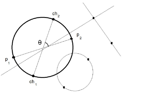
Figure 5: Proper children’s choice

Conditions $1_{\Lambda}-6_{\Lambda}$ are satisfied provided the modes in $\Lambda_{2}$ are not placed in certain points of the circle $C$. The number of these points is of order smaller than $60^{N}$. Indeed, we have to exclude:

• The points of the previous generation ($2^{N}$ points).

• The points of $\Lambda_{2}$ which have already been placed (at most $2^{N}$).

• To avoid the existence of more rectangles besides the nuclear families, we proceed as follows. We consider

  • all the already placed points,

  • all the lines perpendicular to lines containing two of these points and passing through one of them,

  • all the circles having as a diameter the segment between two of the already placed points (see Figure 5).

  Call $\mathcal{L}$ the set of these lines and $\mathcal{C}$ the set of these circles. The cardinality $|\mathcal{L}\cup\mathcal{C}|$ is at most of order $5^{N}$. Then, we have to exclude all the intersections between any object in $\mathcal{L}\cup\mathcal{C}$ with the circle $C$.

• To ensure that condition $6_{\Lambda}$ is satisfied, we consider the set $\mathcal{P}$ of the points which are the intersection between any two objects in $\mathcal{L}\cup\mathcal{C}$. It is easy to see that $|\mathcal{P}|$ is of order at most $25^{N}$. Consider the sets

  • $\mathcal{L}^{\prime}$ containing the lines which are perpendicular to a line containing a point in $\mathcal{P}$ and an already placed point of $\Lambda$, and contain one of these two points,

  • $\mathcal{C}^{\prime}$ containing the circles having as a diameter a segment whose endpoints are a point in $\mathcal{P}$ and an already placed point of $\Lambda$.

  The cardinality $|\mathcal{L}^{\prime}\cup\mathcal{C}^{\prime}|$ is at most of order $60^{N}$. Then, we have to exclude also the intersections between an element in $\mathcal{L}\cup\mathcal{C}$ and $C$.

We can place the children of the nuclear family at rational points of the circle $C$ away from the ones just mentioned. To estimate its denominator we apply our estimate on the number of the Pythagorean triples. We have that the number of $\theta$’s with slopes whose tangent is given by a rational whose numerator and denominator is bounded by $R$ lower bounded by $\sqrt{R/2}-1$. Thus, we can choose $R=60^{2N}$. Formula $\tan(\alpha+\beta)=(\tan\alpha+\tan\beta)/(1+\tan\alpha\tan\beta)$ implies that $Q_{2}\leq 2\,60^{2N}\,Q_{1}$. Thus, denominators and numerators in $\Lambda_{1}\cup\Lambda_{2}$ are upper bounded by $Q_{2}$. This grid is accurate enough to place the pairs of $\Lambda_{2}$ in the corresponding circles. Iteratively, we can place the following generations refining the grid at each step by dealing with Gaussian rationals whose (co)tangent has numerator and denominator bounded by $60^{3jN}$ at the $j$ generation. Therefore, after placing the $N$ generations and mapping the set $\Lambda$ from $\mathbb{Q}[i]$ to $\mathbb{Z}[i]$ we obtain that all the modes $n\in\Lambda$ satisfy

$$|n|\lesssim 60^{3N^{2}}.$$

This procedure can be done so that the final configuration of modes is close to the prototype embedding in [CKS⁺10] to ensure that condition (15) is satisfied. Finally, to obtain the estimate (119), it is enough to take any $B\geq 60^{4}$.

Appendix D Notations

• $\mathcal{K}$ — growth of the Sobolev norm of the solution $\|u(t)\|_{H^{s}}$ from Theorem 1;

• $s$ — index of the Sobolev space.

• $\mathcal{H}$ — the Hamiltonian of (1), defined in (9);

• $\mathcal{D}$ — quadratic part of the Hamiltonian $\mathcal{H}$ defined in (9);

• $\mathcal{G}$ — quartic part of the Hamiltonian $\mathcal{H}$ defined in (9);

• $\mathcal{M}$ — abusing notation, mass of both the solutions of the equation (1) and of the toy model (18)

• $\{a_{n}(t)\}_{n\in\mathbb{Z}^{2}}$ — Fourier coefficients of the solutions of (1) or, equivalently, solution of system $\dot{a}_{n}=2\,i\,\partial_{\overline{a_{n}}}\mathcal{H}$;

• $\Gamma$ — normal form change for the Hamiltonian (9). It is given in Theorem 2.

• $\widetilde{\mathcal{G}}$ — resonant terms of $\mathcal{G}$.

• $\mathcal{R}$ — remainder (of degree 5) of the Hamiltonian $\mathcal{H}$ after performing one step of normal form, that is remainder of the Hamiltonian $\mathcal{H}\circ\Gamma$.

• $\{\alpha_{n}(t)\}_{n\in\mathbb{Z}^{2}}$ — Solutions of the normalized Hamiltonian $\mathcal{H}\circ\Gamma$, given in Theorem 2;

• $\mathcal{A}_{0}(n)\subset(\mathbb{Z}^{2})^{3}$ — collection of the resonance convolutions defined in (11);

• $\{\beta_{n}(t)\}_{n\in\mathbb{Z}^{2}}$ — rotated fourier coefficients, $\beta_{n}=\alpha_{n}e^{-i(G+|n|^{2})t}$. They satisfy (14).

• $\mathcal{A}(n)\subset(\mathbb{Z}^{2})^{3}$ — collection of reduced resonance convolutions defined after (14);

• $N-4$ — number of energy cascades;

• $\Lambda\subset\mathbb{Z}^{2}$ essential Fourier coefficients given as a disjoint union of $N$ pairwise disjoint generations: $\Lambda=\Lambda_{1}\cup\cdots\Lambda_{N}$. See Proposition 3.1 and preceding discussion.

• $\{b_{j}(t)\}_{j=1}^{N}$ solution to the Toy Model (18);

• $h(b)$ — Hamiltonian of the Toy Model, given in (19);

• $\mathbb{T}_{j}$ — periodic orbits of the Toy Model (18)

• $\{c^{(j)}_{k}\}_{k\neq j}$ — coordinates adapted to the periodic orbit $\mathbb{T}_{j}$ after symplectic reduction, given in Section 4.1.

• $(p_{1},q_{1},p_{2},q_{2})$ — hyperbolic variables adapted to the periodic orbit $\mathbb{T}_{j}$ after diagonalization, given in Section 4.1.

• $\mathcal{Z}_{\mathrm{hyp},*},\mathcal{Z}_{\ell,*},\mathcal{Z}_{\mathrm{mix},*}$ — types of remainder terms of the original Hamiltonian $H$ after symplectic reduction and diagonalization near the periodic orbit $\mathbb{T}_{j}$. Subscript means hyperbolic, elliptic and mixed remainder respectively (see Lemma 4.1).

• $\Sigma_{j}^{\mathrm{in}}$ — transversal section to the stable manifold of $\mathbb{T}_{j}$, defined in (56)

• $\Sigma_{j}^{\mathrm{out}}$ — transversal section to the unstable manifold of $\mathbb{T}_{j}$, defined in (64)

• $\mathcal{B}^{j}$ — map from $\Sigma_{j}^{\mathrm{in}}$ to $\Sigma_{j+1}^{\mathrm{in}}$ given by the flow of the Toy Model (18) (see Section 4).

• $\mathcal{B}^{j}_{\mathrm{loc}}$ — local map from $\Sigma_{j}^{\mathrm{in}}$ to $\Sigma_{j}^{\mathrm{out}}$ given by the flow of (18), defined in (65).

• $\mathcal{B}^{j}_{\mathrm{glob}}$ — global map from $\Sigma_{j}^{\mathrm{out}}$ to $\Sigma_{j+1}^{\mathrm{in}}$ given by the flow (18), defined in (66).

• $a=\mathcal{O}(b)$ means $|b|<Ka$ for some $K$ independent of $\delta,\sigma,N,j$.

• $a=\mathcal{O}_{\sigma}(b)$ means $|b|<Ka$ for some $K$ independent of $\delta,N,j$.

• $\Psi_{\mathrm{hyp}}$ — the change of coordinates for the hyperbolic toy model (see Lemma 5.1).

• $\Psi$ — the change of coordinates for the full toy model (see Lemma 6.1).

• $R_{\mathrm{hyp},*}$, $R_{\mathrm{mix},*}$, $,\mathcal{Z}_{\ell,*}$ — collection of remainder terms for the Full Toy Model after normal form transformation $\Psi$ (see Lemma 6.1).

• $\mathcal{V}_{j}\subset\Sigma_{j}^{\mathrm{in}}$ — an open subset contained in the domain of definition of $\mathcal{B}^{j}_{\mathrm{loc}}$ so that $\mathcal{B}^{j}_{\mathrm{loc}}(\mathcal{V}_{j})\subset\mathcal{U}_{j}$.

• $\mathcal{U}_{j}\subset\Sigma_{j}^{\mathrm{out}}$ — an open subset contained in the domain of definition of $\mathcal{B}^{j}_{\mathrm{glob}}$ so that $\mathcal{B}^{j}_{\mathrm{glob}}(\mathcal{U}_{j})\subset\mathcal{V}_{j+1}$.

• $\mathcal{N}_{j}^{\pm}$ — initial conditions inside $\Sigma^{\mathrm{in}}_{j}$ whose orbits under the flow $\Phi^{t}$ have cancellation property (see Lemma 5.2)

• $\mathcal{W}_{j}$ — an auxiliary set in the $(p,q,c)$–space (see Corollary 7.2)

• $g_{\mathcal{I}_{j}}(p_{2},q_{2},\sigma,\delta)$ — the cancellation function, defined in (94) and used in the definition of $\mathcal{N}_{j}^{\pm}$.

• $T_{0}$ — time of evolution of the Toy Model in Theorem 3.

• $\gamma$ — constant which gives the relation between $\delta$ and $N$.

• $\mathbb{K}$ — constant from upper bound on time in Theorem 3.

• $\lambda$ — rescaling parameter see (21);

• $\kappa$ — constant wich gives the relation between $\lambda$ and $N$.

• $T$ — time of evolution after rescaling, see (22);

• $\{b^{\lambda}_{j}(t)\}_{j=1}^{N}$ rescaled solution to the Toy Model, given in (21);

• $\{\beta^{\lambda}_{n}(t)\}_{n\in\mathbb{Z}^{2}}$ the lift of the above solution to the Toy Model to approximate solution to (14);

References

- [Bam97] D. Bambusi. Long time stability of some small amplitude solutions in nonlinear Schrödinger equations. Comm. Math. Phys., 189(1):205–226, 1997.
- [Bam99] D. Bambusi. Nekhoroshev theorem for small amplitude solutions in nonlinear Schrödinger equations. Math. Z., 230(2):345–387, 1999.
- [Bam03] D. Bambusi. Birkhoff normal form for some nonlinear PDEs. Comm. Math. Phys., 234(2):253–285, 2003.
- [BB11] M. Berti and L. Biasco. Branching of Cantor manifolds of elliptic tori and applications to PDEs. Comm. Math. Phys., 305(3):741–796, 2011.
- [Ber07] M. Berti. Nonlinear oscillations of Hamiltonian PDEs. Progress in Nonlinear Differential Equations and their Applications, 74. Birkhäuser Boston Inc., Boston, MA, 2007.
- [BG06] D. Bambusi and B. Grébert. Birkhoff normal form for partial differential equations with tame modulus. Duke Math. J., 135(3):507–567, 2006.
- [BK92] I. U. Bronsteĭn and A. Ya. Kopanskiĭ. Finitely smooth normal forms of vector fields in the vicinity of a rest point [ MR1167014 (93j:58120)]. In Global analysis—studies and applications, V, volume 1520 of Lecture Notes in Math., pages 157–172. Springer, Berlin, 1992.
- [BK94] I. U. Bronstein and A. Ya. Kopanskiĭ. Smooth invariant manifolds and normal forms, volume 7 of World Scientific Series on Nonlinear Science. Series A: Monographs and Treatises. World Scientific Publishing Co. Inc., River Edge, NJ, 1994.
- [Bou93] J. Bourgain. Fourier transform restriction phenomena for certain lattice subsets and application to nonlinear evolution equations. i. schrödinger equations. Geom. Funct. Anal., 3(2):107–156, 1993.
- [Bou96] J. Bourgain. On the growth in time of higher Sobolev norms of smooth solutions of Hamiltonian PDE. Internat. Math. Res. Notices, 6:277–304, 1996.
- [Bou98] J. Bourgain. Quasi-periodic solutions of Hamiltonian perturbations of 2D linear Schrödinger equations. Ann. of Math. (2), 148(2):363–439, 1998.
- [Bou00a] J. Bourgain. On diffusion in high-dimensional Hamiltonian systems and PDE. J. Anal. Math., 80:1–35, 2000.
- [Bou00b] J. Bourgain. Problems in Hamiltonian PDE’s. Geom. Funct. Anal., Special Volume, Part I:32–56, 2000. GAFA 2000 (Tel Aviv, 1999).
- [Bou04] J. Bourgain. Remarks on stability and diffusion in high-dimensional Hamiltonian systems and partial differential equations. Ergodic Theory Dynam. Systems, 24(5):1331–1357, 2004.
- [CDKS01] J. E. Colliander, J.-M. Delort, C. E. Kenig, and G. Staffilani. Bilinear estimates and applications to 2D NLS. Trans. Amer. Math. Soc., 353(8):3307–3325 (electronic), 2001.
- [CE10] R. Carles and Faou E. Energy cascade for nls on . page 15 pp. Arxiv: 1010.5173v1, 2010.
- [CKO12] J. Colliander, S. Kwon, and T. Oh. A remark on normal forms and the upside-down I-method for periodic NLS: growth of higher Sobolev norms. Preprint available at http://arxiv.org/abs/1010.2501, 2012.
- [CKS+10] J. Colliander, M. Keel, G. Staffilani, H. Takaoka, and T. Tao. Transfer of energy to high frequencies in the cubic defocusing nonlinear Schrödinger equation. Invent. Math., 181(1):39–113, 2010.
- [CW93] W. Craig and C.E. Wayne. Newton’s method and periodic solutions of nonlinear wave equations. Comm. Pure Appl. Math., 46(11):1409–1498, 1993.
- [CW10] F. Catoire and W.-M. Wang. Bounds on Sobolev norms for the defocusing nonlinear Schrödinger equation on general flat tori. Commun. Pure Appl. Anal., 9(2):483–491, 2010.
- [EK10] L. H. Eliasson and S. B. Kuksin. KAM for the nonlinear Schrödinger equation. Ann. of Math. (2), 172(1):371–435, 2010.
- [Fen77] N. Fenichel. Asymptotic stability with rate conditions. II. Indiana Univ. Math. J., 26(1):81–93, 1977.
- [Fen74] N. Fenichel. Asymptotic stability with rate conditions. Indiana Univ. Math. J., 23:1109–1137, 1973/74.
- [GG10] P. Gérard and S. Grellier. The cubic Szegő equation. Ann. Sci. Éc. Norm. Supér. (4), 43(5):761–810, 2010.
- [GIP09] B. Grébert, R. Imekraz, and E. Paturel. Normal forms for semilinear quantum harmonic oscillators. Comm. Math. Phys., 291(3):763–798, 2009.
- [GKP12] B. Grébert, T. Kappeler, and J. Pöschel. Normal form theory for the NLS equation. Preprint available at http://arxiv.org/abs/0907.39381, 2012.
- [Han11] Z. Hani. Global and dynamical aspects of nonlinear schrödinger equations on compact manifolds. Ph. D. thesis UCLA, 2011.
- [HPS77] M.W. Hirsch, C.C. Pugh, and M. Shub. Invariant manifolds, volume 583 of Lecture Notes in Math. Springer-Verlag, Berlin, 1977.
- [KLS11] V. Kaloshin, M. Levi, and M. Saprykina. Arnold diffusion in a pendulum lattice. In preprint, page 22pp. 2011.
- [KP96] S. Kuksin and J. Pöschel. Invariant Cantor manifolds of quasi-periodic oscillations for a nonlinear Schrödinger equation. Ann. of Math. (2), 143(1):149–179, 1996.
- [KP03] T. Kappeler and J. Pöschel. KdV & KAM. Springer-Verlag, Berlin, 2003.
- [Kuk93] S.B. Kuksin. Nearly integrable infinite-dimensional Hamiltonian systems, volume 1556 of Lecture Notes in Mathematics. Springer-Verlag, Berlin, 1993.
- [Kuk95] S. B. Kuksin. On squeezing and flow of energy for nonlinear wave equations. Geom. Funct. Anal., 5(4):668–701, 1995.
- [Kuk96] S. Kuksin. Growth and oscillations of solutions of nonlinear Schrödinger equation. Comm. Math. Phys., 178(2):265–280, 1996.
- [Kuk97a] S. B. Kuksin. On turbulence in nonlinear Schrödinger equations. Geom. Funct. Anal., 7(4):783–822, 1997.
- [Kuk97b] S. B. Kuksin. Oscillations in space-periodic nonlinear Schrödinger equations. Geom. Funct. Anal., 7(2):338–363, 1997.
- [Kuk99] S. B. Kuksin. Spectral properties of solutions for nonlinear PDEs in the turbulent regime. Geom. Funct. Anal., 9(1):141–184, 1999.
- [Poc11] O. Pocovnicu. Explicit formula for the solution of the Szegö equation on the real line and applications. Discrete Contin. Dyn. Syst., 31(3):607–649, 2011.
- [Poc12] O. Pocovnicu. First and second order approximations for a nonlinear wave equation. Preprint available at http://arxiv.org/abs/1111.6060, 2012.
- [PP12] C. Procesi and M. Procesi. Normal Form for the Schrödinger equation with analytic non–linearities. Preprint available at http://arxiv.org/abs/1012.0446, 2012.
- [Rab78] P. H. Rabinowitz. Free vibrations for a semilinear wave equation. Comm. Pure Appl. Math., 31(1):31–68, 1978.
- [Šil67] L. P. Šil′nikov. On a problem of Poincaré-Birkhoff. Mat. Sb. (N.S.), 74 (116):378–397, 1967.
- [Soh10a] V. Sohinger. Bounds on the growth of high Sobolev norms of solutions to 2D Hartree Equations. Preprint available at http://arxiv.org/abs/1003.5709, 2010.
- [Soh10b] V. Sohinger. Bounds on the growth of high Sobolev norms of solutions to Nonlinear Schrodinger Equations on . Preprint available at http://arxiv.org/abs/1003.5707, 2010.
- [Soh11] V. Sohinger. Bounds on the growth of high Sobolev norms of solutions to nonlinear Schrödinger equations on . Differential Integral Equations, 24(7-8):653–718, 2011.
- [Sta97a] G. Staffilani. On the growth of high sobolev norms of solutions for kdv and schrödinger equations. Duke Math Journal, 86(1):109–42, 1997.
- [Sta97b] G. Staffilani. Quadratic forms for a -D semilinear Schrödinger equation. Duke Math. J., 86(1):79–107, 1997.
- [Way90] C.E. Wayne. Periodic and quasi-periodic solutions of nonlinear wave equations via kam theory. Comm. Math. Phys., 127(3):479–528, 1990.
- [Zho08] S. Zhong. The growth in time of higher Sobolev norms of solutions to Schrödinger equations on compact Riemannian manifolds. J. Differential Equations, 245(2):359–376, 2008.
- [ZS71] V. E. Zakharov and A. B. Shabat. Exact theory of two-dimensional self-focusing and one-dimensional self-modulation of waves in nonlinear media. Ž. Èksper. Teoret. Fiz., 61(1):118–134, 1971.