Fermions and Kaluza–Klein vacuum decay:
a toy model

Abstract

We address the question of whether or not fermions with twisted periodicity condition suppress the semiclassical decay of $M^{4}\times S^{1}$ Kaluza–Klein vacuum. We consider a toy (1+1)-dimensional model with twisted fermions in cigar-shaped Euclidean background geometry and calculate the fermion determinant. We find that contrary to expectations, the determinant is finite. We consider this as an indication that twisted fermions do not stabilize the Kaluza–Klein vacuum.

Keywords: Kaluza-Klein theory, semiclassical vacuum decay, twisted fermions, 2-dimensional model.

1 Introduction

It is known that $M^{4}\times S^{1}$ Kaluza–Klein vacuum is unstable [1]. The vacuum decay proceeds through the Euclidean bounce, whose metric is

$$ds^{2}=\frac{d\xi^{2}}{1-\frac{R^{2}}{\xi^{2}}}+\xi^{2}d\Omega^{2}+R^{2}\left(1-\frac{R^{2}}{\xi^{2}}\right)d\theta^{2}\;,$$ (1)

where $R<\xi<\infty$, $0\leq\theta<2\pi$ and $d\Omega^{2}$ is the metric of unit 3-sphere. At large $\xi$, the geometry of this solution is $R^{4}\times S^{1}$, whereas as $\xi\rightarrow R$, the geometry approaches $R^{2}\times S^{3}$. The latter property is seen by performing the change of variables $\xi=R+\frac{r^{2}}{2R}$, which gives near $r=0$

$$ds^{2}=dr^{2}+r^{2}d\theta^{2}+R^{2}d\Omega^{2}\;.$$ (2)

Upon continuation to the space-time of Minkowskian signature, the bounce (1) describes the decay of $M^{4}\times S^{1}$ into nothing [1]. The decay of the Kaluza–Klein vacuum and similar processes are of interest from several viewpoints, and various versions of this phenomenon have been extensively discussed in literature [3, 4, 5, 6, 7, 8, 9, 10, 12, 11, 13, 14, 15].

It has been argued in Ref.[1] that $M^{4}\times S^{1}$ Kaluza–Klein vacuum is stabilized in a theory containing fermions with twisted periodicity condition in the compact coordinate,

$$\psi(\theta)=e^{-2i\pi q}\psi(\theta+2\pi)\;.$$ (3)

The argument is that in the background of the bounce (1), this condition makes perfect sense away from $\xi=R$, but for generic $q$ it appears singular at $\xi=R$. The way to see the effect of fermions on the Kaluza–Klein vacuum decay would be to calculate the ratio of fermion determinants in the background (1) and in the background of the original Kaluza–Klein metric, both with periodicity condition (3):

$$\Lambda(q)\equiv\frac{\det\mathcal{D}^{bounce}_{q}}{\det\mathcal{D}^{vacuum}_{q}}\;,$$ (4)

where $\mathcal{D}$ is the Dirac operator and index $q$ refers to the condition (3). If this ratio vanishes, the vacuum is stabilized indeed.

In this paper we consider a toy model for this situation. Namely, instead of studying the five-dimensional theory with the metric (1), we discuss two-dimensional theory with the metric describing a sigar-shaped space:

$$ds^{2}=\frac{d\xi^{2}}{1-\frac{R^{2}}{\xi^{2}}}+R^{2}\left(1-\frac{R^{2}}{\xi^{2}}\right)d\theta^{2}$$ (5)

In other words, we disregard the $S^{3}$ part of the geometry. Likewise, instead of the five-dimensional Kaluza–Klein vacuum we consider $(1+1)$-dimensional theory with the spatial dimension compactified to a circle, whose Euclidean counterpart is described by the metric

$$ds^{2}_{vac}=d\xi^{2}+R^{2}d\theta^{2}\;.$$ (6)

The metrics (5) and (6) coincide as $\xi\rightarrow\infty$, but the geometry (5) has a smooth end at $\xi=R$, just like in the case of the five-dimensional bounce. We impose the periodicity condition (3) on the two-dimensional fermions, which again makes sense away from $\xi=0$ but appears singular at $\xi=R$. Thus, we argue that our toy model captures the main features of the five-dimensional Kaluza–Klein theory, which are relevant for the vacuum decay. Our purpose is to calculate the ratio (4) in this toy model. In our calculations we consider the interval

$$R<\xi<T\;,$$ (7)

where $T$ is sent to infinity in the very end of the calculation. We do this for the determinants in the backgrounds of both “bounce” metric (5) and “vacuum” one (6). The choice of one and the same IR cutoff $T$ in these two cases mimics the five-dimensional situation, where $\xi$ is unambiguously defined as the radius of the 3-sphere both for the bounce solution and Kaluza–Klein metric.

To simplify things further, we consider massless fermions. The motivation is that a pathology, if any, in the fermion behavior in the background metric (5) would emerge from a small vicinity of the point $\xi=R$, while the short-distance properties of fermions should not be sensitive to their mass. The advantage is that we can utilize conformal invariance of massless two-dimensional fermions (modulo conformal anomaly, which is local, and therefore independent of $q$). Indeed, our metric (5), as any other $2D$ metric, is conformally flat,

$$ds^{2}=\Phi^{2}(r)[dr^{2}+r^{2}d\theta^{2}]\;,$$ (8)

where

$$r=2\;\sqrt{\frac{\xi-R}{\xi+R}}\;e^{\frac{\xi-R}{R}}\;,$$ (9)

$$\Phi=R\frac{\xi+R}{2\xi}\;e^{-\frac{\xi-R}{R}}\;.$$ (10)

Thus, instead of calculating the fermionic determinant in the background metric (5) we are going to perform the calculation on a plane, still with the periodicity condition (3).

It is worth noting that the calculation of $\det\mathcal{D}^{bounce}_{q}$ is equivalent to the calculation of the determinant for conventional (periodic) massless fermions of charge $(-q)$ in the background of an instanton in the two-dimensional Abelian Higgs model, in the limit of vanishing instanton size. If there is no interaction of fermions with the scalar field, then the fermionic part of the Lagrangian in the latter model has the form

$$\mathcal{L}_{\psi}=i\bar{\psi}\gamma^{\mu}(\partial_{\mu}-iqeA_{\mu})\psi\;,$$ (11)

while in the limit of vanishing instanton size, the field of the instanton — Abrikosov–Nielsen–Olesen vortex [16, 17] — has the Aharonov–Bohm form, $A_{\mu}=e^{-1}\partial_{\mu}\theta$. The field $\psi$ obeys the periodicity condition $\psi(\theta+2\pi)=\psi(\theta)$, so the change of variables $\psi\to e^{iq\theta}\psi$ reduces the problem to the calculation of the fermion determinant on $R^{2}$ without the gauge field background, but with the twisted condition (3).

Determinants in the instanton background are well studied in $(1+1)$ dimensional models. For scalar and vector fields the calculation was performed, for example, in Ref.[18], and for fermions in Refs.[19, 20]. In Refs.[21, 22], the calculations were performed for chiral fermions of half-integer charge, coupled to the scalar field. Interestingly, the determinants of fermions with half-integer charge do not show any pathology [21, 22].

Somewhat surprisingly, in this paper we show that similar result holds in our problem: the fermion determinant in the background of our toy “bounce” is finite for arbitrary $q\neq\pm 1/2$. We consider this as an indication that twisted fermions do not, in fact, stabilize the $M^{4}\times S^{1}$ Kaluza–Klein vacuum.

2 Fermion determinants

It is convenient to split the quantity of interest, the logarithm of the ratio (4), as follows:

$$\ln\Lambda(q)=\ln\left[\frac{\det\mathcal{D}^{bounce}_{q}}{\det\mathcal{D}^{bounce}_{q=0}}\right]-\ln\left[\frac{\det\mathcal{D}^{vacuum}_{q}}{\det\mathcal{D}^{vacuum}_{q=0}}\right]+\ln\left[\frac{\det\mathcal{D}^{bounce}_{q=0}}{\det\mathcal{D}^{vacuum}_{q=0}}\right]\;.$$ (12)

According to the above discussion, we are going to calculate $\det\mathcal{D}^{bounce}$ on a plane, and $\det\mathcal{D}^{vacuum}$ on a cylinder (6). For $q=0$, the fermion behavior in the background metric (5) is manifestly healthy, so the last term must be finite. The explicit demonstration of the latter fact is somewhat subtle; we give the corresponding analysis in Appendix.

Let us concentrate on the first two terms in the right hand side of eq. (12). Let us note that $\Lambda(q)$ is periodic in $q$ with period 1, so we can consider, without loss of generality, the range $-1/2<q\leq 1/2$. Furthermore, due to $C$-invariance, $\Lambda(q)$ is symmetric under $q\to-q$. Therefore, it is sufficient to study the theory with $0\leq q\leq 1/2$. We are going to perform our calculation for

$$0\leq q<\frac{1}{2}\;.$$ (13)

The case $q=1/2$ is subtle for reasons that will become clear later, and we leave it for the future.

2.1 Vacuum background

We begin with the vacuum-vacuum term. We recall that

$$\ln\left[\det\mathcal{D}^{vacuum}_{q}\right]=-E_{q}T\;,$$ (14)

where $T$ is the normalization time and $E_{q}$ is the Casimir energy of fermions with twisted periodicity condition in the $R^{1}\times S^{1}$ theory. This Casimir energy was calculated in Ref. [2], but the resulting expression there is somewhat implicit. So, we redo the calculation here. We write the Casimir energy as a sum over energies of the Dirac sea levels,

$$E_{q}=-\sum_{n=-\infty}^{\infty}\omega_{n}(q)\;,$$ (15)

where $n$ is the angular spectral number and $\omega_{n}=|n+q|/R$. We regularize this sum by multiplying each term by a factor $\exp(-\varepsilon|\omega_{n}(q)|)$, where $\varepsilon$ is a small parameter sent to zero in the end of the calculation, and obtain

$$E_{q}-E_{0}=-\frac{1}{R}\left[\sum_{n=-\infty}^{\infty}|n+q|e^{-\varepsilon|n+q|}-\sum_{n=-\infty}^{\infty}|n|e^{-\varepsilon|n|}\right]\;.$$ (16)

With our convention (13), this sum is straightforwardly evaluated, and in the limit $\varepsilon\rightarrow 0$ we obtain

$$\ln\left[\frac{\det\mathcal{D}^{vacuum}_{q}}{\det\mathcal{D}^{vacuum}_{0}}\right]=-(E_{q}-E_{0})T=-\frac{T}{R}(q^{2}-q)$$ (17)

We have compared numerically this simple result with that of Ref. [2] and found excellent agreement.

2.2 Bounce background

Let us now turn to the bounce-bounce term in Eq. (12), which involves the ratio of determinants on a disc $r\leq a$, where $a$ is the IR cutoff in terms of the coordinate $r$, cf. Eq. (7). As the operator $\mathcal{D}^{bounce}$ is anti-Hermitean, its eigenvalues are purely imaginary:

$$\ln\det\mathcal{D}^{bounce}=\sum\limits_{l,m}\ln(i\lambda_{l,m})\;,$$ (18)

where $l$ and $m$ are the radial and angular spectral numbers, respectively, and $\lambda_{l,m}$ are the eigenvalues of the operator $\mathcal{D}^{bounce}$,

$$\mathcal{D}^{bounce}\psi_{l,m}=\gamma^{\mu}\partial_{\mu}\psi_{l,m}=i\lambda_{l,m}\psi_{l,m}\;.$$ (19)

We take Euclidean $\gamma$-matrices and spinors in the following form:

$$\gamma^{0}=\begin{pmatrix}0&1\\ 1&0\end{pmatrix},\qquad\gamma^{1}=\begin{pmatrix}0&-i\\ i&0\end{pmatrix},\qquad\psi=\begin{pmatrix}\phi\\ \chi\end{pmatrix}$$

and impose the Dirichlet boundary conditions in the radial coordinate,

$$\phi(a,\theta)=0\;.$$ (20)

We require that the eigenfunctions $\psi_{l,m}$ be square-integrable.

The component $\chi$ is related to $\phi$ as follows,

$$\chi=\frac{1}{i\lambda}(\partial_{0}\phi+i\partial_{1}\phi)\;,$$ (21)

while $\phi$ obeys

$$\Delta\phi=-\lambda^{2}\phi$$ (22)

The eigenfunctions are

$$\phi_{l,m}(r,\theta)=\mbox{e}^{im\theta}\phi_{l,m}(r)\;,$$ (23)

where

$$m=n+q$$ (24)

and $n$ is integer. $\phi_{l,m}(r)$ obeys the Bessel equation

$$r^{2}\phi_{l,m}^{\prime\prime}+r\phi_{l,m}^{\prime}+[\lambda_{l,m}^{2}r^{2}-m^{2}]\phi_{l,m}=0\;.$$ (25)

Obviously, the eigenvalues come in pairs, $\pm\lambda_{l,m}$, where $\lambda_{l,m}>0$. Note, that $\mathcal{D}^{bounce}$ has no zero mode: even though for $\lambda=0$ both $\phi$ and $\chi$ can be square-integrable, it is impossible to satisfy the boundary condition (20). So, we have

$$\ln[\det\mathcal{D}^{bounce}]=\sum_{\lambda_{l,m}>0}\ln\lambda_{l,m}^{2}\;.$$

The square-integrable solutions are $\phi_{l,m}=\operatorname{J}_{m}(r\lambda_{m})=\operatorname{J}_{n+q}(r\lambda_{n+q})$ for $n\geq 0$ and $\phi_{l,m}=\operatorname{J}_{-m}(r\lambda_{-m})=\operatorname{J}_{-n-q}(r\lambda_{-n-q})$ for $n\leq-1$. It is convenient to rewrite the latter function as $\operatorname{J}_{n^{\prime}-q}(r\lambda_{n^{\prime}-q})$, where $n^{\prime}\geq 1$; in what follows $m_{q}$ denotes either $n+q$ or $n^{\prime}-q$. It is straightforward to see that for these solutions, the components $\chi$ given by Eq. (21) are square integrable as well.

Let us point out a subtlety of the antiperiodic fermions, $q=1/2$. In that case the solutions to Eq. (19) with $n=-1$ are not square integrable: either $\phi$ or $\chi$ behaves as $r^{-1/2}$ near the origin. We leave the analysis of this case for the future, and proceed with the model with $0\leq q<1/2$.

2.2.1 Sum over radial spectral numbers

The radial spectrum of eigenvalues is determined by the following equations:

$$\operatorname{J}_{n+q}(a\lambda_{l,n+q})=0\;;\quad n\geq 0$$ (26)

$$\operatorname{J}_{n^{\prime}-q}(a\lambda_{l,n^{\prime}-q})=0\;;\quad n^{\prime}\geq 1$$ (27)

Let us evaluate the sum over radial spectral numbers $l$ for a given $n$ using $\zeta$-function method,

$$\sum_{l}\left(\ln\lambda^{2}_{l,m_{q}}-\ln\lambda^{2}_{l,m_{0}}\right)=-\frac{d}{ds}Z_{m}(s)\bigg{|}_{s=0}\;,$$

where

$$Z_{m}(s)\equiv\zeta_{m_{q}}(s)-\zeta_{m_{0}}(s)=\sum_{l=1}^{\infty}\left(\lambda_{l,m_{q}}^{-2s}-\lambda_{l,m_{0}}^{-2s}\right)$$ (28)

The direct calculation of this sum is complicated by the fact that the eigenvalues are not known analytically. To this end, a convenient tool is the Gelfand–Yaglom formalism [23, 24, 26, 25], which was successfully applied for calculations of other functional determinants.

Let us briefly describe the method. If we know a function $F(z)$ which has zeros at desired eigenvalues, which are assumed to be positive, then its logarithmic derivative has simple poles with residues equal to 1 at those eigenvaluse, and we can write $\zeta$-function as follows:

$$\zeta(s)=\sum_{l}\operatorname*{Res}\left[z^{-s}\frac{d}{dz}\ln F(z)\right]$$ (29)

Assuming that $F(z)$ is non-singular anywhere except possibly for real negative semi-axis and $z=\infty$, this can be transformed into a contour integral, see Fig. 1,

$$\zeta(s)=\zeta_{\gamma}(s)+\zeta_{\Omega}(s)\;,$$ (30)

where

$$\zeta_{\gamma}(s)=\frac{1}{2\pi i}\int\limits_{\gamma}dz\;z^{-s}\frac{d}{dz}\ln F(z)\;,$$ (31)

$$\zeta_{\Omega}(s)=\frac{1}{2\pi i}\int\limits_{\Omega}dz\;z^{-s}\frac{d}{dz}\ln F(z)\;.$$ (32)

The contour $\gamma$ surrounds the negative real semi-axis, and $\Omega$ is a large circle. The integration runs clockwise in (31) and counter-clockwise in (32).

Figure 1: The integration contour in the $z$-plane. The sum over residues (integral over small circles) equals the contour integral (30).

The first trial in our case would be $F(z)=\operatorname{J}_{m}(az)$, which has zeros at $z=\lambda_{l,m}$. However, we actually need zeros at $z=\lambda_{l,m}^{2}$. Also, we have to avoid a zero at $z=0$. The function that satisfies these requirements is

$$F(z)=\frac{\operatorname{J}_{m_{q}}(a\sqrt{z})}{(a\sqrt{z})^{m_{q}}}\;.$$ (33)

Let us first calculate the integral over the large circle,

$$Z_{m,\Omega}(s)=\frac{1}{2\pi i}\int\limits_{\Omega}dz\;z^{-s}\left(\frac{d}{dz}\ln\left[\frac{\operatorname{J}_{m_{q}}(a\sqrt{z})}{\operatorname{J}_{m_{0}}(a\sqrt{z})}\right]+\frac{d}{dz}\ln\left[a^{m_{0}-m_{q}}z^{(m_{0}-m_{q})/2}\right]\right)\;.$$ (34)

To estimate the behavior of the term containing Bessel functions, we make use of the “approximation by tangents” [27] at large $|z|$ and possibly large index $m$,

$$\operatorname{J}_{m}(z)\simeq\sqrt{\frac{2}{\pi\sqrt{z^{2}-m^{2}}}}\;\Bigg{[}\left(1-\frac{9}{128(z^{2}-m^{2})}\right)\cos\left(\sqrt{z^{2}-m^{2}}-m\arccos\frac{m}{z}-\frac{\pi}{4}\right)+\\ \left(\frac{1}{8\sqrt{z^{2}-m^{2}}}+\frac{5m^{2}}{24(z^{2}-m^{2})^{3/2}}\right)\sin\left(\sqrt{z^{2}-m^{2}}-m\arccos\frac{m}{z}-\frac{\pi}{4}\right)\Bigg{]},$$ (35)

and find that the first term in the integrand in (34) behaves as $|z|^{-3/2}$ at complex infinity. Therefore, its contribution to the integral (34) vanishes as $s\rightarrow 0$. The contribution of the second term is straightforwardly evaluated and gives

$$Z^{\prime}_{m,\Omega}(0)=\frac{m_{q}-m_{0}}{2}\ln L\;,$$ (36)

where $L$ is the radius of the large circle.

Let us turn to the remaining part, $Z_{m,\gamma}(s)$. We recall that

$$\operatorname{J}_{m}(e^{\pm i\frac{\pi}{2}}x)=e^{\pm i\frac{\pi m}{2}}\operatorname{I}_{m}(x);\quad\arg x=0\;,$$ (37)

and get

$$Z_{m,\gamma}(s)=\frac{\sin\pi s}{\pi}\int\limits_{0}^{L}dx\;x^{-s}\left(\frac{d}{dx}\ln\left[\frac{\operatorname{I}_{m_{q}}(a\sqrt{x})}{\operatorname{I}_{m_{0}}(a\sqrt{x})}\right]+\frac{d}{dx}\ln\left[a^{m_{0}-m_{q}}x^{(m_{0}-m_{q})/2}\right]\right)$$ (38)

We see that $Z^{\prime}_{m,\gamma}(0)$ is an integral of total derivative. The contribution due to the upper limit $x=L$ is proportional to $\ln L$ and exactly cancels out the contribution (36). Taking into account that $\ln\left[\operatorname{I}_{m_{q}}(a\sqrt{x})/\operatorname{I}_{m_{0}}(a\sqrt{x})\right]$ vanishes as $x\rightarrow\infty$, we finally get

$$Z^{\prime}_{m}(0)=-\lim_{x\rightarrow 0}\ln\left[\frac{\operatorname{I}_{m_{q}}(a\sqrt{x})}{\operatorname{I}_{m_{0}}(a\sqrt{x})}x^{(m_{0}-m_{q})/2}\right]=-\ln\left[\left(\frac{a}{2}\right)^{m_{q}-m_{0}}\frac{\Gamma(m_{0}+1)}{\Gamma(m_{q}+1)}\right]\;.$$ (39)

2.2.2 Sum over angular spectral numbers

We are now in a position to calculate the ratio of determinants. We regularize the sum over angular spectral numbers by multiplying the determinants by $\exp(i\varepsilon|\partial_{\theta}|)$, cf. Eq. (16), and write explicitly

$$\ln[\det\mathcal{D}^{bounce}_{q}]\exp(i\varepsilon|\partial_{\theta}|)-\ln[\det\mathcal{D}^{bounce}_{0}]\exp(i\varepsilon|\partial_{\theta}|)\\ =\sum_{n=1}^{\infty}\bigg{\{}\ln\left[\left(\frac{a}{2}\right)^{n+q-1}\Gamma^{-1}(n+q)\right]e^{-\varepsilon(n+q-1)}+\ln\left[\left(\frac{a}{2}\right)^{-(n-1)}\Gamma(n)\right]e^{-\varepsilon(n-1)}\bigg{\}}+\\ \sum_{n^{\prime}=1}^{\infty}\bigg{\{}\ln\left[\left(\frac{a}{2}\right)^{n^{\prime}-q}\Gamma^{-1}(n^{\prime}-q+1)\right]e^{-\varepsilon(n^{\prime}-q)}+\ln\left[\left(\frac{a}{2}\right)^{-n^{\prime}}\Gamma(n^{\prime}+1)\right]e^{-\varepsilon n^{\prime}}\bigg{\}}$$ (40)

where we have shifted the argument in the first sum, $n\rightarrow(n-1)$. The right hand side of Eq. (40) contains $a$-dependent and $a$-independent parts,

$$\ln[\det\mathcal{D}^{bounce}_{q}]\exp(i\varepsilon|\partial_{\theta}|)-\ln[\det\mathcal{D}^{bounce}_{0}]\exp(i\varepsilon|\partial_{\theta}|)=\sum_{n=1}^{\infty}\Delta(n,q)+\sum_{n=1}^{\infty}\tilde{\Delta}(n,q,a)\;,$$ (41)

where

$$\sum_{n=1}^{\infty}\Delta(n,q)=\sum_{n=1}^{\infty}\bigg{[}\ln\Gamma(n)e^{-\varepsilon n}+\ln\Gamma(n+1)e^{-\varepsilon(n+1)}\\ -\ln\Gamma(n+q)e^{\varepsilon(n+q)}-\ln\Gamma(n+1-q)e^{\varepsilon(n+1-q)}\bigg{]}$$ (42)

and

$$\sum_{n=1}^{\infty}\tilde{\Delta}(n,q,a)=\ln\frac{a}{2}\cdot\sum_{n=1}^{\infty}\Big{[}(n+q-1)e^{-\varepsilon(n+q-1)}-(n-1)e^{-\varepsilon(n-1)}\\ +(n-q)e^{-\varepsilon(n-q)}-ne^{-\varepsilon n}\Big{]}$$ (43)

The $a$-dependent sum, Eq. (43), coincides with that of Section 2.1, and we immediately obtain that in the limit $\varepsilon\to 0$ this term is

$$\sum_{n=1}^{\infty}\tilde{\Delta}(n,q,a)=(q-q^{2})\ln\frac{a}{2}$$ (44)

We now recall that $r=a$ is the cutoff radius on a plane, which is related to the cutoff $\xi=T$ by Eq. (9), i.e., $\ln(a/2)=T/R$. Thus, the contribution (44) cancels out the second term in Eq. (12), which is given by Eq. (17). As could have been anticipated, the result for $\ln\Lambda(q)$ is infrared finite.

The quantity of interest, $\ln\Lambda(q)$, is thus given entirely by the $a$-independent sum (42) (modulo the last, $q$-independent term in Eq. (12)). To extract its part which is potentially divergent in the limit $\varepsilon\to 0$, we make use of the Stirling approximation,

$$\ln\Gamma(n)=\left[\ln\Gamma(n)\right]_{St}+O(n^{-3})\;,$$

where

$$\left[\ln\Gamma(n)\right]_{St}=n\ln n-n-\frac{1}{2}\ln n+\frac{1}{2}\ln 2\pi+\frac{1}{12n}\;.$$ (45)

Hereafter the subscript $St$ denotes the quantities calculated within the Stirling approximation. Since $\Delta(n)-\Delta_{St}(n)$ decreases as $n^{-3}$ at large $n$, potentially dangerous are the sums involving the Stirling approximation of $\ln\Gamma(n)$. These boil down to

$$\sum_{n=1}^{\infty}e^{-\varepsilon n}n\ln n=-\frac{d}{ds}\operatorname{Li}_{s}(e^{-\varepsilon})\bigg{|}_{s=-1}\;,$$ (46)

$$\sum_{n=1}^{\infty}e^{-\varepsilon n}\ln n=-\frac{d}{ds}\operatorname{Li}_{s}(e^{-\varepsilon})\bigg{|}_{s=0}\;,$$ (47)

$$\sum_{n=1}^{\infty}\frac{e^{-\varepsilon n}}{n}=-\ln(1-e^{-\varepsilon})\;,$$ (48)

where $\operatorname{Li}_{s}(z)$ is polylogarithm. We find that the terms that diverge as $\varepsilon\to 0$ actually cancel out due to the identity

$$\lim_{\varepsilon\rightarrow 0}\left(\varepsilon^{2}\frac{d}{ds}\operatorname{Li}_{s}(e^{-\varepsilon})\bigg{|}_{s=-1}-2\varepsilon\frac{d}{ds}\operatorname{Li}_{s}(e^{-\varepsilon})\bigg{|}_{s=0}+\ln(1-e^{-\varepsilon})\right)=-1-\gamma\;,$$ (49)

where $\gamma$ is the Euler–Mascheroni constant. Thus, the ratio of fermion determinants, $\Lambda(q)$ is finite, which is our main result. The explicit expression is

$$\ln\left[\frac{\det\mathcal{D}^{bounce}_{q}}{\det\mathcal{D}^{bounce}_{0}}\right]-\ln\left[\frac{\det\mathcal{D}^{vacuum}_{q}}{\det\mathcal{D}^{vacuum}_{0}}\right]\\ =\gamma(q-q^{2})+\frac{1}{12}\left(2\gamma-1+\psi(1+q)+\psi(2-q)\right)+\sum_{n=1}^{\infty}(\Delta(n,q)-\Delta_{St}(n,q))\;,$$ (50)

modulo finite and $q$-independent constant. The leading contribution here comes from the analytical part. This function is shown in Fig. 2.

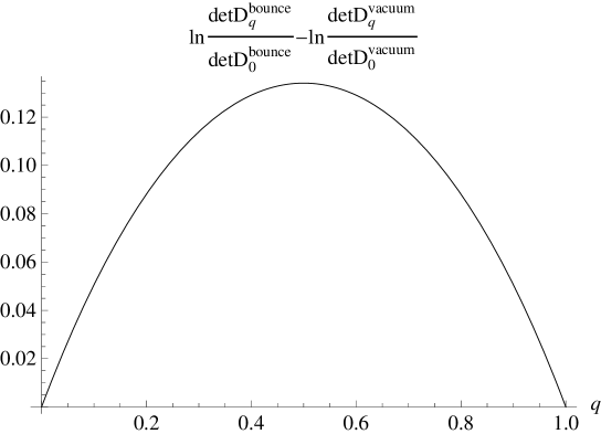
Figure 2: Logarithm of the fermion determinant as function of the twist $q$.

To summarize, we have found that all would-be divergences cancel out, and the determinant of twisted fermions is finite in the background of our “bounce”. Were similar situation inherent in the five-dimensional theory, the Kaluza–Klein vacuum would be unstable even in the presence of twisted fermions.

Appendix

Let us show that the last term in Eq. (12), corresponding to periodic fermions, is finite. We begin with the vacuum term and again use Eq. (14), now with $q=0$. We write

$$E=-\frac{2}{R}\sum_{n=1}^{\infty}n\mbox{e}^{-\varepsilon n}\;,$$

where $\varepsilon$ is the regularization parameter. It is straightforward to obtain

$$E=-\frac{2}{R\varepsilon^{2}}+\frac{1}{6R}\;.$$

The interpretation of the first, divergent term is that it corresponds to the vacuum energy density on infinite line, which should be renormalized away. Indeed, physically meaningful is the cutoff in energy, $\mbox{exp}(-\omega_{n}/\Lambda)$. Since $\omega_{n}=|n|/R$, we identify $\varepsilon=(\Lambda R)^{-1}$, and the first term becomes $E=-2\Lambda^{2}R$. The corresponding energy density $E/R$ is independent of $R$, so it is indeed the energy density on a line. So, the Casimir energy of periodic massless fermions equals

$$E=\frac{1}{6R}\;.$$

Let us consider now the bounce term. We introduce the notation $\omega(r;R)=\ln\Phi(r;R)$, and consider the variation of the determinant under the change of the value of $R$. The conformal anomaly gives [28, 29]

$$\delta_{R}\ln\det\mathcal{D}_{0}^{bounce}=-\frac{1}{6\pi}\int\leavevmode\nobreak\ d^{2}x\leavevmode\nobreak\ \delta_{R}\omega\cdot\Box\omega=\frac{1}{6\pi}\int\leavevmode\nobreak\ d^{2}x\leavevmode\nobreak\ \partial_{\mu}\delta_{R}\omega\cdot\partial_{\mu}\omega\\ -\frac{1}{6\pi}\int\leavevmode\nobreak\ d\theta\leavevmode\nobreak\ a\delta_{R}[\omega(r=a)]\partial_{r}\omega(r=a)\;.$$ (51)

A subtlety here is that the boundary term does not vanish and, in fact, it is important for the cancellation of the infrared divergence. At large $r$ we have $\omega=-\ln(r/R)$, $\partial_{r}\omega(a)=-1/a$ and

$$\omega(r=a)=-\ln a+\ln R=-\frac{T}{R}+\mbox{finite}\;,$$

where we recalled that $\ln a/2=T/R$ and omitted the terms which are finite in the limit $T\to\infty$. We immediately obtain

$$\ln\det\mathcal{D}_{0}^{bounce}=\frac{1}{12\pi}\int\leavevmode\nobreak\ d^{2}x\leavevmode\nobreak\ \partial_{\mu}\omega\cdot\partial_{\mu}\omega-\frac{T}{3R}+\mbox{finite}\;.$$

This expression shows that there is no UV divergence in $\ln\det\mathcal{D}_{0}^{bounce}$, as expected. The IR divergent part of the first term here equals $(1/6)\ln a=T/(6R)$. Thus,

$$\ln\det\mathcal{D}_{0}^{bounce}=-\frac{T}{6R}+\mbox{finite}\;.$$

Its IR divergent part is equal to $\ln\det\mathcal{D}_{0}^{vacuum}=-ET$, so the last term in Eq. (12) is indeed finite.

References

- [1] E. Witten, Nucl. Phys. B 195:3, 481-492 (1982).
- [2] J. E. Hetrick and Y. Hosotani, Phys. Rev. D 38:8, 2621-2624 (1988).
- [3] F. Dowker, J. P. Gauntlett, G. W. Gibbons and G. T. Horowitz, Phys. Rev. D 52:12, 6929-6940 (1995); arXiv: hep-th/9507143.
- [4] V. Balasubramanian and S. F. Ross, Phys. Rev. D 66:8, 086002 (2002); arXiv: hep-th/0205290.
- [5] D. Birmingham and M. Rinaldi, Phys. Lett. B 544:3-4, 316-320 (2002); arXiv: hep-th/0205246.
- [6] V. Balasubramanian, K. Larjo and J. Simon, Class. Quant. Grav. 22:19, 4149-4170 (2005); arXiv: hep-th/0502111.
- [7] O. Aharony, M. Fabinger, G. T. Horowitz and E. Silverstein, JHEP 0207, 007 (2002); arXiv: hep-th/0204158.
- [8] J. He and M. Rozali, JHEP 0709, 089 (2007); arXiv: hep-th/0703220.
- [9] G. T. Horowitz, J. Orgera and J. Polchinski, Phys. Rev. D 77:2, 024004 (2008); arXiv: 0709.262 [hep-th].
- [10] D. Astefanesei, R. B. Mann and C. Stelea, JHEP 0601, 043 (2006); arXiv: hep-th/0508162.
- [11] J. J. Blanco-Pillado, H. S. Ramadhan and B. Shlaer, JCAP 1010, 029 (2010); arXiv: 1009.0753 [hep-th].
- [12] J. J. Blanco-Pillado and B. Shlaer, Phys. Rev. D 82:8, 086015 (2010); arXiv: 1002.4408 [hep-th].
- [13] A. R. Brown and A. Dahlen, Phys. Rev. D 84:4, 043518 (2011); arXiv: 1010.5240 [hep-th].
- [14] A. R. Brown and A. Dahlen, Phys. Rev. D 85:10, 104026 (2012); arXiv: 1111.0301 [hep-th].
- [15] S. Stotyn and R. B. Mann, Phys. Lett. B 705:3, 269-272 (2011); arXiv: 1105.1854 [hep-th].
- [16] H. B. Nielsen and P. Olesen, Nucl. Phys. B 61, 45-61 (1973).
- [17] A. A. Abrikosov, Sov. Phys. JETP 5, 1174-1182 (1957) [Zh. Eksp. Teor. Fiz. 32, 1442-1452 (1957)].
- [18] J. Baacke and T. Daiber, Phys. Rev. D 51:2, 795-801 (1995); arXiv: hep-th/9408010.
- [19] N. K. Nielsen and B. Schroer, Nucl. Phys. B 120:1, 62-76 (1977).
- [20] N. K. Nielsen and B. Schroer, Nucl. Phys. B 127:3, 493-508 (1977).
- [21] Y. Burnier and M. Shaposhnikov, Phys. Rev. D 72:6, 065011 (2005); arXiv: hep-ph/0507130.
- [22] F. L. Bezrukov, Y. Burnier and M. Shaposhnikov, Phys. Rev. D 73:4, 045008 (2006); arXiv: hep-th/0512143.
- [23] I. M. Gelfand and A. M. Yaglom, J. Math. Phys. 1:1, 48-69 (1960).
- [24] G. V. Dunne, J. Phys. A 41, 304006 (2008); arXiv: 0711.1178 [hep-th].
- [25] K. Kirsten and P. Loya, Am. J. Phys. 76:1, 60-64 (2008); arXiv: 0707.3755 [hep-th].
- [26] K. Kirsten and A. J. McKane, Annals Phys. 308:2, 502-527 (2003); arXiv: math-ph/0305010.
- [27] I. S. Gradshteyn and I. M. Ryzhik, Table of Integrals Series and Products, 7th ed., Elsevier, USA, 2007
- [28] J. Polchinski, String theory. Vol. 1: An introduction to the bosonic string, Cambridge University Press, Cambridge, UK, 1998
- [29] A. A. Belavin and G. M. Tarnopolsky, Phys. Atom. Nucl. 73:5, 848-877 (2010) [Yad. Fiz. 73:5, 879-908 (2010)].