Abstract

The increase of existing computational capabilities has made simulation emerge as a third discipline of Science, lying midway between experimental and purely theoretical branches [1, 2]. Simulation enables the evaluation of quantities which otherwise would not be accessible, helps to improve experiments and provides new insights on systems which are analysed [3, 4, 5, 6]. Knowing the fundamentals of computation can be very useful for scientists, for it can help them to improve the performance of their theoretical models and simulations. This review includes some technical essentials that can be useful to this end, and it is devised as a complement for researchers whose education is focused on scientific issues and not on technological respects. In this document we attempt to discuss the fundamentals of High Performance Computing (HPC) [7] in a way which is easy to understand without much previous background. We sketch the way standard computers and supercomputers work, as well as discuss distributed computing and discuss essential aspects to take into account when running scientific calculations in computers.

Keywords: High Performance Computing, scientific supercomputing, simulation, computer architecture, distributed computing, parallel calculations

1 Introduction

Scientific computer simulation is a very useful research tool. Its usefulness can be classified into (at least) the following three situations [2]

• If an experiment reproducing the simulated physical or chemical process is not carried out: Sometimes, one wants to investigate a phenomenon, and making an experiment for it is too costly, expensive, dangerous, slow, or presents other inconveniences which advise against carrying it out [3]. In other cases, it simply cannot be conducted due to the lack of the appropriate conditions or technology. In these cases, simulation can generate the sought information.

• If an experiment reproducing the physical or chemical simulated process is carried out, but it is not completely understood: Simulations can also be run in order to explain phenomena which arise in performed experiments, but whose explanation is unclear. With simulation, special conditions can be selected, enabling a focus on arbitrarily chosen aspects.

• If an experiment reproducing the physical or chemical simulated process is carried out, but it can be improved: The conditions for an experiment can be chosen among an ample collection of possibilities. If experiment and simulation have an information feedback, the former can be tuned to provide researchers with more accurate results. A simulation can also be performed prior to the corresponding experiment, with the goal of obtaining information useful in order to choose which specific experiment to do.

Simulation is suitable to analyse a wide range of systems. It is especially important for studying atomic and molecular systems because many physical and chemical features of the systems emerge from small scale phenomena, which frequently hinders direct experimentation and makes in silico techniques advisable or compulsory.

In order to provide reliable and non-trivial results, simulation must be carried out respecting some conditions. On the one hand, the theory that the calculations are based on must be appropriate for the simulated system. On the other hand, the simulation has to be able to provide accurate results in a reasonable time. The last point is often a bottleneck for simulations; for example, solving some quantum equations for a system of thousands of atoms could even take years in small computers.

In the last decades, computation technologies have improved enormously, and currently, even the computers that can be found in a common computer shop are capable of performing tens of billions ($10^{10}$) of operations, such as additions or products, per second. For scientific purposes there exist special machines which greatly increase this performance. The field which studies the way such machines work and their use in specific problems is called High Performance Computing (HPC) or supercomputing. The limit between HPC and ordinary computing is rather arbitrary, since HPC refers merely to calculations that are run in computers which are more powerful than standard ones. The enhanced calculation capabilities of supercomputers are to a great extent achieved both by doing every operation in a extremely brief time and by having many computing units performing operations simultaneously. The latter feature is called parallelism, and it is essential for High Performance Computing (HPC). Parallelism is a challenge both for computer architecture designers and for software developers, since data must be transferred throughout the parts of the computer in an efficient way. To this end, specific programming interfaces exist, among which we can highlight MPI and OpenMP [8]. It is worth stressing that running a parallelizable program in $N_{c}$ computing units hardly ever makes its execution $N_{c}$ times faster than running it in just one. This is mainly due to two reasons. First, most algorithms require data transfer among computing units. This slows the calculations down because the devices for transferring information among computing units in a computer do work more slowly than the computing units themselves (see sec. 4). Second, algorithms typically cannot be parallelized in a complete way. Only one part of an algorithm can be shared among several computing units, while the rest of it is inherently serial, or it has to be executed in a number of cores lower than the available number of cores (see Amdahl’s Law, later discussed). Despite these problems, high performance machines have acquired major importance in present science.

Having in mind some fundamentals of how computers work can be useful for scientists because it can help them to know when simulations could boost their research and in which way simulations should be conducted. Having this knowledge can help, for example, to choose the appropriate machine for the calculations, to choose the theory level for the simulations, or to understand the source of the errors in the simulations and how these could be overcome. Since simulation has become a very important tool for present-day science, we consider some basics regarding simulation should be known by scientists.

This paper is structured as follows. In section 2 we discuss the essentials of a computer. In section 3, we point out the strategies that have been followed to greatly increase the performance of computers. In section 4 we focus on standard designs of high performance computers, and in section 5 we sketch other useful schemes. In section 6 we discuss some fundamentals of distributed computing, which is a powerful alternative to traditional (physically localized) computing machines. In section 7 we make some general remarks on basic limitations of the two aspects which are customarily most important in computations: accuracy and efficiency.

2 Hardware basics

The basic scheme of a single computer is simple; it is sketched in fig. 1. A computer contains memory, which is a set of physical devices to store information. The memory contains both data to use in the calculations, and coded instructions to be provided to the Control Unit so that the calculations can be performed. The Control Unit controls the data flow and the operations that are to be performed in the Arithmetic Logic Unit (ALU). The ALU performs both arithmetic operations on numbers (like addition and subtraction) and logic operations (like AND, OR, XOR, etc.) on the binary digits (bits) of the stored variables. Computers also include a clock, which operates at a given frequency (the clock frequency or clock-rate). The clock-rate determines the number of maximum operations performed per second: An arithmetic or logic operation (as well as each stage an operation is divided into) takes at least one clock cycle. The Control Unit and the Arithmetic Logic Unit together form the CPU. The basic computer device also includes an interface which enables its interaction with the human user (input/output). High performance computers are essentially formed by the accumulation of CPUs linked in a smart way, as we will see later.

In fig. 1, red arrows indicate information flow. This flow can be physically handled by different devices (the network). One or several CPUs together with some communication devices can be set on a thin layer semiconductor with electronic circuits (i.e., on a chip), to form a processor or microprocessor. The CPU interacts with the outside world via the input/output interface. This interface enables, for example, the system to be managed by the human user (e.g., a keyboard is an input device, and a monitor is an output device).

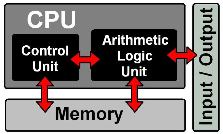
Figure 1: Scheme of the basic parts of a computer [7]. The red arrows indicate information flow.

The data moves to and from the ALU through a memory hierarchy following the pattern displayed in fig. 2.

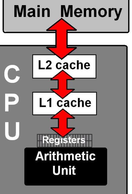
Figure 2: Scheme of the flow of information (red arrows) in a computer to and from its Arithmetic Unit through a hierarchy of memories [7]. The cache can have more levels (not necessarily two). Usually, the closer a device is to the Arithmetic Unit, the faster the information transferring, but the lower the storage capacity (see fig. 3). The disk, as well as eventual external memories like tape libraries, are not directly connected to the CPU. Some architectures also include direct access paths which connect the registers with the main memory.

Information can be stored in numerous devices which exist for that purpose (the memory), each having a different maximum amount of bytes for storage (size) and different bandwidth (maximum rate for information transfer). They also have distinct latencies (the latency is the amount of time between a request to the memory, and the time when its reply takes place). For example, if $y$ bytes of information are to be transferred from a memory device which has a latency of $l$ seconds, and a bandwidth of $b$ bytes/second, then the minimal time required for the information to be delivered will be $t=l+y/b$. Not only do the different kinds of memory have a latency and a bandwidth, but also the network does. Latencies and bandwidths have a major influence on a computer’s performance, especially in parallel machines (see section 4). In fig. 2 we can see the scheme of connection of an arithmetic unit with several types of memories. Commonly, closer connections are with memories with lower latency and higher bandwidth, though smaller size. A scheme of the memory hierarchy, including their present-day typical sizes, bandwidths and latencies, is displayed in fig. 3.

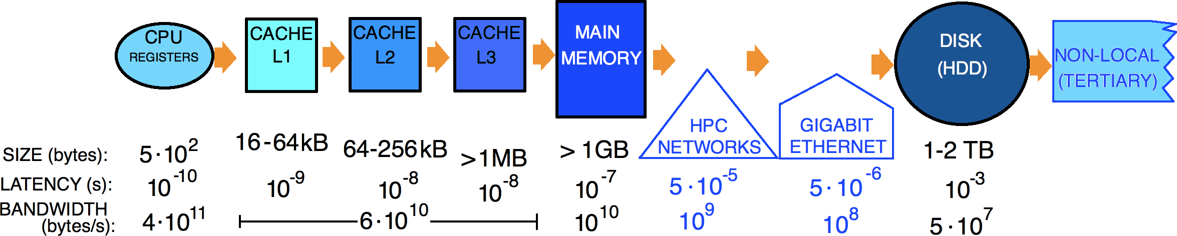
Figure 3: Hierarchy of memories in a computer [7, 9, 10], with typical values of their latency, memory size and bandwidth. The lower the delay in data transfer (latency), the higher the bandwidth and the lower the size of the memory. Blue borders indicate elements typical in supercomputers, while black borders indicate elements which are present both in supercomputers and in personal computers. White shapes do not represent memories, but networking devices for interconnection of nodes in supercomputers.

The information which is expected to be used immediately by the CPU is stored in its registers, which have a very low latency, but can only store a small amount of information. At present, typical CPUs have between 16 and 128 user-visible registers [7]. The next level in the hierarchy of memories (after the registers) is the level of cache memories. Typically, there exist three different levels within this cache memory, which are usually denoted with L1, L2, L3. When the CPU needs some data, it first checks whether or not they are stored in the cache. Efforts in circuit integration are specifically aimed at increasing the storage capabilities of caches, in order to reduce the time to access the information the CPU requires.

After caches, the next level in the memory hierarchy is the main memory (which is sometimes called RAM, although this acronym refers to a specific type of technology).

The disk (hard disk drive, or HDD) has larger storage space, but higher latency and lower bandwidth. Although access to the disk is the slowest if compared to access to other memories, it has much more capability of storing information permanently [11] (external memories, such as CD-ROMs, pen drives, etc. excepted). The first disk memory was developed by IBM in 1956. This first device was able to store 2 kilobits/in², while disks manufactured today can store data at densities of 0.25 Terabits/in² [12]. In the last decades, the space of data volumes is doubling each year or even faster [13, 14]. It is worth mentioning that the increase in disk memory capabilities has been boosted by the discovery of giant magnetoresistance [15, 16]. This phenomenon makes it possible to manufacture MRAM memories which store information (bits) in magnetic layers [17], resulting in storage capabilities larger than those of previous technologies.

The increase in memory size of devices such as caches, RAMs and disks is quite useful for scientific simulation, because much of the information of the tackled complex systems has to be stored frequently during the calculation process, which makes memory an important limiting factor for in silico scientific calculations. Both the amount of available memory (in disk) and the speed to access information in all levels of the hierarchy imply major limitations to scientific calculations. Data storage is reported to be a big energy consumer; moreover, its power intake tends to grow because storage requirements are increasing over and over, and disks are faster and faster [18] . The low speed to access the information on disks is another drawback of the current technology. I/O (input and output to disk) bandwidth has not advanced as much as storage capacity. As stated in [13]: ’In the decade 1995-2005, while capacity has grown more than 100-fold, storage bandwidth has improved only about 10-fold’.

External devices to store information can be considered the last level in the hierarchy of memories. These devices can be CD or DVD disks, USB flash drives, or different technologies. Massive storage devices, such as tape libraries (see fig. 4), are often used in supercomputers. Sometimes, the words primary memory for registers, cache and main memory, secondary memory for hard disks and tertiary memory for non-local memories are used.

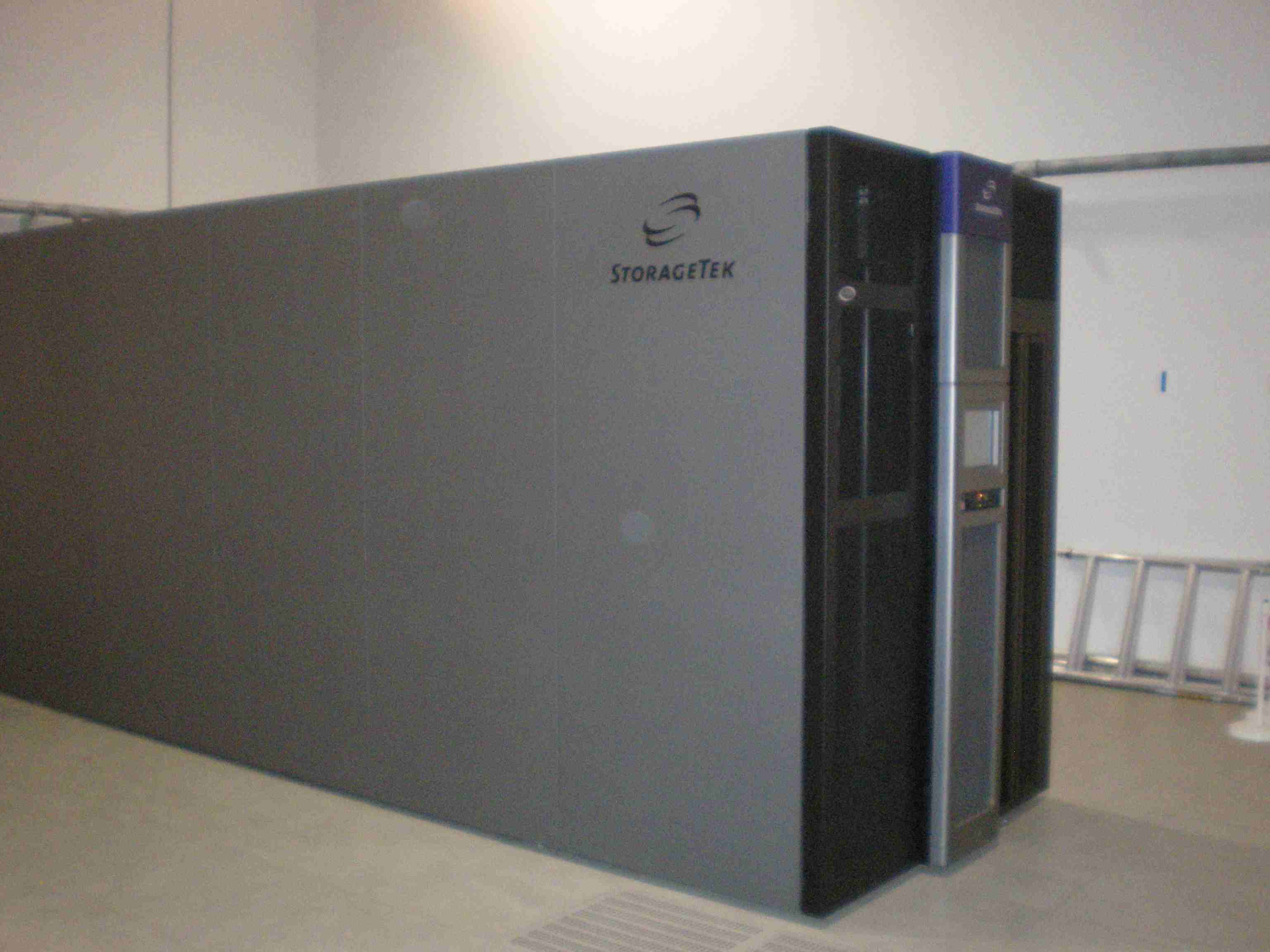
Figure 4: Non-local tape memory at the JSC (Jülich, Germany).

3 Beyond the Von Neumann paradigm

The basic computer scheme of fig. 1 comes from the Von Neumann paradigm [19], which was defined in the early times of computer architecture. This scheme has been kept across time because new designs have been required to work with previous software, which (in the beginning) was devised to be coherent with Von Neumann’s pattern. However, this architecture is not optimal for many present-day purposes, since it is inherently sequential [20]. The CPU can only deal with one instruction with (possibly) a single operand or a group of operands at a time (i.e., at a given clock cycle). Another main drawback is the Von Neumann bottleneck, which results from the fact that data and instructions must be continually provided to the CPU, thus making it inevitable to perform many time-consuming accesses to the memory. Attempts to improve the speed of performing operations continue to be developed. Some of them are related to software techniques and compilers, while others are related to the CPU machinery. Among the latter, we highlight the following ones [7]:

• Integration: Semiconductors research has boosted the miniaturization of transistors, thus enabling an exponential growth of the number of them which can be included on a single chip (see fig. 6). Since the 1960s, the number of transistors that can be included on a semiconductor chip approximately doubles every two years. This fact is known as Moore’s Law [21]. Most transistors on a chip are used to store information in the cache memories. Since the time required to access cache’s information is much lower than that of other memories (see fig. 3), this integration of transistors makes computations faster. Processors released in the years 2008-2011 have typically of the order of $10^{9}$ transistors, and their surface is on the order of squared centimeters. The integration of circuits can increase the performance of all simulations, since the lower the time to access the information to deal with, the lower the total required execution time.

• Clock-rate increase: Until recently, the clock frequency has followed its own ’Moore’s Law’, growing exponentially, although at a lower rate than the number of transistors per chip (increasing about 1.75 times every two years). This growth has recently (c. 2006) collapsed [14] (see fig. 6) because the higher the clock-rate, the larger the power consumption, which scales with the cube of the clock-rate [20, 22], and higher rates would require cumbersome cooling systems. The increase of clock-rate has a direct effect on a computer’s performance, since in principle every operation takes a given number of clock cycles, and reducing the time of every cycle will reduce by the same factor the total execution time. As an example, in fig. 5.A) we present the relation with the inverse of the clock-rate of the total time required to evaluate a self consistent field (SCF) iteration in the calculation of the ground state of a system of five atoms (CH₄). In these tests, the Density Functional Theory (DFT) code Octopus [23, 24, 25] was used in an Intel(R) Core(TM) i5 CPU 750 computer.

• Pipelining: This consists of making different functional parts of the CPU perform different stages of a more complex task. For example, assume an instruction consists of 5 stages, and each has to be performed by a different part of the CPU after the previous stage has been completed. If every stage takes one clock cycle, then to perform the whole instruction would require 5 cycles. But if every part is giving one result per clock cycle, up to 5 instructions could be run every 5 cycles (the optimal performance for pipelining is one instruction per cycle). Splitting instructions into many stages can therefore increase the speed of calculations. Pipelining enables greater clock-rates, although, as stated above, clock-rate is limited by the power consumption. Modern processors are strongly pipelined, and some of them divide basic instructions into over 30 stages.

• Superscalarity: This is the capability of CPUs to provide more than one result per clock cycle. It is essentially based on hardware replication. A superscalar CPU is capable of finding and decoding several instructions per cycle (commonly 3 to 6 nowadays). This can be done because its registers can take information from several levels of the memory hierarchy at a given cycle. In addition, several ALUs do work simultaneously. Superscalarity is also partly based on pipelining. The availability of very fast caches, which can perform over one load or store operation per cycle, also improves superscalarity. The compiler should take advantage of the superscalarity features of a computer.

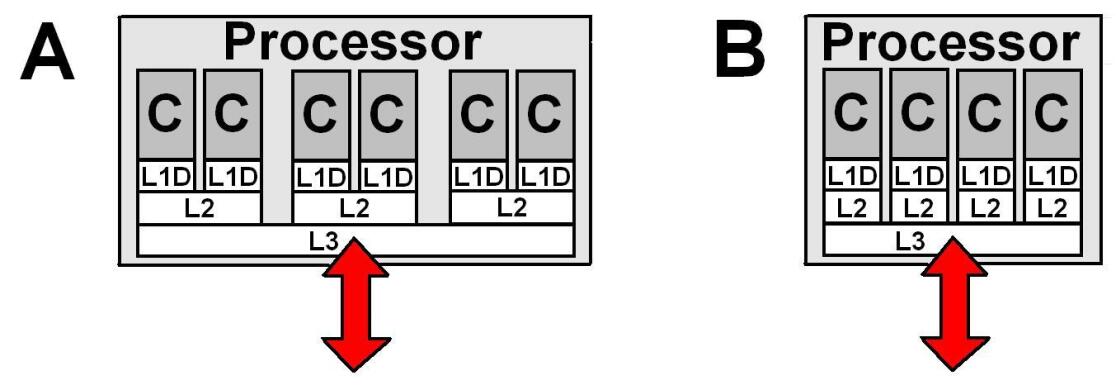
Figure 7: Two possible schemes for a multicore processor. A) Hexa-core processor chip with separate L1 caches, shared L2 caches for pairs of neighboring cores and a shared L3 cache for all cores; B) Quad-core processor chip with separate L1 and L2, but shared L3 cache [7].

• Multicore architecture for processors: In order to overcome the limitations given by the sequential nature of the Von Neumann model, a powerful solution is to include not only one, but several CPUs (cores) per socket, thus forming multicore processors. This new paradigm uses the additional available transistors to put new computation units to work, rather than to try to make a single core faster [14]. Multicore solutions are employed more and more in common PCs. They are also a common solution to circumvent the problem of the high energy consumption in supercomputers [26, 22], since multicore schemes enable the performance of the processor to be increased even if the clock-rate is lowered. The multicore processor architecture shares the increasing available transistors (being doubled every two years according to Moore’s Law) among the cores. The inclusion of more cores, however, also carries some inconveniences. For example, the growth of the number of cores per chip implies a reduction in both the main memory bandwidth and the cache size available for each core. Another inconvenience of multicore architecture is that the presence of many CPUs simultaneously solving the same problem implies that the code of the programs should be devised to provide them with the appropriate parallel instructions, which they should execute at the same time. The recent trend to use multicore processors can be appreciated in fig. 6. It is worth remarking that while pipelining and superscalarity are perfectly compatible with the Von Neumann model, the multicore architecture is not. It is a modification of that paradigm, which entails new rules for the flow of information and the way in which the computer acts on it. The multiple cores of a processor can either lie on the same chip or not, but they lie on the same socket. Some examples of multicore schemes are displayed in fig. 7. Typical PCs have a single socket, while servers commonly contain two to four sockets, all sharing the same main memory. Big parallel computers (see sec. 4) commonly contain many sockets. In fig. 5.B) we present an example of how increasing the number of cores reduces the total time for a given task. The task of this example is the calculation of a SCF iteration in the calculation of the ground state of a system of 180 atoms using DFT. For this calculation, the Octopus [23, 24, 25] code was used in the Jugene (IBM Blue Gene architecture) cluster.

  

  

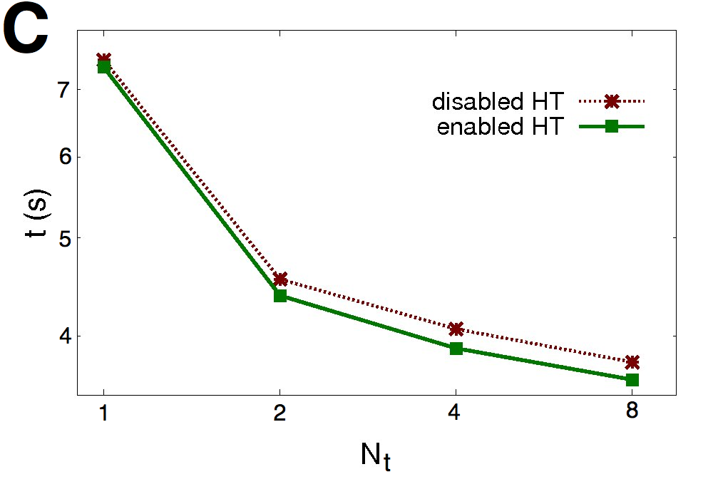
  Figure 5: Average time (t) required to calculate: A) one DFT-SCF iteration in the calculation of the ground state of a system of five atoms (CH₄), as a function of the inverse of the clock-rate (r^-1); B) one DFT-SCF iteration in the calculation of the ground state of a system of 180 atoms (chlorophyll), as a function of the number of cores taking part in it (N_c); C) the electrostatic potential created by a Gaussian charge distribution as a function of the number of threads (N_t), with the Hyperthreading option disabled and enabled.

• Multithreading: This is the ability of a core to execute instructions corresponding to several threads (several execution lines) which can be run in parallel (doing operations in different ALUs) or sequentially. These threads can either be independent or mutually dependent. Multithreading is possible because a core has several sets of registers, each set storing information of a given thread, although all threads in a core share common caches and depend on a single Control Unit. Multithreading is complementary to multicore architecture, since both parallelize the execution at distinct levels. In fig. 5.C) we show an example on the execution time of the influence of using Hyperthreading (a concrete type of Multithreading). The example corresponds to the calculation of the electrostatic potential created by a Gaussian charge distribution represented in a real space grid, and was run with the Octopus code in an Intel(R) Core(TM) i7-2600 CPU @ 3.40GHz machine. Note that this example is just qualitative: the increase of performance of multithreading strongly depends on the concrete problem and on how the software to tackle such problem is devised.

• SIMD instructions: SIMD (single instruction multiple data) instructions enable data parallelism by performing arithmetic operations not on a single number, but on a vector of them. The supercomputers of the 1980s and early 1990s were based on this principle (although at a much larger scale) and they were called vector machines. Although big vector machines are rare at present, its principle is still useful for other computers (e.g., multimedia instructions are used for most general purpose present-day processors). The use of SIMD instructions has proven to increase the performance of simulations in many fields such as, for example, molecular dynamics, fluid dynamics [27] or astronomy [28]. For example Machines using GPUs instead of CPUs (thus executing the same instruction on many data simultaneously) typically increase their performance in over one order of magnitude [29] in molecular dynamics simulations. Computers not using GPUs can also take advantage of the SIMD paradigm, since more and more often they use registers of bigger size (say 128 bits vs 32 bits), which enables an ALU to do the same operation on various input variables simultaneously. The possibility to do this strongly depends on the software and the compiler, for the CPU must ”guess” when (in what loop of the code) this can be done. An example of software developed to take advantage in the SIMD paradigm in molecular dynamics calculations is NAMD, where increasing factors of 2 to 4 in the performance are common [30]. Even for non-SIMD optimized programs, SIMD can result in an increase of performance. For example, the average value of the time required for a SCF iteration in the calculation of the ground state of CH₄ (i.e., the example pointed when the clock-rate was discussed) is about a 5% longer if SIMD are disabled.

• Out-of-order execution: If the arguments of the instructions are not available in registers when they must be used (this can happen if the memory is too slow to keep up with processor speed) out-of-order execution can prevent computing units from being idle.

• Simplified instruction sets: Paradigms of instructions sets which are rather simple (as opposed to previous models) but can be executed much more quickly. The RISC (Reduced Instruction Set Computer) paradigm was adopted during the eighties, resulting in efficiency increases.

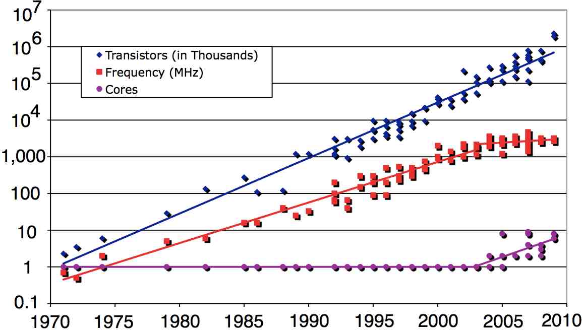
Figure 6: Evolution in time of the number of transistors per chip (blue), clock-rate (red) and number of cores per processor (purple). It can be appreciated that during the last years the clock-rate has collapsed, while multicore solutions have started to be implemented. The number of transistors continues to grow exponentially at a steady rate, satisfying Moore’s Law to be still satisfied (Courtesy J. Dongarra; data from [20]).

All these improvements can be useful for simulation in essentially all the fields of Physics, because they are quite general. The specific problem and the software to tackle it will determine the point the increase in performance reaches.

The trends in the evolution of the degree of integration of processors, their clock-rates and their numbers of cores are displayed in fig. 6. We could say that the time of steady growth of single-processor performance seems to be over [14], which has spurred the semiconductor industry to start a transition from sequential to parallel computers. The introduction of multicore processors in 2004 (see purple line in fig. 6) marked the end of a 30-year period during which sequential computer performance increased from 40% to 50% yearly. The trends displayed in fig. 6 have lead to a reinterpretation of Moore’s Law. In words of Jack Dongarra (coordinator of the top500 project): ’The number of cores per chip doubles every 2 years, while clock speed decreases (not increases). The number of threads of execution doubles every 2 years’. This increase in the number of threads results from both the multi-core solutions and from the hardware modifications which enable CPUs to work on other tasks when one executing thread is stalled (for example, waiting for data) [11]. These capabilities increase computer performance, but require the software to be well suited to the hardware to reach maximum performance. Although in the next years eventual physical limitations for technologies might make the thread increase trend stop, important advances are being achieved in the direction of core integration. Intel has recently presented a prototype research chip which implements 80 simple cores, each containing two programmable floating-point engines. This is the maximum single chip integration to date, and reaches TFLOPS performance [3].

4 Parallel computers

As stated above, the idea behind most powerful computers nowadays is the use of many cores (which globally contain many CPUs). A given program is divided into several execution lines (threads) which are simultaneously run in the different cores. Therefore, these cores solve the problem in a cooperative way. The number of cores used by a supercomputer is continuously increasing in time. As stated above, the definition of ’supercomputer’ or ’high performance computer’ is rather arbitrary, because these expressions refer to computers which are much more powerful than common computers. Because of the technological advances, it is said that today’s supercomputers are tomorrow’s PCs (see fig. 15; since a present-day laptop is capable of doing about $10^{10}$ operations per second (10 GFLOPS), it is as powerful as a supercomputer was 14 years ago). The use of standard computer components to build supercomputers (the so-called commodity clusters) has made these high performance machines accessible for many research groups throughout the world.

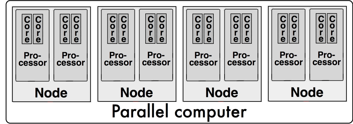
Figure 8: Scheme of a parallel computer. It can be divided into four levels (core, processor, node and parallel computer itself). Each core contains a CPU, the basic computing unit.

We call a parallel computer a collection of connected cores lying in different nodes, which are connected by networks. The cores of an operating parallel computer work simultaneously in a cooperative manner. A parallel computer is formed following a scheme such as the one displayed in fig. 8. It can be decomposed into four levels: cores, processors, nodes and the parallel computer itself. Components inside a given level have distinct features (e.g., bandwidth, latency, etc.) when communicating with other components inside or outside its own module (e.g., a core communicating with one core in the same processor will do it much more rapidly than with a core lying in other processor). We can summarize the four levels of a parallel computer as follows:

• Core: It contains one Control Unit, and one or several arithmetic-logic units (and therefore one CPU). For example, cores devised under the Intel Core microarchitecture have three ALUs [31]. A core can run one or several execution threads simultaneously.

• Processor: Integrated circuit which contains one or several cores and is lying on one semiconductor layer (chip). One or several processors are inserted in one socket.

• Node: Set of processors which share a common main memory, and commonly also share other resources, such as a hard disk drive or a network connection. It usually consists of one motherboard where there are several sockets. Communication among processors in a given node is rather fast, and is provided by buses.

• Parallel computer: It comprises all nodes and the communications among them, which are provided by networks such as Infiniband or Gigabit Ethernet.

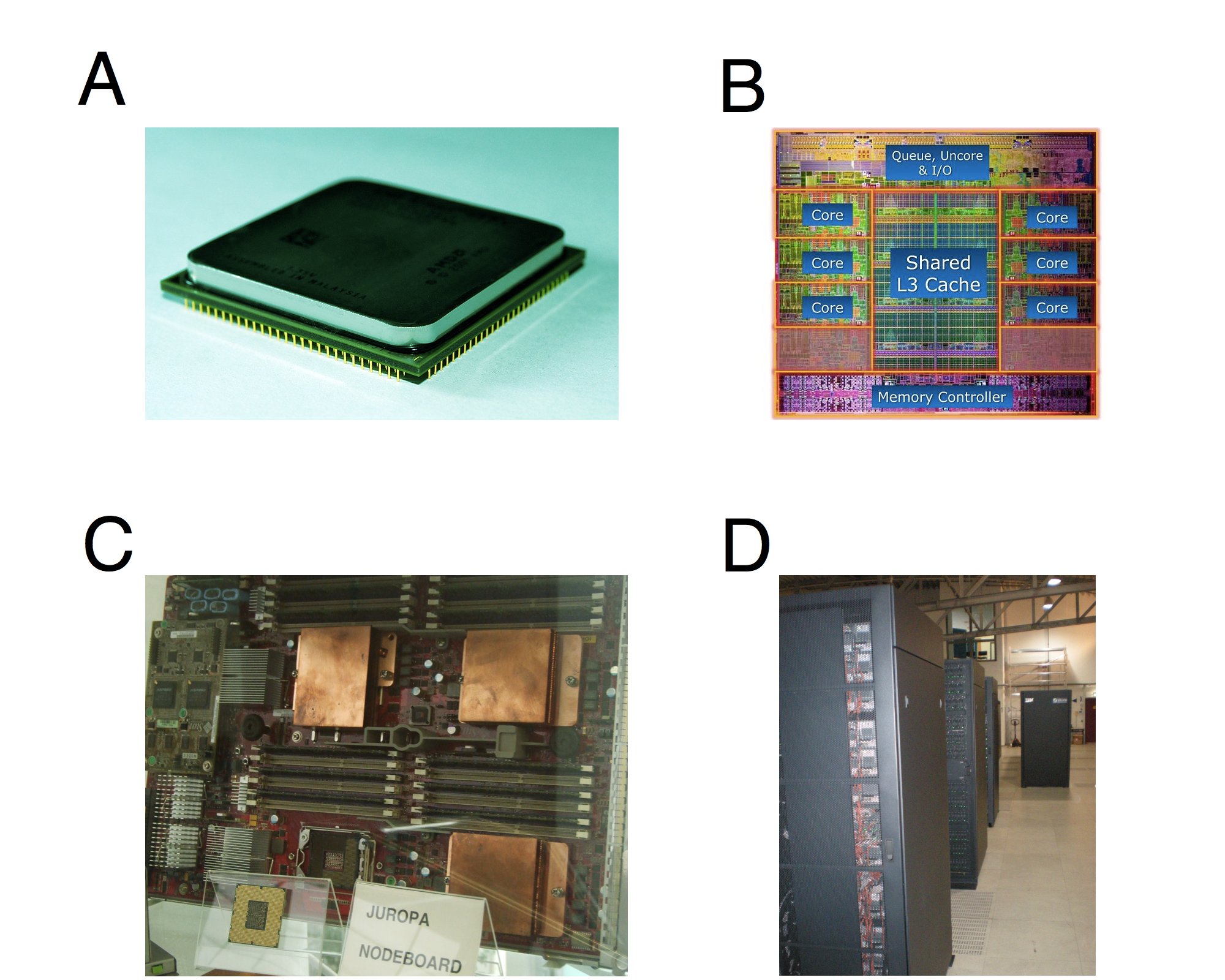
Figure 9: Examples of the constituents of a typical parallel computer. A) Processor (Dual-Core Athlon 64x2 - 6400plus); B) Inner scheme of a processor (Intel Core i7-3960X Extreme Edition 6-core processor); C) Node (the image shows the motherboard of a node of the Juropa cluster at the JSC, lacking the hard disk); D) Cluster (the image shows parallel computers at the JSC, Jülich, Germany). Image C) courtesy J. Alberdi. Image A) Copyright (c) 2011 Pablo García Risueño. Permission is granted to copy, distribute and/or modify this image under the terms of the GNU Free Documentation License, Version 1.2 or any later version published by the Free Software Foundation; with no Invariant Sections, no Front-Cover Texts, and no Back-Cover Texts. A copy of the license can be found in http://www.gnu.org/licenses/fdl-1.2.html.

In fig. 9, images corresponding to the different levels enumerated above are displayed. A) displays a processor, which contains two cores (each containing several control and arithmetic-logic units). B) displays the scheme of a 6-core processor. A motherboard (C), together with devices joined to it, form a node. Several nodes linked by interconnection networks form a parallel computer (D).

Networks connecting the constituents of a parallel computer have a critical importance for the parallel performance of applications in it. This is because data transfer typically is the dominant performance-limiting factor in scientific code [7]. The most important network characteristics that need to be taken into account in order to produce efficient parallel code are its network topology (the way the nodes are connected) and its network bandwidth and latency (see fig. 3). These features have an important influence on the performance of the parallel computer. Examples of common topologies are ring, grid, torus in 2 or 3 dimensions or tree [11].

We will now briefly describe various types of existing parallel supercomputers. We will first introduce the essentials of parallel computers, and then some fundamentals of other devices, like GPUs, special-purpose computers and heterogeneous computers, and of other types of computation, like the cloud computing and grid computing.

Parallel computers are commonly classified into two paradigms: shared-memory and distributed memory. The latter are also known as clusters. Both operate under the MIMD paradigm, i.e., multiple instructions are given to multiple cores, which deal with multiple input variables (data). Other systems, like GPUs, vector machines or some microprocessors follow the SIMD paradigm (see sec. 2), and they execute a single instruction on a set of multiple data.

A shared-memory parallel computer is defined [7] as a system in which a number of CPUs operate in a common shared physical address space. Important versions of this paradigm are:

• UMA (uniform memory access): The access time of all processors for the main memory is (essentially) the same. This is attained with communication devices having the same latency and bandwidth.

• ccNUMA (cache-coherent Non-uniform Memory Access): The main memory is physically distributed across the various processors, but the circuits (logics) of the machine make this set of main memories to appear as only one large memory, so the access to different parts is done using global memory addresses. The access time is different for different processors and different parts of the memory, as in a distributed-memory computer.

The scheme of the UMA paradigm can be found in fig. 10. In UMA architectures, a device called chipset controls the information flow between the main memory and the cores. The simplest example of UMA is the dual core machinery that recently has become very popular [3]. The complexity of the circuits required to keep the access time uniform, at present, limits the largest UMA systems with scalable bandwidth (the NEC SX-9 vector nodes) to sixteen sockets [7].

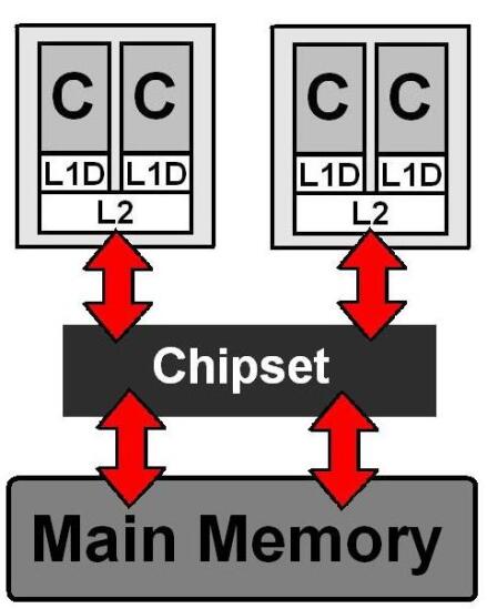
Figure 10: Scheme of a shared-memory UMA machine consisting of two dual-core processors [7].

Typical patterns of shared-memory ccNUMA machines are displayed in figures 11 and 12. A ccNUMA computer consists of several local domains, whose memories are locally connected (each local domain being basically a UMA). The memories of different local domains communicate via so called coherent links. This architecture is appropriate for large shared-memory machines, but is more often used to build small 2- or 4-socket nodes in supercomputers.

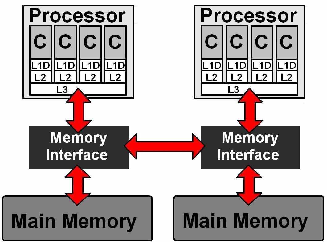
Figure 11: Pattern of a ccNUMA system with two locality domains and eight cores. Red arrows indicate information flow. The information is managed by a memory interface. Memory interfaces are connected via coherent links (for example, the central red arrow in this picture) [7].

An architecture which is more widely used to build large supercomputers (up to thousands of cores) is the one whose scheme appears in fig. 12. Each processor socket is connected to a communication interface (S), which provides memory access to the proprietary NUMALink network. The NUMALink network uses routers (R) for connections with nonlocal units. The asymmetry of this design makes the access times very variable for different processors and different memory positions. ccNUMA machines also have the drawback that two or more different processors may try to access the information at a given memory position simultaneously, and thus they would compete for its resources. In addition, the input/output human interface is connected with only one local domain.

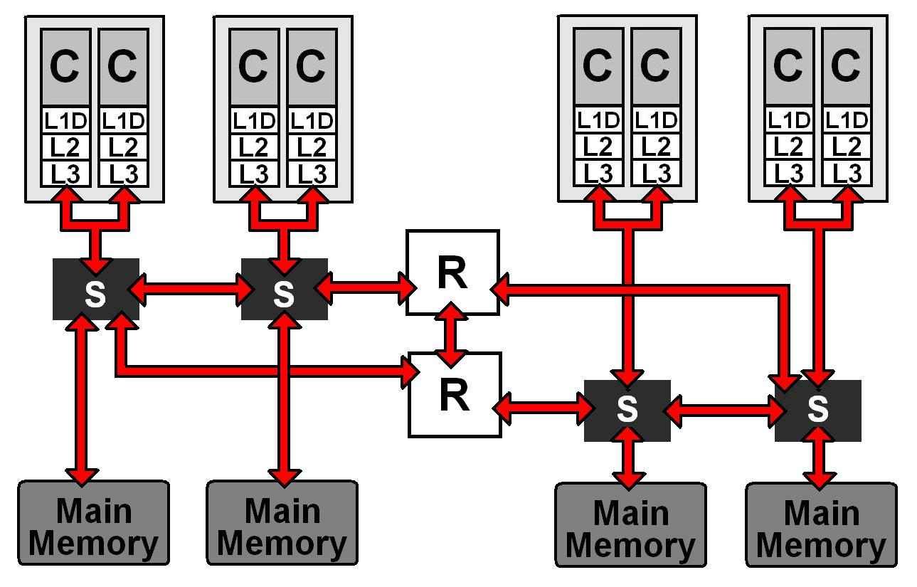
Figure 12: A ccNUMA system with four locality domains, each comprising one socket with two cores. Each socket is linked to a communication interface S, and the traffic of information is managed by some routers R [7].

Pure distributed-memory computer schemes would include one main memory per core, each being connected to all or part of the others. Such patterns, however, are seldom found because of their price/performance features. Most of the so-called distributed-memory machines (which are indeed a large portion of supercomputers) are actually hybrid models, i.e., distributed-memory machines whose building blocks (nodes) are shared-memory-like devices [11].

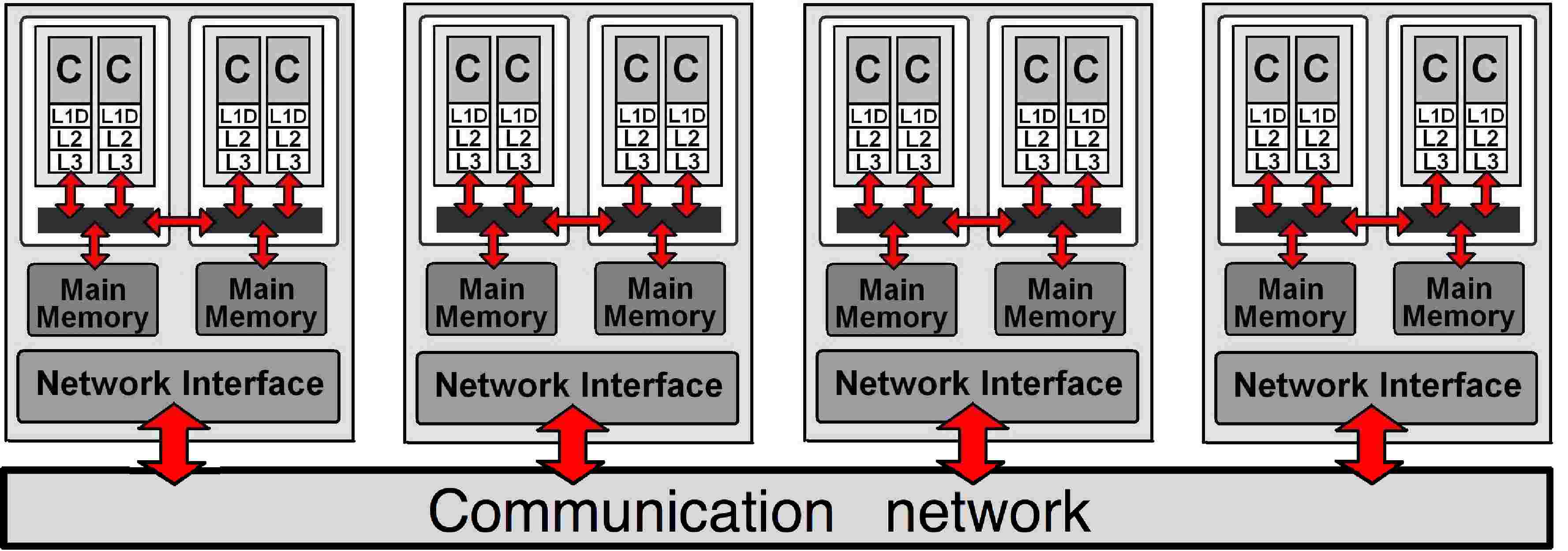
Figure 13: Pattern of a distributed-memory computer. Red lines indicate information flow [7].

When the code being executed at a given core requires information which is stored in the memory belonging to another node or in another disk memory location, the core must send a request for that information. The request reaches the core after travelling through the network connecting the parts of the cluster.

For supercomputation purposes, these connections were in the past made with the Gigabit Ethernet technology (see fig. 3). At present Infiniband has become very popular (see fig. 17). It is worth stressing that at present there exist serious inconveniences with information transfer devices, because they transfer information much slower than standard CPUs perform operations. For example, Infiniband connections have a latency of the order of microseconds ($10^{-6}$ s). Since present-day clock-rates are of the order of GHz, and a floating-point operation takes of the order of tens of clock cycles, a typical operation can take about $10^{-9}\sim 10^{-8}$ s. Therefore, transferring the information of the result of an operation between nodes will be at least 100 times slower than performing the operation. In addition to latency, the bandwidth of the network can also be a limiting factor. Delays produced by nonzero latency and finite bandwidth are the reasons why minimal feedback among different nodes is pursued by algorithm developers [32]. Feedback among cores with fast connections, such as those belonging to the same processors, need not usually be avoided [20]. It is said that, qualitatively, the speed of a serial computer is determined by the caches, while the speed of a parallel computer is especially determined by the speed of communications among nodes [33]. Standard values of latencies and bandwidths of caches and networks can be viewed in fig. 3. There exist some ways to compensate for the big difference of latency between caches and networks, like the communication latency hiding, that consists of overlapping communication with computation (or with other communication) [33].

The dominant HPC architectures at present and for the foreseeable future are comprised of nodes which are (shared-memory) NUMA machines themselves, and which are connected with the rest of the nodes following a distributed-memory pattern [8]. A popular architecture of distributed-memory computers is IBM’s Blue Gene (see fig. 14). In Blue Gene [34], processors lie in the vertices of a cubic grid. Each processor communicates with its six nearest neighbours in a 3D torus topology (the last processor, in the border of the grid, is linked with the first one, in all three directions).

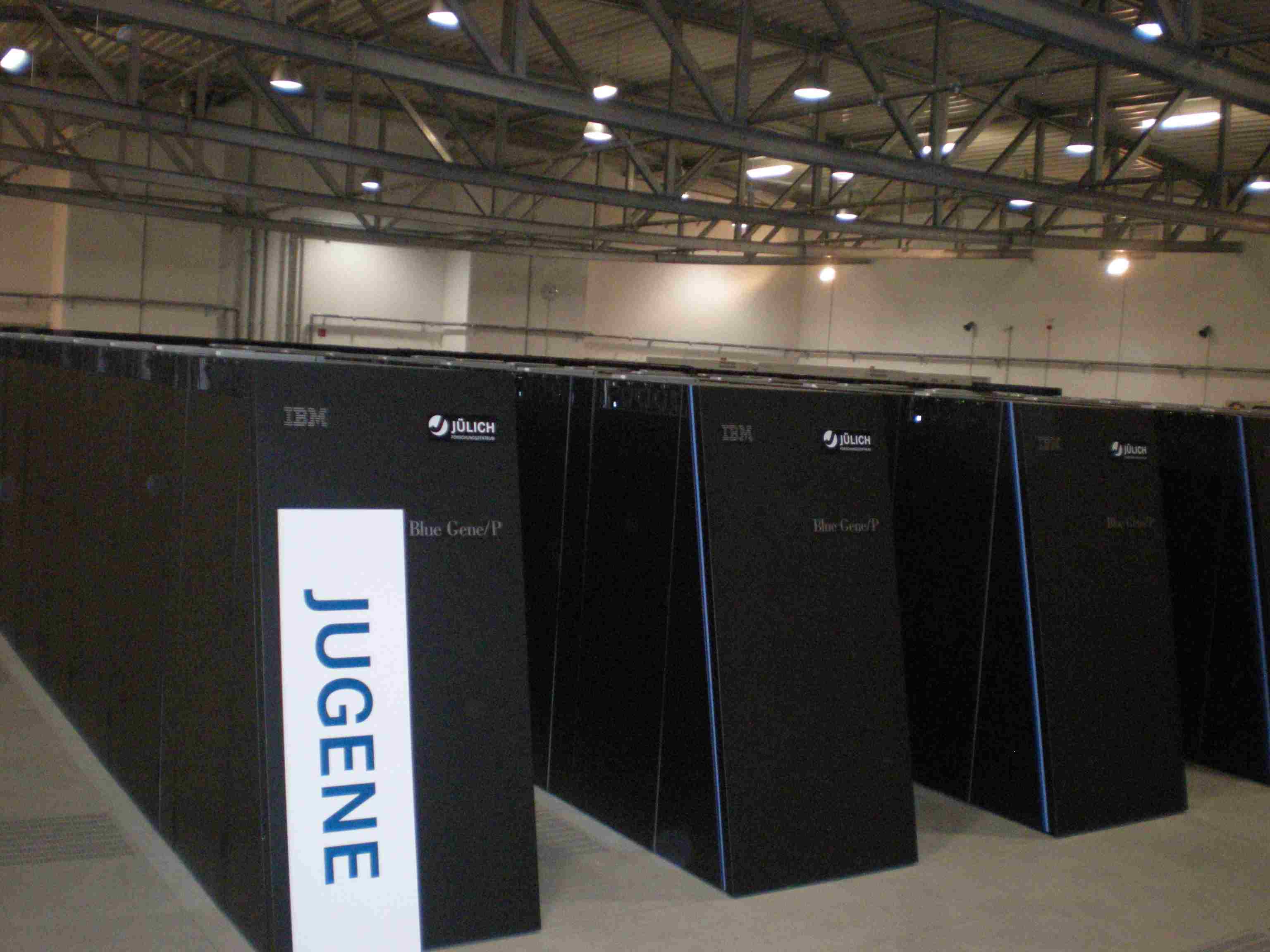
Figure 14: The cluster supercomputer Jugene (IBM Blue Gene / P technology), in the JSC (Jülich, Germany) in Sept. 2010. In that moment, it consisted of 294,912 cores, what made it the most powerful computer in Europe, and the fifth most powerful computer in the world.

If a problem is to be solved in a cooperative manner by the various cores of a cluster, the code to be executed must be written so that the workload is shared among them. The MPI (Message Passing Interface) protocol [35] is appropriate for writing codes that run in parallel in distributed-memory machines, as well as for shared-memory machines. The increasing popularity of MPI at present comes from its simplicity and its availability of standard libraries. The parallelizations of many Physics and Chemistry simulation programs are based on MPI, although other parallelization paradigms are also used [11]. Despite its remarkable advantages, the MPI paradigm has an important drawback. Information transfer between two parallel threads requires both of them to reach a synchronization, i.e., one must execute the instruction for sending information (MPI_SEND) and the other one must execute the instruction for receiving it (MPI_RECV). In this way, the sender core will be idle until its information is be received. The limitations of the MPI scheme can be overcome by providing facilities for a process to access data of another process without that process’ direct participation [11]. Performance in shared-memory machines can be increased by using the OpenMP interface. Since most supercomputers have hybrid shared-distributed-memory architectures, mixed use of different programming codes, including both MPI and OpenMP is advisable [8]. However, many programmers use only MPI, for the sake of simplicity in their codes.

5 Hybrid and heterogeneous models

A supercomputer can either be formed by the repetition of processors of the same kind, or by different ones, such as general purpose processors, graphics processing units or special-purpose chips, among others. In the former case, the architecture is called homogeneous, while in the latter case, it is called heterogeneous [36]. Heterogeneous machines can have advantages with respect to homogeneous machines in power consumption, efficiency of data transfer and parallel speedup. The Cray supercomputers are examples of heterogeneous machines, which get high performance by using different kinds of processors within the same cluster computer.

Using graphics processing units (GPUs [37]) as a part of (heterogeneous) clusters is a more and more popular solution. GPUs were originally devised to perform fast calculations on data for creating images. However, in recent times, they have become celebrated in the context of supercomputing. This is because they are capable of treating large amounts of data (vectors of data, rather than single variables) simultaneously. A GPU can perform some given tasks several orders of magnitude faster than a CPU. For example, in some problems of data analysis, GPUs performance can gain about a factor of 200 with respect to CPUs performance. For general-purpose computation issues, GPUs can either be included in motherboards together with CPUs, or different types of devices (GPGPUs [26]) can be produced that can work without a CPU. Full clusters can be built on GPGPUs instead of CPUs. As a sign of the current success of GPU-based solutions, it can be noted that four out of the ten most powerful supercomputers (in the list of top500 as of June 2011) include GPUs.

A different kind of supercomputing facility is the one formed by the special-purpose computers. These machines cannot deal with a very broad range of different tasks, as the general-purpose computers (PCs, laptops, most supercomputers, etc.) can. Instead, they are devised to execute a limited set of algorithms, but with great efficiency. An example of a special-purpose computer is Anton, which is dedicated to protein molecular dynamics. Anton was able to run a simulation corresponding to 1 ms (in a huge number of steps, since $\Delta t$ is of the order of fs in proteins), realizing the hard task of predicting the folding of a protein [38, 39]. Other examples of special-purpose computers are Janus [40], which is used for simulation of spin glasses, and GRAPE-6 [41], for astronomy.

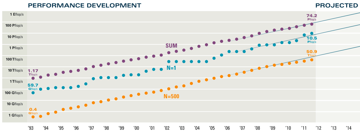
Figure 15: Evolution of computational capabilities: purple line: Aggregated power of all 500 most powerful computers in the world, according to the top500 list; blue line: most powerful computer in the world, according to the top500 list; orange line: 500th most powerful computer in the world. Notice that the vertical axis is logarithmic. Source: top500 (www.top500.org).

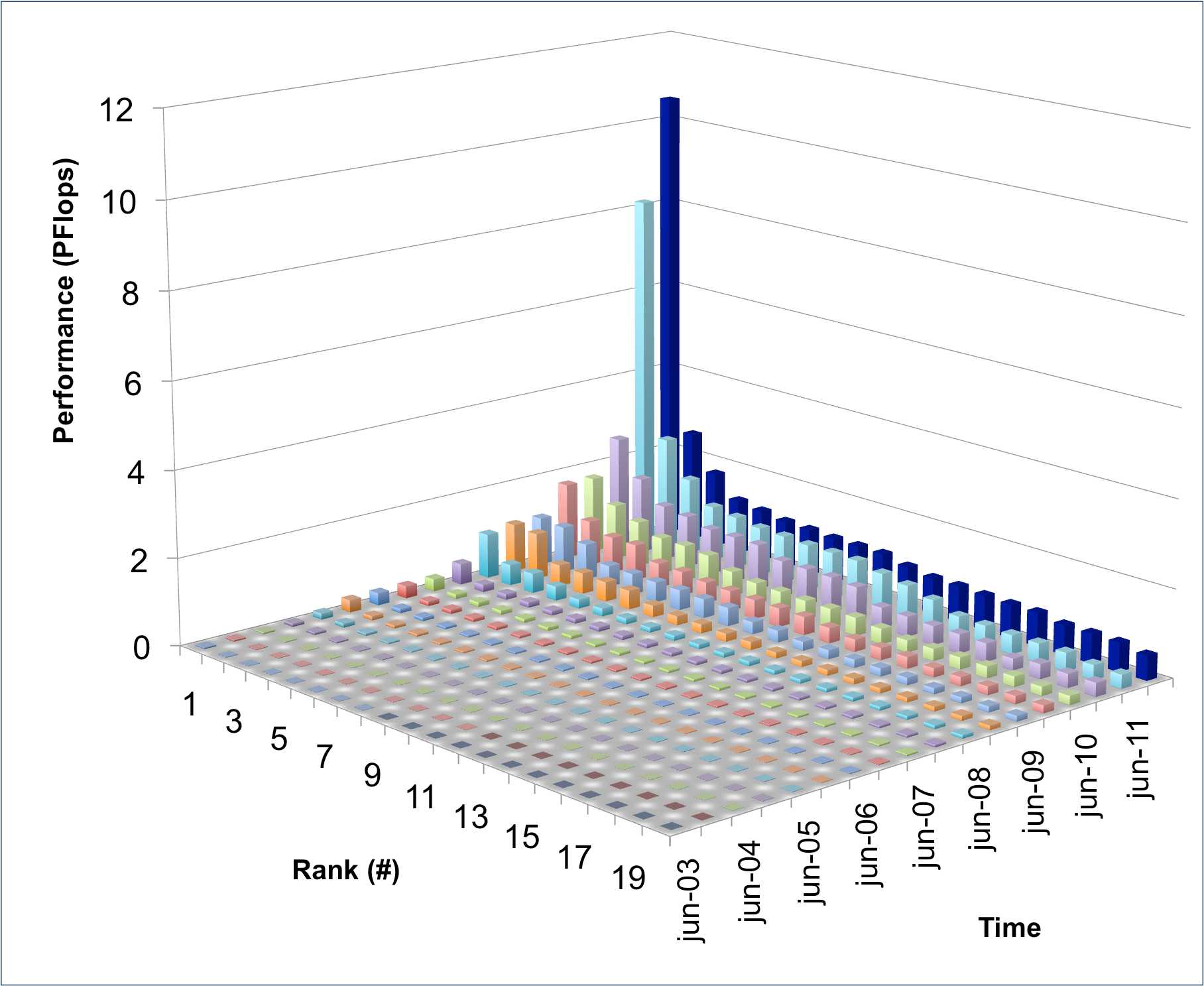
Figure 16: Evolution of the performance of the twenty most powerful computers on the world from June 2003 to November 2011. (Source: top500 —$R_{max}$—).

Fig. 6 and some of the subjects discussed so far can give us an idea of the evolution of computational capabilities of modern computers, which grow very rapidly, in an exponential way. In order to quantify this evolution, twice a year a list of the 500 most powerful computers on the world, the top500 list, is released. In order to measure the performance of computers, a benchmark (the HPLINPACK benchmark [42]) is run. The essential task of the HPLINPACK benchmarks is to solve a linear system of equations $Ax=b$ whose coordinate matrix $A$ is dense (i.e., contains no null entries) with partial pivoting. Performance is measured in number of floating-point operations per second (FLOPS) that the machine is able to perform. It is worth remarking that special-purpose computers can hardly appear on the top500 list, because it is essential to run the HPLINPACK benchmark, and many special-purpose computers are not capable of doing it. In fig. 15 we can appreciate the exponential increase of supercomputing performance of the machines in the top500 list, both for individual supercomputers (the most powerful one, and the one in the 500 position, appearing in the figure) and for the aggregated power of all computers on the list. From 1993 to 2011, the combined computing power of the collection of all 500 most powerful computers in the world followed its own ’Moore’s Law’, since it increased about 1.9 times per year (almost twice as fast as the increase in integration predicted by Moore’s Law). By comparing charts 6 and 15, we can appreciate that the trends in chip integration, clock-rate and number of cores per processor and the power of high-performance computers are closely related. In fig. 16, we can see the evolution of the 20 most powerful computers during the last decade. The vertical axis of this graph is not logarithmic, so the dramatic increase can be noticed in a clearer manner. In fig. 17, some features of the top500 computers are summarized. Chart A shows the number of cores high-performance computers consist of. Chart B quantifies something we mentioned earlier in this section, that vector computers are no longer popular, and most modern computers are scalar (i.e., every CPU deals with a scalar variable at a time, not with a vector containing many values simultaneously). Chart C gives an idea of the computer power distributed by countries. Finally, chart D gives a notion on the network communication devices which are used by most powerful supercomputers.

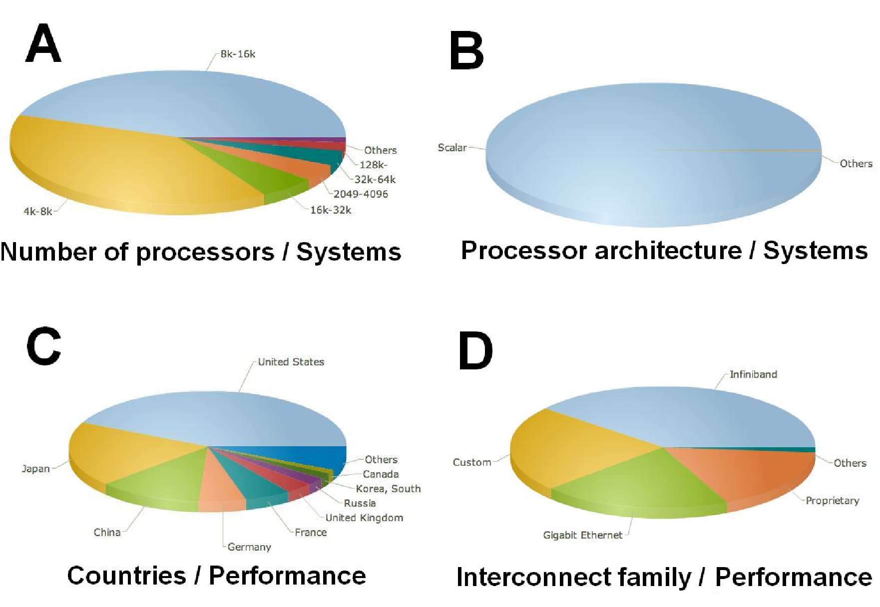
Figure 17: Some features of the most powerful computers in the world, according to the top500 list of June 2011. The data labeled as ’systems’ (upper row) means that every computer on the list enters the charts with weight 1. The data labeled as ’performance’ (lower row) means that the weight depends on the computer’s performance. A: Number of processors; B: Processor architecture; C: Location of machines; D: Family of interconnect devices. (Source: www.top500.org).

The enhanced capabilities of current supercomputers to perform operations very rapidly is very useful for scientific calculations. Most modern algorithms and codes are based on repetition to take advantage of these capabilities. However, developing software for massively parallel machines is harder than for the traditional sequential computers. This is because instructions should be provided to many units working simultaneously, and efficient information feedback among them needs to be implemented. The growing complexity of computers, where many (not necessarily equal) processing units are linked among them and also linked to a hierarchy of memories, each having a different access time, makes parallel programming a rather complicated task. The complexity of computers’ architecture is an extra obstacle for the programmers [20]. More complex internal behaviour of cores, including effects of pipelining and superscalarity makes code execution harder to comprehend in depth and their logic hinders parallelization, because human programmers find it hard to devise codes which are well-suited for these architectures. For example, the programmer can think that the code he writes is executed sequentially and in order in a core, but this is no longer true (as stated when the Out-of-order execution was explained). Programmers are helped by modern compilers, which include several levels of optimization, which can do more efficient mapping in data transfer and result in large efficiency improvements. In order to devise more efficient software codes, tracing and profiling software tools can be very useful [43]. Moore’s Law is said to have enabled cheaper (more efficient) execution of programs, but at a higher cost of developing new programs, by reason of the increasing complexity of computers [14]. In words of J. Dongarra, ’For the last decade or more, the research investment strategy has been overwhelmingly biased in favor of hardware. This strategy needs to be rebalanced, since barriers to progress are increasingly on the software side. Moreover, the return on investment is more favorable to software. Hardware has a half-life measured in years, while software has a half-life measured in decades. Unfortunately, we don’t have a Moore’s Law for software, algorithms and applications’. This does not mean that the aim of efficient algorithms has not been successful, but means that modern algorithms and programs should be well-suited to current machine component features and computer architectures (an example of this adaptation can be found in [3], where the efficiency is increased by means of optimizations of the transfer of data). Indeed, smart software parallelization schemes, including new paradigms, can be the only tool to improve supercomputers’ performance when hardware capabilities no longer increase [20].

A few years ago, machines supporting High Performance Computing have had to face an important obstacle: the significant rise of power consumption. The increase of clock-rates has boosted power dissipation [7], because the power consumed by a core scales with the cube of its clock-rate [22]. This is attributable to the fact that the power is proportional to the square of the voltage multiplied by the frequency, but the voltage itself is proportional to the clock frequency. Power dissipation generates heat, which is an important drawback because semiconductor materials in computers require rather low temperatures in order to work properly. To this end, cooling systems must be implemented. Computers in the 1980s did not need heat sinks; the heat sinks used in the nineties were of moderate size; today’s cooling systems are very big. In PCs and laptops air cooling systems (fans) are usually enough, but in supercomputers water-based cooling systems may be mandatory in a nearby future [20]. The work of cooling systems entails serious power consumption which must be added to that resulting from the processors’ work. As a result of these high power needs, the budget for electrical energy of the computing facilities of a research group may easily be exceeded. As an example [44], a 16-core processor with every core consuming an average of 20 Watts will lead to 320 Watts total power when all cores are active, which will have a non-negligible economic cost. Another example is given by Amazon.com [45]. The energy bill of its data centers costs about the 42% of the total budget of the center (the cooling system consuming more energy than the operation of CPUs). Many ways to reduce the impact of excessive power consumption are being proposed [46, 47]. Architectures for many core machines should be carefully devised to minimize it. A possible solution is to simplify processor designs. Using larger caches is another option, although there is a limit beyond which a larger cache will not pay off any more in terms of performance, due to bandwidth limitations. Multicore processors are the solution which most present computer manufacturers prefer [7].

6 Distributed computing

Data on the top500 refers to well localized large supercomputers (like the one displayed in fig. 14). However, in recent times, other solutions for HPC, such as grid computing, cloud computing and volunteer computing, have become very popular. These three more modern ways of computing are said to be ways of distributed computing. Distributed computing is based on the concept of doing high performance calculations using geographically distant machines, which has been enabled with the advent of the internet and high-speed networks. Computers participating in a given problem can lie thousands of kilometers away from each other, but they can share information through the internet.

grid computing [48] uses geographically distant nodes to solve a given problem simultaneously in a cooperative way. grid computing capabilities are usually managed by a given organization, and the computational resources (mediated by physical machinery) which support the calculations are provided by different supporting institutions and organizations, which can be companies, research groups, laboratories, universities, etc. A management committee distributes the computational capabilities at every moment among the requests of different groups of users. The groups of people taking part in grid computing projects for solving problems are usually called virtual organizations since these groups are frequently heterogeneous, being formed by many people from different organizations which are geographically distributed. The essential aspect of a virtual organization is that it is formed for a specific project. Virtual organizations can act either as producers or consumers of resources (or both). Various virtual organizations involved in a grid computing project are mutually accountable; i.e., if one misbehaves, the others can cease sharing resources with it. Since many computer cores throughout the world are working together, much computing power can be accumulated, which enables solving many problems whose solution may not be feasible even in the most powerful supercomputing clusters. This generates vast amounts of data, which spurs the creation of large collective databases [13]. Large grid computer facilities are often used by a large number of users, which helps to match the demand of the computational resources with their availability.

It is also worth noticing that grid computing projects commonly operate under open-source software standards, which eases the development of software applications and the cooperation among groups. A popular software package to manage grids is the Globus Toolkit, including the GRAM software as a tool for the users. Grid facilities, as well as cluster computers, frequently run in Linux operating systems.

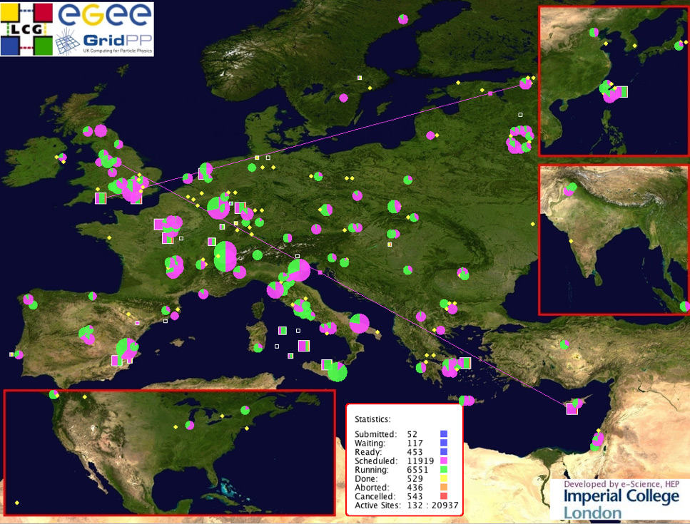
Figure 18: A scheme of geographical distribution of computing nodes of the egee grid (http://www.eu-egee.org). Current grid computing projects often involve facilities in many countries.

grid computing has been successful in numerous research fields, such as drug design, biomolecular simulation, engineering and computation for industry, Chemistry, Geology (e.g. earthquake simulations) or meteorology [48, 49]. It also plays an important role in Particle Physics. For example, the Large Hadron Collider of the CERN sends huge amounts of experimental data to its associated grid facility (the Worldwide LHC Computing Grid, WLCG), so that many scientific groups throughout the world can analyse the data. WLCG involves over 140 computing centres in 35 countries, and includes several national and international grid projects.

Recently, another kind of distributed computing, volunteer computing, has become a useful tool for scientific purposes. volunteer computing consists of using the computation power of machines which were neither devised nor purchased to do scientific calculations, but for use in daily life. Common PCs and laptops connected to the internet, like those in millions of homes, can perform calculations to solve scientific problems. It is only necessary that the owner of the computer agrees and installs the appropriate software (this is the reason why this kind of computing is called volunteer computing). As stated in [32], there are hundreds of millions of idle PCs potentially available for use every moment, and the majority of them are strongly underused. Moreover, while the complexity and the network efficiency have increased following their own Moore’s Laws, the number of computer users has increased at even a higher rate during the last decades, which makes the potential capabilities of volunteer computing huge [32]. volunteer computing has produced many remarkable scientific results in the last decade [50]. Some examples of volunteer computing are the Ibercivis project, seti@home —for the search of extraterrestrial intelligent life— and folding@home[51] —for statistical calculations of molecular dynamics trajectories for models of biological systems—. The last one is a particularly good example of how important scientific results can be produced with volunteer computing for problems which are unaffordable for other HPC schemes [32]. Volunteer computing projects often rely on the BOINC open-source software, which is also appropriate for grid computing. Although grid computing and volunteer computing share some features, there is a key difference between them. grid computing is commonly symmetric while volunteer computing is commonly asymmetric. This is, in the former, one organization can borrow resources one day, and supply them the next; in the latter, contributors (particular computer owners) commonly just provide resources to the project.

Distributed computing has become a powerful research tool because of its numerous advantages. Nevertheless, it also presents drawbacks. The main one is that the distant geographical distribution of the different computing nodes makes feedback among them much slower than if they were located in the same building. This fact makes distributed computing not so useful for problems which require frequent information feedback among computing units. Such a disadvantage has a physical limitation which cannot be circumvented. For example, let us assume that two computing nodes lie 3,000 km away from each other. Having perfect communication, with data moving at the speed of light, information would take about 10 ms to travel between them. If the clock-rate of the processors involved in the grid is of the order of GHz, and an operation requires, for example, 10 clock cycles, then the operation will require about $10^{-8}\sim 10^{-9}$ s to be performed. This means that over one million sequential operations could be performed by one computing node before it could receive more data from the other one to continue with its calculations. Other drawbacks of grid and volunteer computing are security ones, since secure data transfer is much harder to maintain in complex connections via the internet. In addition, since results come from various distinct resources, they may require frequent overhead to check their validity.

Apart from grid computing and volunteer computing, cloud computing [52, 53, 50] also supplies computational capabilities for scientific calculations by connecting to remote machines via the internet. This is performed by powerful computers that companies dedicate for this purpose (usually for a fee). In cloud computing, a set of virtual servers work together to satisfy user requests, enabling interactive feedback and taking advantage of the available computing capabilities to maximize their use. Cloud computing has some advantages with respect to other ways of computing. For example, it enables the user immediate access to computational resources without the need to obtain approval from an allocations committee and the service can be provided without human interaction with the service provider. Cloud computing enables the use of software without the need for purchasing a licence or installing it, and the user does not need to have strong qualifications in software or infrastructure management. Cloud computing can be classified into three models [53]:

• Software as a service (SaaS): The user can run the available software, but he cannot install new programs or configure the operating system.

• Platform as a service (PaaS): The user can install new programs, but he cannot act on the operating system.

• Infrastructure as a service (IaaS): The user is enabled to configure the infrastructure; he can install new software, configure the operating system, the network, etc.

At present, several companies offer cloud computing resources at competitive prices. Downloading vast amounts of data generated from calculations done in the cloud, however, is customarily relatively expensive.

7 Intrinsic limitations to accuracy and efficiency

When performing scientific calculations, both software developers and software users should try to avoid some important issues related to methodology, which are commonly related to accuracy and execution time. We can call accuracy the similarity between the result of a given calculation and the hypothetical result that would be obtained if we were able to perform the same calculation without any numerical error. When calculating physical or chemical quantities, the accuracy is essential, because a lack of accuracy makes results unreliable. The accuracy can be lowered by many sources of error that exist for calculations performed in computers. For example, real numbers are usually represented in floating-point notation, each number being encoded in a finite number of bytes, usually 4 or 8. A real number is said to be represented in single precision if 4 bytes (i.e., 32 bits, 32 binary figures) are used, and it is said to be represented in double precision if 8 bytes are used. In the popular IEEE arithmetic, the 32 bits of a single-precision number are distributed as follows: 1 bit for the sign, 8 bits for the exponent, and 23 bits for the fraction [54]. The number $e$ stands for the $e$xponent, while $f$ stands for the fraction. Together, they represent a real number whose absolute value is $1.f\times 2^{e}$ (the notation $1.f$ means that $f$ is the fraction to be added to 1; for example, if the fraction is 0.25, then the number to multiply by $2^{e}$ —the significand— is 1.25). A simple way to represent integer numbers in binary code is to use the first digit for the sign (0 for -, 1 for +) and the $n$-th digit to be multiplying $2^{n-1}$. In this code, for example, the 8-digits binary number 01010011 = - ($1\times 2^{6}+0\times 2^{5}+1\times 2^{4}+0\times 2^{3}+0\times 2^{2}+1\times 2^{1}+1\times 2^{0}$) = -83. However, the integer number for the exponent ($e$) is sometimes represented in the biased exponent, which is different than the one just presented. In the biased exponent, the number that $e$ represents is the number its figures represent (according to the encoding just presented) minus a given number, which commonly equals $2^{bit\ number-1}$. For example, in this notation $0011\neq 3$, $0011:=3+(-2^{4-1})=-5$. In the encoding used for the fraction part $f$, each figure is to be multiplied by the inverse power of 2 corresponding to its place. For example, $f=0100\ \rightarrow\ f=0\times 2^{-1}+1\times 2^{-2}+0\times 2^{-3}+0\times 2^{-4}=0.25$.

The finite size of variables stored by computers implies that a finite number of binary figures is used to represent every number. This implies that not all the existing real numbers, but only a subset of them, can be exactly represented in a computer. In most cases, when representing one number in a computer we are using not that very number, but the closest number to it that the computer can represent (in a given notation). Every rational number with a denominator which has a prime factor which is not a power of 2 has an infinite binary expansion. Let us see an example. If we are dealing with single precision, floating-point, real numbers according to IEEE arithmetic, then the number 0.1, which is exact in the decimal notation, is periodic in binary notation. Its value will be

$$e=01111100=-4;\quad f=1001100110011001100110011001100\ldots$$

We can notice that the represented single precision binary number is not exactly the number we wanted to represent:

$$1 \ \ 01111100\quad 10011001100110011001100\ =$$ (1)

$$+ 2^{-4}(1\ +\ 1\times 2^{-1}+1\times 2^{-4}+1\times 2^{-5}+1\times 2^{-8}+1\times 2^{-9}+1\times 2^{-12}+1\times 2^{-13}+\ldots)$$

$$= 0.09999999404\neq 0.1\ .$$

Errors made in this way are called machine precision errors. If we do an operation with several numbers, each represented in limited precision, then the errors can accumulate. For example, consider we want to calculate the product of two (actual) numbers $a_{a}$ and $b_{a}$. We cannot represent them exactly in the computer, but we can only represent $a_{r}$, $b_{r}$ such that $a_{a}=a_{r}+r_{a}$ and $b_{a}=b_{r}+r_{b}$. If we calculate their product in the computer, we will get $(a\times b)_{r}=a_{r}\times b_{r}+e_{a\times b}$, being

$$a_{a}\times b_{a}\simeq a_{r}\times b_{r}+a_{r}\times r_{b}+b_{r}\times r_{a}\ .$$ (2)

If we multiply many numbers, the individual errors can accumulate. This makes that any other operation or sequence of operations using real numbers can propagate errors as well. In summary, results in a computer calculation are usually not exact, but they depend on the precision (number of bytes used to represent a real number) chosen.

The order in which the operations are performed in an algorithm makes the machine precision errors propagate in different ways. There exist virtually an infinite number of algorithms capable of doing some given calculation, for there exist many mathematically equivalent ways to do the calculations aimed at reaching a desired result. When these algorithms are implemented to do calculations in a computer, the way in which the errors accumulate can be quite different. For example, if $a$ and $b$ are real numbers, then for a computer $a/b\neq a\times(1/b)$, by a slight margin. We can appreciate it in the following example. Let aux1 be a double precision variable (i.e., it has about 16 decimal digits of precision), the code

   aux1=1234567891011121314150000000000.;

  for ($i=0;i<220;i++$) do

      aux1=aux1/1.3456789333;

  end for

gives a result 53.0145642653708151, while the code

   aux1=1234567891011121314150000000000.;

  for ($i=0;i<220;i++$) do

      aux1=aux1*(1./1.3456789333);

  end for

results in 53.0145642653714972. Hence, both results differ in the 14th figure. This is merely a simple example, but it can be useful to notice that every algorithm implementation has its own way to propagate errors.

In addition to the finite precision errors, computers also introduce soft errors, which are defined as errors in processor execution that are due to electrical noise or external radiation rather than design or manufacturing defects [55].

Apart from errors arising from technological limitations, the algorithm chosen to solve a given problem has also its own sources of error. Every algorithm has its own mathematical definition and is based on a given level of theory. For example, iterative algorithms require an starting guess, which may lead to wrong results if it is not appropriate, and they also require a criterion to decide when iterations should stop. The set of equations used to tackle a system can also be an important source of error, since every system requires appropriate equations and appropriate input parameters.

Apart from the accuracy, the other main limiting factor in computer simulation is the execution time. Nowadays, we do know equations which describe small scale phenomena quite well, but their solution for complex systems is cumbersome, and often unaffordable. The numerical complexity of the solution of simulation problems usually increases with the size or complexity of the system tackled. This numerical complexity can be measured with the number of required operations. Some examples of this can be

• If one wants to add $N$ arbitrary numbers, then the number of operations required will be $N-1$.

• Solving a linear system of equations $Ax=b$, being $A$ an $N\times N$ dense matrix, requires of the order of $N^{3}$ operations using the typical Gaussian elimination scheme.

• The simplest implementations of the Hartree-Fock method to find the ground state of the electronic Schrödinger Hamiltonian require a number of operations which is proportional to $N^{4}$, being $N$ the number of basis functions used.

• A naive approach to calculate an estimation of the partition function of a system depending on $N$ coordinates, and sampling $m$ different values for each, takes of the order of $m^{N}$ operations (exponential growth).

In all these examples the size of the system is proportional to a number $N$, and the increase of $N$ leads to an increase of the numerical complexity of the solution of the problem. In doing any calculation, we want its result to be ready within a given time; systems beyond a given size will be unaffordable. This scaling of the methods can sometimes be reduced by doing a number of approximations consisting of neglecting part of the information involved in the problem and expecting it will not have a major influence on results [3].

The considerations about simulation time are more complex if parallel programs are run, instead of serial programs. Parallel programs distribute the workload in several computing threads, each of which is run in a different computing unit. When executing a parallel program, it is customary to measure its efficiency with

• The total execution time (wall clock time) which is required for a given task $t_{N_{c}}$ (which is a function of the number of cores working on it, $N_{c}$)

• The speedup, which is defined as the quotient $S_{N_{c}}:=t_{1}/t_{N_{c}}$ This is, the time that the task would last if run in one core divided by the time it lasts when run in $N_{c}$ cores.

• The quotient $S_{N_{c}}/N_{c}$ (sometimes called the efficiency factor)

For a given problem of constant size, Amdahl’s Law [56] states that if p is the fraction of the problem which can be run in parallel, and therefore $s:=(1-\emph{p})$ is the minimum fraction which must be run in serial, then the maximum speedup that can be achieved by using $N_{c}$ cores is

$$S_{N_{c}}^{max}=\frac{N_{c}}{N_{c}(1-p)+p}\ .$$ (3)

This expression has an horizontal asymptote in $(1-p)^{-1}$. The speedup can be increased by increasing the total time required by the fraction of the problem which can be run in parallel, which can usually be achieved by increasing the size of the simulated system (for example, increasing its number of atoms). Commonly, $p$ is not constant, but increasing as the size of the problem increases. Let us consider a variable-size problem which requires a time of $T(s+pN_{c}^{\alpha})$ to be solved in serial. In this expression, $T$ is the total time required for solving the problem of a given size in serial, and the exponent $\alpha$ is a given positive number. If the part that can be parallelized is indeed parallelized (assuming optimal scaling in the $N_{c}$ computing units), the time required by the execution in parallel will be $T(s+pN_{c}^{\alpha-1})$. Applying that $s+p=1$ in the ratio of serial and parallel times for a variable-size problem for $0<\alpha<1$, becomes:

$$S_{v}:=\frac{s+(1-s)N_{c}{{}^{\alpha}}\~{A}\v{S}}{s+(1-s)N_{c}^{\alpha-1}\~{A}\v{S}}\ ,$$ (4)

where $S_{v}$ means speedup factor for variable size algorithms. If $\alpha=0$ (i.e., if the problem size does not increase with $N_{c}$) the expression above equals the Amdahl’s Law (3). In the limit of high $N_{c}$, eq. (4) becomes

$$S_{v}:=1+\frac{p}{s}N^{\alpha}\ .$$ (5)

In the case of $\alpha=1$ (linear scaling of the size of the problem with the number of computing units solving it), the ratio of serial and parallel time is

$$S_{v}^{G}=s+(1-s)N_{c}=(1-p)+pN_{c}\ ,$$ (6)

for the ideal parallelization situation. Equation (6) is called the Gustafson’s Law [7] and states that the speedup for solving a problem can be increased by increasing the size of its parallelizable part.

Considerations such as the ones underlying Amdahl’s and Gustafson’s Laws can be useful for scientific software developers, in order to increase the efficiency of their codes. Parallelization characteristics of algorithms, however, are commonly much harder to derive than these laws.

References

- [1] G. Makov, C. Gattinoni, and A. D. Vita, Ab initio based multiscale modelling for materials science, Modelling and Simulation in Materials Science and Engineering 17 (2009) 084008.
- [2] C. J. Cramer, Essentials of Computational Chemistry: Theories and Models, John Wiley & Sons, Chichester, 2nd edition, 2002.
- [3] T. C. Germann, K. Kadau, and S. Swaminarayan, 369 Tflop/s molecular dynamics simulations on the petaflop hybrid supercomputer ”Roadrunner”, Concurrency and Computation: Practice and Experience 21 (2009) 2143–2159.
- [4] M. A. L. Marques, X. López, D. Varsano, A. Castro, and A. Rubio, Time-Dependent Density-Functional Approach for Biological Chromophores: The Case of the Green Fluorescent Protein, Phys. Rev. Lett. 90 (2003) 258101.
- [5] D. E. Shaw, P. Maragakis, K. Lindorff-Larsen, S. Piana, R. O. Dror, M. P. Eastwood, J. A. Bank, J. M. Jumper, J. K. Salmon, Y. Shan, and W. Wriggers, Atomic-Level Characterization of the Structural Dynamics of Proteins, Science 330 (2010) 341-346.
- [6] D. Marx, Proton Transfer 200 Years after von Grotthuss: Insights from Ab Initio Simulations, ChemPhysChem 7 (2006) 1848–1870.
- [7] G. Hager and G. Wellein, Introduction to High Performance Computing for Scientists and Engineers, CRC Press - Taylor & Francis Group, 1st edition, 2011.
- [8] J. Haoqiang, D. Jespersen, P. Mehrotra, R. Biswas, H. Lei, and B. Chapman, High performance computing using MPI and OpenMP on multi-core parallel systems, Parallel Computing 37 (2011) 562–575.
- [9] J. L. Hennessy and D. A. Patterson, Computer Architecture, A Quantitative Approach, Morgan Kaufmann - Elsevier, San Mateo, CA, 5th edition, 2012.
- [10] Microprocessor report 25,10 (2011) .
- [11] W. A. de Jong, E. Bylaska, N. Govind, C. L. Janssen, K. Kowalski, T. Muller, I. M. B. Nielsen, H. J. J. van Dam, V. Veryazov, and R. Lindh, Utilizing high performance computing for chemistry: parallel computational chemistry, Phys. Chem. Chem. Phys. 12 (2010) 6896–6920.
- [12] R. Wood, Future hard disk drive systems, Journal of Magnetism and Magnetic Materials 321 (2009) 555 - 561, Current Perspectives: Perpendicular Recording.
- [13] J. Gray, D. T. Liu, M. Nieto-Santisteban, A. Szalay, D. J. DeWitt, and G. Heber, Scientific data management in the coming decade, SIGMOD Rec. 34 (2005) 34–41.
- [14] J. Larus, Spending Moore’s dividend, Commun. ACM 52 (2009) 62–69.
- [15] M. N. Baibich, J. M. Broto, A. Fert, F. N. Van Dau, F. Petroff, P. Etienne, G. Creuzet, A. Friederich, and J. Chazelas, Giant Magnetoresistance of (001)Fe/(001)Cr Magnetic Superlattices, Phys. Rev. Lett. 61 (1988) 2472–2475.
- [16] C. Chappert, A. Fert, and F. N. Van Dau, The emergence of spin electronics in data storage, Nat. Mater. 6 (2007) 813–823.
- [17] G. Sun, X. Dong, Y. Xie, J. Li, and Y. Chen, in A novel architecture of the 3D stacked MRAM L2 cache for CMPs in IEEE 15th International Symposium on High Performance Computer Architecture, pp. 239–249, IEEE, 2009.
- [18] Y. Jin and K. Li, An optimal multimedia object allocation solution in multi-powermode storage systems, Concurrency and Computation: Practice and Experience 22 (2010) 1852–1873.
- [19] J. von Neumann, First draft of a report on the EDVAC, Annals of the History of Computing, IEEE 15 (1993 (original from 1945)) 27–75.
- [20] K. Olukotun and L. Hammond, The Future of Microprocessors, Queue 3 (2005) 26–29.
- [21] G. Moore, Cramming more components onto integrated circuits, Electronics 38 (1965) 56–59.
- [22] A. Buttari, J. Dongarra, J. Kurzak, J. Langou, P. Luszczek, and S. Tomov, The impact of multicore on math software, in Proceedings of the 8th international conference on Applied parallel computing: state of the art in scientific computing, PARA’06, pp. 1–10, Berlin, Heidelberg, 2007, Springer-Verlag.
- [23] A. Castro, H. Appel, M. Oliveira, C. A. Rozzi, X. Andrade, F. Lorenzen, M. A. L. Marques, E. K. U. Gross, and A. Rubio, Octopus: a tool for the application of time-dependent density functional theory, Phys. Stat. Sol 243 (2006) 2465.
- [24] M. A. L. Marques, A. Castro, G. F. Bertsch, and A. Rubio, octopus: a first-principles tool for excited electron-ion dynamics, Computer Physics Communications 151 (2003) 60.
- [25] X. Andrade, J. Alberdi-Rodriguez, D. A. Strubbe, M. J. T. Oliveira, F. Nogueira, A. Castro, J. Muguerza, A. Arruabarrena, S. G. Louie, A. Aspuru-Guzik, A. Rubio, and M. A. L. Marques, TDDFT in massively parallel computer architectures: The OCTOPUS project, Psi-k Scientific Highlights (highlight of the month) April (2012) .
- [26] S. Zhou, D. Duffy, T. Clune, M. Suarez, S. Williams, and M. Halem, The impact of IBM Cell technology on the programming paradigm in the context of computer systems for climate and weather models, Concurrency and Computation: Practice and Experience 21 (2009) 2176–2186.
- [27] S. Williams, J. Carter, L. Oliker, J. Shalf, and K. Yelick, Lattice Boltzmann simulation optimization on leading multicore platforms, Proceedings of the IEEE International Symposium on Parallel and Distributed Processing, 2008. (2008) 1–14.
- [28] A. Tanikawa, K. Yoshikawa, T. Okamoto, and K. Nitadori, N-body simulation for self-gravitating collisional systems with a new SIMD instruction set extension to the x86 architecture, Advanced Vector eXtensions, New Astronomy 17 (2011) 82–92.
- [29] J. D. Owens, M. Houston, D. Luebke, S. Green, J. E. Stone, and J. C. Phillips, GPU computing, Proceedings of the IEEE 96 (2008) 879–899.
- [30] E. Lindahl, B. Hess, and D. van der Spoel, GROMACS 3.0: a package for molecular simulation and trajectory analysis, Journal of Molecular Modeling 7 (2001) 306–317.
- [31] Intel, Intel 64 and IA-32 Architectures Software Developer’s Manual, 2011, Intel order Number: 325462-039US.
- [32] V. S. Pande, I. Baker, J. Chapman, S. P. Elmer, S. Khaliq, S. M. Larson, Y. M. Rhee, M. R. Shirts, C. D. Snow, E. J. Sorin, and B. Zagrovic, Atomistic protein folding simulations on the submillisecond time scale using worldwide distributed computing, Biopolymers 68 (2003) 91–109.
- [33] J. L. Hennessy and D. A. Patterson, Appendix H: Large-Scale Multiprocessors and Scientific Applications, in Computer Architecture, A Quantitative Approach, Morgan Kaufmann - Elsevier, San Mateo, CA, 4th edition, 2007.
- [34] C. Sosa and B. Knudson, IBM System Blue Gene Solution: Blue Gene/P Application Development, IBM Redbooks, 2009.
- [35] J. Dongarra, D. Walker, E. Lusk, M. Snir, W. Gropp, A. Geist, S. Otto, R. Hempel, J. Cownie, T. Skjelum, L. Clarke, R. Littlefield, M. Sears, and S. Huss-Lederman, MPI: A Message-Passing Interface Standard, University of Tennessee, Knoxville, Tennessee, 4th edition, 2003.
- [36] R. Kumar, D. Tullsen, N. Jouppi, and P. Ranganathan, Heterogeneous chip multiprocessors, Computer 38 (2005) 32–38.
- [37] E. Lindholm, J. Nickolls, S. Oberman, and J. Montrym, NVIDIA Tesla: A Unified Graphics and Computing Architecture, Micro, IEEE 28 (2008) 39 -55.
- [38] R. O. Dror, M. O. Jensen, D. W. Borhani, and D. E. Shaw, Exploring atomic resolution physiology on a femtosecond to millisecond timescale using molecular dynamics simulations, The Journal of Cell Biology 135 (6) (2010) 555–562.
- [39] D. E. Shaw, R. Ron O. Dror, J. Salmon, J. Grossman, K. Mackenzie, J. Bank, C. Young, B. Batson, K. Bowers, E. Edmond Chow, M. Eastwood, D. Ierardi, J. John L. Klepeis, J. Jeffrey S. Kuskin, R. Larson, K. Kresten Lindorff-Larsen, P. Maragakis, M. M.A., S. Piana, S. Yibing, and B. Towles, Millisecond-Scale Molecular Dynamics Simulations on Anton, In Proceedings of the ACM/IEEE Conference on Supercomputing (SC09), ACM Press, New York, (2009) .
- [40] F. Belletti, M. Cotallo, A. Cruz, L. A. Fernandez, A. Gordillo-Guerrero, M. Guidetti, A. Maiorano, F. Mantovani, E. Marinari, V. Martin-Mayor, A. Munoz-Sudupe, D. Navarro, G. Parisi, S. Perez-Gaviro, M. Rossi, J. J. Ruiz-Lorenzo, S. F. Schifano, D. Sciretti, A. Tarancon, R. Tripiccione, J. L. Velasco, D. Yllanes, and G. Zanier, Janus: An FPGA-Based System for High-Performance Scientific Computing, Computing in Science and Engineering 11 (2009) 48-58.
- [41] J. Makino, T. Fukushige, M. Koga, and K. Namura, GRAPE-6: The massively-parallel special-purpose computer for astrophysical particle simulations, Publ. Astron. Soc. Japan 55 (2003) 1163.
- [42] J. J. Dongarra, P. Luszczek, and A. Petitet, The LINPACK benchmark: Past, present and future, Concurrency and Computation: Practice and Experience 15 (2003) 803–820.
- [43] B. Mohr, B. J. N. Wylie, and F. Wolf, Performance measurement and analysis tools for extremely scalable systems, Concurrency and computation: Practice and experience 22 (2010) 2212–2229.
- [44] D. H. Woo and H.-H. Lee, Extending Amdahl’s Law for Energy-Efficient Computing in the Many-Core Era, Computer 41 (2008) 24 -31.
- [45] J. Hamilton, CooperativeExpendableMicro-SliceServers (CEMS): Low Cost, Low Power Servers for Internet-Scale Services, Proc. 4th Biennial Conf. Innovative Data Systems Research (CIDR), Asilomar, CA, USA, January., 2009.
- [46] L. Barroso and U. Holzle, The Case for Energy-Proportional Computing, Computer 40 (2007) 33 -37.
- [47] A. Berl, E. Gelenbe, M. d. Girolamo, G. Giuliani, H. De Meer, Q. D. Mihn, and K. Pentikousis, Energy-Efficient Cloud Computing, The Computer Journal 53 (2010) 1045–1051.
- [48] B. Wilkinson, Grid Computing: Techniques and Applications, Chapman & Hall/CRC Computational Science, 1st edition, 2009.
- [49] M.-A. Thyveetil, P. V. Coveney, H. C. Greenwell, and J. L. Suter, Computer Simulation Study of the Structural Stability and Materials Properties of DNA-Intercalated Layered Double Hydroxides, J. Am. Chem. Soc. 130 (2008) 4742-4756.
- [50] D. Kondo, B. Javadi, P. Malecot, F. Cappello, and D. P. Anderson, Cost-benefit analysis of Cloud Computing versus desktop grids, Parallel and Distributed Processing Symposium, International 0 (2009) 1-12.
- [51] A. L. Beberg, D. L. Ensign, G. Jayachandran, S. Khaliq, and V. S. Pande, Folding@home: Lessons from eight years of volunteer distributed computing, Parallel and Distributed Processing Symposium, International 0 (2009) 1-8.
- [52] C. Hoffa, G. Mehta, T. Freeman, E. Deelman, K. Keahey, B. Berriman, and J. Good, On the Use of Cloud Computing for Scientific Workflows, in eScience, 2008. eScience ’08. IEEE Fourth International Conference on, pp. 640 –645, 2008.
- [53] I. Foster, Y. Zhao, I. Raicu, and S. Lu, Cloud Computing and Grid Computing 360-Degree Compared, Grid Computing Environments Workshop, 2008. GCE ’08 (2009) 1–10.
- [54] D. Goldberg, Appendix H: Computer Arithmetic, in Computer Architecture, A Quantitative Approach, edited by J. L. Hennessy and D. A. Patterson, Morgan Kaufmann - Elsevier, San Mateo, CA, 2003.
- [55] P. Shivakumar, M. Kistler, S. Keckler, D. Burger, and L. Alvisi, Modeling the effect of technology trends on the soft error rate of combinational logic, in Dependable Systems and Networks, 2002. DSN 2002. Proceedings. International Conference on, pp. 389–398, 2002.
- [56] G. M. Amdahl, Validity of the single processor approach to achieving large scale computing capabilities, in Proceedings of the April 18-20, 1967, spring joint computer conference, AFIPS ’67 (Spring), pp. 483–485, New York, NY, USA, 1967, ACM.