CAN EFFECTS OF QUANTUM GRAVITY BE OBSERVED IN THE COSMIC MICROWAVE BACKGROUND?

Claus Kiefer and Manuel Krämer
Institute for Theoretical Physics,

University of Cologne,

Zülpicher Straße 77, 50937 Köln, Germany.

http://www.thp.uni-koeln.de/gravitation/

We investigate the question whether small quantum-gravitational effects can be observed in the anisotropy spectrum of the cosmic microwave background radiation. An observation of such an effect is needed in order to discriminate between different approaches to quantum gravity. Using canonical quantum gravity with the Wheeler–DeWitt equation, we find a suppression of power at large scales. Current observations only lead to an upper bound on the energy scale of inflation, but the framework is general enough to study other situations in which such effects might indeed be seen.

Essay awarded first prize in the
Gravity Research Foundation essay competition 2012

Advances in physics often come with small effects. One famous example is the perihelion precession of Mercury. After all the known perturbations from other planets were taken into account, there remained for the precession an amount of about $43^{\prime\prime}$ per century, which could not be understood by the knowledge of the 19th century. It was one of Einstein’s great triumphs to find a natural explanation of this effect from his theory of general relativity. Another important example is the Lamb shift, which was discovered in 1947 by Lamb and Retherford. This shift removes the degeneracy of the spectral lines $2s_{1/2}$ and $2p_{1/2}$ in the hydrogen atom and is a consequence of quantum electrodynamics (QED). The significance of this effect lies both in its accurate measurement and in its theoretical derivation. For the latter, one needs the sophisticated methods of renormalization, which at that time had only been newly developed. One thus cannot overemphasize the crucial role that the Lamb shift plays for quantum field theory in general and QED in particular. This is reflected in the following words that Dyson wrote to Lamb on the occasion of his 65th birthday [1]:

Those years, when the Lamb shift was the central theme of physics, were golden years for all the physicists of my generation. You were the first to see that that tiny shift, so elusive and hard to measure, would clarify in a fundamental way our thinking about particles and fields.

In our essay, we shall address the question whether small effects can also guide us in the search for a quantum theory of gravity. It is notoriously difficult to construct a consistent quantum theory of gravity [2]. The direct quantization of general relativity leads to a non-renormalizable theory at the perturbative level. Non-perturbative approaches are available, but they do not yet exist in a complete form. It is thus of the utmost importance to look for observational hints that could play the role the Lamb shift played for the development of QED.

The reason why effects of quantum gravity have not yet been seen lies in their extreme smallness. One expects that these effects are suppressed by a factor proportional to $(E/m_{\rm P})^{2}$, where $E$ is the respective energy scale and $m_{\rm P}$ is the Planck mass, which we define here as $m_{\rm P}=\sqrt{3\pi\hbar c/2G}\approx 2.65\times 10^{19}$ GeV for later convenience. (In the following, we set $\hbar=c=1$.) Even for energies as high as the ones available at the Large Hadron Collider (LHC), $E\approx 1.4\times 10^{4}\,{\rm GeV}$, possible effects of quantum gravity are far too small to be seen.

In the following, we address the question whether effects of quantum gravity can be seen in cosmological observations. We use canonical quantum gravity in its geometrodynamical form. This framework can be motivated by following the heuristic route that led Erwin Schrödinger to his famous wave equation in 1926. What he did was to formulate classical mechanics in Hamilton–Jacobi form and to ‘guess’ a wave equation that leads to the Hamilton–Jacobi equation in what we now call the semiclassical or WKB limit. The same can be done for general relativity [2, 3]. One can transform Einstein’s equations into Hamilton–Jacobi form and ‘guess’ the wave equation that leads back to it in the semiclassical limit. The result is the Wheeler–DeWitt equation, which has the form

$${\mathcal{H}}\Psi=0,$$ (1)

where ${\mathcal{H}}$ denotes the total Hamiltonian of gravity and of all non-gravitational degrees of freedom. It is important to note that this equation is timeless, that is, it does not contain any external time parameter [3]. Even though the Wheeler–DeWitt equation might not hold at the most fundamental level, the point here is that it should be valid at least as an effective equation, because it gives the correct semiclassical limit.

Here, we apply this equation to an inflationary model of the early universe and investigate whether one can derive effects from it that are potentially observable in the anisotropy spectrum of the cosmic microwave background (CMB) radiation [4].

We consider a flat Friedmann–Lemaître universe with scale factor $a\equiv\exp(\alpha)$ and a scalar field $\phi$ with potential $\mathcal{V}(\phi)$, which plays the role of the inflaton. We assume that classically the standard slow-roll condition of the form $\dot{\phi}^{2}\ll|\mathcal{V}(\phi)|$ holds. For definiteness, we choose the simple potential $\mathcal{V}(\phi)=\frac{1}{2}\,m^{2}\phi^{2},$ but any other potential will be fine as long as the slow-roll condition is satisfied.

In order to describe the anisotropies of the CMB, additional degrees of freedom describing small fluctuations must be introduced. These correspond to density fluctuations and small gravitational waves. Here, we restrict ourselves to the fluctuations of the scalar field, but the extension to the general case is straightforward. Since the fluctuations are small, one can neglect their coupling and treat the various wavenumbers $k$ as independent. One can then formulate the Wheeler–DeWitt equation (1) for the wave function $\Psi(\alpha,\phi,\{f_{k}\})$, where the $f_{k}$ denote the Fourier components of the $\phi$-fluctuations (also called modes) [5]. The slow-roll approximation is implemented in the quantum theory by demanding that the $\phi$-derivatives of the wave function be much smaller than the $\alpha$-derivatives. The smallness of the fluctuations allows us to write $\Psi$ as a product of functions $\Psi_{k}(\alpha,f_{k})$, which can be studied independently.

Since one is interested in quantum-gravitational corrections to standard formulae, it is sufficient to solve the Wheeler–DeWitt equation in a Born–Oppenheimer type of approximation [2, 3, 5]. This scheme is well known from molecular physics and is based on the idea that the degrees of freedom can be separated into ‘fast’ and ‘slow’ ones. In the case of molecules, the slow ones are the nuclei, and the fast ones are the electrons. In the present case, the slow variable is $\alpha$, and the fast variables are the fluctuations $f_{k}$.

The Born–Oppenheimer expansion is implemented by an expansion with respect to the inverse Planck mass squared. The order $\mathcal{O}(m_{\rm P}^{0})$ corresponds to the limit of quantum theory in an external background. An approximate time parameter $t$ is then at our disposal, and the wave functions for the fluctuations obey an approximate Schrödinger equation with respect to $t$. At this order, one obtains the standard results for quantum fluctuations in an inflationary universe. If one assumes that the fluctuations start in their ground states, they evolve into squeezed states when during inflation their wavelengths become larger than the Hubble radius $H^{-1}$. The power spectrum of these fluctuations is then calculated when they re-enter the Hubble radius during the radiation-dominated phase. It turns out that this spectrum is approximately scale-invariant. The fluctuations then lead to the anisotropy spectrum of the CMB, whose approximate scale invariance has been confirmed by observation [6].

In order to calculate quantum-gravitational modifications, one must go beyond the order $\mathcal{O}(m_{\rm P}^{0})$ in (1). It has been shown for the full Wheeler–DeWitt equation that the next order, $\mathcal{O}(m_{\rm P}^{-2})$, leads to quantum-gravitational corrections to the Schrödinger equation that are proportional to $m_{\rm P}^{-2}$ [7]. In the present case, this leads to a corrected Schrödinger equation of the form [4]

$$\text{i}\,\frac{\partial}{\partial t}\,\psi^{(1)}_{k}\approx\mathcal{H}_{k}\psi^{(1)}_{k}-\frac{1}{2{\rm e}^{3\alpha}m_{\rm P}^{2}H^{2}}\frac{\bigl{(}\mathcal{H}_{k}\bigr{)}^{2}\psi^{(0)}_{k}}{\psi^{(0)}_{k}}\psi^{(1)}_{k},$$ (2)

where the $\psi^{(0)}_{k}$ and the $\psi^{(1)}_{k}$ denote the wave functions of the fluctuations at $\mathcal{O}(m_{\rm P}^{0})$ and $\mathcal{O}(m_{\rm P}^{-2})$, respectively, and $\mathcal{H}_{k}$ is the Hamiltonian for the modes. One can now calculate the modification of the power spectrum caused by the correction term in (2) [4].

Denoting the original power spectrum and the corrected spectrum by $\Delta_{(0)}^{2}(k)$ and $\Delta_{(1)}^{2}(k)$, respectively, one finds $\Delta_{(1)}^{2}(k)=\Delta_{(0)}^{2}(k)\,C_{k}^{2}$ with

$$C_{k}\approx\left(1-\frac{43.56}{k^{3}}\,\frac{H^{2}}{m_{\text{P}}^{2}}\right)^{\!\!-\frac{3}{2}}\!\!\left(1-\frac{189.18}{k^{3}}\,\frac{H^{2}}{m_{\text{P}}^{2}}\right).$$ (3)

Scale invariance is thus broken at this level. The size of the corrections is given by $(H/m_{\rm P})^{2}$. This ratio is expected to be much higher than the size of quantum-gravitational corrections in the laboratory.

The correction function $C_{k}$ is displayed in Figure 1 for the special value $H=10^{14}\ {\rm GeV}$. At large $k$ (small scales), it approaches one, but it decreases monotonically to zero for small $k$ (large scales). Quantum-gravitational effects are thus most prominent at large scales. This is not surprising, since these scales are the earliest to leave the Hubble radius during inflation. However, the whole approximation scheme breaks down when $C_{k}$ approaches zero.

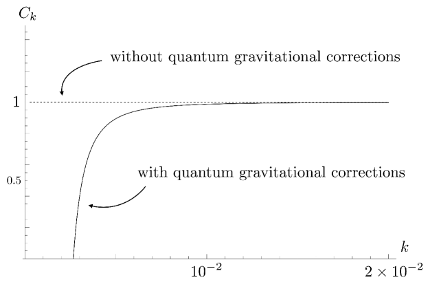
Figure 1: The function $C_{k}$ for $H=10^{14}\ {\rm GeV}$.

One therefore gets a concrete prediction from a conservative approach to quantum gravity: there must be a suppression of power at large scales. At present, there is no unambiguous observation of such an effect [6]. Therefore, one only gets an upper bound on the Hubble parameter $H$ [4],

$$H\lesssim 1.4\times 10^{-2}\,m_{\text{P}}\approx 4\times 10^{17}\,\text{GeV}.$$ (4)

This is, in fact, a weaker bound than the observational bound from the tensor-to-scalar ratio of the CMB fluctuations, which gives $H\lesssim 10^{-5}m_{\text{P}}\sim 10^{14}\,\text{GeV}$ (see, e.g., [8]); therefore, we have chosen the value $10^{14}\,\text{GeV}$ in Figure 1. Nevertheless, this investigation opens up a window to an energy range where quantum-gravitational effects can become large enough to be observable, in contrast to the situations hitherto studied.

One can also compare the above results with the predictions from other approaches to quantum gravity. Non-commutative geometry and effects from string theory also lead to a suppression of power at large scales, although of a different type [9]. This is not the case for loop quantum cosmology – there one finds an enhancement of power at large scales [10].

A comparison of these results could give us the unique opportunity to discriminate observationally between different approaches. To paraphrase Dyson’s words from above, the discovery of a small quantum-gravitational effect would clarify in a fundamental way our thinking about gravity, particles, and fields.

References

- [1] F. Dyson, in: Willis E. Lamb Jr.: A Festschrift on the Occasion of His 65th Birthday, ed. by D. ter Haar and M. O. Scully (North Holland, Amsterdam, 1978).
- [2] C. Kiefer, Quantum Gravity, third edition (Oxford University Press, Oxford, 2012).
- [3] C. Kiefer, Does time exist in quantum gravity? arXiv:0909.3767v1 [gr-qc].
- [4] C. Kiefer and M. Krämer, Phys. Rev. Lett. 108, 021301 (2012).
- [5] J. J. Halliwell and S. W. Hawking, Phys. Rev. D 31, 1777 (1985).
- [6] E. Komatsu et al., Astrophys. J. Suppl. Ser. 192, 18 (2011).
- [7] C. Kiefer and T. P. Singh, Phys. Rev. D 44, 1067 (1991).
- [8] D. Baumann et al., AIP Conf. Proc. 1141, 10 (2009).
- [9] S. Tsujikawa et al., Phys. Lett. B 574, 141 (2003); Y.S. Piao et al., Class. Quantum Grav. 21, 4455 (2004); G. Calcagni and S. Tsujikawa, Phys. Rev. D 70, 103514 (2004).
- [10] M. Bojowald, G. Calcagni, and S. Tsujikawa, Phys. Rev. Lett. 107, 211302 (2011).