Double Exchange Model in Triangular Lattice Studied by Truncated Polynomial Expansion Method

Abstract

The low temperature properties of double exchange model in triangular lattice are investigated via truncated polynomial expansion method (TPEM), which reduces the computational complexity and enables parallel computation. We found that for the half-filling case a stable 120^∘ spin configuration phase occurs owing to the frustration of triangular lattice and is further stabilized by antiferromagnetic (AF) superexchange interaction , while a transition between a stable ferromagnetic (FM) phase and a unique flux phase with small finite-size effect is induced by AF superexchange interaction for the quarter-filling case.

82B05,26C99,65F99,15A30

1 Introduction

Doped manganite has become one of the most important strongly correlated systems, since colossal magnetoresistance (CMR) effect was discovered in 1990s[1, 2]. CMR is referred to the resistivity of material change orders of magnitude under external magnetic field and it may have a potential application in computer technology or even spintronics. There are rich phase diagrams and many ordered phase[3], rising from delicate interaction between electron, spin and orbit degree of freedoms. Further it is found that the phase separation[4] (PS) may be crucial to CMR effect.

Double-exchange model, as a starting point to study manganite, describes the Hund interaction between itinerant electron and localized spin of Mn atoms and is expressed by

$$H_{DE}=-t\sum_{<ij>,\alpha}(C_{i,\alpha}^{{\dagger}}C_{j,\alpha}+h_{.}c_{.})-J_{H}\sum_{i,\alpha,\beta}C_{i,\alpha}^{{\dagger}}\sigma_{\alpha\beta}C_{i,\beta}\cdot S_{i},$$ (1)

where the nearest-neighbor hopping integral $t$ is adopted as the energy unit, $J_{H}$ is the Hund interaction strength, $C_{i,\alpha}^{{\dagger}}$ ($C_{i,\alpha}$) creates (annihilates) one electron at site $i$ with spin $\alpha$, $<ij>$ stands for the nearest neighbors of lattice site, and $\sigma_{\alpha\beta}$ is the Pauli matrix. The localized spin $S_{i}$ at site $i$ is assumed as $1$ here. In addition, antiferromagnetic (AF) superexchang is crucial to stabilize AF phase of some underdopped narrow-band manganite, and this interaction is expressed by $H_{AF}=J_{AF}\sum_{<ij>}S_{i}\cdot S_{j}$. So the total hamiltonian is $H=H_{DE}+H_{AF}$. In this model, localized spins is treated as a classic field $\phi$ and electron degree of freedom can be integrated for any given localized spin configuration. The partition function is expressed by $Z=\text{Tr}_{\text{c}}\text{Tr}_{\text{F}}(e^{-\beta[H(\phi)-\mu n_{e}]})=\text{Tr}_{\text{c}}e^{-S_{\text{eff}}(\phi)}$, and the effective action is $S_{\text{eff}}(\phi)=-\sum_{\nu}\ln(1+e^{-\beta(\epsilon_{\nu}-\mu)})+\beta E(\phi)$. Here $\epsilon_{\nu}$ is the $\nu$-th eigenvalue of one-electron sector’s Hamiltionian matrix $H(\phi)$, $E(\phi)$ is the interaction energy between spins, $\beta$ is the inverse temperature, $\mu$ is the chemical potential, and $n_{e}$ is the electron number operator, respectively. The fluctuation of localized spins is suitable for Monte Carlo (MC) simulation, and the partition sum is replaced by stochastic samplings with the Boltzmann weight $e^{-S_{\text{eff}}(\phi)}/Z$. With MC simulation, an intrinsic PS between high electron density and low electron density has been reproduced in doped maganites[5].

Despite the success of reproducing PS, the above method is suffered from finite-size effect, since the computational complexity of exact diagonalizing (DIAG) $H(\phi)$ scales as $O(N^{4})$, with $N$ being the system size. In order to overcome the above restriction, Furukawa and Motome [6, 7] proposed Chebyshev polynomials expansion method(PEM) and the computational complexity became $O(MN^{3})$ at a finite cutoff $M$. In 2004 they further reduced the computational complexity to $O(N)$ via truncated polynomial expansion method (TPEM)[8, 9]. The system size[10] is extended to $40\times 40$, compared with $10\times 10$ via DIAG[5]. Not only the computational complexity is greatly reduced, but also parallel computation is capable under PEM and TPEM, which would increase the computational speed very much. Finally, from the viewpoint of physical properties, one-body quantity such as energy and electron density, but also dynamical quantity or two-body quantity such as conductance are able to be investigated under PEM and TPEM, and there have been several examples of application to large scale system[10, 11, 12, 13].

Up to date, most studies focus on the double-exchange model in one- and two-dimensional square lattice. In this paper, we present our results on this model in two dimensional triangular lattice. One famous layered triangular lattice is the superconductor $Na_{0.35}CoO_{2}\cdot 1.35H_{2}O$ discovered in 2003 [14]. Though triangular lattice structure is not found in maganite yet, it is still meaningful to study the interplay between electron, spin and lattice for double exchange model in two dimensional triangular lattice. With the frustration, there is 120^∘ spin configuration in low temperature for the half-filling case, and this phase becomes more stable by AF superexchange interaction; but for the quarter-filling case, we found a stable long-range ferromagnetic (FM) ordered phase turns into a unique flux phase induced by AF superexchange interaction. This paper is arranged as follows: we briefly describe PEM and TPEM (more details please refer to Ref. [6, 7, 8, 9]) and give some benchmark in Sec 2, in Sec 3 show results in triangular lattice, and finally we summarize in Sec 4.

2 The method and benchmark

The core of Chebyshev polynomial expansion method (PEM) is that the mean value of physical quantity is expressed by the sum of the moment multiplied with physical quantity expansion coefficients, and it converges to exact value guaranteed by rapidly decaying expansion coefficients. It is important that the accuracy is controlled only by the cutoff $M$, the thresholds $\epsilon_{p}$ and $\epsilon_{tr}$, not by the system size and/or the chemical potential. It is further verified that the error does not accumulate with Monte Carlo sweep. It is advantageous that the application to large-scale system is capable, as the computational speed is greatly improved due to reduced computational complexity. In following, we will give a brief description of PEM and TPEM, and some benchmark.

2.1 Polynomial Expansion Method

The Chebyshev polynomials $T_{m}(x)$ are recursively defined by: $T_{0}(x)=1$, $T_{1}(x)=x$, and $T_{m}(x)=2xT_{m-1}(x)-T_{m-2}(x)$, with $-1\leq x\leq 1$. These polynomials are orthonormal in a form that

$$\int_{-1}^{1}\frac{dx}{\sqrt{1-x^{2}}}T_{m}(x)T_{m^{{}^{\prime}}}(x)=\alpha_{m}\delta_{mm^{{}^{\prime}}},$$

where $\alpha_{m}=\left\{\begin{array}[]{r@{\quad,\quad}l}1&m=0,\\ \frac{1}{2}&m\neq 0.\end{array}\right.$ The density of states (DOS) can be expressed as $D(\epsilon)=\frac{1}{2\pi\sqrt{1-\epsilon^{2}}}\sum_{m=0}^{\infty}\mu_{m}T_{m}(\epsilon)$, with the moment being $\mu_{m}=\int_{-1}^{1}T_{m}(\epsilon)D(\epsilon)d\epsilon$. Then the mean value of any physical operator $f$ can be expressed by

$$<f>=\int_{-1}^{1}d\epsilon D(\epsilon)f(\epsilon)=\sum_{m}\mu_{m}f_{m},$$ (2)

with expansion coefficients $f_{m}=\frac{1}{\alpha_{m}}\int_{-1}^{1}\frac{dx}{\sqrt{1-x^{2}}}f(x)T_{m}(x)$, which decay exponentially for $m\gg 1$ and ensure the accuracy at finite cutoff $M$[7]. Here $f(x)$ may be the effective action function $S(x)=-\ln[1+e^{\beta(x-\mu)}]$ or electron number function $n(x)=1/[1+e^{\beta(x-\mu)}]$, and $f_{m}$ is easily calculated.

The moment $\mu_{m}=\sum_{\nu=1}^{N_{\text{dim}}}T_{m}(\epsilon_{\nu})=Tr(T_{m}(H))$ can be evaluated under any set of orthonormal basis $e(k)$,

$$\mu_{m}=\sum_{k=1}^{N_{\text{dim}}}<e(k)|T_{m}(H)|e(k)>=\sum_{k=1}^{N_{\text{dim}}}\mu_{m}(k),$$ (3)

Here we define a vector $v(k,m)=T_{m}(H)|e(k)>$ and a partial moment $\mu_{m}(k)=<e(k)|v(k,m)>$. From the definition, it is easy to calculate the vector $v(k,m)$ recursively and the element $i$ in the vector $v(k,m)$ is expressed as

$$v_{i}(k,0)=e_{i}(k),$$

$$v_{i}(k,1)=\sum_{j}H_{ij}v_{j}(k,0),$$

$$v_{i}(k,m)=2\sum_{j}H_{ij}v_{j}(k,m-1)-v_{i}(k,m-2).$$ (4)

2.2 Truncation of Matrix-vector Product and Trace Operator

For a sparse hamiltonian matrix $H_{ij}$ with $O(N)$ nonzero elements, the multiplication can be confined to nonzero elements that scale as $O(M^{D})$ where $D$ is the system dimension. The computational complexity of $M$-th moment $\mu_{M}(k)$ is $O(M^{D+1})$ and further reduced to $O(M^{D/2+1})$ if elements less than the threshold $\epsilon_{p}$ are neglected. A subspace $N_{\epsilon_{p}}(k,m)$ is defined by $N_{\epsilon_{p}}(k,m)=\bigcup_{m^{{}^{\prime}}=0}^{m}\{i\},|v_{i}(k,m^{{}^{\prime}})|\geq\epsilon_{p}$. The total error of the Boltzmann weight is $O(M^{D+1}\epsilon_{p})$.

Based on the importance sampling method, during each MC sweep a new configuration is accepted as the ratio $r=\exp^{-\triangle S_{\text{eff}}}$ is larger than a random number uniformly distributed between 0 and 1. The update of the effective action $\triangle S_{\text{eff}}=\sum_{mk}[\mu_{m}^{\text{new}}(k)-\mu_{m}^{\text{old}}(k)]S_{m}$ is expressed by

$$\triangle S_{\text{eff}}=\sum_{m}S_{m}\sum_{k=1}^{N_{\text{dim}}}\triangle\mu_{m}(k),$$ (5)

and the update of the moment is

$$\triangle\mu_{m}(k)=<e(k)|v^{\text{new}}(k,m)>-<e(k)|v^{\text{old}}(k,m)>.$$ (6)

Due to local update of the classical field, only a few elements of the Hamiltonian matrix $H$ are modulated, there are only a limited amount of $v(k,m)$ to be updated, and a new threshold $\epsilon_{\text{tr}}$ can be taken to reduce the computational complexity. The total computational complexity of one MC sweep is $O(M^{D+1}N)$. As Eq. (3) is shown, each basis is inter-independent and the calculation of the moment $\mu_{m}$ can be parallelized.

2.3 Benchmark for double exchange model

Here we present some benchmark, such as the accuracy of the physical quantity, the number of nonzero elements, and the sweep time. One basic factor of the algorithm is the accuracy. As we mention above, the error can be controlled systematically by $M$, $\epsilon_{\text{p}}$ and $\epsilon_{\text{tr}}$, and the result is often reliable at finite $M$. In Fig. 1 we show the error of the effective action $S_{\text{eff}}$ and the electron occupation $n_{e}$ under a random spin configuration in two dimensional triangle lattice. As $M$ increases, the error is smaller and smaller, and the result eventually converges to the exact value. From Fig. 1(a-b), both the effective action and the electron density are very accurate for $20\leq M\leq 40$, though $M\sim 40$ is required at lower temperature due to slowly decaying $f_{m}$. Fortunately, the error does not depend on other physical parameters, such as the chemical potential $\mu$ (Fig. 1(c-d)) and the system size (Fig. 1(e-f)). Moreover, the error of the effective action does not accumulate during Monte Carlo update process (not shown here). These facts show that PEM combined with MC simulation is reliable to study large-scale system.

Figure 1: The error of $S_{eff}$ (a, c, e) and $n_{e}$ (b, d, f) vs the cutoff $M$ for a given spin configuration in triangular lattice. $J_{H}=8$ and $J_{AF}=0$. Other parameters are (a) and (b) $N=6\times 6$, $\mu=-8$; (c) and (d) $N=6\times 6$, $\beta=50$ ; and (e) and (f) $\beta=50$, $\mu=-8$.

The other important factor of the algorithm is the computation speed controlled by computational complexity. For TPEM, the complexity is usually associated with $N$, the system dimension $D$, $M$, $\epsilon_{\text{p}}$ and $\epsilon_{\text{tr}}$. In Fig. 2(a), we show how the number of elements in the subspace $N_{\epsilon_{\text{p}}}$ ($N_{e}$) change with $N$. While not surprisingly $N_{e}$ decreases with higher $\epsilon_{\text{p}}$, it is interesting that $N_{e}$ saturates no matter how large $N$ is. That is why the complexity is linear with $N$ for one MC sweep. In Fig. 2(b-c) the asymptotic behavior of $N_{e}$ changes from $O(M^{D})$ to $O(M^{D/2})$ once the truncation $\epsilon_{\text{p}}$ is taken.

Figure 2: $N_{e}$ elements in the subspace $N_{\epsilon_{p}}$ vs (a) the system size $N$ in one dimension, and vs (b, c) the cutoff $M$ in one and two dimension. $\beta=75$, $J_{H}=8$, $\mu=-8$, $J_{AF}=0$. (a) $M=16$, (b) $N=40$, and (c) $N=40\times 40$.

Now we compare the computational speed. Fig. 3 illustrates the CPU time cost by one MC sweep via DIAG and TPEM, respectively. In one dimension TPEM is prior as $N\geq 64$, and it is 1000 times faster than DIAG at $N\geq 512$. In two dimension, TPEM is advantageous as the system is larger than $14\times 14$. The sweep time is the same in square lattice and triangular lattice by DIAG , but it is shorter in square lattice than in triangular lattice by TPEM, as the hamiltonian is sparser owning to electron hopping between less nearest-neighbors in square lattice. Due to the dimensionality, the scaling behavior of time with respect to the system size is the same in triangular lattice as in square lattice. Once parallel computation is realized, TPEM will be more efficient.

Figure 3: Comparison of one MC sweep CPU time (sec) via TPEM and DIAG in (a) one and (b) two dimension. $M=30$, $\epsilon_{pr}=10^{-5}$ and $\epsilon_{tr}=10^{-3}$.

3 Double Exchange Model in Triangular Lattice

In triangular lattice with the lattice constant $a$, two basic lattice vectors are $\vec{a}_{1}=(1,0)a$ and $\vec{a}_{2}=(\frac{1}{2},\frac{\sqrt{3}}{2})a$. The reciprocal lattices are $\vec{b}_{1}=\frac{4\pi}{\sqrt{3}a}(\frac{\sqrt{3}}{2},-\frac{1}{2})$ and $\vec{b}_{2}=\frac{4\pi}{\sqrt{3}a}(0,1)$. For $L\times L$ triangular lattice, the momentum $\vec{q}=\frac{m}{L}\vec{b}_{1}+\frac{n}{L}\vec{b}_{2}$ is shortened as $(q_{1},q_{2})$, with $q_{1}=\frac{m}{L}$, $q_{2}=\frac{n}{L}$, and $m$, $n$ as integers from $0$ to $L$. Here we mainly focus on the spin structure factor $S(q)$ defined by

$$S(\vec{q})=\frac{1}{N}\sum_{i,j}<S_{i}\cdot S_{j}>e^{i\vec{q}\cdot\vec{r}_{ij}},$$ (7)

where $<S_{i}\cdot S_{j}>$ is the mean spin-spin correlation, $\vec{r}_{ij}$ is the displacement between site $i$ and $j$, and $N=L\times L$.

In order to understand the interplay between electron, spin and lattice, we study the spin-spin correlation for different filling case. First we will check the accuracy of the mean spin-spin correlation. The maximal monte carlo step is 10000, and the physical quantity is evaluated every 20 steps after first 2000 warmup steps. The parameters are $M=30$, $\epsilon_{p}=10^{-5}$ and $\epsilon_{tr}=10^{-3}$. Due to periodic boundary condition (PBC), we only show $<S_{1}\cdot S_{j}>$ with $1\leq j\leq N$ in Fig 4. For half-filling case (Fig. 4(a, d)) and low-filling case (Fig. 4(c, f)) regions, the accuracy are enough. But for quarter-filling case (Fig. 4(b)), the accuracy is not good, and higher $M$ is required. For the spin flux phase, $M=30$ is enough for the accuracy as Fig. 4(e) shows, and the accuracy was verified in $6\times 6$ to $12\times 12$ triangular lattice. Therefore it is not necessary to use large $M$ as the basic physical phenomenon still remains.

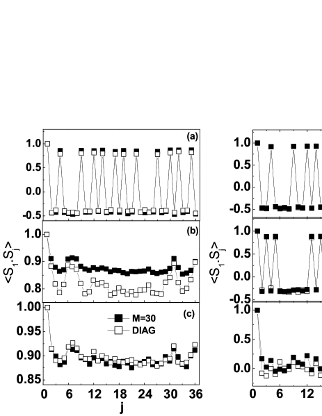
Figure 4: The spin-spin correlation $<S_{1}\cdot S_{j}>$ of $6\times 6$ triangular lattice. $\beta=75$ and $J_{H}=8$. $\epsilon_{p}=10^{-5}$ and $\epsilon_{tr}=10^{-3}$. (a) $J_{AF}=0$, $\mu=-6$ and $<n>=0.9272$, (b) $J_{AF}=0$, $\mu=-8$ and $<n>=0.4512$, (c) $J_{AF}=0$, $\mu=-10$ and $<n>=0.1944$, (d) $J_{AF}=0.1$, $\mu=-6$ and $<n>=0.9146$, (e) $J_{AF}=0.1$, $\mu=-8$ and $<n>=0.5$, (f) $J_{AF}=0.1$, $\mu=-10$ and $<n>=0.2101$.

3.1 Half-filling case

For half-filling case one lattice has one electron and electron hops between adjacent lattices will reduce the total energy. According to Pauli exclusion rule two electrons on one lattice site should have opposite spins, hence the nearest-neighbor localized spins tend to be antiparallel, but there exists frustration effect induced by triangular lattice. Therefore 120^∘ spin configuration occurs, where three localized spins of each triangle are coplaner with angle between any two being 120^∘. Using the method in Ref. [16], the coplane is verified by the fact that $(S_{i}\times S_{j})\cdot S_{k}$ statistically equals to zero, where site $i$, $j$ and $k$ are located in one triangle; and the angle between any two being 120^∘ is verified by the spin-spin correlation of adjacent sites being $-0.48$, very close to the limit $-0.5$. Regarding to $S(\vec{q})$, two peaks are located at $(\frac{1}{3},\frac{1}{3})$ and $(\frac{2}{3},\frac{2}{3})$, respectively, and $S(\vec{q})/N=0.408$ (Fig. 5(a)). This phase is stabilized by AF superexchange interaction with $S(\vec{q})/N=0.464$(Fig. 5(d)).

3.2 Low- and Mediate-filling case

For low- and mediate-filling case, there is less than one electron on each lattice site and adjacent spins tend to be parallel. Hence the system is in FM phase and the peak $S(\vec{0,0})/N=0.821$ is close to the maximum value 1 (Fig. 5(c)). But in the presence of superexchange interaction, the system is paramagnetic (Fig. 5(f)) because of the competition between electron-mediated FM correlation and AF superexchange interaction. The spin structure factor is almost flat at all vector $\vec{q}$ and has no peak at all. But for near zero filling case, 120^∘ spin configuration will be induced by AF interaction with the interplay between spins and lattice.

3.3 Quarter-filling case

For quarter-filling case in one- and two-dimensional square lattice with PBC, the FM phase is not stable, that is positive spin-spin correlation at short distance and negative at long distance. This phenomenon has been observed long before (Ref. [5] and the Reference inside). Open boundary condition (OBC) or other kind of boundary condition is chosen to stabilize FM phase[5]. In two-dimensional triangular lattice with PBC, the effect of lattice on FM phase is significant. Each site has 6 nearest-neighbors, and their spins tend to be parallel. It is found that electron-mediated FM phase is stablized even at long distance and $S(0,0)/N=0.899$(Fig. 5(b)). So the FM phase is strengthened by triangular lattice, compared with square lattice.

Now we consider the effect on AF superexchange interaction on spin-spin correlation. A spin-flux phase[10, 16] occurs in the square lattice, where four localized spins within each square lie (anti)clockwise at the same plane. In the triangular lattice, as $J_{AF}$ increases from 0 to $0.4$ (in fact $J_{AF}$ does not exceed 0.1 in material), the system is in FM phase at first and then turns into a specific flux phase and eventually evolves into 120^∘ spin configuration phase. For the specific flux phase corresponding to the mediate AF superexchange interaction, $(S_{i}\times S_{j})\cdot S_{k}$ with the sites $i$, $j$ and $k$ belonging to one triangle statistically equals to $0.7$, and the spin-spin correlation of adjacent sites is $-0.3$. So this phase is different from both FM phase and 120^∘ configuration phase. The peak $S(\vec{q})$ is located at vectors $(\frac{1}{2},0)$, $(0,\frac{1}{2})$ and $(\frac{1}{2},\frac{1}{2})$, respectively, and $S(\vec{q})/N\sim 0.29$ very close to its maximum value 1/3 (Fig. 5(e)). We further extend the system size from $6\times 6$ to $12\times 12$, and find that the peaks position does not change and the normalized peak value $S(\vec{q})/N$ converges to 0.285 (Fig. 6). So finite-size effect is small and this flux phase is very stable.

We systematically investigate the behavior of the spin-spin correlation and spin structure factor at high temperature. The peak value of spin structure factor decreases with the temperature, and eventually at beta=10 the system is paramagnetic as $J_{AF}$ ranges from 0 to 0.1. So there is no phase transition at high temperature and the system is still subjected to the dimensionality of system.

Figure 5: The spin structure factor $S(q_{1},q_{2})$ of $6\times 6$ triangular lattice. $\beta=75$, and $J_{H}=8$. (a) $J_{AF}=0$, $\mu=-6$ and $<n>=0.9272$, (b) $J_{AF}=0$, $\mu=-8$ and $<n>=0.4512$, (c) $J_{AF}=0$, $\mu=-10$ and $<n>=0.1944$, (d) $J_{AF}=0.1$, $\mu=-6$ and $<n>=0.9146$, (e) $J_{AF}=0.1$, $\mu=-8$ and $<n>=0.5$, and (f) $J_{AF}=0.1$, $\mu=-10$ and $<n>=0.2101$.

Figure 6: The peak $S(\vec{q})$ vs the size $L$ in two dimensional triangular lattices. $\beta=75$, $J_{H}=8$, $J_{AF}=0.1$, $\mu=-8$ and $<n>=0.5$.

4 Conclusion

Double exchange model with antiferromagnetic spin-spin superexchange interaction has been studied for two dimensional triangular lattice with the truncated polynomial expansion method. For the half-filling case we obtained 120^∘ spin configuration at low temperature, and it is further stabilized by superexchange ineraction. For the quarter-filling case, we found that the FM phase is quite stable, and superexchange interaction results in a unique spin-flux configuration with very small finite-size effect.

References

- [1] R. von Helmot, J. Wecker, B. Holzapfel, L. Schultz and K. Samwer, Phys. Rev. Lett., 71 (1993), 2331.
- [2] S. Jin, T. H. Tiefel, M. McCormakc, R. A. Fastnacht, R. Ramesh, and L. H. Chen, Science, 264 (1994), 413.
- [3] A. Urushibara, Y. Moritomo, T. Arima, A. Asamitsu, G. Kido, and Y. Tokura , Phys. Rev. B, 51 (1995), 14103.
- [4] Y.-D. Chuang, A. D. Gromko, D. S. Dessau, T. Kimura, and Y. Tokura, Science, 292 (2001), 1509.
- [5] S. Yunoki, J. Hu, A. L. Malvezzi, A. Moreo, N. Furukawa, and E. Dagotto, Phys. Rev. Lett., 80 (1998), 845.
- [6] Y. Motome, N. Furukawa, J. Phys. Soc. Jpn., 68 (1998),3853.
- [7] N. Furukawa, Y. Motome, Comput. Phys. Comm., 142 (2001), 410.
- [8] N. Furukawa, Y. Motome, J. Phys. Soc. Jpn., 73 (2004), 1482.
- [9] G. Alvarez, C. Sen, N. Furukawa, Y. Motome, and E. Dagotto, Comput. Phys. Commu., 168 (2005), 32.
- [10] C. Sen, G. Alvarez, Y. Motome, N. Furukawa, I. A. Sergienko, T. C. Schulthess, A. Moreo, and E. Dagotto, Phys. Rev. B, 73 (2006), 224430.
- [11] G. Alvarez, T. C. Schulthess, Phys. Rev. B, 73 (2006), 035117.
- [12] G. Alvarez, H. Aliaga, C. Sen, and E. Dagotto, Phys. Rev. B, 73 (2006) , 224426.
- [13] C. Sen, G. Alvarez, H. Aliaga, and E. Dagotto, Phys. Rev. B, 73 (2006), 224441.
- [14] T. Takada, H. Sakurai, E. Takayama-Muromachi, F. Izumi, R. A. Dilanian and and T. Sasaki, Nature, 422 (2003), 53.
- [15] J. L. Alonso, L. A. Fernández, F. Guinea, V. Laliena, and V. Martín-Mayo, Nucl. Phys. B, 596 (2001), 587.
- [16] D. F. Agterberg and S. Yunoki, Phys. Rev. B, 62 (2000), 13816.