S-duality as a $\beta$-deformed Fourier transform

ABSTRACT

An attempt is made to formulate Gaiotto’s S-duality relations in an explicit quantitative form. Formally the problem is that of evaluation of the Racah coefficients for the Virasoro algebra, and we approach it with the help of the matrix model representation of the AGT-related conformal blocks and Nekrasov functions. In the Seiberg-Witten limit, this S-duality reduces to the Legendre transformation. In the simplest case, its lifting to the level of Nekrasov functions is just the Fourier transform, while corrections are related to the beta-deformation. We calculate them with the help of the matrix model approach and observe that they vanish for $\beta=1$. Explicit evaluation of the same corrections from the $U_{q}(sl(2))$ infinite-dimensional representation formulas due to B.Ponsot and J.Teshner remains an open problem.

1 Introduction

Conformal blocks (CB) naturally arise in consideration of multi-point correlation functions in CFT [1]. They provide the holomorphic factorization of correlation functions. Note that anomaly free symmetries of the correlation functions are lost after the holomorphic factorization. Instead, under the modular transformation the CB are linearly transformed with the help of matrix of the Racah-Wiegner coefficients, which relates different ways to rearrange the brackets in associative tensor product [2]. A straightforward computation of these fusion relations from basic principles of CFT is still available only for degenerate representations. Study of this problem in a general context might reveal some hidden integrable structures in related theories.

Another possible approach [3] is based on a similar construction for alternative ”conformal blocks” for ${\cal U}_{q}(sl_{2})$. This problem is technically simpler, and surprisingly the additional deformation parameter $q$ turns to be related to the central charge $c$ of the Virasoro algebra.

In fact, the Racah-Wiegner coefficients, being a basic notion of representation theory, are important for quite different subjects. The recently discovered AGT conjecture [4, 5] seems to be especially interesting in this context, since it relates modular properties of the conformal block with a weak-strong coupling S-duality in ${\cal N}=2$ SUSY gauge (SYM) theories. The problem is that the $S$-duality [6] is rather well-understood for the low-energy effective action in the Seiberg-Witten (SW) theory [7, 8, 9, 10], while the conformal block is AGT-related with the Nekrasov functions [11] (which describe the $\Omega$-background deformation of the original SYM theory [12]) with two non-vanishing parameters $\epsilon_{1},\epsilon_{2}\neq 0$, where the $S$-duality transformations remain unknown. Therefore, the equivalence between the $S$- and modular dualities, which has to be an essential part of the AGT relation, still lacks any kind of quantitative description. The purpose of this paper is to initiate consideration of this non-trivial problem.

We begin with the simple and nice functional interpretation of the $S$-duality in the limit of $\epsilon_{1}=\epsilon_{2}=0$, i.e. with the SW theory. In this case, the SW prepotential $F(a)$ depending on the scalar vacuum expectation value (v.e.v.) of the SYM theory, and its S-dual $F^{*}(b)$ are related by a simple Legendre transform

$$F^{*}(b)=\sup\limits_{a}(F(a)-ab),$$ (1)

what can be considered as a saddle point approximation to the Fourier integral transform

$$\exp\left\{\frac{2\pi i}{\epsilon_{1}\epsilon_{2}}F^{*}(b)\right\}=\int da\exp\left\{-\frac{2\pi iab}{\epsilon_{1}\epsilon_{2}}\right\}\exp\left\{\frac{2\pi i}{\epsilon_{1}\epsilon_{2}}F(a)\right\},\quad\epsilon_{1,2}\rightarrow 0$$ (2)

The question is how the Fourier transform is deformed when $\epsilon_{1},\epsilon_{2}\neq 0$. Technically, the simplest way to calculate corrections is to use the matrix model description [13, 14] of the conformal blocks and the Nekrasov functions. Here the Seiberg-Witten limit and the Fourier transform are just properties of the spherical limit (the leading order in the genus expansion), and the higher order corrections can be restored by well-prescribed procedures like the topological recursion [15]. Surprisingly, the Fourier transform does not acquire corrections in the case of $\beta=1$, at least, in the lowest orders, though there are non-trivial corrections in the case of $\beta\neq 1$. It would be nice to develop some technique that would allow one to reproduce these corrections in other approaches.

Another interesting research direction is impled by the fact of appearance of the Racah coefficients in the modular transformations and in description of the HOMFLY polynomials [16]. This is a road to the most interesting versions of the $3d$ AGT relations [17], but it is beyond the scope of the present paper.

The paper is organized as follows. We briefly describe in sect.2 what are the Racah-Wiegner coefficients for the Virasoro algebra and their simulation due to [3]. In sect.3 we review the AGT relation in the form we need in our further consideration. Formulas for the Racah-Wiegner coefficients in particular cases, when they are given by the Fourier transform are discussed in sect.4. At last, in sect.5 we develop the general technique based on matrix model representation and, as an illustration, calculate a few first corrections to the Fourier transform. Sect.6 contains comments on $S$-duality transformations in the limit of $\epsilon_{2}\to 0$.

2 Racah-Wiegner coefficients for the Virasoro algebra [18]

2.1 Some definitions

As is well-known, $2d$ conformal field theories can be interpreted in terms of representation theory of the Virasoro algebra,

$$\left[L_{n},L_{m}\right]=(n-m)L_{n+m}+\frac{c}{12}n(n^{2}-1)\delta_{n+m}$$ (3)

with a non-trivial co-multiplication rule [18]

$${\bf\Delta}(L_{n})=I\otimes L_{n}+\sum_{k=-1}^{\infty}x^{n-k}\left({n+1}\atop{k+1}\right)L_{k}\otimes I$$ (4)

which preserves the central charge of the algebra (the central charge of the naive co-multiplication $\tilde{\bf\Delta}(L_{n})=I\otimes L_{n}+L_{n}\otimes I$ is twice as large as that of $L_{n}$). We denote the co-multiplication with the bold letter in order to distinguish it from the dimensions of conformal fields. The primary fields correspond to the highest weight vectors $L_{Y}V_{\Delta}=0$, $L_{0}V_{\Delta}=\Delta V_{\Delta}$, which generate representations (Verma modules) $R_{\Delta}=\Big{\{}L_{-Y}V_{\Delta}\Big{\}}$. The chiral part of the associative operator product expansion

$$L_{-Y_{1}}V_{\Delta_{1}}(0)\otimes L_{-Y_{2}}V_{\Delta_{2}}(x)=\sum\limits_{\Delta,Y}C^{\Delta,Y}_{\Delta_{1},Y_{1}|\Delta_{2},Y_{2}}L_{-Y}V_{\Delta}(0)\,x^{\Delta+|Y|-\Delta_{1}-|Y_{1}|-\Delta_{2}-|Y_{2}|}$$ (5)

has to be compatible with (4), which severely restricts (almost fixes) the coefficients $C^{\Delta,Y}_{\Delta_{1},Y_{1}|\Delta_{2},Y_{2}}$.

However, there is more than just the associative algebra structure. The four-point conformal block is given by the scalar product of a triple product of representations with fixed representation in the intermediate channel and the representation associated with the infinity point (further we associate it with the fourth point of the CB). More exactly, one considers the product of two intertwining operators, $\Phi_{12}^{3}:R_{1}\otimes R_{2}\longrightarrow R_{3}$ which can be combined in two different ways: $\Phi_{\Delta_{1},\Delta_{2}}^{\Delta}\Phi_{\Delta,\Delta_{3}}^{\Delta_{4}}$ and $\Phi_{\Delta_{1},\Delta}^{\Delta_{4}}\Phi_{\Delta_{2},\Delta_{3}}^{\Delta}$, where the intermediate representation $R_{\Delta}$ labels different representations emerging in the tensor product of two representations. As usual in representation theory, one demands the co-multiplication to be associative, which means that the two different products of intertwining operators give just two different bases of conformal blocks related by an orthogonal $x$-independent matrix $M_{\Delta\Delta^{\prime}}$ which is called the Racah-Wiegner matrix, i.e. by a linear map

$$\Phi_{\Delta_{1},\Delta_{2}}^{\Delta}\Phi_{\Delta,\Delta_{3}}^{\Delta_{4}}=\sum\limits_{\Delta^{\prime}}M_{\Delta\Delta^{\prime}}\Phi_{\Delta_{1},\Delta^{\prime}}^{\Delta_{4}}\Phi_{\Delta_{2},\Delta_{3}}^{\Delta^{\prime}}$$ (6)

Instead of considering these products of intertwining operators, one can calculate their value on the highest weight vectors. Since the dual of $R_{\Delta_{4}}$ enters the answer, it can be written using the scalar product. This product is called the conformal block and, thus, there are two essentially different conformal blocks. They can be presented pictorially as

(13)

In terms of the conformal blocks relation (6) can be rewritten as

$$\boxed{B_{\Delta}(x)=\sum\limits_{\Delta^{\prime}}M_{\Delta\Delta^{\prime}}B_{\Delta^{\prime}}(1-x)}$$ (14)

Our goal is to study this map within the context of AGT. On one side, $M_{\Delta\Delta^{\prime}}$ describes modular transformations of the conformal block. On another side, it is a deformation of the Legendre transform (1) to $\epsilon_{1},\epsilon_{2}\neq 0$.

2.2 Various modular transformations

It is worth noticing that relation (14) does not exhaust all possible relations between different types of conformal blocks. Indeed, one could change the order of vertex operators inside the brackets and rearrange the brackets in different way in the final scalar product. In fact, one can construct all possible different relation by two independent transformations

$$\hat{S}:\ \ \ \ \ x\to 1-x,\ \ \ \ \hat{T}:\ \ \ \ \ x\to{x\over x-1}$$ (15)

The first transformation connects the following two conformal blocks

$$\begin{picture}(30.0,14.0)\put(0.0,0.0){\line(1,0){30.0}} \put(10.0,0.0){\line(0,1){10.0}} \put(20.0,0.0){\line(0,1){10.0}} \put(1.0,2.0){\makebox(0.0,0.0)[cc]{$0,\Delta_{1}$}} \put(6.0,9.0){\makebox(0.0,0.0)[cc]{$x,\Delta_{2}$}} \put(15.0,2.0){\makebox(0.0,0.0)[cc]{$\Delta$}} \put(16.0,9.0){\makebox(0.0,0.0)[cc]{$1,\Delta_{3}$}} \put(30.0,2.0){\makebox(0.0,0.0)[cc]{$\infty,\Delta_{4}$}} \end{picture}\qquad\mathop{\longrightarrow}^{\hat{S}}\qquad\begin{picture}(30.0,14.0)\put(0.0,0.0){\line(1,0){30.0}} \put(10.0,0.0){\line(0,1){10.0}} \put(20.0,0.0){\line(0,1){10.0}} \put(1.0,2.0){\makebox(0.0,0.0)[cc]{$1,\Delta_{3}$}} \put(6.0,9.0){\makebox(0.0,0.0)[cc]{$x,\Delta_{2}$}} \put(15.0,2.0){\makebox(0.0,0.0)[cc]{$\Delta^{\prime}$}} \put(16.0,9.0){\makebox(0.0,0.0)[cc]{$0,\Delta_{1}$}} \put(30.0,2.0){\makebox(0.0,0.0)[cc]{$\infty,\Delta_{4}$}} \end{picture}$$ (16)

This $S$-duality transformation looks especially simple in terms of the ”the effective coupling constant” ${\cal T}$ (see s.3.1 below for the explanation of the terminology) in the SW limit:

$$\hat{S}:\quad{\cal T}\rightarrow-\frac{1}{\cal T}$$ (17)

The second generator, $\hat{T}$ which describes the second modular transformation (the two being enough to give rise to the whole modular group), in this case looks like

$$\hat{T}:\quad{\cal T}\rightarrow{\cal T}+1$$ (18)

This transformation connects the following conformal blocks

$$\begin{picture}(30.0,14.0)\put(0.0,0.0){\line(1,0){30.0}} \put(10.0,0.0){\line(0,1){10.0}} \put(20.0,0.0){\line(0,1){10.0}} \put(1.0,2.0){\makebox(0.0,0.0)[cc]{$0,\Delta_{1}$}} \put(6.0,9.0){\makebox(0.0,0.0)[cc]{$x,\Delta_{2}$}} \put(15.0,2.0){\makebox(0.0,0.0)[cc]{$\Delta$}} \put(16.0,9.0){\makebox(0.0,0.0)[cc]{$1,\Delta_{3}$}} \put(30.0,2.0){\makebox(0.0,0.0)[cc]{$\infty,\Delta_{4}$}} \end{picture}\qquad\mathop{\longrightarrow}^{\hat{T}}\qquad\begin{picture}(30.0,14.0)\put(0.0,0.0){\line(1,0){30.0}} \put(10.0,0.0){\line(0,1){10.0}} \put(20.0,0.0){\line(0,1){10.0}} \put(1.0,2.0){\makebox(0.0,0.0)[cc]{$0,\Delta_{1}$}} \put(6.0,9.0){\makebox(0.0,0.0)[cc]{$x,\Delta_{2}$}} \put(15.0,2.0){\makebox(0.0,0.0)[cc]{$\Delta^{\prime}$}} \put(16.0,9.0){\makebox(0.0,0.0)[cc]{$\infty,\Delta_{4}$}} \put(30.0,2.0){\makebox(0.0,0.0)[cc]{$1,\Delta_{3}$}} \end{picture}$$ (19)

One can also use ”the bare coupling constant” $\tau_{0}$: $x=e^{2\pi i\tau_{0}}$ (see s.3.1), though in these terms the same transformations look quite ugly:

$$\hat{S}:\ \ \ \ \ e^{2\pi i\tau_{0}}\to 1-e^{2\pi i\tau_{0}},\ \ \ \ \hat{T}:\ \ \ \ \ e^{2\pi i\tau_{0}}\to{e^{2\pi i\tau_{0}}\over e^{2\pi i\tau_{0}}-1}$$ (20)

In the generic $\Omega$-background the conformal block transforms non-trivially only w.r.t. the first transformation, $\hat{S}$, while the $\hat{T}$-transformation just gives rise to a trivial factor:

$$B_{\Delta}\Big{(}\Delta_{1},\Delta_{2},\Delta_{3},\Delta_{4}|x\Big{)}=(-1)^{\Delta}(1-x)^{2\Delta_{2}}B_{\Delta}\Big{(}\Delta_{1},\Delta_{2},\Delta_{4},\Delta_{3}|x\Big{)}$$ (21)

This is because $\hat{T}$ interchanges the points $1$ and $\infty$ and does not affect the point $x$. At the same time, (14) is absolutely non-trivial transformation, so we mostly concentrate on it.

We shall also consider modular transformations of the one-point conformal block on a torus which depends on the modular parameter of the torus $\tau_{0}$. These modular transformations are generated by two independent transformations

$$\hat{S}:\ \ \ \ \ \tau_{0}\to-{1\over\tau_{0}},\ \ \ \ \hat{T}:\ \ \ \ \ \tau_{0}\to\tau_{0}+1$$ (22)

In this case also only the $\hat{S}$-transformation is non-trivial, while the $\hat{T}$-transformation just gives rise to a phase factor:

$$B_{\Delta}\Big{(}\Delta_{ext}|\tau_{0}+1\Big{)}=\exp\Big{\{}2\pi i\Big{(}\Delta-{c\over 24}\Big{)}\Big{\}}B_{\Delta}\Big{(}\Delta_{ext}|\tau_{0}\Big{)}$$ (23)

We return to discussion of the whole modular ($S$-duality) group in s.6.

2.3 Racah-Wiegner coefficients for Virasoro from ${\cal U}_{q}(sl_{2})$-representations

The problem of constructing the Racah-Wiegner matrix for the Virasoro algebra was solved in the case of degenerate representations [18], though in generic situation it is quite involved. Instead, in [3] B.Ponsot and J.Teschner studied the Racah-Wiegner matrix for specific infinite-dimensional representations of the algebra $U_{q}(sl_{2})$ and suggested that it is equal to that for the Virasoro case.

In fact, the modular transformation was explicitly described in [3] in two cases, AGT-related to $SU(2)$ SYM theory with $N_{f}=2N_{c}=4$ matter hypermultiplets or with one adjoint matter multiplet. The first case is the spherical four-point conformal block [3]:

$$B_{p}\left(\left.\begin{array}[]{cc}p_{1}&p_{2}\\ p_{3}&p_{4}\end{array}\right|x\right)=\int d\mu(p^{\prime})M_{pp^{\prime}}\left(\begin{array}[]{cc}p_{1}&p_{2}\\ p_{3}&p_{4}\end{array}\right)B_{p^{\prime}}\left(\left.\begin{array}[]{cc}p_{2}&p_{3}\\ p_{4}&p_{1}\end{array}\right|1-x\right)$$ (30)

where

$$\Delta(p)=\frac{\epsilon^{2}/4+p^{2}}{\epsilon_{1}\epsilon_{2}},\quad d\mu(p)=4\sinh\left(2\pi\frac{p}{\epsilon_{1}}\right)\sinh\left(2\pi\frac{p}{\epsilon_{2}}\right)dp,\ \ \ \ \ \ \ \epsilon=\epsilon_{1}+\epsilon_{2}$$ (31)

and

$$M_{pp^{\prime}}\left(\begin{array}[]{cc}p_{1}&p_{2}\\ p_{3}&p_{4}\end{array}\right)=\frac{s(u_{1})s(w_{1})}{s(u_{2})s(w_{2})}\int\limits_{\mathbb{R}}dt\prod\limits_{i=1}^{4}\frac{s(t-r_{i})}{s(t-q_{i})}$$ (34)

$$\begin{array}[]{cccc}r_{1}=p_{2}-p_{1}&q_{1}=\epsilon/2-p_{4}+p_{2}-p^{\prime}&u_{1}=p+p_{2}-p_{1}\\ r_{2}=p_{2}+p_{1}&q_{2}=\epsilon/2-p_{4}+p_{2}+p^{\prime}&u_{2}=p+p_{3}+p_{4}\\ r_{3}=-p_{4}-p_{3}&q_{3}=\epsilon/2+p&w_{1}=p^{\prime}+p_{1}+p_{4}\\ r_{4}=-p_{4}+p_{3}&q_{4}=\epsilon/2-p&w_{2}=p^{\prime}+p_{2}-p_{3}\\ \end{array}$$ (39)

while the second case is the one-point toric conformal block

$$B_{p}(p_{0}|{\cal T})=\int d\mu(p^{\prime})M_{pp^{\prime}}(p_{0})B_{p^{\prime}}(p_{0}|-1/{\cal T})$$ (40)

$$M_{pp^{\prime}}(p_{0})=\frac{2^{\frac{3}{2}}}{s(p_{0})}\int\limits_{\mathbb{R}}dt\frac{s\left(p^{\prime}+\frac{1}{2}(p_{0}+\epsilon)+t\right)s\left(p^{\prime}+\frac{1}{2}(p_{0}+\epsilon)-t\right)}{s\left(p^{\prime}-\frac{1}{2}(p_{0}+\epsilon)+t\right)s\left(p^{\prime}-\frac{1}{2}(p_{0}+\epsilon)-t\right)}e^{4\pi ipt}$$ (41)

where we used ”the quantum dilogarithm” [19], the ratio of two digamma-functions [20],

$$\log s(z|\epsilon_{1},\epsilon_{2})=\frac{1}{i}\int\limits_{0}^{\infty}\frac{dt}{t}\left(\frac{\sin 2xt}{2\sinh\epsilon_{1}t\sinh\epsilon_{2}t}-\frac{x}{\epsilon_{1}\epsilon_{2}t}\right)=$$

$$=\prod_{m,n\geq 0}\frac{\left(m+\frac{1}{2}\right)\epsilon_{1}+\left(n+\frac{1}{2}\right)\epsilon_{2}-iz}{\left(m+\frac{1}{2}\right)\epsilon_{1}+\left(n+\frac{1}{2}\right)\epsilon_{2}+iz}=\frac{\Gamma_{2}(\epsilon/2+iz|\epsilon_{1},\epsilon_{2})}{\Gamma_{2}(\epsilon/2-iz|\epsilon_{1},\epsilon_{2})}$$ (42)

which possesses a number of periodicity properties

$$s\left(z-\frac{i\epsilon_{2}}{2}\Big{|}\epsilon_{1},\epsilon_{2}\right)=2\cosh\left(\frac{\pi z}{\epsilon_{1}}\right)s\left(z+\frac{i\epsilon_{2}}{2}\Big{|}\epsilon_{1},\epsilon_{2}\right)$$ (43)

$$s\left(z-\frac{i\epsilon_{1}}{2}\Big{|}\epsilon_{1},\epsilon_{2}\right)=2\cosh\left(\frac{\pi z}{\epsilon_{2}}\right)s\left(z+\frac{i\epsilon_{1}}{2}\Big{|}\epsilon_{1},\epsilon_{2}\right)$$ (44)

$$s\left(z-\frac{i\epsilon}{2}\Big{|}\epsilon_{1},\epsilon_{2}\right)=4\sinh\left(\frac{\pi z}{\epsilon_{1}}\right)\sinh\left(\frac{\pi z}{\epsilon_{2}}\right)s\left(z+\frac{i\epsilon}{2}\Big{|}\epsilon_{1},\epsilon_{2}\right)$$ (45)

Formulas (30), (40) and (41) should be considered as contour integrals around poles and zeroes of the quantum dilogarithms and they are quite difficult to use. They can be simplified in some particular cases.

3 AGT representation for conformal block

3.1 Nekrasov partition function

The complex coupling constant in the Yang-Mills theory is defined in terms of the standard coupling constant $g$ and the $\theta$-angle as

$${\cal T}=\frac{4\pi i}{g^{2}}+\frac{\theta}{2\pi}$$ (46)

The internal symmetry transformation of the theory ${\cal T}\mapsto{\cal T}+1$ and the duality map (S-duality) defined by N.Seiberg and E.Witten [7], form the modular group $SL(2,\mathbb{Z})$. It is important to distinguish between the bare coupling constant $\tau_{0}$ arising in the fundamental SYM theory and the effective one, ${\cal T}$ arising in the low-energy effective action of the general form

$$S_{eff}=\frac{1}{4\pi}\int d^{4}x\,\Im\hbox{m}\left[\int d^{2}\theta\,\frac{\partial\mathcal{F}(A)}{\partial A}\bar{A}+\frac{1}{2}\int d^{4}\theta\,\frac{\partial^{2}\mathcal{F}(A)}{\partial A^{2}}W_{\alpha}W^{\alpha}\right]$$ (47)

as ${\cal T}(a)=\partial^{2}\mathcal{F}(a)/\partial a^{2}$, where the modulus $a$ is essentially the scalar field v.e.v. We are interested in action of S-duality on both ${\cal T}$ and $\tau_{0}$. The SW prepotential can be simply related [11] to the LMNS integral [21]

$$\mathcal{F}=\lim\limits_{\epsilon_{1,2}\rightarrow 0}\frac{\epsilon_{1}\epsilon_{2}}{2\pi i}\log\mathcal{Z}_{\rm LMNS}$$

The LMNS integral is defined for the ${\cal N}=2$ SYM theory on the so called $\Omega$-background parameterized by two parameters $\epsilon_{1}$ and $\epsilon_{2}$. The simplest is the theory with the gauge group $SU(2)$ and four fundamental matter hypermultiplets with masses $\mu_{i}$ (the $\beta$-function in this theory is vanishing). In this case, the LMNS integral is represented [11] by a power series in exponential of the bare coupling constant $\tau_{0}$ parameterized by pairs of the Young diagrams $Y_{1}$, $Y_{2}$

$$Z_{\rm Nek}=\sum\limits_{Y_{1},Y_{2}}N_{\epsilon_{1,2}}(Y_{1},Y_{2},\mu_{1},\mu_{2},\mu_{3},\mu_{4},a)e^{2\pi i\tau_{0}(|Y_{1}|+|Y_{2}|)}$$ (48)

The coefficients $N_{\epsilon_{1,2}}(Y_{1},Y_{2},\mu_{1},\mu_{2},\mu_{3},\mu_{4},a)$ (the Nekrasov functions) are rational functions in $\epsilon$’s, the scalar v.e.v. $a$, and the matter hypermultiplet masses $\mu_{i}$’s.

This series is known to coincide [4, 5, 22] with the four-point conformal block up to a so called $U(1)$-factor under the following identification of the CFT and SYM data:

$$\Delta(\alpha)=\frac{\alpha(\epsilon_{1}+\epsilon_{2}-\alpha)}{\epsilon_{1}\epsilon_{2}},c=1+6\frac{(\epsilon_{1}+\epsilon_{2})^{2}}{\epsilon_{1}\epsilon_{2}}$$ (49)

$$\mu_{1}=-\epsilon/2+\alpha_{1}+\alpha_{2},\quad\mu_{2}=\epsilon/2+\alpha_{2}-\alpha_{1},\quad\mu_{3}=-\epsilon/2+\alpha_{3}+\alpha_{4},\quad\mu_{4}=\epsilon/2+\alpha_{3}-\alpha_{4}$$ (50)

$$a=\alpha-\epsilon/2,\quad x=e^{2\pi i\tau_{0}}$$ (51)

where $\alpha_{i}$ corresponds to the four external dimensions and $\alpha$ to the intermediate dimension in (13).

It is remarkable that these Nekrasov functions do not possess any specific symmetry, though the Seiberg-Witten theory does [7, 8]. Indeed, the Seiberg-Witten theory is symmetric under the transformations

$$\hat{T}:\quad{\cal T}\rightarrow{\cal T}+1$$ (52)

$$\hat{S}:\quad{\cal T}\rightarrow-\frac{1}{{\cal T}}$$

This symmetry reflects the freedom in choosing the $A$- and $B$-cycles on the spectral curve. As we shall see, these symmetries can be lifted to the level of the $\epsilon$-deformed prepotential or the Nekrasov functions. The idea of this identification was presented in [23]. It is also supported by the fact that the description in terms of the SW equations with contour integrals remains true for $\epsilon_{1},\epsilon_{2}\neq 0$ [14].

3.2 Matrix models

As is shown in [14] the conformal block and, hence, the Nekrasov functions can be defined in terms of the $\beta$-ensemble (later on, we often call it just matrix model, though it is literally a matrix model only at $c=1$, i.e. at $\epsilon_{1}=-\epsilon_{2}$):

$$Z=\prod_{a<b}(q_{q}-q_{b})^{2\alpha_{a}\alpha_{b}\over g}\int_{\gamma_{i}}dz_{i}\left(\prod\limits_{j>i}z_{ij}^{2\beta}\right)\prod\limits_{a}(z_{i}-q_{a})^{\frac{2b\alpha_{a}}{g}},\quad g=\sqrt{-\epsilon_{1}\epsilon_{2}},\ \ \ \beta=b^{2}=-\frac{\epsilon_{1}}{\epsilon_{2}}$$ (53)

Here $a,b=1,2,3$, $q_{1}=0$, $q_{2}=x$, $q_{3}=1$ and among the integration contours $\gamma_{i}$ there are

$$N_{1}={1\over b}\Big{(}\alpha-\alpha_{1}-\alpha_{2}\Big{)}$$ (54)

segments $[0,q]$ and

$$N_{2}={1\over b}\Big{(}b-{1\over b}-\alpha-\alpha_{3}-\alpha_{4}\Big{)}$$ (55)

segments $[0,1]$. This partition function satisfies the Seiberg-Witten equations: the prepotential $F=g^{2}\log Z$ can be restored from

$$a=\oint\limits_{A}\Omega_{g,\beta},\quad\frac{\partial F(a)}{\partial a}=\oint\limits_{B}\Omega_{g,\beta}$$ (56)

where $\Omega_{g,\beta}$ is the full (all genus) one-point resolvent of the matrix model, see the next section. This allows one to lift the SW construction to the level of the Nekrasov functions and extend the S-duality transformation to the conformal block. As we shall see further, this transformation provides exactly the modular transformation.

4 Modular transformation as Fourier transform

4.1 The simplest case and strategy

To see how the modular transformation can be interpreted in terms of Seiberg -Witten theory note that, due to the AGT correspondence, the conformal block behaves similarly to the Nekrasov functions, in particular, in the limit of both $\epsilon_{1}$ and $\epsilon_{2}$ going to zero:

$$B\ \ {\stackrel{{\scriptstyle\epsilon_{1,2}\rightarrow 0}}{{\sim}}}\ \ \exp\Big{\{}\frac{2\pi i}{\epsilon_{1}\epsilon_{2}}F_{SW}(a)\Big{\}}$$ (57)

Here $F_{SW}$ is the Seiberg-Witten prepotential defined for the effective curve

$$\oint\limits_{A}\Omega_{SW}=a,\quad\oint\limits_{B}\Omega_{SW}=\frac{\partial F_{SW}(a)}{\partial a}$$ (58)

At the same time, one can make another choice of contours and define another prepotential

$$\oint\limits_{A}\Omega_{SW}=-\frac{\partial F^{*}_{SW}(b)}{\partial b},\quad\oint\limits_{B}\Omega_{SW}=b$$ (59)

Consider the simplest example of this construction corresponding to the four-point conformal block with external fields of zero conformal dimensions, or, in terms of ${\cal N}=2$ SYM theory, with four massless matter hypermultiplets (note that in the deformed case these masses become proportional to $\epsilon=\epsilon_{1}+\epsilon_{2}$ if the conformal dimensions are still zero). The corresponding SW differential reads

$$\Omega_{SW}=\frac{udz}{\sqrt{z(z-x)(z-1)}}$$ (60)

The cycles are chosen as shown in Fig.1.

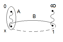
Figure 1: Cycles for the 4-point conformal block

One can directly compute both the periods and the corresponding prepotential to obtain

$$\oint\limits_{A}\Omega_{SW}=\frac{1}{\pi i}K(x),\,\ \ \ \ \oint\limits_{B}\Omega_{SW}=\frac{1}{\pi}K(1-x),\,\ \ \ \ F(a)=\frac{ia^{2}}{2}\frac{K(1-x)}{K(x)}$$ (61)

It is immediate to observe that the rational transformation $z\mapsto 1-z$ permutes the contours $(A,B)\mapsto(-B,A)$, so that one obtains the conjugated prepotential with the variable $x$ replaced with $1-x$. In other words,

$$\boxed{F^{*}(a,x)=F(a,1-x)}$$ (62)

This relation works equally well in the generic case even if the masses or the deformation parameters $\epsilon_{1,2}$ are non-zero. Since the prepotential is directly related to the conformal block, one naturally associates this permutation of contours with the modular transformation $x\to 1-x$ of the prepotential, i.e.

$$\boxed{F\mathop{\longrightarrow}^{M_{\Delta,\Delta^{\prime}}}F^{*}}$$ (63)

This statement allows one to construct the corresponding modular matrix in an explicit way. Indeed, the S-duality transformation that relates the SW prepotential and its conjugated is known to be nothing but the Legendre transformation

$$F^{*}(a,x)=\sup\limits_{b}\Big{(}F(b,x)-ab\Big{)}=F(a,1-x)$$ (64)

This relation can be understood as the leading (semiclassical) approximation to

$$\exp\left\{\frac{2\pi i}{\epsilon_{1}\epsilon_{2}}F^{*}(a)\right\}=\int db\,\exp\left\{\frac{2\pi i}{\epsilon_{1}\epsilon_{2}}ab\right\}\exp\left\{\frac{2\pi i}{\epsilon_{1}\epsilon_{2}}F^{*}(b)\right\}$$ (65)

at small deformation parameters $\epsilon_{1,2}$. In other words, the asymptotic behavior of the modular matrix is

$$M_{a,b}\sim\exp\left\{\frac{2\pi i}{\epsilon_{1}\epsilon_{2}}ab\right\}$$ (66)

4.2 Exactly solvable cases

We are going to consider now the cases when the SW approximation turns out to be almost exact. It happens when the coefficients in the Zamolodchikov recursive formula [24] which are in charge of the ”non-classical” part are equal to zero:

$$B(\Delta_{1},\Delta_{2},\Delta_{3},\Delta_{4};\Delta|x)=\left(e^{\pi i{\cal T}}\right)^{\Delta-\frac{c-1}{24}}x^{\frac{c-1}{24}-\Delta_{1}-\Delta_{2}}(1-x)^{\frac{c-1}{24}-\Delta_{2}-\Delta_{3}}\theta_{3}({\cal T})^{\frac{c-1}{2}-4(\Delta_{1}+\Delta_{2}+\Delta_{3}+\Delta_{4})}\times$$ (67)

$$\times\Big{(}1+H_{non-classical}(\Delta_{1},\Delta_{2},\Delta_{3},\Delta_{4};\Delta|x)\Big{)},\ \ \ \ \ \ \ \ \ \quad{\cal T}=i\frac{K(1-x)}{K(x)}\ \ \ \ \ \ \ \ \$$

This is well-known to be the case for the $SU(2)$ theory with $N_{f}=4$ matter fundamentals with the masses such that $\Delta_{i}=\frac{1}{16}$, $\Delta=\frac{a^{2}}{g^{2}}$ and the deformation parameters such that $c=1$. Then:

$$B\left(a|x\right)=\frac{e^{\frac{\pi i}{g^{2}}{\cal T}a^{2}}}{\left[x(1-x)\right]^{\frac{1}{8}}\theta_{3}({\cal T})}$$ (68)

(69)

$$B\left(a|x\right)=\int\frac{db}{g}\,e^{\frac{2\pi iab}{g^{2}}}B\left(b|1-x\right)$$ (70)

The second exactly solvable case is the $SU(2)$ theory with the adjoint matter field with the adjoint mass and the deformation parameters such that $\Delta_{\mbox{\footnotesize{ext}}}=0$ and $c=1$. This theory corresponds to the toric conformal block (with $\Delta=\frac{a^{2}}{g^{2}}$) and

$$B\left(a|{\cal T}\right)=\frac{e^{\frac{2\pi i}{g^{2}}{\cal T}a^{2}}}{\eta({\cal T})}$$ (71)

(72)

$$B\left(a|{\cal T}\right)=\int\frac{db}{g}\,e^{\frac{4\pi iab}{g^{2}}}B\left(b\left|-\frac{1}{{\cal T}}\right.\right)$$ (73)

in this case.

As one can see, in these both examples the asymptotic form of the modular matrix is exact. In fact, these two cases are basically equivalent due to the correspondence between the one-point conformal block on a torus and a conformal block on a sphere, see [26] and s.6.1.

4.3 Fourier transform from ${\cal U}_{q}(sl_{2})$ algebra

These exact formulas can be compared with those obtained for the Ponsot-Teschner kernel (41). For instance, when the external dimension in the toric conformal block goes to zero, the complicated kernel (41) is drastically simplified. Naively one would expect from eq.(41) and using (43) that, in this case,

$$M=2^{3/2}\int\frac{e^{4\pi ia^{\prime}r}dr}{16\sinh\left(\frac{\pi(a+r)}{\epsilon_{1}}\right)\sinh\left(\frac{\pi(a+r)}{\epsilon_{2}}\right)\sinh\left(\frac{\pi(a-r)}{\epsilon_{1}}\right)\sinh\left(\frac{\pi(a-r)}{\epsilon_{2}}\right)}$$ (74)

In fact, the denominator in the integrand of (41) has double poles, which merge in the limit of $p_{0}\rightarrow i\frac{\epsilon}{2}$, and the integration contour is pinched between these two poles. Hence, one has to deal with this limit more carefully:

$${\cal M}(a,a^{\prime}|0)=\oint\limits_{r=-a}\frac{s(a+r+i\epsilon/2+i\lambda)}{s(a+r-i\epsilon/2-i\lambda)}\frac{e^{4\pi ia^{\prime}r}dr}{4\sinh\left(\frac{\pi(a-r)}{\epsilon_{1}}\right)\sinh\left(\frac{\pi(a-r)}{\epsilon_{2}}\right)}+$$

$$+\oint\limits_{r=a}\frac{s(a-r+i\epsilon/2+i\lambda)}{s(a-r-i\epsilon/2-i\lambda)}\frac{e^{4\pi ia^{\prime}r}dr}{4\sinh\left(\frac{\pi(a+r)}{\epsilon_{1}}\right)\sinh\left(\frac{\pi(a+r)}{\epsilon_{2}}\right)}$$ (75)

Since

$$\frac{s(a+r+i\epsilon/2+i\lambda)}{s(a+r-i\epsilon/2-i\lambda)}=\prod\limits_{m,n\geq 0}\frac{(m+1/2)\epsilon_{1}+(n+1/2)\epsilon_{2}-i(a+r+i\epsilon/2+i\lambda)}{(m+1/2)\epsilon_{1}+(n+1/2)\epsilon_{2}+i(a+r+i\epsilon/2+i\lambda)}\times$$

$$\times\frac{(m+1/2)\epsilon_{1}+(n+1/2)\epsilon_{2}+i(a+r-i\epsilon/2-i\lambda)}{(m+1/2)\epsilon_{1}+(n+1/2)\epsilon_{2}-i(a+r-i\epsilon/2-i\lambda)}=$$

$$=\prod\limits_{m,n\geq 0}\frac{(m+1)\epsilon_{1}+(n+1)\epsilon_{2}-i(a+r+i\lambda)}{m\epsilon_{1}+n\epsilon_{2}+i(a+r+i\lambda)}\frac{(m+1)\epsilon_{1}+(n+1)\epsilon_{2}+i(a+r-i\lambda)}{m\epsilon_{1}+n\epsilon_{2}-i(a+r-i\lambda)}\sim$$

$$\mathop{\sim}_{m,n=0}\ \ \frac{1}{(a+r)^{2}-\lambda^{2}}\ \ \mathop{\sim}_{\lambda\rightarrow 0}\ \ \delta(a+r)$$ (76)

one finally obtains

$${\cal M}(a,a^{\prime}|0)\rightarrow\frac{\sqrt{2}\cos\left(4\pi i\frac{aa^{\prime}}{\epsilon_{1}\epsilon_{2}}\right)}{\mu^{\prime}(a)}$$ (77)

Thus, indeed, in this limit the modular transformation reduces just to the simple Fourier transform as we already saw in s.4.2.

The Fourier transform can be also derived in the limit of $\epsilon_{1,2}\rightarrow 0$. Assume that $\Im\hbox{m}\Big{(}\frac{\epsilon_{1}}{\epsilon_{2}}\Big{)}>0$, then the asymptotics of the quantum dilogarithm has different signs depending on the direction

$$s(z|\epsilon_{1},\epsilon_{2})\sim\left\{\begin{array}[]{c}e^{\frac{\pi i}{2}z^{2}},\quad\mathop{\rm arg}\epsilon_{1}-\frac{\pi}{2}<\mathop{\rm arg}z<\mathop{\rm arg}\epsilon_{2}+\frac{\pi}{2}\\ e^{-\frac{\pi i}{2}z^{2}},\quad\mathop{\rm arg}\epsilon_{2}-\frac{3\pi}{2}<\mathop{\rm arg}z<\mathop{\rm arg}\epsilon_{1}-\frac{\pi}{2}\end{array}\right.$$ (80)

This leads to the limit for the modular kernel for $\epsilon_{1,2}\rightarrow 0$

$$M(a,a_{D})\sim\int dt\exp\left\{\frac{\pi i}{2\epsilon_{1}\epsilon_{2}}\left(2t^{2}-(t-a_{D})^{2}+(t+a_{D})^{2}-(t-a)^{2}+(t+a)^{2}\right)\right\}\sim e^{\frac{2\pi i}{\epsilon_{1}\epsilon_{2}}aa_{D}}$$ (81)

Unfortunately, this approach does not allow one to find the next corrections to the modular matrix, since in the asymptotics $\epsilon_{1,2}\rightarrow 0$ there is only quadratic term in the exponential (80), so further corrections look exponentially small and are not obtained within the asymptotic perturbation theory [27]. At the same time, as we demonstrate in the next section, the actual corrections are not like this (not exponentially small), and it is a question (not answered in the present paper), how (74) should be effectively treated in order to reproduce them.

5 Genus expansion in matrix models and corrections to the modular kernel

5.1 Loop equations

In order to obtain a way to effectively generate manifest formulas for the $S$-duality, we are going to apply the technique of matrix models which, in accordance with the AGT conjecture, describe the conformal blocks and Nekrasov functions, see s.3.2. This technique allows one to calculate the modular kernel, i.e. to construct the $S$-duality transformations iteratively using the matrix model loop equations.

Thus, we consider the multiple integral (53). The standard way to deal with matrix integrals is to construct loop equations for the k-point resolvents [28, 15]

$$r_{k}(\xi_{1},\ldots,\xi_{k})=\left<\sum_{i}{1\over\xi_{1}-z_{i}}\sum_{i}{1\over\xi_{2}-z_{i}}\ \ldots\ \sum_{i}{1\over\xi_{k}-z_{i}}\right>$$ (82)

where the brackets denote the average w.r.t. to the measure (53)

$$\int_{\gamma_{i}}dz_{i}\left(\prod\limits_{j>i}z_{ij}^{2\beta}\right)\prod\limits_{a}(z_{i}-q_{a})^{\frac{2b\alpha_{a}}{g}}$$ (83)

We also use the connected correlators and denote them through $\rho_{k}(\xi_{1},\ldots,\xi_{k})$. For $k=1$ we additionally shift

$$\rho_{1}(z)=\sqrt{\beta}\left(gr_{1}(z)+\sum_{a}{\alpha_{a}\over z-q_{a}}\right)$$ (84)

The loop equations for the unconnected resolvents form the following set of equations

$$\beta r_{k+1}(\zeta,\zeta,x_{1},\ldots,x_{k+1})+(\beta-1)\partial_{\zeta}r_{k}(\zeta,x_{1},\ldots,x_{k-1})+\sum\limits_{a}\frac{2\sqrt{\beta}\alpha_{a}}{g}\frac{r_{k}(\zeta,x_{1},\ldots,x_{k-1})-r_{k}(q_{a},x_{1},\ldots,x_{k-1})}{\zeta-q_{a}}+$$

$$+\sum_{j}\partial_{x_{j}}\frac{r_{k-1}(x_{1},\ldots,x_{k-1})-\left.r_{k-1}(x_{1},\ldots,x_{k-1})\right|_{x_{j}=\zeta}}{x_{j}-\zeta}=0$$ (85)

One can reformulate it in terms of the connected resolvents which admits ”the genus expansion” in powers of the coupling constant $g$. These equations are a bit more involved. The first few of them are

$$g^{2}\beta\rho_{2}(z)+g\left(\sqrt{\beta}-\frac{1}{\sqrt{\beta}}\right)\left(\partial\rho_{1}(z)+\sqrt{\beta}\sum\limits_{a}\frac{\alpha_{a}}{(z-q_{a})^{2}}\right)+\rho_{1}^{2}(z)-\sum\limits_{a}\frac{\partial_{q_{a}}{\cal F}}{z-q_{a}}-\beta\left(\sum\limits_{a}\frac{\alpha_{a}}{z-q_{a}}\right)^{2}=0$$

$$g^{2}\beta\rho_{3}(z)+\frac{1}{2}g(\beta-1)\partial\rho_{2}(z)+2\rho_{1}(z)\rho_{2}(z)-\sum\limits_{a}\frac{\partial_{q_{a}}\rho_{1}(z)}{z-q_{a}}+\frac{1}{2}\partial^{2}\rho_{1}(z)=0$$

$$2\rho_{1}(z)\rho_{3}(z)+2\rho_{2}^{2}(z)-\sum\limits_{a}\frac{\partial_{q_{a}}\rho_{2}(z)}{z-q_{a}}+(\hat{L}\rho_{2})(z)=0$$

$$2\partial^{2}\rho_{1}(z)\rho_{2}(z)+2\partial\rho_{1}(z)\partial\rho_{2}(z)+2\rho_{1}(z)(\hat{L}\rho_{2})(z)-2\sum\limits_{a}\frac{\partial_{q_{a}}\rho_{1}(z)}{(z-q_{a})^{3}}+\frac{1}{12}\partial^{4}\rho_{1}(z)=0$$ (86)

where

$$(\hat{L}\rho_{2})(z)=\left.\partial_{z}\partial_{w}\rho_{2}(z,w)\right|_{w=z}$$ (87)

and ${\cal F}$ differs from $F$ by omitting the normalization factor $\prod_{a<b}(q_{q}-q_{b})^{2\alpha_{a}\alpha_{b}/g}$ from (53).

The matrix model ($\beta$-ensemble) partition function can be calculated using the SW equations (56) for its logarithm. The complex spectral curve is determined from the genus zero contribution to the first equation of (86) which involves only the 1-point resolvent $\rho_{1}^{(0)}(z)$ (84)

$$y^{2}(z)=\rho_{1}^{(0)}(z)^{2}=\sum\limits_{a}\frac{\partial_{q_{a}}{\cal F}}{z-q_{a}}+\beta\left(\sum\limits_{a}\frac{\alpha_{a}}{z-q_{a}}\right)^{2}$$ (88)

while the differential is

$$\Omega_{g,\beta}=\rho_{1}(z)dz$$ (89)

5.2 Modular kernel construction

Similarly to the expansion of the prepotential into powers of the string coupling constant $g$, one can perform this expansion for the modular matrix. Thus, we assume the following expansions

$$F(a,x)=\sum\limits_{k=0}^{\infty}g^{2k}F_{k}(a,x)$$ (90)

$$M(a,b)=\exp\left(\frac{2\pi iab}{g^{2}}+\sum\limits_{k=0}^{\infty}g^{2k}\mathfrak{m}_{k}(a,b)\right)$$ (91)

which should be inserted into the definition of the modular kernel $M(a,b)$

$$e^{\frac{2\pi i}{g^{2}}F(b,1-x)}=\int\frac{da}{g}M(a,b)e^{\frac{2\pi i}{g^{2}}F(a,x)}$$ (92)

Then, a simple computation leads to the following relation

$$F(b,1-x)=\left(F(a_{0},x)+a_{0}b\right)+g^{2}\left(\mathfrak{m}_{0}(a_{0},b)+F_{1}(a_{0}|x)-\frac{1}{4\pi i}\log F_{0}^{\prime\prime}(a_{0}|x)\right)+$$

$$+g^{4}\left(\mathfrak{m}_{1}(a_{0},b)+F_{2}(a_{0}|x)+\frac{i}{4\pi}\frac{F_{1}^{\prime\prime}(a_{0}|x)}{F_{0}^{\prime\prime}(a_{0}|x)}+\frac{i}{4\pi}\frac{\mathfrak{m}_{0}^{\prime\prime}(a_{0},b)}{F_{0}^{\prime\prime}(a_{0}|x)}-\frac{1}{2}\frac{(\mathfrak{m}_{0}^{\prime}(a_{0},b))^{2}}{F_{0}^{\prime\prime}(a_{0}|x)}-\frac{1}{2}\frac{(F_{1}^{\prime}(a_{0}|x))^{2}}{F_{0}^{\prime\prime}(a_{0}|x)}+\right.$$

$$\left.-\frac{\mathfrak{m}_{0}^{\prime}(a_{0},b)F_{1}^{\prime}(a_{0}|x)}{F_{0}^{\prime\prime}(a_{0}|x)}-\frac{1}{32\pi^{2}}\frac{F_{0}^{(IV)}(a_{0}|x)}{(F_{0}^{\prime\prime}(a_{0}|x))^{2}}-\frac{i}{4\pi}\frac{F_{0}^{\prime\prime\prime}(a_{0}|x)F_{1}^{\prime}(a_{0}|x)}{(F_{0}^{\prime\prime}(a_{0}|x))^{2}}+\frac{5}{96\pi^{2}}\frac{(F_{0}^{\prime\prime\prime}(a_{0}|x))^{2}}{(F_{0}^{\prime\prime}(a_{0}|x))^{3}}\right)+\ldots,$$ (93)

where $a_{0}$ is determined from the equation $F_{0}^{\prime}(a_{0}|x)+b=0$ and the prime means the derivative w.r.t. $a_{0}$. This relation can be also viewed as defining the function $x(a,b)$ in an implicit way

$$F_{0}^{\prime}(a|x(a,b))=-b$$ (94)

Using this formula, one can eliminate the $x$-dependence from the modular kernel. For instance, in the first order one has

$$\mathfrak{m}_{0}(a,b)=F_{1}(b,1-x(a,b))-F_{1}(a|x(a,b))+\frac{1}{4\pi i}\log F_{0}^{\prime\prime}(a|x(a,b))$$ (95)

5.3 First few terms of expansion

Here we present some explicit expressions for the first few terms of expansion of the prepotential calculated on the lines of s.5.1. Then, following s.5.2, we find the corresponding genus expansion of the modular kernel.

Example 1: $\epsilon_{1}=-\epsilon_{2}=g$ or $\beta=1$ with $\mu_{1}=2tm_{1},\mu_{2,4}=0,\mu_{3}=2tm_{3}$.

In this case, the prepotential has the following expansion

$$F(\mu_{1}=2tm_{1},\mu_{2}=0,\mu_{3}=2tm_{3},\mu_{4}=0|x)=\sum\limits_{k,m=0}^{\infty}I_{k,2m}(x)g^{2k}t^{2m}$$ (96)

Several first terms in this expansion are given by the following expressions

$$I_{00}=-\frac{\pi a^{2}K(1-x)}{K(x)}$$ (97)

$$I_{02}=2(m_{1}^{2}+m_{3}^{2})\log a$$ (98)

$$I_{04}=-\frac{2(m_{1}^{4}+m_{3}^{4})}{3\pi^{2}a^{2}}\left((x-2)K(x)+3E(x)\right)-\frac{4m_{1}^{2}m_{3}^{2}}{\pi^{2}a^{2}}K(x)\left((x-1)K(x)+E(x)\right)$$ (99)

$$I_{10}=-\frac{1}{2}\log a$$ (100)

$$I_{12}=\frac{2(m_{1}^{2}+m_{3}^{2})}{3\pi^{2}a^{2}}K(x)\left((x-2)K(x)+E(x)\right)$$ (101)

$$I_{14}=\frac{4(m_{1}^{4}+m_{3}^{4})}{3\pi^{2}a^{4}}K^{2}(x)\left[(x^{2}-3x+3)K^{2}(x)+4(x-2)K(x)E(x)+6E^{2}(x)\right]+$$

$$+\frac{8m_{1}^{2}m_{3}^{2}}{3\pi^{4}a^{4}}\left[(3x^{2}-7x+4)K^{2}(x)+2(4x-5)K(x)E(x)+6E^{2}(x)\right]$$ (102)

$$I_{20}=-\frac{K(x)}{8\pi^{2}a^{2}}\left((x-2)K(x)-3E(x)\right)$$ (103)

$$I_{22}=-\frac{m_{1}^{2}+m_{3}^{2}}{60\pi^{4}a^{4}}K^{2}(x)\left((48x^{2}-143x+143)K^{2}(x)+190(x-2)K(x)E(x)+285E^{2}(x)\right)$$ (104)

$$I_{24}=-\frac{K^{3}(x)(m_{1}^{4}+m_{3}^{4})}{90\pi^{6}a^{6}}\left(-1646K^{3}(x)+4350E^{3}(x)+2469xK^{3}(x)-8700K(x)E^{2}(x)+6476K^{2}(x)E(x)-\right.$$

$$\left.-1783K^{3}(x)^{3}x^{2}+480x^{3}K^{3}(x)+4350K(x)E^{2}(x)x+2126K^{2}(x)x^{2}E(x)-6476K^{2}(x)xE(x)\right)-$$

$$-\frac{K^{3}(x)m_{1}^{2}m_{3}^{2}}{45\pi^{6}a^{6}}\left(-1646K^{3}(x)+4350E^{3}(x)+2469K^{3}(x)x-8700K(x)E^{2}(x)+6476K^{2}(x)E(x)-1783K^{3}(x)x^{2}+\right.$$

$$\left.+480x^{3}K^{3}(x)+4350K(x)E^{2}(x)x+2126K^{2}(x)x^{2}E(x)-6476K^{2}(x)E(x)x\right)$$ (105)

Surprisingly, in this case of only two zero masses the modular matrix does not seem to differ from the Fourier transform:

$$\boxed{e^{\frac{1}{g^{2}}F(x|a)}=\int\frac{db}{g}e^{\frac{2\pi iab}{g^{2}}+{\cal O}(t^{6},g^{4})}e^{\frac{1}{g^{2}}F(1-x|b)}}$$ (106)

Even more surprisingly, this seems to remain true for arbitrary masses: corrections are absent whenever $\beta=1$ (though we do not possess yet a complete evidence in favor of this conjecture).

Example 2: Double deformation $\beta\neq 1$ with $\mu_{1}=\mu_{2}=-\mu_{3}=-\mu_{4}=\epsilon/2$.

In the case of the arbitrary double deformation the modular kernel is no longer the Fourier transform. We demonstrate this in the simplest case of masses $\mu_{1}=\mu_{2}=-\mu_{3}=-\mu_{4}=\epsilon/2$. Then, the prepotential is

$$F=-\frac{\pi a^{2}K(1-x)}{K(x)}+\frac{g^{2}}{2}\left(3\beta-7+\frac{3}{\beta}\right)\log a-$$

$$-\frac{g^{4}}{8a^{2}}\frac{\left(3\beta-7+\frac{3}{\beta}\right)\left(\beta-3+\frac{1}{\beta}\right)}{\pi^{2}}K(x)\left((x-2)K(x)+3E(x)\right)+\ldots$$ (107)

The modular matrix in this case reads

$$\boxed{M(a,b)=\exp\left(\frac{2\pi iab}{g^{2}}+\frac{3(\beta-1)^{2}}{2\beta}\log\frac{a}{b}-\frac{3ig^{2}}{16\pi\beta^{2}}\frac{(\beta-3)(3\beta-1)(\beta-1)^{2}}{ab}+\ldots\right)}$$ (108)

Thus, for $\beta\neq 1$ corrections to the Fourier transform are non-vanishing.

6 $S$-duality in the NS limit: comments and remarks

In the previous section we used the matrix model technique in order to manifestly construct the $S$-duality kernel as a series in powers of $\beta-1$, i.e. around the line $\beta=1$. In this section we briefly discuss peculiarities of another important line $\epsilon_{2}=0$ (the NS limit [29]) which are essential for further studies, since in the NS limit the modular properties are much simpler than in the generic case, and there is a hope to understand them in much more details. This limit is also interesting from the point of view of integrable systems, because there the remaining $\epsilon_{1}$ can be treated as a quantization parameter.

6.1 Modular transformation on torus

So far using the matrix model technique we discussed how to obtain the $S$-duality kernel of conformal blocks on a sphere. One can similarly deal with the conformal blocks on a torus, though the matrix model is somewhat more involved [30]. In practice, it is simpler to use an equivalence of the one-point toric conformal block and a special four-point spherical conformal block [26]. However, in [26] this equivalence is established through a sophisticated recursion procedure which is still not very well understood. Here we describe this equivalence in a much more explicit way, but only in the limit $\epsilon_{2}\rightarrow 0$, i.e. when there is an underlying quantum integrable system (the elliptic Calogero model [31, 32, 33]) and a ”quantized” SW curve. In order to completely describe the conformal block in this limit, one has to insert an additional field, degenerate at the second level [34], and consider the equation for the conformal block that emerge after this [1]. This Schrödinger-Baxter equation is exactly what one calls the ”quantized” SW curve, and the logarithmic derivative of solution of this equation is the SW differential. Using this SW data, one constructs the Nekrasov function in the NS limit, $\epsilon_{2}\to 0$.

Thus, the conformal blocks to compare are the 5-point spherical block and the toric 2-point block, both with one of the fields degenerate at the second level and the properly adjusted intermediate dimensions [35]. We demonstrate that the differential equation for the toric block reduces to a particular case of the spherical block differential equation. The original four-point and one-point conformal blocks can afterwards be extracted from the asymptotics of the solutions by a procedure presented in [35].

In the limit of $\epsilon_{2}\to 0$, the differential equation for the toric conformal block is [35]

$$\left\{2\pi i\frac{\partial}{\partial\tau_{0}}-4\frac{\epsilon_{1}}{\epsilon_{2}}\left[\sqrt{(X-e_{1})(X-e_{2})(X-e_{3})}\partial_{X}\right]^{2}+\frac{\mu(\epsilon_{1}-\mu)}{\epsilon_{1}\epsilon_{2}}X\right\}\Psi\Big{(}\tau_{0},X\Big{)}=0$$ (109)

where, as compared with [35, eq.(36)], we left only the terms essential in the limit $\epsilon_{2}\rightarrow 0$ and introduced the variable $X=\wp(z|\tau_{0})$, i.e. $z=\frac{1}{2}\int\limits_{X}^{\infty}\frac{ds}{\sqrt{(s-e_{1})(s-e_{2})(s-e_{3})}}$, with

$$e_{1}=\frac{\pi^{2}}{3}(2-x)\theta_{3}^{4}(\tau_{0}),\quad e_{2}=-\frac{\pi^{2}}{3}(1+x)\theta_{3}^{4}(\tau_{0}),\quad e_{3}=-\frac{\pi^{2}}{3}(1-2x)\theta_{3}^{4}(\tau_{0}),\quad x=\frac{\theta_{2}^{4}(\tau_{0})}{\theta_{3}^{4}(\tau_{0})}$$ (110)

The external dimension $\Delta=\frac{\mu(\epsilon_{1}-\mu)}{\epsilon_{1}\epsilon_{2}}$ parameterizes the mass $\mu$ of the adjoint matter hypermultiplet (adding this hypermultiplet corresponds to the toric conformal block in the AGT framework).

Now, change of the variable $X=e_{2}-t(e_{1}-e_{2})$ leads to the equation

$$\left\{\frac{1}{2}x(x-1)\partial_{x}+t(t-1)(t-x)\left[\partial_{t}^{2}-\frac{1}{2}\left(\frac{1}{t}+\frac{1}{t-1}+\frac{1}{t-x}\right)\right]+\frac{\mu(\epsilon_{1}-\mu)}{4\epsilon_{1}\epsilon_{2}}\left(t-\frac{1}{3}(1+x)\right)\right\}\Psi(x,t)=0$$ (111)

By rescaling the wave function $\tilde{\Psi}(t)=\left[t(t-1)(t-x)\right]^{-\frac{1}{4}}\Psi(t)$, one can eliminate the term linear in $\partial_{t}$, up to the order $\mathcal{O}(\epsilon_{2}^{0})$. This procedure redefines the SW integral, with the intermediate dimension $\Delta_{\alpha}=\frac{\alpha(\epsilon-\alpha)}{\epsilon_{1}\epsilon_{2}}$), in accordance with

$$\frac{\epsilon_{1}}{2\pi i}\oint_{A}d_{t}\log\tilde{\Psi}=\frac{\epsilon_{1}}{2\pi i}\oint_{A}d_{t}\log\Psi-\frac{\epsilon_{1}}{2}=\alpha-\frac{\epsilon_{1}}{2}=a$$

This equation coincides with that for the spherical conformal block [35, eqs.(85)-(86)] in the limit $\epsilon_{2}\rightarrow 0$ provided one rescales the modular parameter $\tau_{0}\rightarrow 2\tau_{0}$ and the wave function $\psi=\tilde{\Psi}\left[x(x-1)\right]^{-\frac{\Delta}{12}}$:

$$\left[x(x-1)\partial_{x}-\frac{\epsilon_{1}}{\epsilon_{2}}t(t-1)(t-x)\partial_{t}^{2}-\frac{\mu(\epsilon_{1}-\mu)}{4\epsilon_{1}\epsilon_{2}}(t-x)\right]\psi(x,t)=0$$ (112)

Since the wave functions are the same for toric and spherical cases, the same is true for the conformal blocks. Thus, we reproduce the answer of [26], but only in the limit $\epsilon_{2}\rightarrow 0$

$$Z_{{\rm sphere}}\left(\Delta_{1,2,3}=0,\Delta_{4}=\frac{\Delta}{4}\Big{|}x=\frac{\theta_{2}^{4}(2\tau_{0})}{\theta_{3}^{4}(2\tau_{0})}\right)=\eta^{-2\Delta}(\tau_{0})\left(\frac{\theta_{3}^{8}(2\tau_{0})}{\theta_{2}^{4}(2\tau_{0})\theta_{4}^{4}(2\tau_{0})}\right)^{\frac{\Delta}{12}}Z_{{\rm torus}}(\Delta|\tau_{0})$$ (113)

This means that the toric conformal block has the same transformation properties as the spherical one, its modular/$S$-duality operator in the limit $\epsilon_{1,2}\to 0$ being

$$M(a,a^{\prime})=e^{\frac{4\pi iaa^{\prime}}{\epsilon_{1}\epsilon_{2}}}$$ (114)

Note that we made the rescaling $\tau_{0}\rightarrow 2\tau_{0}$, thus this formula is in accordance with the results of [3]. In sect.4.2 we already encountered an explicit application of this result.

6.2 $S$-transformation of effective coupling constants

Throughout the paper we mostly concentrated on the modular kernel for the transformation $x\to 1-x$, which turns to resemble the Fourier transform. One may also ask how the effective coupling constant behaves under this transformation.

As we discussed above, the $S$-duality transformation of an effective charge matrix defined as $||{\cal T}_{\epsilon_{1},\epsilon_{2}}||_{i,j}=\frac{\partial^{2}F_{\epsilon_{1},\epsilon_{2}}}{\partial a_{i}\partial a_{j}}$, has the simple form in the SW case:

$$\hat{S}({\cal T}_{0,0})=-({\cal T}_{0,0})^{-1}$$ (115)

In fact, it is preserved in the once deformed case too:

$$\hat{S}({\cal T}_{\epsilon_{1},0})=-({\cal T}_{\epsilon_{1},0})^{-1}$$ (116)

The reason that this property survives the deformation is that in this case there still exists the closed (Baxter or Schrödinger) equation for the SW differential so that one can immediately construct the Bohr-Sommerfeld integrals to obtain the SW prepotential, and the SW differential remains intact under duality transformations. However, this is no longer the case when the both deformations are switched on. Indeed, in this case the SW differential is determined only from the loop equations involving all multi-point resolvents and

$$\hat{S}({\cal T}_{\epsilon_{1},\epsilon_{2}})\neq-({\cal T}_{\epsilon_{1},\epsilon_{2}})^{-1}$$ (117)

There is the following technical reason for this. Consider the space of coupling constants $x=e^{2\pi i\tau_{0}}$ and the fiber bundle of the Riemann surfaces over this space $u(x)=\langle{\rm Tr}\,\phi^{2}\rangle$. With this bundle, one can construct the A- and B-periods of the 1-resolvent: $a(x)=\langle\phi\rangle$, $b(x)$. As soon as the SW differential or the equation for it in the once deformed case depends only on $u(x)$, but not on its derivatives, one can locally interchange the cycles at some point $x_{0}$, i.e. just change the value of $a(x)$ at this point $x=x_{0}$, and it is completely independent on the value of $a(x)$ at any other point $x$. This property is broken, however, by the matrix model corrections, since then the derivatives of $u(x)$ manifestly enter the differential (and the equations for it). On the other hand, we fix $a(x)=const$, $b(x)$ is a non-trivial function and one can no longer permute the cycles locally at some $x_{0}$. To put it differently, in order to completely fix the multi-resolvents in matrix model, one has to impose some condition on their A-periods: for instance, to require that they vanish. This manifestly breaks the symmetry under permutations of the A- and B-cycles, see Fig.2.

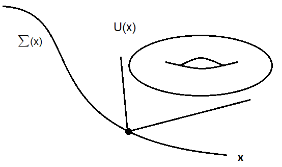
Figure 2: Family of effective tori defining the matrix model partition function

6.3 On the full duality group

We discussed so far only the $S$-transformation from the duality group. One may ask what is the full duality group, i.e. when one adds the generator of the $T$-transformation. This question was addressed in detail in numerous papers [7, 8, 9, 10], still a few short remarks deserve mentioning.

Note that so far we considered different groups of transformations. First of all, it is the group of modular transformations of the conformal blocks. It is related by the AGT relations with the $S$-duality group. The modular transformations are induced by the third group, which relates different possibilities to arrange the brackets in the tensor products. This group sometimes coincides with the group of permutations of points, as we discuss in this section below.

6.3.1 $SL(2,\mathbb{Z})$ and Racah identities

We start with the case of $SU(2)$ gauge group, i.e. with the four-point conformal block. Note that the associativity of the operator algebra implies an essential property of the Racah-Wiegner coefficients: considering multiple products of representations and rearranging brackets in different ways, one arrives at commutative diagrams. One of these is

$$\begin{CD}(T_{1}\otimes T_{2})\otimes T_{3}@>{\hat{T}}>{}>(T_{2}\otimes T_{1})\otimes T_{3}@>{\hat{R}}>{}>T_{2}\otimes(T_{1}\otimes T_{3})\\ @V{}V{\hat{R}}V@V{}V{\hat{F}}V\\ T_{1}\otimes(T_{2}\otimes T_{3})@<{\hat{T}}<{}<T_{1}\otimes(T_{3}\otimes T_{2})@<{\hat{R}}<{}<(T_{1}\otimes T_{3})\otimes T_{2}\end{CD}$$ (118)

which imposes a nontrivial restriction $\hat{T}\hat{R}\hat{F}\hat{R}\hat{T}=\hat{R}$ on the modular kernel. For the modular and $S$-duality transformation with generators $\hat{S}$ and $\hat{T}$ one has $\hat{R}=\hat{T}\hat{S}$, $\hat{F}=\hat{1}$, and the Racah relation is equivalent to $(\hat{T}\hat{S})^{3}=1$. Along with $\hat{S}^{2}=1$ this implies that these transformations generate $SL(2,\mathbb{Z})$.

As we discussed in the previous subsection, one can realize these generators in the NS limit either in terms of the effective coupling constant ${\cal T}$ on the gauge theory side ($S$-duality) as

$$\hat{S}:\quad{\cal T}\mapsto-1/{\cal T},\quad\hat{T}:\quad{\cal T}\mapsto{\cal T}+1,$$ (119)

or in terms of the double ratio (bare coupling constant in the gauge terms) of four points on the CFT side (modular transformation) as

$$\hat{\bar{S}}:\quad x\mapsto 1-x,\quad\hat{\bar{T}}:\quad x\mapsto\frac{x}{x-1}$$ (120)

In the first representation, one obtains only two relations for the generators: $\hat{S}^{2}=1$ and $(\hat{T}\hat{S})^{3}=1$, while in the second one there is the additional restriction $\hat{\bar{T}}^{2}=1$, i.e. the generators, in this case, form a finite group of permutations $S_{3}$. This seeming contradiction with the AGT relation is resolved once one notice that the main object of our interest, the conformal block also does not obey the relation $\hat{T}^{2}=1$ because of the singular behaviour: $B\sim x^{\Delta-\Delta_{1}-\Delta_{2}}$, $x\rightarrow 0$. As a result, the action of $\hat{T}^{2}$ which carries the point $q$ around zero gives rise to a non-trivial monodromy factor, thus, the conformal block provides the representation of $SL(2,\mathbb{Z})$, not of $S_{3}$.

6.3.2 Multi-point conformal blocks

This difference between the permutation and duality groups becomes more profound for multi-point conformal blocks. Indeed, in this case not all possible modular transformations (i.e. all possible ways to place brackets in the tensor products) can be associated with permutations of points. This happens starting from the six-point conformal block. In the case of the five-point conformal block this is still possible, and the modular transformations can be described by the $S_{4}$ group of permutations. The duality group in this case also has nothing to do with the permutation group. The five-point conformal block described theory with the gauge group $SU(2)\times SU(2)$, however, the duality group is not a direct product of two $SL(2,\mathbb{Z})$, see the detailed discussion in [10]. It is done there for SW theory, i.e. for $\epsilon_{1},\epsilon_{2}=0$, however, it is enough in this case, though one can definitely repeat the matrix model calculations for arbitrary $\epsilon_{1}$ and $\epsilon_{2}$.

The S-duality group contains two $SL(2,\mathbb{Z})$ subgroups and an additional generator mixing them, i.e. one can totally extract five generators: $\hat{S}_{1,2}$, $\hat{T}_{1,2}$ and the mixing generator $\hat{Q}$. As previously, one can construct the Racah relation, which in this case reads

$$\hat{R}_{1}\hat{T}_{1}\hat{R}_{2}\hat{R}_{1}=\hat{Q}\hat{R}_{1}\hat{R}_{2}$$ (121)

with the Racah coefficients given by $\hat{R}_{1,2}=\hat{T}_{1}\hat{T}_{2}\hat{S}_{1,2}$. Since the $S$-duality group contains $SL(2,\mathbb{Z})$ subgroups, the relation $\left(\hat{S}\hat{T}\right)^{3}=1$ still holds.

As we mentioned, beginning with the six-point case the modular transformations are not reduced to permutations of points. The reason is that the new diagram emerges, and one has to describe within the modular transformation the map

$$\begin{picture}(50.0,14.0)\put(0.0,0.0){\line(1,0){50.0}} \put(10.0,0.0){\line(0,1){10.0}} \put(20.0,0.0){\line(0,1){10.0}} \put(30.0,0.0){\line(0,1){10.0}} \put(40.0,0.0){\line(0,1){10.0}} \put(1.0,2.0){\makebox(0.0,0.0)[cc]{$0,\Delta_{1}$}} \put(7.0,12.0){\makebox(0.0,0.0)[cc]{$x_{1},\Delta_{2}$}} \put(17.0,12.0){\makebox(0.0,0.0)[cc]{$x_{2},\Delta_{3}$}} \put(27.0,12.0){\makebox(0.0,0.0)[cc]{$x_{3},\Delta_{4}$}} \put(37.0,12.0){\makebox(0.0,0.0)[cc]{$1,\Delta_{5}$}} \put(50.0,2.0){\makebox(0.0,0.0)[cc]{$\infty,\Delta_{6}$}} \end{picture}\qquad\longrightarrow\qquad\begin{picture}(50.0,14.0)\put(0.0,0.0){\line(1,0){50.0}} \put(10.0,0.0){\line(0,1){10.0}} \put(25.0,0.0){\line(0,1){5.0}} \put(25.0,5.0){\line(1,1){7.0}} \put(25.0,5.0){\line(-1,1){7.0}} \put(40.0,0.0){\line(0,1){10.0}} \put(1.0,2.0){\makebox(0.0,0.0)[cc]{$0,\Delta_{1}$}} \put(7.0,12.0){\makebox(0.0,0.0)[cc]{$x_{1},\Delta_{2}$}} \put(17.0,14.0){\makebox(0.0,0.0)[cc]{$x_{2},\Delta_{3}$}} \put(33.0,14.0){\makebox(0.0,0.0)[cc]{$x_{3},\Delta_{4}$}} \put(43.0,12.0){\makebox(0.0,0.0)[cc]{$1,\Delta_{5}$}} \put(50.0,2.0){\makebox(0.0,0.0)[cc]{$\infty,\Delta_{6}$}} \end{picture}$$

This implies that the modular and $S$-duality groups are different for these theories: this transformation can not be described within the framework of the same SYM theory with modified parameters. This issue requires further efforts to be understood.

7 Conclusion

In this paper, we reviewed the problem of constructing the fusion coefficients in $2d$ conformal field theory from the point of view of the AGT conjecture. We provided some explicit formulas relating the modular map of the conformal blocks to the $S$-duality map of the $\Omega$-background-deformed prepotential or of the Nekrasov partition functions. We demonstrated that $S$-duality transformation is actually the Fourier transform at $\beta=1$, but acquires non-trivial corrections for $\beta\neq 1$. These corrections can be found order-by-order from the Virasoro constraints (loop equations) for the ”conformal” $\beta$-ensemble (i.e. with logarithmic potential) of [13, 14].

Still more effort is needed to reproduce this result from the ${\cal U}_{q}(sl_{2})$-algebra consideration by B.Ponsot and J.Teschner. A generalization to multi-point conformal blocks, deformed Virasoro algebras and ${\cal W}_{N}$-algebras are also open problems.

References

• [1] A.Belavin, A.Polyakov, A.Zamolodchikov, Nucl.Phys., B241 (1984) 333-380;
A.Zamolodchikov and Al.Zamolodchikov, Conformal field theory and critical phenomena in 2d systems, 2009, 168 p. (in Russian)
• [2] N.Vilenkin and A.Klymik, Representation of Lie groups and Special Functions, Volume 3, Mathematics and its applications, Kluwer academic publisher, 1993;
P.Golod and A.Klimyk, Mathematical Foundations of Symmetry Theory, Naukova Dumka Publishers, Kyiv, 1992 (in Ukrainian)
• [3] B.Ponsot and J.Teschner, hep-th/9911110; Commun.Math.Phys. 224 (2001) 613-655, math/0007097;
J. Teschner, Int.J.Mod.Phys. A19S2 (2004) 436-458, hep-th/0303150; Contribution to 14th International Congress on Mathematical Physics (ICMP 2003), hep-th/0308031
• [4] L.Alday, D.Gaiotto and Y.Tachikawa, Lett.Math.Phys. 91 (2010) 167-197, arXiv:0906.3219
• [5] N.Wyllard, JHEP 0911 (2009) 002, arXiv:0907.2189;
A.Mironov and A.Morozov, Phys.Lett. B680 (2009) 188-194, arXiv:0908.2190; Nucl.Phys. B825 (2009) 1-37, arXiv:0908.2569
• [6] C.Montonen and D.Olive, Phys.Lett. B72 (1977) 117;
P.Goddard, J.Nuyts and D.Olive, Nucl.Phys. B125 (1977) 1;
E.Witten and D.Olive, Phys.Lett. B78 (1978) 97;
H.Osborn, Phys.Lett. B83 (1979) 321
• [7] N.Seiberg and E.Witten, Nucl.Phys. B426 (1994) 19-52, hep-th/9407087
• [8] N.Seiberg and E.Witten, Nucl.Phys., B431 (1994) 484-550, hep-th/9408099
• [9] A.Hanany and Y.Oz, Nucl.Phys. B452 (1995) 283-312, hep-th/9505075;
P.Argyres, M.Plesser and A.Shapere, Phys.Rev.Lett. 75 (1995) 1699-1702, hep-th/9505100;
J.Minahan and D.Nemeschansky, Nucl.Phys. B464 (1996) 3, hep-th/9507032; Nucl.Phys. B468 (1996) 72, hep-th/9601059;
O.Aharony and S.Yankielowicz, Nucl.Phys. B473 (1996) 93, hep-th/9601011;
P.Argyres, hep-th/9706095; hep-th/9705076;
J.Minahan, Nucl.Phys. B537 (1999) 243-259,hep-th/9806246
• [10] P.Argyres and A.Buchel, JHEP 9911 (1999) 014, hep-th/9910125
• [11] N.Nekrasov, Adv.Theor.Math.Phys. 7 (2004) 831-864, hep-th/0206161;
N.Nekrasov and A.Okounkov, hep-th/0306238
• [12] N.Nekrasov and E.Witten, JHEP 1009 (2010) 092, arXiv:1002.0888
• [13] R.Dijkgraaf and C.Vafa, arXiv:0909.2453;
H.Itoyama, K.Maruyoshi and T.Oota, Prog.Theor.Phys. 123 (2010) 957-987, arXiv:0911.4244;
T.Eguchi and K.Maruyoshi, arXiv:0911.4797; arXiv:1006.0828;
R.Schiappa and N.Wyllard, arXiv:0911.5337
• [14] A.Mironov, A.Morozov and Sh.Shakirov, JHEP 02 (2010) 030, arXiv:0911.5721; Int.J.Mod.Phys. A25 (2010) 3173-3207, arXiv:1001.0563; JHEP 1103 (2011) 102, arXiv:1011.3481;
A.Mironov, Al.Morozov and And.Morozov, Nucl.Phys. B843 (2011) 534-557, arXiv:1003.5752
• [15] A.Alexandrov, A.Mironov and A.Morozov, Int.J.Mod.Phys. A19 (2004) 4127, hep-th/0310113; Teor.Mat.Fiz. 150 (2007) 179-192, hep-th/0605171; Physica D235 (2007) 126-167, hep-th/0608228; JHEP 12 (2009) 053, arXiv:0906.3305;
A.Alexandrov, A.Mironov, A.Morozov, P.Putrov, Int.J.Mod.Phys. A24 (2009) 4939-4998, arXiv:0811.2825;
B.Eynard, JHEP 0411 (2004) 031, hep-th/0407261;
L.Chekhov and B.Eynard, JHEP 0603 (2006) 014, hep-th/0504116; JHEP 0612 (2006) 026, math-ph/0604014;
B.Eynard and N.Orantin, math-ph/0702045;
N.Orantin, arXiv:0808.0635
• [16] R.K.Kaul and T.R.Govindarajan, Nucl.Phys. B380 (1992) 293-336, hep-th/9111063;
P.Ramadevi, T.R.Govindarajan and R.K.Kaul, Nucl.Phys. B402 (1993) 548-566, hep-th/9212110; Nucl.Phys. B422 (1994) 291-306, hep-th/9312215;
Zodinmawia and P.Ramadevi, arXiv:1107.3918;
A.Mironov, A.Morozov and And.Morozov, arXiv:1112.5754; JHEP 03 (2012) 034, arXiv:1112.2654;
H.Itoyama, A.Mironov, A.Morozov and An.Morozov, arXiv:1204.4785
• [17] D. Gaiotto, G. Moore, A. Neitzke, arXiv:0907.3987;
T. Dimofte, S. Gukov, Y. Soibelman, Lett.Math.Phys. 95 (2011) 1-25, arXiv:0912.1346;
T.Dimofte, S.Gukov and L.Hollands, arXiv:1006.0977;
Yu.Terashima and M.Yamazaki, arXiv:1103.5748;
D.Galakhov, A.Mironov, A.Morozov and A.Smirnov, arXiv:1104.2589
• [18] G.Moore and N.Seiberg, Commun.Math.Phys. 123 (1989) 177-254
• [19] T.Shintani, J. Fac. Sci. Univ. Tokyo, Sect. 1A 24 (1977) 167-199;
N.Kurokawa, Proc. Japan Acad. A67 (1991) 61-64; Proc. Japan Acad. A68 (1992) 256-260; Adv. Studies Pure Math. 21 (1992) 219-226;
L.Faddeev and R.Kashaev, Mod.Phys.Lett. A9 (1994) 427-434, hep-th/9310070;
L.Faddeev, Lett. Math. Phys. 34 (1995) 249; hep-th/9504111; math.qa/9912078;
S.Sergeev, V.Bazhanov, H.Boos, V.Mangazeev and Yu.Stroganov, IHEP-95-129, 1995;
M.Jimbo and T.Miwa, J.Phys. A29 (1996) 2923-2958; hep-th/9601135;
S. Ruijsenaars, J. Math. Phys. 38 (1997) 1069–1146;
R. Kashaev, Lett.Math.Phys. 43 (1998) 105-115
• [20] E.W.Barnes, Proc. London Math. Soc. 31 (1899) 358-381; Phil. Trans. Roy. Soc. A196 (1901) 265-387; Trans. Cambr. Phil. Soc. 19 (1904) 374-425
• [21] G.Moore, N.Nekrasov and S.Shatashvili, Nucl.Phys. B534 (1998) 549-611, hep-th/9711108; hep-th/9801061;
A.Losev, N.Nekrasov and S.Shatashvili, Commun.Math.Phys. 209 (2000) 97-121, hep-th/9712241; ibid. 77-95, hep-th/9803265
• [22] A.Marshakov, A.Mironov and A.Morozov, Theor.Math.Phys. 164 (2010) 831-852 (Teor.Mat.Fiz.164:3-27,2010), arXiv:0907.3946;
Andrey Mironov, Sergey Mironov, Alexei Morozov and Andrey Morozov, Theor.Math.Phys. 165 (2010) 1662-1698 (Teor.Mat.Fiz. 165 (2010) 503-542), arXiv:0908.2064;
A.Mironov, A.Morozov and S.Shakirov, Int.J.Mod.Phys. A27 (2012) 1230001, arXiv:1011.5629
• [23] D.Gaiotto, arXiv:0904.2715
• [24] Al.Zamolodchikov, JETP 63 (1986) 1061; Theor.Math.Phys. 73 (1987) 1088
• [25] A.Marshakov, A.Mironov and A.Morozov, JHEP 0911 (2009) 048, arXiv:0909.3338
• [26] R.Poghossian, JHEP 0912 (2009) 038, arXiv:0909.3412
• [27] S.Kharchev, D.Lebedev and M.Semenov-Tian-Shansky, Commun.Math.Phys. 225 (2002) 573-609, hep-th/0102180
• [28] F.David, Mod.Phys.Lett. A5 (1990) 1019;
A.Mironov and A.Morozov, Phys.Lett. B252 (1990) 47-52;
J.Ambjorn and Yu.Makeenko, Mod.Phys.Lett. A5 (1990) 1753;
H.Itoyama, Y.Matsuo, Phys.Lett. 255B (1991) 202
• [29] N.Nekrasov and S.Shatashvili, arXiv:0908.4052;
N.Nekrasov, A.Rosly and S.Shatashvili, Nucl.Phys. (Suppl.) B216 (2011) 69-93, arXiv:1103.3919
• [30] K.Maruyoshi and F.Yagi, JHEP 1101 (2011) 042, arXiv:1009.5553;
A.Mironov, A.Morozov and Sh.Shakirov, J.Phys. A44 (2011) 085401, arXiv:1010.1734
• [31] A.Gorsky, I.Krichever, A.Marshakov, A.Mironov and A.Morozov, Phys.Lett. B355 (1995) 466-477, hep-th/9505035;
R.Donagi and E.Witten, Nucl.Phys., B460 (1996) 299-334, hep-th/9510101
• [32] A.Mironov and A.Morozov, JHEP 04 (2010) 040, arXiv:0910.5670; J.Phys. A43 (2010) 195401, arXiv:0911.2396
• [33] A.Popolitov, arXiv:1001.1407;
Wei He and Yan-Gang Miao, Phys.Rev. D82 (2010) 025020, arXiv:1006.1214;
F.Fucito, J.F.Morales, R.Poghossian and D. Ricci Pacifici, arXiv:1103.4495;
Y.Zenkevich, Phys.Lett. B701 (2011) 630-639, arXiv:1103.4843;
N.Dorey, T.J.Hollowood and S.Lee, arXiv:1103.5726;
M.Aganagic, M.Cheng, R.Dijkgraaf, D.Krefl and C.Vafa, arXiv:1105.0630
• [34] A.Braverman, arXiv:math/0401409;
A.Braverman and P.Etingof, arXiv:math/0409441;
L.Alday, D.Gaiotto, S.Gukov, Y.Tachikawa and H.Verlinde, JHEP 1001 (2010) 113, arXiv:0909.0945;
V.Fateev and I.Litvinov, JHEP 1002 (2010) 014, arXiv:0912.0504;
C.Kozcaz, S.Pasquetti and N.Wyllard, arXiv:1004.2025;
K.Maruyoshi and M.Taki, arXiv:1006.4505
• [35] A.Marshakov, A.Mironov and A.Morozov, J.Geom.Phys. 61 (2011) 1203-1222, arXiv:1011.4491
• [36] A.Mironov, A.Morozov and T.Tomaras, Phys.Lett. B659 (2008) 723-731, arXiv:0711.0192