Resonances in ²⁸Si$+^{28}$Si. II

Abstract

Resonances observed in the ${}^{28}\rm Si+{}^{28}Si$ collision are studied by the molecular model. In the preceding paper, it is clarified that at high spins in ${}^{28}\rm Si+{}^{28}Si$ (oblate-oblate system), the stable dinuclear configuration of the system is equator-equator touching one, and that the axially asymmetric shape of the stable configuration of ${}^{28}\rm Si+{}^{28}Si$ gives rise to a wobbling motion ($K$-mixing). There, the normal modes around the equilibrium have been solved and various excited states have been obtained. Those states are expected to be the origin of a large number of resonances observed. Hence their physical quantities are analyzed theoretically. The results are compared with the recent experiment performed in Strasbourg and turn out to be in good agreement with the data. Disalignments between the orbital angular momentum and the spins of the constituent ${}^{28}\rm Si$ nuclei in the resonance state are clarified. Moreover the analyses of the angular correlations indicate characteristic features for each normal-mode excitation. Thus it is possible to identify the modes, and a systematic experimental study of angular correlation measurements is desired.

223

1 Introduction

Intermediate resonances observed in heavy-ion scattering have offered intriguing subjects in nuclear physics.[1, 2] In the preceding paper,[3] (hereafter referred as paper I), the authors have studied dinuclear molecular structure of the ${}^{28}\rm Si+{}^{28}Si$ system. In the present paper, we investigate physical quantities by using the molecular wave functions and compare the results with the experiments.

Betts et al. firstly observed a series of resonance-like enhancements at $\theta_{\rm cm}=90^{\circ}$ in elastic scattering of ${}^{28}\rm Si+{}^{28}Si$, in the energy range from $E_{\rm lab}=101$MeV to $128$MeV with broad bumps of about $2$MeV width. They gave spin assignments of $J=34-42$ by the Legendre-fits to the elastic angular distributions for each bump, which correspond to the grazing partial waves.[4, 5] They further closely investigated angle-averaged excitation functions for the elastic and inelastic scatterings, and found, in each bump, several sharp peaks correlating among the elastic and inelastic channels.[6, 7] The total widths of those resonances are about $150{\rm keV}$, and the inelastic decay strengths are enhanced and stronger than the elastic one, which suggests that they are special eigenstates of the compound system. Similar sharp resonance peaks are observed by Zurmühle et al. in the ${}^{24}\rm Mg+{}^{24}Mg$ system.[8] In those systems, the decay widths of the elastic and inelastic channels up to high spin members of the ${}^{24}\rm Mg$ or ${}^{28}\rm Si$ ground rotational band exhaust about $30\%$ of the total widths, whereas those into $\alpha$-transfer channels are much smaller.[9, 10] These enhancements of symmetric-mass decays strongly suggest dinuclear molecular configurations for the resonance states. It is also noted that the widths of the elastic channel are rather small, for example, a few keV, which is quite different from high spin resonances in lighter systems such as ${}^{12}\rm{C}+{}^{12}\rm{C}$ and ${}^{16}\rm{O}+{}^{16}\rm{O}$.

Taking into account the difference from resonances in lighter systems and the level density of the sharp resonances observed, we have developed a new dinucleus-molecular model for the high spin resonances in the ${}^{24}\rm Mg+{}^{24}Mg$ and ${}^{28}\rm Si+{}^{28}Si$ systems,[11, 12, 13, 14] in which two incident ions are supposed to form a united composite system. It rotates as a whole in space with internal degrees of freedom originating from interaction of the deformed constituent ions. This is in contrast with the viewpoint of the band crossing model.[15]

Figure 1: Experimental angular distributions for the elastic and inelastic scattering for ${}^{28}\rm Si+{}^{28}Si$ at $E_{\rm CM}=55.8$MeV.[10, 17] Solid curves show $L=38$ Legendre fits for comparison.

In the paper I,[3] we have applied the model also to ${}^{28}\rm Si+{}^{28}Si$, though there is a distinct difference between prolate-prolate and oblate-oblate systems. In the former, the stable configuration is pole-to-pole one due to the prolate deformation of ${}^{24}\rm Mg$, while in the latter, it is the equator-to-equator configuration due to the oblate deformation of ${}^{28}\rm Si$. Therefore, the former composite system is axially symmetric in the equilibrium, while the latter is triaxial. Then, in the latter, strong $K$-mixing is kinematically induced, and results in a wobbling motion.[16]Thus we extend the molecular model to the axially-asymmetric configurations. In practice, we do not treat Coriolis terms in the hamiltonian explicitly, but we diagonalize the hamiltonian of the asymmetric rotator due to the triaxiality to obtain new low-lying states. They are expected to correspond to the sharp resonance peaks within each bump of the grazing $J$. Therefore, it appears that the present model is promising for the sharp high spin resonances observed in ${}^{28}\rm Si+{}^{28}Si$, but it is difficult to proceed further, i.e., to assign which mode of excitation corresponds to which peak observed, due to less detailed experimental information. Fortunately, there are exceptional data on the resonance at $E_{\rm cm}=55.8$MeV in ${}^{28}\rm Si+{}^{28}Si$, as we will discuss in detail in the present paper.

A new facet of the resonance states has been explored by the ${}^{28}\rm Si+{}^{28}Si$ scattering experiment on the resonance at $E_{\rm cm}=55.8$MeV at IReS Strasbourg.[17] Figure 1 shows those elastic and inelastic angular distributions, where the solid lines in the lower three panels show $L=38$ Legendre fits. The oscillating patterns in the elastic and inelastic channels $2^{+}$, $(2^{+},2^{+})$ are found to be in good agreement with $L=38$, which suggests $L=J=38$ dominance in the resonance, namely, disalignments of the fragment spins and the orbital angular momentum. $\gamma$-rays emitted from the emerging fragments, the excited ${}^{28}\rm Si$ nuclei, have been also measured with $4\pi$ detectors in coincidence with two ${}^{28}\rm Si$ fragments detected at $\theta_{\rm cm}=90^{\circ}$. Those angular correlation data show characteristic $"m=0"$ patterns in the axis normal to the reaction plane, which suggests that the fragment spins are in the scattering plane and is consistent with the disalignments observed in the fragment angular distributions. The disalignments have never been observed before in heavy-ion reactions, which indicates that the ${}^{28}\rm Si+{}^{28}Si$ system is completely different from ${}^{12}\rm C+{}^{12}C$ etc. and even from the ${}^{24}\rm Mg+{}^{24}Mg$ system which exhibit spin alignments.[18, 19, 20, 21, 22] It, thus, is worth to emphasize here that the angular correlation data provide crucial information on configurations of the constituent nuclei in the resonance state, which could not be obtained otherwise. Therefore, we concentrate our analyses on the data on the resonance $E_{\rm cm}=55.8$MeV in the following. With the new data on the angular correlations, we are now able to select ”which mode is really a candidate for the resonance”.

For this purpose, we have developed a method of analysis for ”particle-particle-$\gamma$ angular correlations”, in the framework of $R$-matrix theory.[23, 24] The results obtained by the analysis of the angular correlations show that $K$-mixing due to the rotational motions of the triaxially-deformed system is found to be indispensably important for understanding the $"m=0"$ dominance of the angular correlations, which brings novel aspects of ”wobbling motion”[16]in the resonances, or in the reaction mechanism.

In §2, formulation of the $R$-matrix theory is briefly reminded, and expressions of angular correlations are given in the framework. In §3, theoretical analyses and comparisons with the experimental data are made. In §4, we discuss the mechanism of the spin disalignments and the observation conditions of the resonances. Conclusions are given in §5.

2 Formulation on decay properties and angular correlations

For calculations of the decay properties of the molecular resonance states, we prepare necessary expressions, based on $R$-matrix theory,[24] since we have the energy spectra and the wave functions of the molecular states obtained in the paper I.[3]

2.1 $R$-matrix formalism

We write the channel spin wave functions $\psi$ as

$$\psi_{\tau(I_{1}I_{2})IM_{I}}=\sum_{M_{1}M_{2}}(I_{1}I_{2}M_{1}M_{2}|IM_{I})\,\chi_{\tau_{1}I_{1}M_{1}}\cdot\chi_{\tau_{2}I_{2}M_{2}},$$ (1)

where $(I,M_{I})$ denote the channel spin, and $\chi_{\tau_{i}I_{i}M_{i}}$ describe the states of the separated constituent nuclei. With $(\tau_{i}I_{i}M_{i})$, $\tau_{i}$ specifies the internal state of the i-th constituent nucleus, and $(I_{i}M_{i})$ denote the spin quantum numbers. Since we consider excitations to the members of the ground-state band of ${}^{28}\rm Si$ nucleus, $\tau_{i}$ is taken to be the same as that of the ground state, and thus we omit it in the following descriptions. Complete channel wave functions are given as

$$\Psi_{c,IM_{I}lm}={u_{cl}(r_{c})\over\sqrt{v_{c}}r_{c}}Y_{lm}(\theta,\phi)\psi_{(I_{1}I_{2})IM_{I}},$$ (2)

where $u_{cl}(r_{c})$ denotes the radial wave function between two constituent nuclei in the channel $c$, which specifies $(I_{1},I_{2})$, $l$ being the orbital angular momentum. For the analyses of resonance states with the total spin $(J,M)$, hereafter we use generalized channel wave functions in the representation $\{(I_{1}I_{2})Il,JM\}$ as

$$\hbox{\calg Y}_{cIlJM}=\sum_{M_{I},m}(IlM_{I}m|JM)\psi_{(I_{1}I_{2})IM_{I}}Y_{lm}(\theta,\phi).$$ (3)

For the radial wave function $u_{cl}(r_{c})$, the asymptotic functions are given with

$$u^{(-)}_{cl} =e^{i\sigma_{cl}}(G_{cl}-iF_{cl}),$$

$$u^{(+)}_{cl} =e^{-i\sigma_{cl}}(G_{cl}+iF_{cl}),$$ (4)

where $u^{(-)}_{cl}$ and $u^{(+)}_{cl}$ denote incoming and outgoing waves, respectively, with $\sigma_{cl}$ being Coulomb phase shift. $F_{cl}$ and $G_{cl}$ denote the regular and irregular Coulomb wave functions.

Specifying the incident channel with two ${}^{28}\rm Si$ nuclei in the ground state, with $l=J$ and $m=0$ with $z$-axis parallel to the beam direction, the wave function of the system for the external region is written as

$$\Psi\sim{u^{(-)}_{cl}\over\sqrt{v_{c}}r_{c}}\hbox{\calg Y}_{cIlJM}-\sum_{c^{\prime}I^{\prime}l^{\prime}}U_{c^{\prime}I^{\prime}l^{\prime},cIl}{u^{(+)}_{c^{\prime}l^{\prime}}\over\sqrt{v_{c^{\prime}}}r_{c^{\prime}}}\hbox{\calg Y}_{c^{\prime}I^{\prime}l^{\prime}JM},$$ (5)

where $c$ denotes the initial channel $(I_{1}=I_{2}=0)$, and $c^{\prime}$ denotes the final channel, respectively. By using $R$-matrix formula,[24] we obtain the collision matrix,

$$U_{c^{\prime}I^{\prime}l^{\prime},cIl}={u^{(-)}_{cl}(k_{c},a_{c})\over u^{(+)}_{cl}(k_{c},a_{c})}\delta_{c^{\prime}c}-i\sum_{\lambda}{u^{J}_{\lambda c^{\prime}I^{\prime}l^{\prime}}{\tilde{u}}^{J*}_{\lambda cIl}\over N^{J}_{\lambda}(E-W^{J}_{\lambda})},$$ (6)

where $a_{c}$ denotes channel radius. The second term of Eq. (6) is a sum of the contributions from the resonance states $\lambda$. $W^{J}_{\lambda}$ is a resonance pole, i.e., $W^{J}_{\lambda}=E^{J}_{\lambda}-{i\over 2}\Gamma^{J}_{\lambda}$, and $N^{J}_{\lambda}$ corresponds to a factor for the normalization of the resonance state $\lambda$, which is close to unit. $u^{J}_{\lambda cIl}$ are defined by

$$u^{J}_{\lambda cIl}={\sqrt{2k_{c}a_{c}}\over u^{(+)}_{cl}(k_{c},a_{c})}\gamma^{J}_{\lambda cIl},$$ (7)

with the reduced widths $\gamma^{J}_{\lambda cIl}$ from the amplitudes of the resonance states in the channel $c$, and $\gamma^{J}_{\lambda cIl}$ are given by

$$\gamma^{J}_{\lambda cIl}=\Biggl{(}{\hbar^{2}\over 2\mu_{c}a_{c}}\Biggr{)}^{1/2}{1\over a_{c}}\int\hbox{\calg Y}^{*}_{cIlJM}\cdot\Psi^{JM}_{\lambda}dS,$$ (8)

where $\Psi^{JM}_{\lambda}$ denotes decaying resonance states, $S$ being the surface at the channel radius $a_{c}$. Note that notations ${\tilde{u}}^{J}_{\lambda cIl}$ correspond to the definition of Eq. (7), but with the incoming waves $u^{(-)}_{cl}$ instead of $u^{(+)}_{cl}$, as is usual in the $R$-matrix theory. Calculations of Eq. (8) need relations between molecular wave functions and the generalized channel wave functions, which are described in Appendix A.

For inelastic scattering, $U_{c^{\prime}I^{\prime}l^{\prime},cIl}$ is given only by the second term. We apply one level approximation, i.e., we consider the energy region close to a resonance level $\lambda$ and replace the sum of the second term of Eq. (6) by one term with the resonance state $\lambda$, the effect of the neglected terms being taking into account by the modification of the hard sphere scattering phase shift as is explained later, and then we have

$$U_{c^{\prime}I^{\prime}l^{\prime},cIl}=-i{u^{J}_{\lambda c^{\prime}I^{\prime}l^{\prime}}{\tilde{u}}^{J*}_{\lambda cIl}\over N^{J}_{\lambda}(E-W^{J}_{\lambda})}.$$ (9)

We obtain cross sections for the reaction $c^{\prime}\neq c$,

$$\sigma_{c^{\prime}c}=g_{J}{\pi\over k^{2}_{c}}\sum_{II^{\prime}ll^{\prime}}|U_{c^{\prime}I^{\prime}l^{\prime},cIl}|^{2}=g_{J}{\pi\over k^{2}_{c}}\sum_{II^{\prime}ll^{\prime}}{|u^{J}_{\lambda c^{\prime}I^{\prime}l^{\prime}}|^{2}|{\tilde{u}}^{J*}_{\lambda cIl}|^{2}\over|N^{J}_{\lambda}|^{2}\{(E-E^{J}_{\lambda})^{2}+{1\over 4}\Gamma^{2}_{\lambda}\}},$$ (10)

where $g_{J}={(2J+1)/(2I_{1}+1)(2I_{2}+1)}$ is the statistical factor. Now we define partial widths in the channel $c^{\prime}$ of the level $\lambda$ by

$$\Gamma^{J}_{\lambda c^{\prime}}=\sum_{I^{\prime}l^{\prime}}|u^{J}_{\lambda c^{\prime}I^{\prime}l^{\prime}}|^{2}=\sum_{I^{\prime}l^{\prime}}2P_{c^{\prime}l^{\prime}}|\gamma^{J}_{\lambda c^{\prime}I^{\prime}l^{\prime}}|^{2},$$ (11)

where $P_{cl}$ denote so-called penetration factor given by

$$P_{cl}={k_{c}a_{c}\over G_{cl}^{2}+F_{cl}^{2}},$$ (12)

and the total width of the level $\lambda$ is obtained by the sum of the partial widths,

$$\Gamma^{J}_{\lambda}=\sum_{c}\Gamma^{J}_{\lambda c}.$$ (13)

Hence, with $|N^{J}_{\lambda}|\sim 1$, we obtain the Breit-Wigner one-level formula,

$$\sigma_{c^{\prime}c}\sim g_{J}{\pi\over k^{2}_{c}}{\Gamma_{\lambda c^{\prime}}\Gamma_{\lambda c}\over\{(E-E^{J}_{\lambda})^{2}+{1\over 4}\Gamma^{2}_{\lambda}\}}.$$ (14)

In particular, for ”on resonance”, i.e., for $E=E^{J}_{\lambda}$, we obtain

$$U_{c^{\prime}I^{\prime}l^{\prime},cIl}(E_{\lambda})=i^{l-l^{\prime}}e^{i(\sigma_{cl}+\sigma_{c^{\prime}l^{\prime}})}{e^{-i\phi^{\prime}_{c^{\prime}l^{\prime}}}(-2\sqrt{2P_{c^{\prime}l^{\prime}}}\gamma_{c^{\prime}I^{\prime}l^{\prime}}\sqrt{2P_{cl}}{\tilde{\gamma}}^{*}_{cIl})e^{-i\phi_{cl}}\over N^{J}_{\lambda}\Gamma^{J}_{\lambda}},$$ (15)

where the indications of $J$ and $\lambda$ for the resonance state are omitted. $\phi_{cl}$ denote hard-sphere scattering phase shifts, which are defined by $\tan\phi_{cl}={F_{cl}(k_{c},a_{c})/G_{cl}(k_{c},a_{c})}$. Note that in the expression Eq. (13) for the total width, the channels $c$ should be taken generally not only for channels such as the elastic, the single and mutual $2^{+}$ but also for those associated with higher fragment spins. Furthermore experimentally it is suggested that the contributions from symmetrical-dinucleus channels exhaust only about one third of the total widths.[9] Therefore we practically adopt the total width $\Gamma^{J}_{\lambda}=150{\rm keV}$ for Eq. (15) which is suggested by the experiments.[6]

To calculate $\gamma^{J}_{\lambda cIl}$ by Eq. (8), we adopt the model wave functions obtained by the bound-state approximation for $\Psi^{JM}_{\lambda}$. Relations between the molecular wave functions and the channel wave functions necessary for the calculations are given in Appendix A. In order to avoid large dependence on the channel radius due to gaussian damping of the model radial wave function, which is due to the harmonic approximation, we have corrected tails of the radial wave functions by smoothly connecting $G_{cl}$’s in the concerning channels. At $E_{\rm cm}=55.8$MeV the distances of the connecting points are in the range of $R_{c}=8.3-8.8$fm, and each channel radius $a_{c}$ is taken to be larger than the connecting distance, which means pure Coulomb interaction is assumed outside $a_{c}$. From $R_{c}$ to $a_{c}$, internal waves in the channel $(c,l)$ of $\Psi^{JM}_{\lambda}$ are assumed to behave to be proportional to $(G_{cl}+iF_{cl})$, like the outgoing waves. Hence the channel radius dependence is removed except for the small renormalization effect due to $N^{J}_{\lambda}$, which is defined by $N^{J}_{\lambda}=\int{\tilde{\Psi}}^{JM*}_{\lambda}\Psi^{JM}_{\lambda}d\tau$ with the integration inside $a_{c}$. By using wave functions normalized in the bound state approximation, $N^{J}_{\lambda}$ is usually real and close to unit. In detail, a small difference occurs from modified radial tails around $a_{c}$, which, of course, depends on $E_{\rm cm}$ and $a_{c}$. The difference in each channel appears to be a few percent at the maximum, and for simplicity we have approximated the value of $N_{\lambda}$ to be equal to one in the present calculations.

For the elastic scattering in which various partial waves contribute from $l=0$ to larger than grazing partial ones, it is better to rewrite Eqs. (5) and (6) explicitly with $I_{1}=I_{2}=0$ and $l$’s. We have

$$\psi={1\over\sqrt{v}kr}\sum_{l}(2l+1)i^{l}\bigg{[}e^{i\sigma_{l}}F_{l}+{i\over 2}(e^{2i\sigma_{l}}-U_{l})u^{(+)}_{l}\bigg{]}P_{l}(\cos\theta),$$ (16)

with $c$ being dropped in the notations, and the differential cross section is given by

$${d\sigma\over d\Omega}=\bigg{|}f_{C}(\theta)+{i\over 2k}\sum_{l}(2l+1)(e^{2i\sigma_{l}}-U_{l})P_{l}(\cos\theta)\bigg{|}^{2},$$ (17)

where $f_{C}(\theta)$ denotes the Coulomb scattering amplitude, and $U_{l}$ denotes the collision matrix for the $l$-partial waves. As for the collision matrix, we modify Eq. (6) as follows. Firstly in order to do one-level approximation, we divide the second term of Eq. (6), a sum of the contributions from the resonance states $\lambda$, into two groups,

$$U_{l}={u^{(-)}_{l}(k,a_{c})\over u^{(+)}_{l}(k,a_{c})}-i\sum_{{\lambda^{\prime}}\neq\lambda}{u^{J}_{\lambda^{\prime}}{\tilde{u}}^{J*}_{\lambda^{\prime}}\over N^{J}_{\lambda^{\prime}}(E-W^{J}_{\lambda^{\prime}})}-i{u^{J}_{\lambda}{\tilde{u}}^{J*}_{\lambda}\over N^{J}_{\lambda}(E-W^{J}_{\lambda})},$$ (18)

where the third term is the contribution from the resonance under consideration, and the second term is those from the other levels. In general, the second term includes not only the contributions from the resonance states with the ${}^{28}\rm Si+{}^{28}\rm Si$ configurations, but also those from the resonance states with the different configurations and from the compound nucleus states. Since the contributions to the total widths from the symmetrical dinuclear channels exhaust only about one third, as already mentioned, the contributions from the other channels are significant. The effects of the second term brought from the other decay channels and the fusion channels in average are expected to appear as absorption in the elastic channel. Thus we replace the sum of the first and second terms of the r.h.s. of Eq. (18) with nuclear scattering amplitudes which is phenomenologically proposed by the study of heavy-ion scattering,[25] and obtain the collision matrix for the $l$-partial waves as

$$U_{l}=A_{l}-i{u^{J}_{\lambda}{\tilde{u}}^{J*}_{\lambda}\over N^{J}_{\lambda}(E-W^{J}_{\lambda})},$$ (19)

where $A_{l}$ denotes the elastic scattering amplitude for the $l$-partial wave. Supposing that the lower partial waves than the grazing one with $l_{gr}\sim J$ would be strongly absorbed as usual in the heavy-ion scattering, we assume reflection coefficients to be gradually increasing as $l$ comes to be over the grazing one, i.e., we apply smooth cutoff model,[26]

$$A_{l}={e^{2i(\sigma_{l}+\delta_{l})}\over 1+\exp[-(l-(J+\Delta))/\Delta_{l}]},$$ (20)

with nuclear phase-shifts being $\delta_{l}=2\delta/\{1+\exp((l-(J+\Delta))/\Delta_{l})\}$. We put $\Delta=2$, $\Delta_{l}=3.3$ and $\delta=0.1$ to reproduce the experimental data in the region of $\theta=20^{\circ}-60^{\circ}$ where the differential cross section is very rapidly decreasing as $\theta$ increases.[1, 2]

Finally it is noted that for the collisions of identical particles, scattering cross sections are modified due to the symmetry between the particles. For the final channels with identical particles (the cases of $I_{1}=I_{2}$), the expression of the differential cross sections is given by $|(1/\sqrt{2})\{f_{c^{\prime}}(\theta,\phi)+f_{c^{\prime}}(\pi-\theta,\phi+\pi)\}|^{2}\times 2$, where $f_{c^{\prime}}$ denote the amplitudes of the outgoing waves on the spherical surface. The factor $(1/\sqrt{2})$ is due to the normalization of the incident channel and the multiplied factor 2 corresponds to the detections of the scattered particle and the recoil particle. Thus the scattered partial waves are allowed only for $l=even$, and the cross sections $\sigma_{c^{\prime}c}$ in Eq. (14) are modified as well, by factor 2. Furthermore careful calculations of $d\sigma(\theta)/d\Omega$ by using Eqs. (17) and (19) are necessary. The resonance term is obtained with the wave functions with boson symmetry. On the other hand the other amplitudes $f_{C}(\theta)$ etc. are not symmetrized. Thus the differential cross section for the elastic scattering of the spinless identical particles is given as

$${d\sigma\over d\Omega}=\bigg{|}{1\over\sqrt{2}}\{f(\theta)+f(\pi-\theta)\}-{1\over 2k}(2J+1){u^{J}_{\lambda}{\tilde{u}}^{J*}_{\lambda}\over N^{J}_{\lambda}(E-W^{J}_{\lambda})}P_{J}(\cos\theta)\bigg{|}^{2}\times 2,$$ (21)

with the amplitude $f(\theta)$ by the Coulomb and nuclear scattering except for the single resonance term,

$$f(\theta)=f_{C}(\theta)+{i\over 2k}\sum_{l}(2l+1)(e^{2i\sigma_{l}}-A_{l})P_{l}(\cos\theta).$$ (22)

2.2 Fragment-fragment-$\gamma$ angular correlation

For the calculations of the angular correlations, we need the scattering amplitudes in magnetic substates $(m_{1},m_{2})$ representation, which are connected to the subsequent $\gamma$-ray emission process. The amplitudes for the mutual $2^{+}$ excitation are given by

$$X_{m_{1}m_{2}}(\boldsymbol{k}^{\prime},\boldsymbol{k})={2\pi\over ik}\sum_{I^{\prime}l^{\prime}m^{\prime}} (22m_{1}m_{2}|I^{\prime}m_{1}+m_{2})(I^{\prime}l^{\prime}m_{1}+m_{2}\ m^{\prime}|JM)$$ (23)

$$\times U^{J}_{I^{\prime}l^{\prime}}Y^{*}_{JM}({\hat{k}})Y_{l^{\prime}m^{\prime}}({\hat{k}}^{\prime}),$$

where $\boldsymbol{k}$ and $\boldsymbol{k}^{\prime}$ denote the initial and final relative momenta between two ${}^{28}\rm Si$ nuclei, respectively, and the incident (elastic) channel assignment for the collision matrix is omitted. Here we have assumed a single resonance with a total angular momentum $J$. For the single excitation, of course, we have a similar expression as the above, by putting $I_{2}=0$ and $m_{2}=0$ into the CG coefficients of the mutual-channel spin coupling in Eq. (23). The transition amplitudes for the $\gamma$-ray emissions from the polarized nuclei are discussed by several authors.[27] For two photon emissions from the mutual excitation, the amplitudes are proportional to the scattering amplitudes and the strength of the photon emission as

$$A^{\sigma_{1}\sigma_{2}}_{I_{1}I_{2}}\sim\sum_{m_{1}m_{2}}X_{m_{1}m_{2}}(\boldsymbol{k}^{\prime},\boldsymbol{k})(00|H_{\sigma_{1}}|I_{1}m_{1})(00|H_{\sigma_{2}}|I_{2}m_{2}),$$ (24)

where $(00|H_{\sigma}|I_{i}m_{i})$ denote the transition matrices for $\gamma$-ray emissions, which give transition rates, i.e., by well-known perturbation theory, $2\pi/\hbar\cdot|(00|H_{\sigma}|I_{1}m_{1})|^{2}\rho d\Omega$ for the direction $d\Omega$ of the emission, with $\rho$ being the level density of the final states. In the case of the present angular correlations, photons are rapidly emitted with the half life of $700$fs, which means almost all the first $2^{+}$ states of ²⁸Si nuclei finish their transitions into the ground states just after the decays of the resonance compounds. Thus the problem which we will discuss is not the magnitudes of the transition rates but angular distributions of the $\gamma$-ray intensities over $4\pi$-detectors, which were measured by Eurogam Phase II. The $\gamma$-ray intensity distributions are given by

$$(00|H_{\sigma}(Im)|Im) \sim D^{I}_{m\sigma}(\phi_{\gamma},\theta_{\gamma},0)(IIm-m|00)(0||T(I)||I)$$ (25)

$$\sim{(-1)^{I-m}\over\sqrt{2I+1}}d^{I}_{m\sigma}(\theta_{\gamma})e^{-im\phi_{\gamma}},$$

where $\sigma$ denote right/left-hand circular polarizations of the emitted $\gamma$-rays, i.e., $\sigma=\pm 1$. After sum over them for the square of the absolute values of Eq. (24), we obtain $\gamma$-ray angular correlations,

$$W_{I_{1}I_{2}}(\theta_{1},\phi_{1};\theta_{2},\phi_{2};\boldsymbol{k}^{\prime},\boldsymbol{k})\equiv \sum_{\sigma_{1}\sigma_{2}}|A^{\sigma_{1}\sigma_{2}}_{I_{1}I_{2}}|^{2}\qquad\qquad\qquad\qquad\qquad$$

$$= \sum_{\sigma_{1}\sigma_{2}m_{1}m_{2}m^{\prime}_{1}m^{\prime}_{2}}X_{m_{1}m_{2}}(\boldsymbol{k}^{\prime},\boldsymbol{k})X^{*}_{m^{\prime}_{1}m^{\prime}_{2}}(\boldsymbol{k}^{\prime},\boldsymbol{k})$$ (26)

$$\qquad\qquad\times(00|H_{\sigma_{1}}|I_{1}m_{1})(00|H_{\sigma_{1}}|I_{1}m^{\prime}_{1})^{*}$$

$$\qquad\qquad\times(00|H_{\sigma_{2}}|I_{2}m_{2})(00|H_{\sigma_{2}}|I_{2}m^{\prime}_{2})^{*},$$

where $(\theta_{i},\phi_{i})$ denote the directions of the emitted photons. In the experiment, only one of the two emitted photons is detected in most cases, even with the Eurogam.[28] Therefore we take up the distribution of one photon after averaging over the distribution of the other photon. By taking average over the angles of the second photon $(\theta_{2},\phi_{2})$, the last line of Eq. (26) is reduced to $\delta_{m_{2}m^{\prime}_{2}}$ due to the integration for the phase factor $e^{-i(m_{2}-m^{\prime}_{2})\phi_{2}}$ appearing from Eq. (25). Hence the $4\pi$ $\gamma$-ray intensity distribution is given by

$$W_{I_{1}I_{2}}(\theta_{1},\phi_{1};\boldsymbol{k}^{\prime},\boldsymbol{k})\sim\sum_{m_{1}m^{\prime}_{1}} \Big{\{}\sum_{m_{2}}X_{m_{1}m_{2}}(\boldsymbol{k}^{\prime},\boldsymbol{k})X^{*}_{m^{\prime}_{1}m_{2}}(\boldsymbol{k}^{\prime},\boldsymbol{k})\Big{\}}$$ (27)

$$\times(00|H_{\sigma_{1}}|I_{1}m_{1})(00|H_{\sigma_{1}}|I_{1}m^{\prime}_{1})^{*},$$

where sum over $m_{2}$ is associated with the average on one photon.

Figure 2: $\gamma$-ray intensity distributions $W_{m}(\theta_{\gamma})$ of the pure magnetic substates for $m=0,\pm 1$ and $\pm 2$. From the top panel, $m=0$, $|m|=1$ and $|m|=2$ are shown, respectively.

Figure 3: $\gamma$-ray intensities for particle-particle-$\gamma$ angular correlations with the maximum-aligned configuration $J=38$ with $l^{\prime}=34(I^{\prime}=4)$ of the mutual $2^{+}$ channel. For the quantization axes in three panels, see text.

Now with the expression of Eq. (27), we are able to compare the theoretical results with the experimental $4\pi$ $\gamma$-ray distribution. As is usually done, it is useful to determine the contributions from the magnetic substates.[22] In order to obtain the probabilities in the magnetic substates of the fragments, we integrate Eq. (27) over $\phi_{1}$ (averaged around the $z$-axis). Then only diagonal elements with $m_{1}=m^{\prime}_{1}$ appear because of the phase $e^{-i(m_{1}-m^{\prime}_{1})\phi_{1}}$ from Eq. (25). Thus the normalized angular correlations are expressed as follows:

$$W(\theta_{\gamma})=\sum_{m}P_{m}W_{m}(\theta_{\gamma}),$$ (28)

with

$$P_{m}\sim\sum_{m_{2}}|X_{mm_{2}}(\boldsymbol{k}^{\prime},\boldsymbol{k})|^{2},$$ (29)

and

$$W_{m}(\theta_{\gamma})={1\over 2}\sum_{\sigma=\pm 1}\{\sqrt{5/4\pi}d^{2}_{m\sigma}(\theta_{\gamma})\}^{2},$$ (30)

where $P_{m}$ denote probabilities in the magnetic substates $m$, and $W_{m}(\theta_{\gamma})$ denote $E2$ $\gamma$-ray angular distributions of $m$-substates. The intensity distributions, $W_{m}(\theta_{\gamma})$ are well-known,[29] i.e., $W_{0}(\theta)=(15/8\pi)\sin^{2}\theta\cos^{2}\theta$, $W_{\pm 1}(\theta)=(5/16\pi)(1-3\cos^{2}\theta+4\cos^{4}\theta)$ and $W_{\pm 2}(\theta)=(5/16\pi)(1-\cos^{4}\theta)$. In Fig. 2, they are shown for convenience, from the top panel $W_{0}(\theta)$, $W_{\pm 1}(\theta)$ and $W_{\pm 2}(\theta)$, respectively.

IReS $4\pi$ $\gamma$-data were given for the probabilities in the magnetic substates, where three different quantization axes are taken: (a) the beam axis, (b) the axis normal to the scattering plane, and (c) the axis perpendicular to (a) and (b) axes.[17] Note that (b) is important for understanding spin alignments, where the $z$-axis is normal to the scattering plane. Later in Fig. 8, the ”m=0” pattern is seen in (b), which suggests fragment spins are in the scattering plane. In contrast, in Fig. 3, we see the ”m=2” pattern clearly in (b), where theoretical results of the maximum-aligned configuration ($J=38$ with $l^{\prime}=34(I^{\prime}=4)$) are displayed, in three panels (a)$\sim$(c) corresponding to three quantization axes.

We specify the initial beam direction $\boldsymbol{k}$ in the coordinates corresponding to each quantization axis. The final fragment directions $\boldsymbol{k}^{\prime}$ are determined by the experimental procedures,[10, 17] in which two large-area position-sensitive particle detectors are located symmetrically on either side of the beam axis in the horizontal plane, to take triple coincidence of fragment-fragment-$\gamma$. The ${}^{28}\rm Si$ fragments are detected in the angular range of $\theta_{\rm cm}=90^{\circ}\pm 7^{\circ}$ in the reaction plane, and with the vertical acceptance $\pm 4^{\circ}$. Thus the final fragment direction is approximately corresponding to (c)-axis.

For quantitative analyses of the angular correlations, it is important to take the angular range of particle detectors into account. One may think that the size of the particle detector is enough small to neglect the effect. But in extremely high spin resonances such as $L\sim 38$, amplitudes of the partial waves rapidly oscillate along $\theta_{\rm cm}$ in the reaction plane; it needs only $2^{\circ}$ from the maximum to zero amplitude as is seen in Fig. 1. Hence we need to take the average over the detector area, especially along $\theta_{\rm cm}$. Note that such an effect is indispensably important for the angular correlations in the single excitation channel, because due to the Bohr condition we have no $m=\pm 1$ component at exact $\theta_{\rm cm}=90^{\circ}$,[30] while actually we have rather large $m=\pm 1$ components as seen in (a)-axis of the experimental data[10] (see Fig. 11). On the other hand, the vertical acceptance $\pm 4^{\circ}$ is not serious. Since the orbital angular momentum vector is almost perpendicular to the reaction plane, the waves very slowly vary in the vertical direction, though they propagate rapidly oscillating in the reaction plane. Therefore we need to integrate over only one dimension, i.e., along $\theta_{\rm cm}$ with interval $90^{\circ}\pm 7^{\circ}$. To be sure, we have compared the results between those with one-dimensional integration and with two-dimensional one. Actually the differences are very small, less than 1% of the total amounts.

To compare theoretical results with experiment, background effects in the angular correlation measurements should be considered.[10] Since the excitation yields in the single and mutual $2^{+}$ channels are seen to have backgrounds of over 50%,[6] some contributions are expected, probably from non-resonant aligned configurations. As is shown in Fig. 3, the aligned configurations appear to provide $|m|=2$ contributions in (b), while they provide dominant $|m|=1$ contributions together with significant $m=0$ ones in (a) and (c). Note that angular correlations with the aligned configuration for the single excitation appear to be almost the same as those for the mutual excitation shown in Fig. 3.

2.3 Internal wave functions: molecular model of the ${}^{28}Si+{}^{28}Si$ system

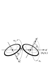
Figure 4: The dinuclear configuration and the coordinates in the rotating molecular frame for an oblate-oblate system. The molecular $z^{\prime}$-axis and the seven degrees of freedom of the system are displayed, where the $\alpha_{1}$- and $\alpha_{2}$-degrees are to be combined into $\theta_{3}=(\alpha_{1}+\alpha_{2})/2$ and the degree of twisting $\alpha=(\alpha_{1}-\alpha_{2})/2$. The figure is taken from Ref. UeNewI. It is the same as published in Refs. Ue94 and UeSuppl.

Internal wave functions for the $R$-matrix calculations are, of course, those of dinuclear molecular model, the characteristic features of which are briefly reminded here, since they are given in detail in the paper I.[3]

Interaction between two nuclei is described with internal collective variables, i.e., the orientations of the poles of the constituent nuclei in the rotating molecular frame. Assuming a constant deformation and the axial symmetry of the constituent nuclei, we are dealing with seven degrees of freedom,

$$(q_{i})=(\theta_{1},\theta_{2},\theta_{3},R,\alpha,\beta_{1},\beta_{2}),$$ (31)

as illustrated in Fig. 4, where $(R,\theta_{2},\theta_{1})$ is the relative vector of the two ${}^{28}\rm Si$. As internal degrees of freedom, the orientations of the symmetry axes of the two ${}^{28}\rm Si$ are described with the Euler angles $(\alpha_{i},\beta_{i})$ which refer to the molecular axes. $\alpha_{1}$ and $\alpha_{2}$ are combined into $\theta_{3}=(\alpha_{1}+\alpha_{2})/2$ and $\alpha=(\alpha_{1}-\alpha_{2})/2$. All those orientation dependences of the interaction are described by a folding-model potential.

It is found that at high spins the dinuclear system with oblate-deformed constituent nuclei has the equilibrium in an equator-equator touching configuration with the parallel principal axes, and that the relative distance between the two ${}^{28}\rm Si$ nuclei is $7-8$fm indicating a nuclear compound system with hyperdeformation. The barrier position (or saddle point) is $9-10$fm, greatly outside from that of the usual optical potential. Molecular ground state configurations are well bound by the barrier up to $J=40$. This theoretical maximum spin is in accord with the bumps observed in the grazing angular momenta.

Since the interaction potential does not couple the states of different $K$-values, at first, we assume the eigenstates of the system to be the rotation-vibration type with a good $K$-quantum number,

$$\Psi_{\lambda}\sim D_{MK}^{J}(\theta_{i})\chi_{K}(R,\alpha,\beta_{1},\beta_{2}),$$ (32)

then the problem to be solved is of internal motions associated with the variables $(R,\alpha,\beta_{1},\beta_{2})$. Couplings among various molecular configurations are taken into account by the method of normal mode around the equilibrium configuration, which gives rise to the molecular modes of excitation. We expand the effective potential at the energy minimum point (the equilibrium relative distance $R_{\rm e}=7.6$fm, $\alpha=\pi/2$ and $\beta_{1}=\beta_{2}=\pi/2$), and adopt the harmonic approximation to obtain the normal modes; the results are as follows. The radial motion has no coupling with the other angle variables, and it is an independent mode in itself. The motions associated with the $\beta$-degrees are well confined to be vibrational ones, which are classified into new modes, butterfly: $\beta_{+}=(\Delta\beta_{1}+\Delta\beta_{2})/\sqrt{2}$ and anti-butterfly: $\beta_{-}=(\Delta\beta_{1}-\Delta\beta_{2})/\sqrt{2}$ around $\alpha=\pi/2$, respectively. As for the $\alpha$-degree, the confinement in the present folding potential appears to be unexpectedly weak, and hence the motion is close to a free rotation, which we call twisting rotational mode. Thus we write the internal wave functions as

$$\chi_{K}(R,\alpha,\beta_{1},\beta_{2})=f_{n}(R)\phi_{K}(\alpha)\varphi_{n_{+}}^{+}(\beta_{+},\alpha)\varphi_{n_{-}}^{-}(\beta_{-},\alpha),$$ (33)

where $\varphi_{n_{+}}^{+}(\beta_{+},\alpha)$ and $\varphi_{n_{-}}^{-}(\beta_{-},\alpha)$ denote the functions describing the $\beta_{+}$ and $\beta_{-}$ modes, respectively. $\alpha$’s in $\varphi_{n_{+}}^{+}(\beta_{+},\alpha)$ and $\varphi_{n_{-}}^{-}(\beta_{-},\alpha)$ are due to the strengths of the confinements in the $\beta_{\pm}$-motions, which vary together with the $\alpha$-motion.

The eigenenergy of the system is given as

$$E^{J}(n,n_{+},n_{-},K,(\nu,\pi_{\alpha})) = E_{0}(R_{\rm e})+{\hbar^{2}\over 2}\bigg{[}{J(J+1)-K^{2}-1\over\mu R_{\rm e}^{2}}+{K^{2}-2\over 2I}\bigg{]}$$ (34)

$$+\Big{(}n+{1\over 2}\Big{)}\hbar\omega_{R}$$

$$+\big{(}n_{+}+n_{-}+1\big{)}\hbar\omega_{0}+E_{\nu}^{\alpha}(\pi_{\alpha}),$$

where the energy is specified by the quantum numbers $(n,n_{+},n_{-},K,(\nu,\pi_{\alpha}))$, with $\nu$ as a dominant frequency of the $\alpha$-motion and with the parity $\pi_{\alpha}$ about the reflection with respect to $\alpha=\pi/2$. The first and second terms on the r.h.s. of Eq. (34) are constant energies that are given by the interaction potential and the centrifugal energy at the equilibrium, respectively, where $I$ denotes the moment of inertia of the constituent nuclei, ${}^{28}\rm Si$, the value of which is estimated from the excitation energy of the $2^{+}_{1}$ state. The term $(n_{+}+n_{-}+1)\hbar\omega_{0}$ gives vibrational energies for the $\beta$-motions without the $\alpha$-dependence, and finally $E_{\nu}^{\alpha}(\pi_{\alpha})$ is the energy for the $\alpha$-motion including the $\alpha$-dependent contribution to the energy of the $\beta$-motions. The values of the vibrational energy quanta for the butterfly and the anti-butterfly modes are both about $4$MeV, but the excitation energies of those modes appear twice, $8$MeV, since states of $K=even$ with one vibrational quantum are not allowed due to the boson symmetry. The excitation energy is close to that of the radial excitation. Although the excited state of the radial mode is not bound in the present calculations, the possibility of the radial-mode resonance is not completely excluded, because it is likely that the interaction between two ${}^{28}\rm Si$ would be more attractive than the present folding potential with the frozen density approximation. It is noted that the $\alpha$-dependence in $\varphi_{n_{\pm}}^{\pm}(\beta_{\pm},\alpha)$ is rather tedious in calculations of the partial widths in the next section. Hence we dropped the $\alpha$-dependence in them, i.e., to be $\varphi_{n_{\pm}}(\beta_{\pm})$ with the average value $4$MeV of $\hbar\omega_{\beta}$, which means that the eigenenergies of the butterfly and anti-butterfly modes are taken to be degenerate. However the properties of those modes are essentially retained with no problem. Of course, for exact calculations, we need total wave functions with the parity and boson symmetries, which are described in Appendix B of the paper I,[3] some examples of the wave functions of the normal modes being also given there in Appendix C.

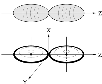
Figure 5: Equilibrium configurations of two di-nuclear systems.   The upper portion is for ${}^{24}\rm Mg-^{24}Mg$   and   the lower one for ${}^{28}\rm Si-^{28}Si$. The figure is taken from Ref. UeNewI.

Wobbling motion ($K$-mixed states)

One of the characteristic features of the spectrum obtained theoretically is a series of low-energy $K$-rotational excitation due to axial asymmetry around molecular z-axis, which is in contrast with the ${}^{24}\rm Mg+{}^{24}Mg$ case.[11, 12] One can understand the reason immediately from Fig. 5, where the upper configuration(${}^{24}\rm Mg+{}^{24}Mg$) has axial symmetry as a total system, but the lower one for ${}^{28}\rm{Si}+{}^{28}\rm{Si}$ has axial asymmetry.

A triaxial system preferentially rotates around the axis with the largest moment of inertia. By the definition of the axes in the lower panel of Fig. 5, we have the moments of inertia as $I_{X}>I_{Y}>>I_{Z}$, due to the nuclear shape. Thus the system, which is seen as two pancake-like objects (${}^{28}\rm Si$’s) touching side-by-side, rotates around $X$-axis normal to the reaction plane. Such a motion is called wobbling, and $K$ is not a good quantum number. Namely, we expect that the eigenstates are $K$-mixed.

Figure 6: Energy spectra of the ${}^{28}\rm Si+{}^{28}Si$ system for $J=38$. (a) Molecular normal modes without $K$-mixing. (b) After $K$-mixing, with indications of the modes under the levels. The figure is taken from Ref. UeNewI.

Regarding the ${}^{28}\rm{Si}+{}^{28}\rm{Si}$ system as a triaxial rotator, as it is usual for polyatomic molecules, we diagonalize the hamiltonian with an inertia tensor of the axial asymmetry, which gives rise to mixings of $K$-projections of the total spin $J$.[31] The resultant motion should be called as ”wobbling mode”.[16] The energy spectrum is displayed in Fig. 6(b), compared with the spectrum without $K$-mixing in Fig. 6(a). Now the states of low lying $K$-series are not the eigenstates by themselves, but are recomposed into new states. It is much interesting that we again obtain several states including the $K=0$ component as a result of $K$-mixing, which should show up themselves in the scattering. Those states are closely located in energy and so in good agreement with several fine peaks observed in the experiment.

As an analytical prescription, in the high spin limit ($K/J\sim 0$), the solution is a gaussian, or a gaussian multiplied by an Hermite polynomial,

$$F_{n}(K)=H_{n}\left({K\over b}\right)\exp\biggl{[}-{1\over 2}\biggl{(}{K\over b}\biggr{)}^{2}\biggr{]}.$$ (35)

The width parameter $b$ is given by

$$b=(2J^{2}{I_{K}/\Delta})^{1/4},$$ (36)

which depends on the ratio between the non-axiality (the difference between $I_{X}$ and $I_{Y}$) and $I_{Z}$ as

$${1\over\Delta}={1\over 2}\bigg{(}{1\over I_{Y}}-{1\over I_{X}}\bigg{)},\qquad{1\over I_{K}}={1\over I_{Z}}-{1\over 2}\bigg{(}{1\over I_{Y}}+{1\over I_{X}}\bigg{)}.$$ (37)

To calculate angular correlations we use those analytic forms in Eq. (35), which is simple and intuitive way to understand the extent of $K$-mixing. Of course we can utilize numerical values obtained in the diagonalization procedure, but the values are almost the same as those given by the analytic form. For the lowest state $F_{0}(K)$ of Eq. (35), we have the wave function for the wobbling ground state as

$$\Psi^{JM}_{\lambda}\sim\sum_{K}\exp(-K^{2}/2b^{2})D_{MK}^{J}(\theta_{i})\chi_{K}(R,\alpha,\beta_{1},\beta_{2}),$$ (38)

where it should be emphasized that, in general, $\chi_{K}$ can be any molecular mode of triaxial deformations, such as the ground-state configuration (parallel equator-equator one), the butterfly mode and the anti-butterfly mode. Then the spin orientations of two ${}^{28}\rm Si$ nuclei are expected to be in the plane, consistent with $"m=0"$, because the nuclei rotate around the axes perpendicular to their symmetry ones. The magnitude of $b$ estimated by Eq. (36) is $1.85$, for example, for the values of the moments of inertia used in the calculations for the energy spectrum in Fig. 6. This is the largest value expected, because we assumed a static configuration there, in which the zero-point motions of the twisting and butterfly modes are neglected. Thus, a value of $b=1.5$ is adopted for the calculations of the physical quantities in the next section. There, it is also examined to what extent a change of $b$ affects the spin disalignments with the orbital angular momentum.

As for the relation between the molecular model and the asymmetric rotator intuitively introduced, we mention that it is clarified in §4.2 of the paper I [3] by using a simple example of the dinuclear system of ”one deformed nucleus and a spherical nucleus”, and thus we do not repeat here.

3 Results

3.1 Structures and partial decay widths of the resonance states

Table 1: Theoretical estimates for partial widths (in keV) in the elastic, single $2^{+}$ and mutual $2^{+}$ channels of the molecular resonances with spin $J=38$ for the theoretical level energies, which are obtained in §2.3. For the wobbling strength, $b=1.5$ is adopted. In parenthesis, widths are given with the assumption of the resonance energy $55.8$MeV.

Molecular states	Energy	$\Gamma_{el}$	$\Gamma_{2^{+}}$	$\Gamma_{(2^{+},2^{+})}$
molecular ground state	51.5MeV	2.1	1.2	0.16
		(19)	(13)	(2.2)
twisting	54.4MeV	0.36	0.24	6.2
		(0.69)	(0.46)	(13)
butterfly	58.9MeV	28	1.5	21
		(8.3)	(0.43)	(5.0)
anti-butterfly	60.3MeV	40	1.5	69
		(8.3)	(0.25)	(15)

In order to analyze structures of the resonance states by the molecular model, we have estimated their partial widths. In Table I, the partial widths of the molecular normal modes with spin $J=38$ are given, up to the mutual $2^{+}$ channel. The results for the $4^{+}$ channels are not shown, since the experimental angular distributions of those channels do not exhibit resonance behaviors.[10, 17] Magnitudes of the widths are calculated with the theoretical level energies, and are obtained to be in the range of several keV to several tens keV, which is consistent with experiment. For comparison, the magnitudes of the widths are also calculated with the assumption that the energy of each state is shifted to the observed resonance energy of $55.8$MeV, and are given in parenthesis. Among the elastic and inelastic channels, characteristic features are seen for each normal mode. As for the molecular ground state, the elastic width is larger than those in the excited channels, which is inconsistent with the experimental characteristics of the narrow resonances. Those weak excitations of the theoretical prediction are inferred to be due to the weak confinement in the $\alpha$-degree of freedom, which permits almost free rotation for the solution with the folding potential. In the butterfly and twisting modes, the mutual $2^{+}$ channel shows strong excitation, but the single $2^{+}$ excitation is very weak, and thus the characteristics are inconsistent with experiment. Therefore neither of the normal modes is completely consistent with the characteristics of the enhanced excitations seen at $E_{\rm cm}=55.8$MeV.

It is, however, meaningful to investigate with a stronger confinement in the $\alpha$-degree of freedom for the molecular ground state, because, in the touching configuration, the confinement possibly increases due to induced deformations of the constituent nuclei. So we investigate the cases with stronger confinements for the $\alpha$-degree with the harmonic oscillator, by using $\hbar\omega_{\alpha}$ as a parameter. This means that we introduce a stronger confinement of the gaussian distribution around the equilibrium, instead of the internal-rotation-like motions, although how much the strength of the confinement should be increased cannot be predicted by the folding model within the frozen density approximation, but is to be quantitatively investigated with the polarization effects or by dynamical treatments of deformations of the constituent ions. The polarization effects of the ions expected to appear will be discussed later in §4.3.

Table 2: Theoretical estimates for partial widths (in keV) in the elastic, single $2^{+}$ and mutual $2^{+}$ channels for the molecular ground state with spin $J=38$ at the experimental resonance energy $E_{\rm cm}=55.8$MeV. Rather confined configurations for the molecular ground state are inspected for (case A: $\hbar\omega_{\alpha}=2$MeV, $\hbar\omega_{\beta}=4$MeV), (case B: $\hbar\omega_{\alpha}=\hbar\omega_{\beta}=4$MeV) and (case C: $\hbar\omega_{\alpha}=\hbar\omega_{\beta}=12$MeV). For the wobbling strength, $b=1.5$ is adopted.

States	$\Gamma_{el}$	$\Gamma_{2^{+}}$	$\Gamma_{(2^{+},2^{+})}$
molecular ground state A	17	12	2.9
molecular ground state B	12	9.2	4.3
molecular ground state C	2.6	3.5	3.0

In Table II, a couple of configurations with stronger confinements are introduced, and the estimations of the partial widths are given at the energy $55.8$MeV. For the configurations named A, B and C, strengths of the confinements are set to be $\hbar\omega_{\alpha}=2$MeV, $4$MeV and $12$MeV, respectively, where in the last case $\hbar\omega_{\beta}=12$MeV is taken consistently with the large value $\hbar\omega_{\alpha}=12$MeV. As the confinement increases, the magnitude of the partial widths in the elastic channel decreases, while excitations to the single and mutual channels are relatively enhanced. With the configuration C, characteristics of the partial widths are in good agreement with the experimental data.[6] Moreover the value of the elastic partial width $2.6$keV is enough small to reproduce the experimentally suggested value, ”a few keV”.[6] Thus the molecular ground state with a well confined configuration is a candidate for the narrow resonance at $55.8$MeV, which is corroborated by the following analyses on fragment angular distributions and fragment-fragment-$\gamma$ angular correlations.

3.2 Fragment angular distributions for the resonance at $E_{\rm cm}=55.8$MeV

Figure 7: Fragment angular distributions for the elastic and inelastic scattering for ${}^{28}\rm Si+{}^{28}Si$ at $E_{\rm cm}=55.8$MeV. From the bottom those for the elastic, single $2^{+}$ and mutual $2^{+}$ are shown. Solid curves are for theoretical results of the molecular ground state with wobbling motion (configuration C), compared with the experimental data.[17]

In Fig. 7, fragment angular distributions are displayed for the elastic scattering, the single $2^{+}$ and the mutual $2^{+}$ excitations. Theoretical angular distributions with the configuration C of the wobbling ground state are compared with the recent data,[17] where their magnitudes are normalized to the single excitation. For the excitations, constant backgrounds of 40% are assumed, because the background yields of about 50% are seen in the experimental data observed by Betts et al.[6] In the elastic scattering, by the phenomenological use of the potential scattering term as in Eq. (19), calculations are made with strong absorption of lower partial waves than the grazing one to reproduce rapid decrease in the differential cross sections toward $\theta_{\rm cm}=90^{\circ}$.[1, 2] Such a rapid decrease is usually seen in the heavy-ion scattering,[25, 32] and it would be one of necessary conditions for the observation of the quite narrow resonances in the elastic scattering. We see good fits for the oscillations, the period of which is close to $L=38$ Legendre polynomials. Magnitudes of the cross sections are qualitatively in good agreement with the data, although the strengths of the excitations are still slightly weak.

3.3 Angular correlations

Figure 8: $\gamma$-ray intensities for particle-particle-$\gamma$ angular correlations in the mutual $2^{+}$ channel. Experimental data are given by dots, and $\chi^{2}$-fits curves are displayed by dashed lines. The theoretical results obtained with the molecular ground state (configuration C: $\hbar\omega_{\alpha}=\hbar\omega_{\beta}=12$MeV) are shown by solid lines. For the quantization axes in three panels, see text.

In the decay process from the molecular resonance state, ${}^{28}\rm Si$-fragments emit $\gamma$-rays due to the transition from the first excited state to the ground state. In the experiment, particle detectors are set to catch the fragments in the direction perpendicular to the incident beam, and the coincident $\gamma$ rays are detected by the $4\pi$ system of Eurogam Phase II.   Figure 8 displays the angular correlation data,[17] i.e., $\gamma$-ray intensity distributions of the $E2$-transition observed in the mutual $2^{+}$ channel and $\chi^{2}$-fits shown by dashed lines. Three different quantization axes are taken in panels (a)$-$(c), respectively: (a) beam direction, (b) $z$-axis normal to the scattering plane, and (c) $z$-axis perpendicular to those of (a) and (b). Since ${}^{28}\rm Si$ fragments are detected in the angular range of $\theta_{\rm cm}=90^{\circ}\pm 7^{\circ}$ in the reaction plane, the $z$-axis of (c) corresponds approximately to final fragment directions.

Theoretical results for the molecular ground state (configuration C of a strong confinement) are displayed by solid lines. In panel (b), we see a typical ”m=0” pattern, which means that the spin directions are in the reaction plane. A weak ”m=0” pattern is seen also in panel (a), while in panel (c), a slight swelling around the center suggests weak ”m=2”.

Table 3: The experimental and theoretical probabilities $P_{m}$ in the magnetic substates $m$, for the mutual $2^{+}$ channel of the resonance state with spin $J=38$ at $E_{\rm cm}=55.8$MeV. The experimental values of $P_{m}$ are obtained by $\chi^{2}$-fits of the data.[17] Theoretical results are given for the molecular ground state, where the first line in (a) shows those for the weak confinement (solution with the folding potential), while the second line in (a) does those for the strong confinement (configuration C: $\hbar\omega_{\beta}=\hbar\omega_{\alpha}=12$MeV), and in (b) and (c) as well. For the wobbling strength, $b=1.5$ is adopted.

Quantization	$P_{m=0}$		$P_{m=\pm 1}$		$P_{m=\pm 2}$
axis	exp.	theor.	exp.	theor.	exp.	theor.
(a)	${0.30\pm 0.08}$	${0.51}$	${0.16\pm 0.04}$	${0.07}$	${0.18\pm 0.05}$	${0.17}$
		${0.20}$		${0.06}$		${0.34}$
(b)	${0.46\pm 0.05}$	${0.70}$	${0}$	${0.01}$	${0.27\pm 0.02}$	${0.14}$
		${0.54}$		${0.18}$		${0.05}$
(c)	${0.14\pm 0.05}$	${0.05}$	${0.17\pm 0.03}$	${0.08}$	${0.26\pm 0.04}$	${0.40}$
		${0.14}$		${0.17}$		${0.26}$

Figure 9: $\gamma$-ray intensities for particle-particle-$\gamma$ angular correlations in the mutual $2^{+}$ channel. Experimental data are given by dots. Dashed lines show theoretical results of the twisting rotational mode, with solid lines for the molecular ground state for comparison. For the quantization axes in three panels, see text.

Figure 10: $\gamma$-ray intensities for particle-particle-$\gamma$ angular correlations in the mutual $2^{+}$ channel. Experimental data are given by dots. Dashed lines show the theoretical results of the butterfly state with $K$-mixing, with solid lines for the molecular ground state for comparison. For the quantization axes in three panels, see text.

Probabilities $P_{m}$ in each magnetic substate $m$ are listed in Table III. Theoretical results of the molecular ground state are given and compared with the experimental data,[17] where the upper line in each axis case is for a weak confinement case (solution with the folding potential), while the second line is for a strong confinement (configuration C), respectively. In (b), theoretical results reproduce dominant ”m=0” characteristics, for both configurations of the weak and strong confinements. Thus, the ”m=0” characteristics of the angular correlations do not depend essentially upon the strength of the confinement in the $\alpha$-degree of freedom. $|m|=2$ contributions in (b) appear slightly weak, compared with the experimental data, but this suggests $|m|=2$ contribution from the background.[10] As for the values of $P_{m}$ in (a) and (c), they are also in good agreements with the data, although they vary depending on the strengths of the confinements.

To clarify properties of the normal mode excitations in the angular correlations, we make analyses for the twisting and butterfly modes, which are of interest as they exhibit strong excitation to the mutual $2^{+}$ channel. In Fig. 9, the angular correlations of the twisting mode are displayed with dashed lines, and comparison with the molecular ground state (solid lines) is given. Apparently, the twisting excitation does not fit the experimental data. The characteristic feature of twisting is ”m=2” dominance in (a), which is due to the excited rotational motion in the $\alpha$-degree of freedom.

In Fig. 10, results are displayed with dashed lines for the butterfly mode with $K$-mixing. The results for the anti-butterfly mode appear to be quite similar to those of the butterfly mode (not shown here). Again, solid lines are those for the molecular ground state for comparison. The butterfly excitations show their own characteristics with dominant ”m=1” patterns in the panels (a) and (b). In addition, they exhibit ”m=2” dominance in (c), due to the butterfly vibrational motions. Thus all those theoretical results for the normal mode excitations are much different from the data at the resonance energy $55.8$MeV, and moreover they show quite distinguishing characteristics.

Note that the configurations of the molecular ground state in Figs. 8, 9 and Fig. 10 are not completely the same due to changes of the confinement parameter value, and one can confirm differences between the results with different strengths of confinements in the $\alpha$-degree of freedom. In Fig. 9, the most weak confinement is taken from the solution with the folding potential, and in Fig. 10 a slightly stronger confinement is taken (the configuration A: $\hbar\omega_{\alpha}=2$MeV, $\hbar\omega_{\beta}=4$MeV). All those configurations give ”m=0” characteristics, and the differences between them are not significant.

Figure 11: $\gamma$-ray intensities for particle-particle-$\gamma$ angular correlations in the single $2^{+}$ channel. Experimental data are given by dots, and $\chi^{2}$-fits by dashed lines, respectively. Solid lines show the theoretical results obtained with the molecular ground state with wobbling motion (configuration C). For the quantization axes in three panels, see text.

The magnitude of wobbling ($K$-mixing) is taken to be $b=1.5$, which is consistent with the asymmetry of the ${}^{28}\rm{Si}+{}^{28}\rm{Si}$ molecular ground-state configuration, as it is estimated to be $b=1.85$ in the limit of the strong confinement (without quantum fluctuations). The parameter for the $K$-mixing is examined in the range of $b=1.2-2.0$ with the configuration C. The value of $P_{m=0}$ in (b) varies from 0.4 to 0.8 with the increasing value of $b$, but for the configurations with the strong confinements the resultant curves are seen to be essentially the same in those values of $b$.

Next we move to the single $2^{+}$ excitation. In Fig. 11, the experimental data are displayed, together with $\chi^{2}$-fits given by dashed lines.[10] The theoretical results for the molecular ground state (configuration C of a strong confinement) are shown by solid lines. Surprisingly, the experimental data are seen to be quite similar to those of the mutual $2^{+}$ channel, and again ”m=0” characteristics in (b) are firstly of interest. The present model reproduces the characteristics well. Theoretical results exhibit totally good fits with the data, although the fits in panel (a) are not very good, with rather large $m=0$ contribution. However, contributions of the background from aligned configurations are expected to provide $|m|=1$ components in (a) and (c), and thus those slight deviations of the fits are not serious.

4 Discussion

4.1 Structure of the ${}^{28}Si-{}^{28}Si$ molecule

In the paper I,[3] interaction between two ${}^{28}\rm Si$ nuclei is described with the internal collective variables, i.e., with the orientations of the poles of the constituent nuclei in the rotating molecular frame. For the dinuclear system with oblate-deformed constituent nuclei, an equator-equator touching configuration is found to be the equilibrium at high spins where the principal axes of the constituent nuclei are parallel. The relative distance between the two ${}^{28}\rm Si$ nuclei is $7-8$fm indicating a nuclear compound system with hyperdeformation. The barrier position is $9-10$fm, greatly outside from that of usual optical potentials. Molecular ground state configurations are well stable by the barrier up to $J=40$. This theoretical maximum spin is in accord with the bumps observed in grazing angular momenta.

Couplings among various molecular configurations are taken into account by the method of normal mode around the equilibrium configuration, which gives rise to the molecular modes of excitation, such as the radial vibration, the butterfly motion, the anti-butterfly motion and so on. The twisting mode ($\nu=4$) appears to be the lowest excitation, but the energy may be higher than the present results due to a stronger confinement as physically expected, which will be discussed later in §4.3.

Since the equilibrium configuration has a triaxial shape, we extend our molecular model so as to include couplings between states with different $K$-quantum numbers. In practice, we use the asymmetric rotator as an intuitive model, which preferentially rotates around the axis of the largest moment of inertia, accompanied with $K$-mixing, and thus gives rise to the wobbling motion.

4.2 On the spin disalignments

An important physical quantity which probes the structure of the resonance states is spin alignments of the outgoing particles. The recent experiment on the ${}^{28}\rm Si+{}^{28}Si$ resonance at $E_{\rm cm}=55.8$MeV suggests $L=J=38$ dominance in the inelastic scattering both to the single and mutual $2^{+}$ excitations. Measured particle-particle-$\gamma$ correlations show ”m=0” dominance in $\gamma$-rays. All these suggest that the spin vectors are in the reaction plane.[10, 17]

The analyses are made for the molecular model wave functions. In the state with the lowest energy of a given angular momentum $J$, due to the triaxial configuration, the whole system rotates about the axis normal to the reaction plane defined by the two pancake-like nuclei. The spins of the ²⁸Si fragments are thus in this plane, since no rotation can occur about the symmetry axes of the ²⁸Si nuclei. Such a property is in agreement with the lack of strong alignments observed in the fragment angular distributions. Actually, ”m=0” dominances in the angular correlations are well reproduced for the single and mutual $2^{+}$ excitations.

Characteristic features of the angular correlations in the normal mode excitations are found to be dominant ”m=2” patterns, i.e., for the twisting rotational mode ”m=2” appears in (a)-axis, and for the butterfly mode it appears in (c)-axis, respectively. This means that spin vectors are parallel to the beam direction in the twisting mode, while parallel to the fragment direction in the butterfly mode. (The reason for those orientations of the spin vectors is explained later.) One may expect that the twisting mode and/or the butterfly mode are favorable for the ”m=0” characteristic, because spin orientations are in the reaction plane. However, more precisely, ”m=0” means symmetric around the normal axis, which is satisfied by neither of excited states such as twisting nor butterfly with a well-defined direction of the spin in the reaction plane. The existence of dominant $m=2$ substates, together with ”m=1” patterns in the other panels, are clear characteristics of the normal modes. Thus, it is possible to distinguish among the molecular ground state, the twisting excitation and the butterfly excitations, respectively.

Finally, we discuss the observed spin directions in space, with respect to the orientation of the molecular $z^{\prime}$-axis at the time of decay, which is related to the positions of the particle detectors in the angular correlation measurements. For example, in the twisting mode, the ${}^{28}\rm{Si}$ nuclei rotate around the molecular $z^{\prime}$-axis, and so the spin vectors are parallel to it. Since the fragments ${}^{28}\rm Si$ are detected approximately at $\theta_{\rm cm}=90^{\circ}$ (the (c)-axis direction), the molecular $z^{\prime}$-axis and the spin vectors are expected to be approximately parallel to (c)-axis. However our theoretical prediction does not exhibit the ”m=2” pattern in (c). Unexpectedly, it appears in (a)-axis (the beam axis), as is displayed in Fig. 9 with dashed lines, which gives rise to a puzzle. This is an interesting aspect of extremely-high spin resonances. Due to the high-speed rotational motion, the final velocity vectors of the fragments are considered to be almost perpendicular to the relative vector of the fragments in the decay process, like raindrop motions splashed from a rapidly rotating umbrella. In order to examine the motions of the ${}^{28}\rm{Si}$ nuclei after the decay, we have analyzed classical orbits and obtained results that for $J=38$ the relative vector turns round about $70^{\circ}$ from the initial angle. As a confirmation, we calculated angular correlations with a relatively lower angular momentum $J=8$. The results show the ”m=2” dominance in (c)-axis, as expected by the above explanation.

4.3 Strengths of confinements

With respect to the very narrow resonances observed as correlating among the elastic and inelastic scattering, partial decay widths are investigated. In the butterfly and the twisting modes, the decay probability amplitudes concentrate to the elastic and mutual $2^{+}$ channels. This is a characteristic feature of the normal mode excitations, which is due to the symmetric motions of the two ${}^{28}\rm Si$ nuclei. Such characteristics are, however, not seen in the data at $E_{\rm cm}=55.8$MeV. The molecular ground state or the radially-excited state obtained by using the folding potential shows rather large elastic widths and weak excitations to the inelastic channels. Hence, the properties of the partial widths observed at $E_{\rm cm}=55.8$MeV have not been well reproduced for all those states.

It is worth to have a close look at the results with the folding-model potential. The molecular ground state configuration obtained by using the folding potential with the frozen density approximation, exhibits very weak confinement in the twisting degree of freedom, which results in an almost-free rotation. Intuitively, the extreme weak or shallow potential in the twisting motion appears unphysical, because the two ${}^{28}\rm Si$ nuclei are touching with each other. That is, the folding model with the frozen density is not well adequate. Actually, the modification of the confinement in terms of larger values of $\hbar\omega$ for the twisting and consistently for the butterfly motions shows that the partial decay width in the elastic channel greatly reduces, while those in the inelastic channels relatively increase. As a result, the magnitudes of the partial widths become to be consistent with the experimental characteristics, which finally gives good agreements with the experimental data for the fragment angular distributions. Thus, the analyses suggest a substantial change of the deformation of the constituent nuclei and/or formation of a neck between them, which gives rise to a stronger confinement than that obtained by the folding model. This is exactly consistent with the existence of the stable triaxial configuration. In addition, experimental observations suggesting the stronger confinement are known in the ${}^{24}\rm Mg+{}^{24}Mg$ system. Only 30% of the resonance flux appears in the binary decay channels of ${}^{24}\rm Mg+{}^{24}Mg$.[9] A search for the remaining flux to the fusion-evaporation channels has been recently made.[33] Those observations suggest that two incident nuclei interact with each other strongly with their density overlapping and induced deformations. Their effects would be described effectively by a stronger confinement. A mechanism for the strong confinement is intriguing and yet to be clarified theoretically.

4.4 Observation conditions

Finally, observation conditions of resonances in heavy-ion reactions should be discussed. In experimental excitation functions of the ${}^{28}\rm Si+{}^{28}Si$ system which are angle-averaged around $\theta_{\rm cm}=90^{\circ}$, background yields of the elastic scattering and of the single and mutual $2^{+}$ excitations decrease rapidly as the bombarding energy increases toward the resonance region.[6, 7] The same is the case in the ${}^{24}\rm Mg+{}^{24}Mg$ system.[8]Such low background yields are one of the conditions to clearly observe resonances. Especially in the elastic scatterings, strong damping of non-resonant amplitudes is a necessary condition, because the resonance yields themselves are very small. Over those background yields, many prominent peaks would be observed with relatively large yields in the channels concerned, which theoretically have to be well described by the resonance terms, such as by the $R$-matrix theory. Strong absorption by the smooth cutoff model has worked as a successful description for the elastic background scattering in the angular distributions, as well as appropriate optical model analyses. Actually, in the ${}^{28}\rm Si+{}^{28}Si$ system, it is shown that the effects of the strong absorption do not necessarily work to eliminate resonance structures, but show up very narrow and prominent structures over the very low background. This is quite different from the conditions of the resonances observed in lighter systems such as ${}^{12}\rm C+{}^{12}C$ and ${}^{16}\rm O+{}^{16}O$, where weak absorption plays a crucial role.[15]

5 Conclusions

Resonances in the ${}^{28}\rm Si+{}^{28}Si$ system have been studied by means of the molecular model, in which the interacting dinuclear system is described by the molecular rotation and the internal collective variables for the orientations of the poles of the constituent nuclei. The molecular model predicts rotational spectra with a variety of intrinsic molecular states, such as the butterfly, twisting and etc. In order to explore which one of the various molecular modes agrees with the experimental data on the resonance at $E_{\rm cm}=55.8$MeV, we have performed comprehensive analyses on available physical quantities, i.e., on partial widths, fragment angular distributions and fragment-fragment-$\gamma$ angular correlations.

Among the various modes, the molecular ground state with $J=38$ is successfully selected to be a candidate for the resonance observed at $E_{\rm cm}=55.8$ MeV. We have found that for the resonance state, a nuclear molecule ${}^{28}\rm Si-{}^{28}Si$ of triaxial shape wobblingly rotates with a very high spin. The present results are the first discovery of the modes with $K$-mixing in heavy-ion resonance states, though the tilting or wobbling mode was once discussed in deep inelastic scattering processes.[34]

In the partial decay widths, each normal mode shows an interesting feature, i.e., resonance amplitudes appear to be enhanced in each relevant characteristic channels. Moreover, the butterfly modes show fragment spins in the fragment direction (”m=2”), while the twisting mode does in the beam direction. Since each normal mode shows its own distinct characteristics of the angular correlations, it is possible to identify each excitation of the modes. Thus, angular correlation measurements are a powerful tool for the study of nuclear structures of heavy-ion resonances. Systematic measurements are desired, not only on the resonance at $E_{\rm cm}=55.8$MeV. For example, the same kind of measurements on the other nearby resonances of ${}^{28}\rm Si+{}^{28}Si$ is strongly called for.

Appendix A Relation between Molecular Wave Functions and Channel Wave Functions for Calculating Decay Properties

The total system consists of two deformed nuclei, for which we have assumed the axial symmetry and constant deformations. We have seven degrees of freedom illustrated in Fig. 12(a) except for the center of mass motion for the whole system, that is, the relative vector $\hbox{\mbf R}=(R,\theta_{2},\theta_{1})$ and the orientations of the deformations of the interacting nuclei described with Euler angles $({\tilde{\alpha}}_{1},{\tilde{\beta}}_{1})$ and $({\tilde{\alpha}}_{2},{\tilde{\beta}}_{2})$. Thus with those variables, generalized channel wave functions of $\{(I_{1}I_{2})Il,JM\}$ scheme are defined as usual in the $R$-matrix theory. Specifying the spins $I_{1}$ and $I_{2}$ for the two constituent nuclei, a function with channel spin $I$ is given by

$$\psi_{(I_{1}I_{2})IM_{I}}=\sum_{M_{1}M_{2}}(I_{1}I_{2}M_{1}M_{2}|IM_{I})\chi_{I_{1}M_{1}}({\tilde{\alpha}_{1}},{\tilde{\beta}_{1}})\chi_{I_{2}M_{2}}({\tilde{\alpha}_{2}},{\tilde{\beta}_{2}}),$$ (39)

where $\chi_{I_{i}M_{i}}({\tilde{\alpha}_{i}},{\tilde{\beta}_{i}})$ denote internal wave functions for the constituent nuclei ${}^{28}\rm Si$. The generalized channel wave function is given with the orbital angular momentum $l$ for the relative motion,

$$\hbox{\calg Y}_{(I_{1}I_{2})Il,JM}=\sum_{M_{I},m}(IlM_{I}m|JM)\hbox{\calg S}_{12}\big{[}\psi_{(I_{1}I_{2})IM_{I}}Y_{lm}(\theta_{2},\theta_{1})\big{]},$$ (40)

where $\hbox{\calg S}_{12}=(1+\hbox{\calg P}_{12})/{\sqrt{2(1+\delta_{I_{1}I_{2}})}}$ denotes the symmetry operator between two ${}^{28}\rm Si$ nuclei. The internal wave functions in Eq. (39) are assumed to be a rotational type, such as,

$$\chi_{I_{i}M_{i}}({\tilde{\alpha}_{i}},{\tilde{\beta}_{i}})=\sqrt{2I_{i}+1\over 8\pi^{2}}D^{I_{i}}_{M_{i}0}({\tilde{\alpha}_{i}},{\tilde{\beta}_{i}},{\tilde{\gamma}_{i}}),$$ (41)

where $K_{i}=0$ are given in consistent with the axial symmetry of the constituent nuclei assumed, and hence ${\tilde{\gamma}_{i}}$ are spurious and do not appear in the l.h.s of Eq. (41).

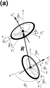
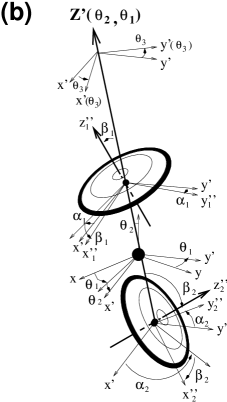
Figure 12: The coordinates of an interacting dinuclear system. (a) shows the relative vector $\boldsymbol{R}=(R,\theta_{2},\theta_{1})$ and usual Euler angles $({\tilde{\alpha}}_{i},{\tilde{\beta}}_{i})$ of the $i$-th nucleus referring to the laboratory frame. In (b), the molecular $z^{\prime}$-axis and the seven degrees of freedom of the system are displayed, where the distance $R$ is not indicated explicitly. The third angle $\theta_{3}$ is defined by $\theta_{3}=(\alpha_{1}+\alpha_{2})/2$ to give the whole rotation around the $z^{\prime}$-axis. The figure is taken from Ref. UeNewI.

Next we define variables in the molecular coordinate system for the model wave functions. As is illustrated in Fig. 12(b), we define a rotating molecular axis $z^{\prime}$ of the whole system with the direction of the relative vector R of the two interacting nuclei. In the molecular model, orientations and/or motions of the intrinsic axes of each deformed nucleus are referred to the molecular axes as usual. For describing those orientations, we introduce new Euler angles $(\alpha_{1},\beta_{1},\gamma_{1})$ and $(\alpha_{2},\beta_{2},\gamma_{2})$, relations of which with the Euler rotations $({\tilde{\alpha}_{i}},{\tilde{\beta}_{i}},{\tilde{\gamma}_{i}})$ referred to the laboratory system are given as

$$\Omega_{i}({\tilde{\alpha}}_{i},{\tilde{\beta}}_{i},{\tilde{\gamma}}_{i})=\Omega^{\prime}_{i}(\alpha_{i},\beta_{i},\gamma_{i})\Omega_{M}(\theta_{1},\theta_{2}),\qquad i=1,\,\,2,$$ (42)

where $\Omega_{i}$ and $\Omega^{\prime}_{i}$ denote Euler rotations for the $i$-th constituent nucleus with respective angles, and $\Omega_{M}$ denotes rotations of the molecular axes. On the r.h.s. of Eq. (42) $\Omega^{\prime}_{i}$ denote the successive rotations after $\Omega_{M}$; firstly the axes of the $i$-th constituent nucleus rotate up to the directions of the molecular axes by $\Omega_{M}$, and secondly they rotate referring to the molecular axes by $\Omega^{\prime}_{i}$. Since the second rotations are written as $\Omega^{\prime}_{i}(\alpha_{i},\beta_{i},\gamma_{i})=\Omega_{M}(\theta_{1},\theta_{2})\Omega_{i}(\alpha_{i},\beta_{i},\gamma_{i})\Omega^{-1}_{M}(\theta_{1},\theta_{2})$ with rotations $\Omega_{i}(\alpha_{i},\beta_{i},\gamma_{i})$ referring to the laboratory system, we obtain

$$\Omega_{i}({\tilde{\alpha}}_{i},{\tilde{\beta}}_{i},{\tilde{\gamma}}_{i})=\Omega_{M}(\theta_{1},\theta_{2})\Omega_{i}(\alpha_{i},\beta_{i},\gamma_{i}),$$ (43)

and accordingly we are able to define the new Euler angles $(\alpha_{i},\beta_{i},\gamma_{i})$ by the relations

$$\Omega_{i}(\alpha_{i},\beta_{i},\gamma_{i})=\Omega^{-1}_{M}(\theta_{1},\theta_{2})\Omega_{i}({\tilde{\alpha}}_{i},{\tilde{\beta}}_{i},{\tilde{\gamma}}_{i}).$$ (44)

Note that $\gamma_{i}$ are spurious as well as ${\tilde{\gamma}}_{i}$, and so we neglect them in the following descriptions.

The molecular $x^{\prime}$-axis would be determined with the two constituent nuclear configurations around the $z^{\prime}$-axis which are specified by $\alpha_{i}$. Hence they are combined into $\theta_{3}=(\alpha_{1}+\alpha_{2})/2$ and $\alpha=(\alpha_{1}-\alpha_{2})/2$, and then we have molecular coordinates,

$$(q_{i})=(\theta_{1},\theta_{2},\theta_{3},R,\alpha,\beta_{1},\beta_{2}),$$ (45)

where $\theta_{1},\theta_{2}$ and $\theta_{3}$ are the Euler angles of the rotating molecular frame with the other fours being internal variables. The molecular $x^{\prime}$- and $y^{\prime}$-axes defined with $\theta_{3}$ are illustrated as $x^{\prime}(\theta_{3})$ and $y^{\prime}(\theta_{3})$ in Fig. 12(b). With the definition of the molecular $x^{\prime}$-axis with $\theta_{3}$, rotational angles of each constituent nucleus should be redefined so that $\alpha_{1}(\theta_{3})=\alpha_{1}-\theta_{3}=\alpha$ and $\alpha_{2}(\theta_{3})=\alpha_{2}-\theta_{3}=-\alpha$. Here after we write them as $\alpha_{i}$ simply, and correspondingly the relations Eq. (43) are rewritten as

$$\Omega_{i}({\tilde{\alpha}}_{i},{\tilde{\beta}}_{i})=\Omega_{M}(\theta_{1},\theta_{2},\theta_{3})\Omega_{i}(\alpha_{i},\beta_{i}).$$ (46)

Now, by means of relations (46), the internal wave functions of Eq. (41) are written with the molecular coordinates as

$$\chi_{I_{i}M_{i}}({\tilde{\alpha}_{i}},{\tilde{\beta}_{i}})=\sum_{\mu_{i}}D^{I_{i}}_{M_{i}\mu_{i}}(\theta_{1},\theta_{2},\theta_{3})\chi_{I_{i}\mu_{i}}(\alpha_{i},\beta_{i}).$$ (47)

We substitute Eq. (47) into Eqs. (39) and (40), and use the following relations,

$$\sum_{M_{1}M_{2}}(I_{1}I_{2}M_{1}M_{2}|IM_{I})D^{I_{1}}_{M_{1}\mu_{1}}(\theta_{i})D^{I_{2}}_{M_{2}\mu_{2}}(\theta_{i})=(I_{1}I_{2}\mu_{1}\mu_{2}|I\,\mu_{1}+\mu_{2})D^{I}_{M_{I},\,\mu_{1}+\mu_{2}}(\theta_{i}),$$ (48)

$$\sum_{M_{I},m}(IlM_{I}m|JM)D^{I}_{M_{I},\,\mu_{1}+\mu_{2}}(\theta_{i})Y_{lm}(\theta_{2},\theta_{1})=$$

$$(Il\,\mu_{1}+\mu_{2}\,\,0|J\,\,\mu_{1}+\mu_{2}){\sqrt{(2l+1)/4\pi}}\,D^{J}_{M,\,\mu_{1}+\mu_{2}}(\theta_{i}),$$ (49)

where $\theta_{i}$ is the abbreviation for $\theta_{1},\theta_{2},\theta_{3}$. Thus we obtain the generalized channel wave function expressed with the molecular coordinates,

$$\hbox{\calg Y}_{(I_{1}I_{2})Il;JM}=\sum_{K}(IlK0|JK){\sqrt{2l+1\over 4\pi}}\hbox{\calg S}_{12}\big{[}D^{J}_{MK}(\theta_{i})\Phi_{(I_{1}I_{2})IK}(\alpha,\beta_{1},\beta_{2})\big{]},$$ (50)

with

$$\Phi_{(I_{1}I_{2})IK}(\alpha,\beta_{1},\beta_{2}) = \sum_{\mu_{1}\mu_{2}}(I_{1}I_{2}\mu_{1}\mu_{2}|IK)\chi_{I_{1}\mu_{1}}(\alpha,\beta_{1})\chi_{I_{2}\mu_{2}}(-\alpha,\beta_{2})$$ (51)

$$= \sum_{\mu_{1}\mu_{2}}(I_{1}I_{2}\mu_{1}\mu_{2}|IK)\,{\rm e}^{i\nu\alpha}d^{I_{1}}_{\mu_{1}0}(\beta_{1})d^{I_{2}}_{\mu_{2}0}(\beta_{2}),$$

where $\nu\equiv\mu_{1}-\mu_{2}$ denotes twisting quantum number. As the generalized channel wave functions are expanded with the rotational functions for the whole system in a series of $K=\mu_{1}+\mu_{2}$, we are able to easily calculate overlapping integrals between each channel wave function with $\{(I_{1}I_{2})Il,JM\}$ and the model wave functions specified with $\{JMK\}$. Note that in the $R$-matrix formula in §2 and for the generalized channel wave functions given above, normalization integrals are defined as usual, while the definition of the model wave functions $\Psi_{\lambda}$ in Eqs. (32) and (33) is given for the vibrational modes with the volume element $dV=dRd\alpha d\beta_{1}d\beta_{2}$ (see §2.2 of the paper I[3] for details). Hence, for the internal wave functions $\Psi^{JM}_{\lambda}$ in Eq. (8), we use $\Psi_{\lambda}/\sqrt{D}$, where $\Psi_{\lambda}$ denote the model wave functions and $D=\mu^{3/2}R^{2}I_{1}\sin\beta_{1}I_{2}\sin\beta_{2}$, square root of which is the additional phase factor of the molecular model wave functions.

Finally we mention the property of the channel functions described in the molecular coordinate system. Due to the angular momentum coupling $(I_{1}I_{2}\mu_{1}\mu_{2}|IK)$, we have restrictions $\mu_{1}\leq I_{1}$, $\mu_{2}\leq I_{2}$ and $K=\mu_{1}+\mu_{2}\leq I$ for the summations on $K$ and $(\mu_{1},\mu_{2})$ in Eqs. (50) and (51). For the elastic channel, where $I_{1}$ and $I_{2}$ are to be equal to $0$, the values of $\mu_{1}$ and $\mu_{2}$ are zero and so the same as for $K$ and $\nu$. Hence the elastic channel wave function has no real $\alpha$-dependence nor $\beta_{i}$-dependence, and it is described simply by $D^{J}_{M0}(\theta_{1},\theta_{2},\theta_{3})$, i.e., by $Y_{JM}(\theta_{2},\theta_{1})$. Thus, due to the boson symmetry, we have only positive-parity states with $l=J=even$, as usual.

References

- [1] R. R. Betts, Proc. Intern. Conf. on Nuclear Physics with Heavy Ions, Stony Brook, 1983, ed. P. Braun-Munzinger (Harwood academic pub., New York, 1984), p. 347.
- [2] R. R. Betts, Proc. 4th Intern. Conf. on Clustering Aspects of Nuclear Structure and Nuclear Reactions, Chester, 1984, eds. J.S. Lilley and M.A. Nagarajan (D. Reidel, Dordrecht, 1985), p. 133.
- [3] E. Uegaki and Y. Abe, Prog. Theor. Phys. 127 (2012), 831.
- [4] R. R. Betts, S. B. DiCenzo and J. F. Petersen, Phys. Rev. Lett. 43 (1979), 253.
- [5] R. R. Betts, S. B. DiCenzo and J. F. Petersen, Phys. Lett. 100B (1981), 117.
- [6] R. R. Betts, B. B. Back and B. G. Glagola, Phys. Rev. Lett. 47 (1981), 23.
- [7] S. Saini and R. R. Betts, Phys. Rev. C 29 (1984), 1769.
- [8] R. W. Zurmühle et al., Phys. Lett. 129B (1983), 384.
- [9] S. Saini et al., Phys. Lett. B185 (1987), 316.
- [10] C. Beck, R. Nouicer, et al., Phys. Rev. C 63 (2000), 014607.
- [11] E. Uegaki and Y. Abe, Phys. Lett. B 231 (1989), 28.
- [12] E. Uegaki and Y. Abe, Prog. Theor. Phys. 90 (1993), 615.
- [13] E. Uegaki and Y. Abe, Phys. Lett. B 340 (1994), 143.
- [14] E. Uegaki, Prog. Theor. Phys. Suppl. No. 132 (1998), 135.
- [15] Y. Abe, Y. Kondō and T. Matsuse, Prog. Theor. Phys. Suppl. No. 68 (1980), 303, and references therein.
-
[16]
S. W. Ødegård et al.,
Phys. Rev. Lett. 86 (2001), 5866.
Y. R. Shimizu, M. Matsuzaki and K. Matsuyanagi, Phys. Rev. C 72 (2005), 014306. - [17] R. Nouicer, C. Beck, et al., Phys. Rev. C 60 (1999), 041303(R).
- [18] W. Trombik et al., Phys. Lett. 135B (1984), 271.
- [19] D. Konnerth et al., Phys. Rev. Lett. 55 (1985), 588.
- [20] A. Mattis et al., Phys. Lett. B 191 (1987), 328.
- [21] D. Konnerth et al., Proc. Fifth Intern. Conf. on Clustering Aspects in Nuclear and Subnuclear Systems, Kyoto, 1988: J. Phys. Soc. Jpn. 58 (1989), Suppl. p. 325.
- [22] A. H. Wuosmaa et al., Phys. Rev. Lett. 58 (1987), 1312; Phys. Rev. C 41 (1990), 2666.
- [23] P. L. Kapur and R. E. Peierls, Proc. R. Soc. Lond. A 166 (1938), 277.
- [24] A. M. Lain and R. G. Thomas, Rev. Mod. Phys. 30 (1958), 257.
- [25] W. E. Frahn and R. H. Venter, Ann. Phys.(NY) 24 (1963), 243, and references therein.
- [26] J. A. McIntyre, S. D. Baker and K. H. Wang, Phys. Rev. 125 (1962), 584.
- [27] For example, F. Rybicki, T. Tamura and G. R. Satchler, Nucl. Phys. A146 (1970), 659.
- [28] C. Beck, private communications.
- [29] For example, W. Dünnweber, in Proc. Intern. School of Phys. ”Enrico Fermi” Course 87, Nuclear Structure and Heavy-Ion Dynamics, eds. L.G. Moretto and R.A. Ricci (North-Holland, Amsterdam, 1984), p. 389.
- [30] A. Bohr, Nucl. Phys. 10 (1959), 486.
- [31] A. Bohr and B. R. Mottelson, Nuclear Structure vol. II (Benjamin, Massachusetts, 1975), p. 175.
- [32] P. Braun-Munzinger and J. Barrette, Phys. Rep. 87 (1982), 209, and references therein.
- [33] M.-D. Salsac et al., Nucl. Phys. A 801 (2008), 1.
- [34] J. Randrup, Nucl. Phys. A447 (1986), 133. See also L. G. Moretto, G. F. Peaslee and G. J. Wozniak, Nucl. Phys. A502 (1989), 453.