Classical and Quantum Chaos in the Diamond Shaped Billiard

Abstract

We analyse the classical and quantum behaviour of a particle trapped in a diamond shaped billiard. We defined this billiard as a half stadium connected with a triangular billiard. A parameter $\xi$ which gradually change the shape of the billiard from a regular equilateral triangle ($\xi=1$) to a diamond ($\xi=0$) was used to control the transition between the regular and chaotic regimes. The classical behaviour is regular when the control parameter $\xi$ is one; in contrast, the system is chaotic when $\xi\neq 1$ even for values of $\xi$ close to one. The entropy grows fast as $\xi$ is decreased from 1 and the Lyapunov exponent remains positive for $\xi<1$. The Finite Difference Method was implemented in order to solve the quantum problem. The energy spectrum and eigenstates were numerically computed for different values of the control parameter. The nearest-neighbour spacing distribution is analysed as a function of $\xi$, finding a Poisson and a Gaussian Orthogonal Ensemble (GOE) distribution for regular and chaotic regimes respectively. Several scars and bouncing ball states are shown with their corresponding classical periodic orbits. Along the document the classical chaos identifiers are computed to show that system is chaotic. On the other hand, the quantum counterpart is in agreement with the Bohigas-Giannoni-Schmit conjecture and exhibits the standard features for chaotic billiard such as the scarring of the wavefunction.

Keywords: quantum chaos, quantum billiards, random matrices, FDM

1 Introduction

A billiard is a system where a particle, with mass $m$, is trapped in a region $\mathfrak{D}$ with perfect reflecting walls. The dynamics of the particle varies depending on the shape of the billiard boundary $\partial\mathfrak{D}$. The cardioid billiard, the Bunimovich billiard (stadium billiard) and non-equilateral triangular billiards are typical examples which exhibit classical chaos. The quantum problem is reduced to solve the Hemholtz equation for the wave function $\psi(\vec{r})$

$$\left(\vec{\nabla}^{2}+\kappa^{2}\right)\psi(\vec{r})=0\hskip 14.22636pt\mathrm{for}\hskip 14.22636pt\vec{r}\in\mathfrak{D}$$ (1)

with the Dirichlet boundary condition $\psi(\vec{r})=0$ if $\vec{r}\in\partial\mathfrak{D}$ where $\kappa=\sqrt{2mE}/\hbar$ is the wave vector and $E$ is the energy. The energy level statistical properties of several Hamiltonian systems may be studied borrowing results from the random matrices theory. For example, it is well known that the energy level spacing distributions of a system is Poissonian if its classical counterpart exhibits a regular motion. This is the case of billiards whose shape is a rectangle (particle in a two dimensional box), an equilateral triangle, a circle or an ellipse. On the other hand, if the classical counterpart has a chaotic motion, then the energy levels follow a Gaussian Orthogonal Ensemble (GOE) distribution [1]. Other non convex and chaotic two dimensional quantum cavities are the Sinai and the annular billiards. They introduce an inner disk of infinite potential into the rectangular and circular billiards respectively.

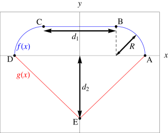
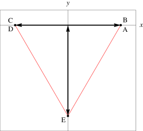
Figure 1: (left) The diamond shaped billiard is defined through the functions $f(x)$ and $g(x)$. In turn, these functions depend on the parameters $R$, $d_{1}$ and $d_{2}$. (right) Triangular billiard.

The system studied in this paper is the diamond shaped billiard (see Figure 1). The upper boundary of the billiard is a half stadium defined by the equation $y=f(x)$ with

$$f(x)=\left\{\begin{array}[]{ll}\sqrt{R^{2}-\left(x+\frac{d_{1}}{2}\right)^{2}}&\mbox{ if $-R-\frac{d_{1}}{2}<x\leq-\frac{d_{1}}{2}$}\\ R&\mbox{ if $|x|\leq\frac{d_{1}}{2}$}\\ \sqrt{R^{2}-\left(x-\frac{d_{1}}{2}\right)^{2}}&\mbox{ if $\frac{d_{1}}{2}<x\leq\frac{d_{1}}{2}+R$}\end{array}\right.$$ (2)

and the lower boundary as $y=g(x)$ with

$$g(x)=\left\{\begin{array}[]{rl}\displaystyle\frac{-d_{2}x}{R+\frac{d_{1}}{2}}-d_{2}&\mbox{ if $-R-\frac{d_{1}}{2}<x<0$}\\ \displaystyle\frac{d_{2}x}{R+\frac{d_{1}}{2}}-d_{2}&\mbox{ if $0<x<R+\frac{d_{1}}{2}$}\end{array}\right.$$ (3)

The parameters which define the billiard depend on the control parameter $\xi$ according to: $R(\xi)=R_{o}\left(1-\xi\right)$, $d_{1}(\xi)=\left(\frac{5}{2}+\xi\right)R_{o}$ and $d_{2}(\xi)=\sqrt{\frac{3}{4}}d_{1}(\xi)$. The value of $R_{o}$ has been taken as one and the non-dimensional parameter $\xi$ varies in the interval $0\leq\xi\leq 1$. The shape changes from a diamond to an equilateral triangle as the parameter $\xi$ goes from 0 to 1. The boundary may be conveniently expressed in polar coordinates as follows

$$r_{c}(\phi)=\left\{\begin{array}[]{rl}r_{+}(\phi)&\mbox{ if $\phi_{A}\leq\phi<\phi_{B}$ }\\ \frac{R}{\sin\phi}&\mbox{ if $\phi_{B}\leq\phi<\phi_{C}$}\\ r_{-}(\phi)&\mbox{ if $\phi_{C}\leq\phi<\phi_{D}$}\\ l_{-}(\phi)&\mbox{ if $\phi_{D}\leq\phi<\phi_{E}$}\\ l_{+}(\phi)&\mbox{ if $\phi_{E}\leq\phi<2\pi$}\end{array}\right.$$ (4)

where the left $(-)$ and right $(+)$ quarter of circles are defined by

$$r_{\pm}(\phi)=\frac{1}{2}\left(\pm d_{1}\cos\phi+\sqrt{4R^{2}-d_{1}^{2}\sin^{2}\phi}\right).$$ (5)

The lower points $\left(x,g(x)\right)$ are located at

$$l_{\pm}(\phi)=\frac{d_{2}}{\frac{\mp d_{2}\cos\phi}{R+d_{1}/2}-\sin\phi}$$ (6)

and the $\phi$-coordinate of the points from $A$ to $E$ are: $\phi_{A}=0$, $\phi_{B}=\arctan\left(\frac{2R}{d_{1}}\right)$, $\phi_{C}=\arctan\left(\frac{2R}{d_{1}}\right)+2\arctan\left(\frac{d_{1}}{2R}\right)$, $\phi_{D}=\pi$ and $\phi_{E}=\frac{3}{2}\pi$, respectively.

2 Classical diamond billiard

2.1 Trajectories

There are two degrees of freedom in the diamond billiard, thus its phase space has four dimensions. Because of the conservation of energy the number of dimensions is reduced to three. Commonly, in order to obtain the dynamical information of the system, we construct the Poincaré section, and so we may study a two-dimensional map. This is equivalent to choose two variables which define where and how the collisions occur in the billiard.

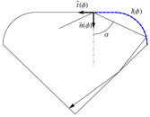
Figure 2: Variables of the reduced phase space. The blue dashed line represents $l(\phi)$ while $\alpha$ is the angle formed by the normal vector at position $\phi$, $n(\phi)$, and the trajectory of the particle after the impact.

We chose a rescaled arclength $l(\phi)$, and the angle $\alpha$ which defines the direction after the impact as the variables to describe the particle motion in the billiard. These variables are shown in Figure 2. The rescaled arclength is defined as $l(\phi)=\frac{L(\phi)}{L(2\pi)}$ where $L(\phi)=\int_{0}^{\phi}r_{c}(\phi)d\phi$. In order to compute the position and velocity of the $(n+1)$-th collision, using the position $\left(x^{(n)},y^{(n)}\right)=\left(r_{c}\left(\phi^{(n)}\right),\phi^{(n)}\right)$ and the incident velocity $\vec{v}^{(n)}=(v_{x}^{(n)},v_{y}^{(n)})$ of the $n$-th collision, we may proceed as follows: (i) Incident velocity of the (n+1) collision. The normal $v_{n}^{(n)}$ and tangent $v_{t}^{(n)}$ components of the velocity $\vec{v}^{(n)}$ are computed by projecting it into the normal, $\hat{n}(\phi)$, and the tangent, $\hat{t}(\phi)$, unitary vectors of the boundary. Just after the collision with the boundary the normal component velocity changes its sign while the tangent component remains unchanged, thus one can obtain the velocity $\vec{v}^{(n+1)}$ after the $n$-th collision which is also the incident velocity $(n+1)$-th collision. For this calculation the components of the tangent vector $\vec{t}=\frac{d}{d\phi}\left(r_{c}(\phi)\cos\phi,r_{c}(\phi)\sin\phi\right)=\left(T_{x},T_{y}\right)$ are needed. These are

$$T_{x}(\phi)=\left\{\begin{array}[]{ll}-r_{+}(\phi)\sin\phi+\cos\phi w_{+}(\phi)&\mbox{ if $\phi_{A}<\phi<\phi_{B}$ }\\ -R&\mbox{ if $\phi_{B}<\phi<\phi_{C}$}\\ -r_{-}(\phi)\sin\phi+\cos\phi w_{-}(\phi)&\mbox{ if $\phi_{C}<\phi<\phi_{D}$}\\ \left(R+d_{1}/2\right)a&\mbox{ if $\phi_{D}<\phi<2\pi$}\end{array}\right.$$ (7)

and

$$T_{y}(\phi)=\left\{\begin{array}[]{ll}r_{+}(\phi)\cos\phi+\sin\phi w_{+}(\phi)&\mbox{ if $\phi_{A}<\phi<\phi_{B}$ }\\ 0&\mbox{ if $\phi_{B}<\phi<\phi_{C}$}\\ r_{-}(\phi)\cos\phi+\sin\phi w_{-}(\phi)&\mbox{ if $\phi_{C}<\phi<\phi_{D}$}\\ -d_{2}a&\mbox{ if $\phi_{D}<\phi<\phi_{E}$}\\ d_{2}a&\mbox{ if $\phi_{E}<\phi<2\pi$}\end{array}\right.$$ (8)

where

$$w_{\pm}(\phi)=\mp\frac{1}{2}d_{1}\sin\phi\left(1\pm\frac{d_{1}\cos\phi}{2r_{\pm}(\phi)\mp d_{1}\cos\phi}\right)$$ (9)

and

$$a=\frac{1}{\sqrt{\left(R+\frac{d_{1}}{2}\right)^{2}+d_{2}^{2}}}.$$ (10)

The normal vector is obtained by rotating the tangent vector $\hat{n}=\mathbb{R}(-\pi/2)\hat{t}$, hence $n_{x}(\phi)=t_{y}(\phi)$ and $n_{y}(\phi)=-t_{x}(\phi)$. (ii) Position of the $(n+1)$-th collision. If the line which crosses through the points $\left(x^{(n)},y^{(n)}\right)$ and $\left(x^{(n+1)},y^{(n+1)}\right)$ is $Y^{(n)}(x)=m^{(n)}x+b^{(n)}$, then the slope and the $y$-intercept are

$$m^{(n)}=\frac{v_{y}^{(n)}}{v_{x}^{(n)}}\hskip 14.22636pt\mathrm{and}\hskip 14.22636ptb^{(n)}=y^{(n)}-\frac{v_{y}^{(n)}}{v_{x}^{(n)}}y^{(n)}\,,$$ (11)

respectively. The intersections of a line $Y(x)=mx+b$ with the boundary are

$$x^{*}_{i}=\left\{\begin{array}[]{rl}x_{+}^{\pm}&\mbox{ if $\frac{d_{1}}{2}<x_{+}^{\pm}\leq\frac{d_{1}}{2}+R$ and $Y(x_{+}^{\pm})>0$}\\ \frac{R-b}{m}&\mbox{ if $|\frac{R-b}{m}|\leq\frac{d_{1}}{2}$ and $Y(\frac{R-b}{m})>0$}\\ x_{-}^{\pm}&\mbox{ if $-R-\frac{d_{1}}{2}<x_{-}^{\pm}\leq-\frac{d_{1}}{2}$ and $Y(x_{-}^{\pm})>0$}\\ x_{+}&\mbox{ if $-R-\frac{d_{1}}{2}<x_{+}<0$ and $Y(x_{+})<0$}\\ x_{-}&\mbox{ if $0<x_{-}<R+\frac{d_{1}}{2}$ and $Y(x_{-})<0$}\end{array}\right.$$ (12)

where we have defined

$$x_{\pm}=\mp\frac{(b+d_{2})(d_{1}+2R)}{2d_{2}\pm m(d_{1}+2R)}\hskip 28.45274pt\mbox{and}$$ (13)

$$x_{s}^{\pm}=\frac{s\hskip 2.84544ptd_{1}-2bm\pm\sqrt{4(1+m^{2})R^{2}-(d_{1}m+2b)^{2}}}{2(1+m^{2})}$$ (14)

with $s=\left\{+,-\right\}$. The diamond billiard is a convex billiard, so the equation (12) gives us two roots: $x^{*}_{1}$ and $x^{*}_{2}$, one of them is the position of the current collision so it is known, let us call it $x^{n}=(x^{*}_{1})^{(n)}$, the other root gives the position of the $(n+1)$ collision

$$x^{(n+1)}=(x^{*}_{2})^{(n)}\hskip 14.22636pt\mathrm{and}\hskip 14.22636pty^{(n+1)}=Y^{(n)}\left((x^{*}_{2})^{(n)}\right).$$ (15)

Figure 3: Several trajectories after 1000 collisions are plotted. (Upper panel) $\xi=1-1\times 10^{-16}$, note that regular behaviour is obtained only for values of $\zeta$ very close to 1. (Middle panel) Some closed orbits of the triangular billiard. (Lower panel) For $\xi$ far enough from 1 (diamond billiards), the trajectory fills the billiard irregularly (left) $\xi=0.99$ and (right) $\xi=0$.

In general this procedure works well. Nonetheless, if the particle reaches one of the points $\left\{A,B,C,D,E\right\}$ where the tangent and normal vectors to the boundary are not defined, then the method fails. Although, this situation for an arbitrary initial condition rarely happens, the problem sometimes is solved by taking the average of the normal and tangent vectors for the boundaries connected in those problematic points. In Figure 3 are shown some trajectories for the triangular billiard and the diamond billiard using the procedure described above.

2.1.1 Entropy

In the previous section, a methodology based on geometry was used to find the classical trajectories of the particle in a diamond billiard. Indeed, this is not the more elegant way to find trajectories, and there should exist a transformation or map which connects the variables of the reduced phase space of consecutive collisions of the diamond billiard. In principle, the trajectories of the particle may be constructed with the knowledge of the billiard map and the initial conditions. If we avoid the very special cases of the periodic orbits, then the degree of irregularity of a set of trajectories with different initial conditions should depend only on the shape of the billiard. The entropy $S$ is calculated in order to determine quantitatively such degree of irregularity. $S$ may be computed as follows: Let $\alpha_{n}$ be the incident angle with respect the normal vector on the boundary. The range of this variable is the interval $I=[-\pi/2,\pi/2]$. This interval is divided in $M$ equal subintervals $I_{i}$. Then $N$ collisions and their respective incident angles $\alpha_{n}$ are generated, where $n=1,2,3,..,N$. If $N_{i}$ is the number of angles $\alpha_{n}$ which live in the interval $I_{i}$, then the probability to find an incident angle in the interval $I_{i}$ is $P\left(I_{i}\right)=\frac{N_{i}}{N}$, and the entropy $S$ may be computed in the standard way as

$$S=-\sum_{i=1}^{N}P\left(I_{i}\right)\ln\left[P\left(I_{i}\right)\right].$$ (16)

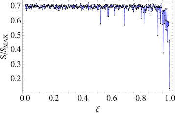
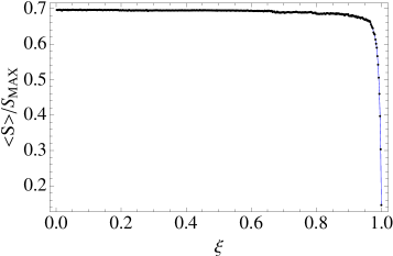
Figure 4: Entropy. (left) Entropy computed for a single value of $\xi$ and one initial random condition. The number of collisions of these graphs were $N=3000$, and the interval subdivisions were $M=100$. (right) We have generated 1000 random initial conditions with their respective entropies, and later these entropies were averaged.

The maximum entropy is obtained when the set of generated incident angles $\left\{\alpha_{n}\right\}$ are uniformly distributed in the subintervals $\left\{I_{i}\right\}$. For this case the probability is equal for each subinterval, hence $P\left(I_{i}\right)=\frac{1}{N}$, and the entropy takes its maximum value $S_{max}=\ln(N)$. On the other hand, if all incident angles lie in a single subinterval $I_{j}$, then the probability would be $P\left(I_{i}\right)=\delta_{ij}$, and the entropy is zero. The entropy computation using the equation (16) generally depends on the initial condition used. In order to avoid this dependence we have computed the entropy for 1000 trajectories with different random initial conditions. Posteriorly, these entropies were averaged for each particular value of the control parameter (Figure 4). The smallest value of entropy is obtained when $\xi$ is exactly one and the billiard is an equilateral triangle. The entropy grows quickly as the half of stadium is introduced in one of the triangle sides, even when the control parameter is close to one as $\xi=0.99$ where the corresponding entropy is about the $55\%$ of its maximum theoretical value. As $\xi$ is set far from one, the entropy practically stabilizes its value reaching about a $70\%$ of $S_{max}$. In this regime, the trajectory of the particle is more complex than the one found for $\xi$ close to one as it is clear from a comparison between the lower and upper panels of Figure 3.

2.1.2 Lyapunov exponent

The Lyapunov exponent $\lambda$ is used as a measure of divergence between trajectories for a couple of infinitesimal close initial conditions in the phase space. The time is not a suitable parameter in order to compute $\lambda$ in billiard systems since the particle movement is linear while it does not collide and the trajectories will diverge linearly. The collision index $n$ was used as parameter instead of time, as usual a great sensibility with small changes of the initial conditions is characterized by $\delta_{n}=\delta_{o}\exp\left(\lambda n\right)$ where $\delta_{n}$ is the absolute value of the difference between incident angles of nearby trajectories after $n$ collisions.

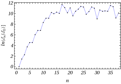
Figure 5: Lyapunov exponent saturation. This is a typical graphic obtained for a single value of the control parameter ($\xi=0.9999$) and one random initial condition; 40 collisions are considered. For this particular situation the saturation occurs about after 13 collisions. The Lyapunov exponent is the slope of the non-saturated part.

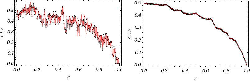
Figure 6: Averaged Lyapunov exponent. The number of random initial conditions of each graph was (left) 10 and (right) 1000.

The Lyapunov exponent was averaged in order to avoid the dependence with the initial conditions. For a couple of close trajectories random initial conditions were generated, and the Lyapunov exponent was computed for each initial condition (Figure 5). The Lyapunov exponents computed in the previous step were averaged for each value of $\xi$ (Figure 6). In order to minimize the error introduced by the saturation, we decided to calculate the slope between adjacent points and average it for each single Lyapunov exponent computed, thus the saturated points frequently have small contribution due to the alternation of the slope sign. Some graphics are not well defined as the one shown in Figure 6 and some inaccuracies persist in the final result, even if the number of initial conditions is increased. For this reason, the final averaged on the Lyapunov exponent in Figure 6 is not as smooth as the entropy of the Figure 5. However, the Figure 6 is able to capture an important feature of the billiard: as the half stadium appears over one side of the original equilateral triangle, then the Lyapunov exponent substantially increases, and the non negative values of it ensures a great sensibility to the initial conditions, even for values of $\xi$ close to one.

3 Quantum diamond billiard: Finite Difference Method Implementation

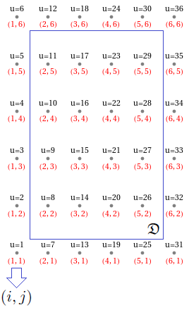
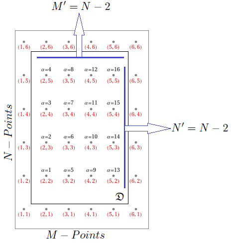
Figure 7: First and second indexing. (left) The domain is discretized in a rectangular lattice of $M\times N$ points including the boundary (the points out the solid rectangle). Each point $(i,j)$ is labelled by the single index $u$. (right) Here only the inner points are indexed, we build the map $\alpha=\alpha(i,j)$, inversely the pair $(i,j)$ is obtained by $i=i_{2}(\alpha)$ and $j=j_{2}(\alpha)$. The points of the two indexing are related by $u=u(i,j)=u\left(i_{2}(\alpha),j_{2}(\alpha)\right)$. The total number of inner points is $Q=M^{\prime}\times N^{\prime}$

This problem is typically solved by using finite element method (FEM) and iterative methods on the discretized version of the Schrödinger equation [2]. We may use the FDM to express the Hamiltonian as a matrix on a lattice, and then solve the resulting eigenvalue problem. The discretization of the region is shown in Figure 7-left, each point at the position $\vec{r}_{ij}$ is labelled in one of these ways: with pair $(i,j)$ or the single index $u$. The second option is used in order to avoid the impractical use of four indices in the Hamiltonian matrix. During the lattice construction it is easy to build the function $u=u(i,j)$ which maps from the pair of indices $(i,j)$ to the point $u$, let us call this process as the first indexing. The time independent Schrödinger equation is evaluated at the point $u(i,j)$ according to

$$-\left.\frac{\hbar}{2m}\vec{\nabla}^{2}\psi(\vec{r})\right|_{u(i,j)}+\left.V(\vec{r})\psi(\vec{r})\right|_{u(i,j)}=E\left.\psi(\vec{r})\right|_{u(i,j)}.$$ (17)

The second derivatives of the laplacian may be evaluated using central differences [3]

$$\left.\frac{\partial^{2}\psi}{\partial x^{2}}\right|_{u(i,j)}\approx\frac{1}{\delta x^{2}}\left[\psi_{u(i+1,j)}+\psi_{u(i-1,j)}-2\psi_{u(i,j)}\right]$$

and

$$\left.\frac{\partial^{2}\psi}{\partial y^{2}}\right|_{u(i,j)}\approx\frac{1}{\delta y^{2}}\left[\psi_{u(i,j+1)}+\psi_{u(i,j-1)}-2\psi_{u(i,j)}\right].$$

The notation is simplified defining

$$u^{\pm}=u\left(i(u)\pm 1,j(u)\right).$$ (18)

This transformation makes a horizontal displacement in the lattice from the point $u$. Although, there are several values of $u$ for a single $i$ or $j$ ($N$ values for the index $i(u)$, and $M$ values for the index $j(u)$) we have only one value for $u$ fixing both $i$ and $j$. The equation (18) gives the neighbor of $u$ at its left $(-)$ or right $(+)$. Similarly, the vertical displacement from the point $u(i,j)$ is computed with

$$u_{\pm}=u\left(i(u),j(u)\pm 1\right)\,.$$ (19)

With this notation, equation (17) may be written as

$$\sum_{v\in\mathfrak{D}}H_{uv}\psi_{v}=E\psi_{u}\hskip 28.45274pt\mbox{where}$$

$$H_{uv}=-\frac{\hbar^{2}}{2m}\left[\frac{\delta_{u^{+},v}+\delta_{u^{-},v}}{\delta x^{2}}+\frac{\delta_{u_{+},v}+\delta_{u_{-},v}}{\delta y^{2}}-2\delta_{u,v}(\delta x^{-2}+\delta y^{-2})\right]+V_{u}\delta_{u,v}$$ (20)

is the Hamiltonian (repeated indices in the last term do not involve sum over them). Since the problem is solved only for the inner points, we performed a second indexing (see Figure 7-right), so the eigenvalue equation may be written as

$$\sum_{v\in\mathfrak{D}}H_{uv}\psi_{v}=\sum_{\beta=1}^{Q=M^{\prime}\times N^{\prime}}H_{u(\alpha)v(\beta)}\psi_{v(\beta)}=E\psi_{u(\alpha)}.$$ (21)

The eigenvalues and eigenvectors of the Hamiltonian $H_{\alpha\beta}$ are obtained numerically. Commonly, the packages of matrix diagonalization arrange the eigenvectors in a matrix, let us call it $M_{\alpha\beta}$

$$M=\left({\begin{array}[]{*{20}c}M_{11}&M_{12}&\cdots&M_{1Q}\\ M_{21}&M_{22}&\cdots&M_{2Q}\\ \vdots&\vdots&\vdots&\vdots\\ M_{Q1}&M_{Q2}&\cdots&M_{QQ}\end{array}}\right).$$ (22)

If the eigenvectors are arranged in the columns of such matrix, then the state $s$ evaluated at the point $\alpha$ is $\psi_{\alpha}^{(s)}=M_{\alpha s}$ with $(s=1,2,...,Q)$. In order to return to the initial labelling we may write

$$\psi_{ij}^{(s)}=\left\{\begin{array}[]{rl}M_{\alpha(i,j),s}&\hskip 14.22636pt\mathrm{if}\hskip 14.22636pt\vec{r}_{ij}\in\mathfrak{D}\\ 0&\hskip 14.22636pt\mathrm{otherwise.}\end{array}\right.$$ (23)

The generalization for billiards of arbitrary shape does not represent considerable difficulties. We may place the boundary of the arbitrary shape billiard over the rectangular grid and take only the points inside of it. After the identification of the boundary points, the inner points (say $Q$ inner points) are enumerated first $(u=1,2,...,Q)$, and the boundary points later, so a second indexation is avoided. Some grids for the billiard consider in this study are shown in Figure 8.

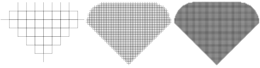
Figure 8: The grid. As the density of points is incremented, the mesh is better adjusted to the geometry of the billiard. Some grids are shown, the number of inner points are: (left) $Q=32$, (center) $Q=1108$ and (right) $Q=4618$.

Table 1: Triangular billiard eigenvalues.

State	$E_{n}$ (J)	$E_{n}$ (J)	Relative Error
$n$	FDM	Exact	$\%$
1	2.14940	2.14849	0.04235
2	5.01655	5.01313	0.06817
3	5.01743	5.01313	0.08570
4	8.59995	8.59394	0.06988
5	9.31609	9.31010	0.06429
6	9.31662	9.31010	0.06998
7	13.6095	13.6071	0.01763
8	13.6171	13.6071	0.07343
9	15.0451	15.0394	0.03788
10	15.0451	15.0394	0.03788
11	19.3386	19.3364	0.01137
12	20.0559	20.0525	0.01695
13	20.0559	20.0525	0.01695
14	22.1997	22.2010	0.00585
15	22.2001	22.2010	0.00405

The numerical results were compared with the exact ones for the equilateral triangular billiard. The triangular billiard is integrable and the expression for the energy levels is well known [4]

$$E_{n}=E_{pq}=\left(\frac{4\pi}{3}\right)^{2}\left(\frac{\hbar^{2}}{2md_{1}^{2}}\right)\left(p^{2}+q^{2}-pq\right)$$ (24)

where $d_{1}$ is the edge length when $\xi=1$, $p$ and $q$ are positive integers which satisfy $q\in\left[1,p/2\right]$. A comparison of the numerical and analytic energy levels was done and listed in Table 1. One advantage of the FDM lies in the fact that Hamiltonian is computed by a direct evaluation of the potential and some Kronecker deltas, so in a personal computer (in our case an i7 processor) building a Hamiltonian matrix of $11000\times 11000$ take less than a minute, and its orthogonalization with the lapack package using Fortran, requires about 25 minutes. In order to check the accuracy of the results, a comparison with the energy staircase function $\mathcal{N}(E)$ with the Weyl-type formula was performed. $\mathcal{N}(E)$ gives the number of energy levels under the energy $E$ and it is defined by

$$\mathcal{N}(E):=\sum_{i}\theta\left(E-E_{i}\right)$$ (25)

where $\theta(x)$ is the step function. The analytical result for a two-dimensional billiard with area $A$ and perimeter $P$ is given by [5, 6, 7, 8]

$$\mathcal{N}(E)=\frac{A}{4\pi}\left(\frac{2mE}{\hbar^{2}}\right)-\frac{P}{4\pi}\sqrt{\frac{2mE}{\hbar^{2}}}+o(E^{1/2}).$$ (26)

Carefully speaking, the Weyl formula is valid in the semiclassical limit, that is for high energy levels.

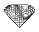
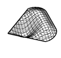
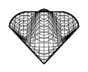
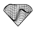
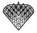
Figure 9: Diamond shape billiard wavefunctions. Here some eigenfunctions are plotted using the a grid with $Q=4618$ inner points (see Figure 8), and the control parameter was set as $\xi=1$. We have set $m=1$ and $\hbar=1$.

Other typical problems in billiards as the scar identification deep in the semiclassical limit may be faced using more convenient methods. For instance, the improved Heller’s PWDM (Heller’s plane wave decomposition method) [9]. This method avoids the computation of the eigenvectors near to the ground state and goes directly for the computation of the states with high quantum numbers. We used the finite difference method in order to diagonalize quantum diamond billiard. Some of the first excited states of this billiard are shown in Figure 9. In Figure 10 we have superposed the numerical result of the energy staircase function with the one provided by (26). The deviation of the numerical results to the theoretical prediction for high energies is due to numerical errors because the discretization procedure is not able to describe properly wavefunctions corresponding to very high energies, which have very small wavelength oscillations. From this, it is clear that only the first $\sim 200$ computed states are reliable.

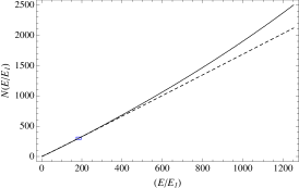
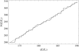
Figure 10: Spectral staircase function for the diamond shaped billiard. (left) Superposition of the numerical staircase energy staircase function (solid line), with the Weyl’s formula (dashed line). (right) A zoomed region corresponding to the blue rectangle of the graphic on the left side.

4 Quantum diamond billiard: level statistics

Several experiments were performed in the nineties with quantum hard wall billiards, e.g. the microwave resonators, which used the equivalence between the stationary Scrödinger equation with the Helmholtz equation to study chaos in quantum billiards using electromagnetic waves [10]. Other devices used in the quantum chaos study were the semiconductors billiards, those are open quantum cavities which permit a current flow through two contact points. These structures are different from a quantum billiard, which is completely closed and confines a single particle inside it. However, if the size of the quantum open cavity is much smaller than the mean free path of the electrons, then the device approaches a quantum billiard and it shares with the quantum billiards several properties e.g. energy level statistics and the scarring of the wavefunction [2]. For Hamiltonian systems such as the one described in this writing the energy level spacing distribution, $P(s)$, is a feature which distinguishes the spectrum of a system with regular or chaotic classical analogue. According to the Bohigas-Giannoni-Schmit conjecture [11] the spectra of a time-reversal-invariant system with a classical chaotic counterpart follows a Gaussian Orthogonal Ensamble (GOE) distribution. On the other hand, if the classical analogue is regular, then the spectrum is characterized by a Poisson distribution (see Figure 11). This conjecture has been tested in a variety of systems including billiards.

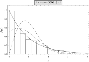
Figure 11: Nearest neighbor spacing distribution of the energy levels of the triangular billiard. The histogram was built using the analytic expression for the energy levels of the equilateral triangular billiard (see equation (24)). The level statistics is Poissonian (solid line) because the equilateral triangle billiard is regular. For the irregular case, the nearest neighbor spacing distribution will follow either a GOE2 distribution (dashed line) or a GOE distribution (dot dashed line) according to the billiard symmetries.

The diamond shaped billiard has a mirror reflection symmetry axis. For this reason, there are two set of states related to each symmetry class, namely, odd or even eigenstates. The general expression of the nearest neighbour spacing distribution for a superposition of $N$ independent spectra in the GOE statistics is given by [12]

$$P_{N\,\mathrm{GOE}}(s)=\frac{\partial^{2}}{\partial s^{2}}\left[\mathrm{erfc}\left(\frac{\sqrt{\pi}s}{2N}\right)\right]^{N}$$ (27)

where $s$ is the energy spacing between nearest neighbour levels, and $\mathrm{erfc}(x)$ is the complementary error function. The spacing distribution for $N=2$ is

$$P_{2\,\mathrm{GOE}}(s)=\frac{1}{2}e^{-\frac{s^{2}\pi}{8}}+\frac{\pi s}{8}e^{-\frac{s^{2}\pi}{10}}\mathrm{erfc}\left(\frac{\sqrt{\pi}s}{4}\right).$$ (28)

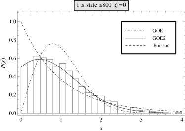
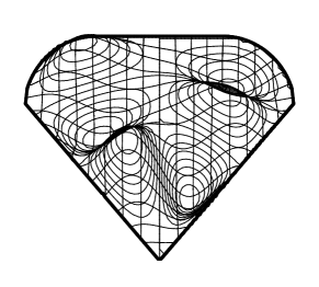
Figure 12: Nearest neighbor spacing distribution of the complete billiard. (left) The histogram of the level spacing distribution was built using the first 800 energy levels, the first one hundred states were not taken. The total number of energy levels computed using the finite difference method was $Q=11026$. (right) Ninth state of the complete diamond shaped billiard.

In Figure 12 it is shown the nearest neighbor spacing distribution of the diamond shaped billiard which fits the $P_{2GOE}$ (GOE2) distribution, as expected.

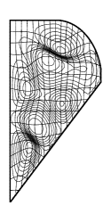
Figure 13: Nearest neighbor spacing distribution of the desymmetrized diamond shaped billiard. (left) The histogram of the level spacing distribution was built using the first 500 energy levels. The total of energy levels computed using the finite difference method was $Q=11252$. (right) Ninth state of the desymmetrized diamond shaped billiard.

There are two ways to recover the GOE distribution: the first one is to classify the energy levels according to the parity of the eigenstates and the histogram is built with one of the two sets. However, there is a disadvantage in this method, because it requires to take approximately the half of the energy levels computed. The second one consists in statistical study of the corresponding desymmetrized billiard spectrum. In this case the billiard is desymmetrized by taking a half of it for the mirror symmetry of the diamond billiard. The level statistic effectively obeys a GOE distribution for the desymmetrized billiard. The result is shown in Figure 13.

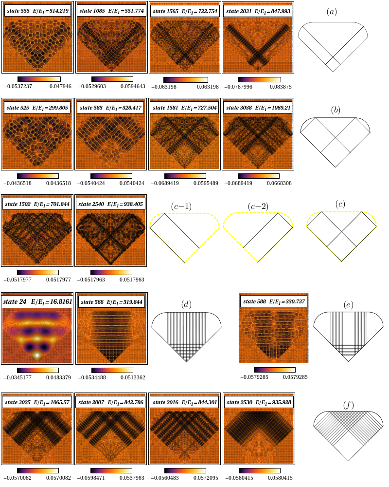
Figure 14: Some scarred wavefunctions and bouncing ball states of the diamond shaped billiard.

Another important feature of quantum chaotic billiards is the high concentration of the wavefunction amplitude along the classical periodic orbits. The phenomenon was initially observed by McDonald and Kaufman [13], and posteriorly in the Bunimovich billiard by Heller [14], who called it a scar. Using the analytic solution of the wavefunction it is not possible to built a scar in the rectangular, circular or equilateral triangle billiard. The scarring of wavefunction in billiards does not appear in regular billiards, and it is exclusive for the chaotic ones. As the quantum numbers are increased, we expect to recover the classical characteristics of the system, which is, in some sense, the idea behind the correspondence principle. In a chaotic billiard, the trajectories which evolve from an arbitrary initial condition tend to fill the whole billiard, as consequence a typical wavefunction should not have a significant localization, which is the more common situation for the irregular billiards. Nonetheless, for the special case of an unstable periodic orbit, it is possible to find a high probability density underlying such classical trajectory, as we may intuitively expect at least in the semiclassical limit. Some scars and bouncing ball states are shown in Figure 14. The bouncing ball states have a well defined momentum, but not position and we may associate a set of classical periodic orbits to a single bouncing ball state. In contrast, a scar is related to a single unstable periodic orbit.

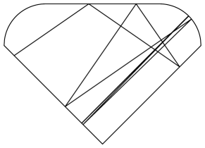
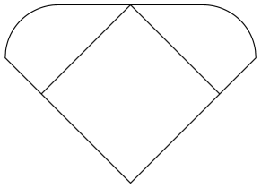
Figure 15: Orbits stability. (left) Unstable periodic orbit after 35 collisions, (right) stable periodic orbit after 1000 collisions.

Example of scars are shown in Figure 14-(a) and 14-(c). The stability of the orbits with lowest period is shown in Figure 15.

5 Quantum diamond billiard: time evolution of the state vector

In this section the study will be limited to the time evolution of the mean values. The time evolution of the state vector for quantum Hamiltonian systems is well known $\mid\Psi\left(t\right)\rangle=e^{-i\frac{\hat{H}t}{\hbar}}\mid\Psi\left(0\right)\rangle.$ Expanding the state vector over the corresponding stationary states $\mid\Psi\left(\vec{r},0\right)\rangle=\sum_{s}c_{s}\mid\psi^{(s)}\rangle$, and evaluating on one arbitrary inner point of the lattice we find

$$\left.\langle{\vec{r}}\mid\Psi\left(t\right)\rangle\right|_{\vec{r}=\vec{r}_{u}}=\Psi_{u}(t)=\sum_{s}c_{s}\exp{\left(-\frac{iE_{s}t}{\hbar}\right)}\psi^{(s)}_{u}.$$

The components are given in the usual way, however we may use the lattice in order to compute them easily

$$c_{s}=\lim_{\delta^{2}\vec{r}\to 0}\sum_{u\in\mathfrak{D}}\psi^{(s)}_{u}\Psi_{u}(0)\delta^{2}\vec{r}.$$ (29)

Since the eigenvectors of the Hamiltonian matrix, given by the equation (20), are real, then the complex conjugation has been dropped. If the number of inner points is large, we may use the last equation without the limit as a good approximation for the components computation. The same approach may be used for the computation of the several mean values involved in the uncertainty products for momentum and position. Using the index displacement transformations and central differences, the gradient evaluated at the point $u(i,j)$ may be expressed as

$$\left(\vec{\nabla}\Psi\right)_{u}=\frac{1}{2}\left(\frac{\Psi_{u^{+}}(t)-\Psi_{u^{-}}(t)}{\delta x},\frac{\Psi_{u_{+}}(t)-\Psi_{u_{-}}(t)}{\delta y}\right)\hskip 2.84544pt,$$ (30)

so the mean value for momentum takes the form

$$\langle\hat{\vec{p}}(t)\rangle=\frac{\hbar}{i}\lim_{\delta^{2}\vec{r}\to 0}\sum_{u\in\mathfrak{D}}\Psi_{u}(t)^{*}\left(\vec{\nabla}\Psi\right)_{u}\delta^{2}\vec{r}.$$ (31)

Taking the real and imaginary part of the last equation we find

$$\langle\hat{\vec{p}}(t)\rangle=\hbar\lim_{\delta^{2}\vec{r}\to 0}\sum_{u\in\mathfrak{D}}\left[\vec{\nabla},\Psi\right]_{u}(t)\delta^{2}\vec{r}$$

and

$$\lim_{\delta^{2}\vec{r}\to 0}\sum_{u\in\mathfrak{D}}\left\{\vec{\nabla},\Psi\right\}_{u}(t)\delta^{2}\vec{r}=0$$ (32)

where the following expressions were defined

$$\begin{array}[]{l}\displaystyle\left[\vec{\nabla},\Psi\right]_{u}(t):=\mathrm{Re}\left[\Psi_{u}(t)\right]\mathrm{Im}\left[\left(\vec{\nabla}\Psi\right)_{u}(t)\right]-\mathrm{Im}\left[\Psi_{u}(t)\right]\mathrm{Re}\left[\left(\vec{\nabla}\Psi\right)_{u}(t)\right]\mbox{ and }\vspace{0.5cm}\\ \displaystyle\left\{\vec{\nabla},\Psi\right\}_{u}(t):=\mathrm{Re}\left[\Psi_{u}(t)\right]\mathrm{Re}\left[\left(\vec{\nabla}\Psi\right)_{u}(t)\right]+\mathrm{Im}\left[\Psi_{u}(t)\right]\mathrm{Im}\left[\left(\vec{\nabla}\Psi\right)_{u}(t)\right].\end{array}$$ (33)

The condition in the equation (32) appears because the mean value is a real quantity, then for practical means, the imaginary part may be used to check the accuracy of the numerical integral evaluation. Similarly, for the mean value of the squared momentum we find

$$\langle\hat{\vec{p}}^{\hskip 1.42271pt2}(t)\rangle=-\hbar^{2}\lim_{\delta^{2}\vec{r}\to 0}\sum_{u\in\mathfrak{D}}\left\{\vec{\nabla}^{2},\Psi\right\}_{u}(t)\delta^{2}\vec{r}$$ (34)

with

$$\lim_{\delta^{2}\vec{r}\to 0}\sum_{u\in\mathfrak{D}}\left[\vec{\nabla}^{2},\Psi\right]_{u}(t)\delta^{2}\vec{r}=0$$

where the laplacian at the point $u(i,j)$ is

$$\left(\vec{\nabla}^{2}\Psi\right)_{u}=\frac{\Psi_{u^{+}}(t)+\Psi_{u^{-}}(t)}{\delta x^{2}}+\frac{\Psi_{u_{+}}(t)+\Psi_{u_{-}}(t)}{\delta y^{2}}-2(\delta x^{-2}+\delta y^{-2})\Psi_{u}(t).$$ (35)

Finally, the average of an arbitrary function $f$ with only position dependence is

$$\langle f(\hat{\vec{r}})\rangle(t)=\lim_{\delta^{2}\vec{r}\to 0}\sum_{u\in\mathfrak{D}}\mid\Psi_{u}(t)\mid^{2}f_{u}.$$ (36)

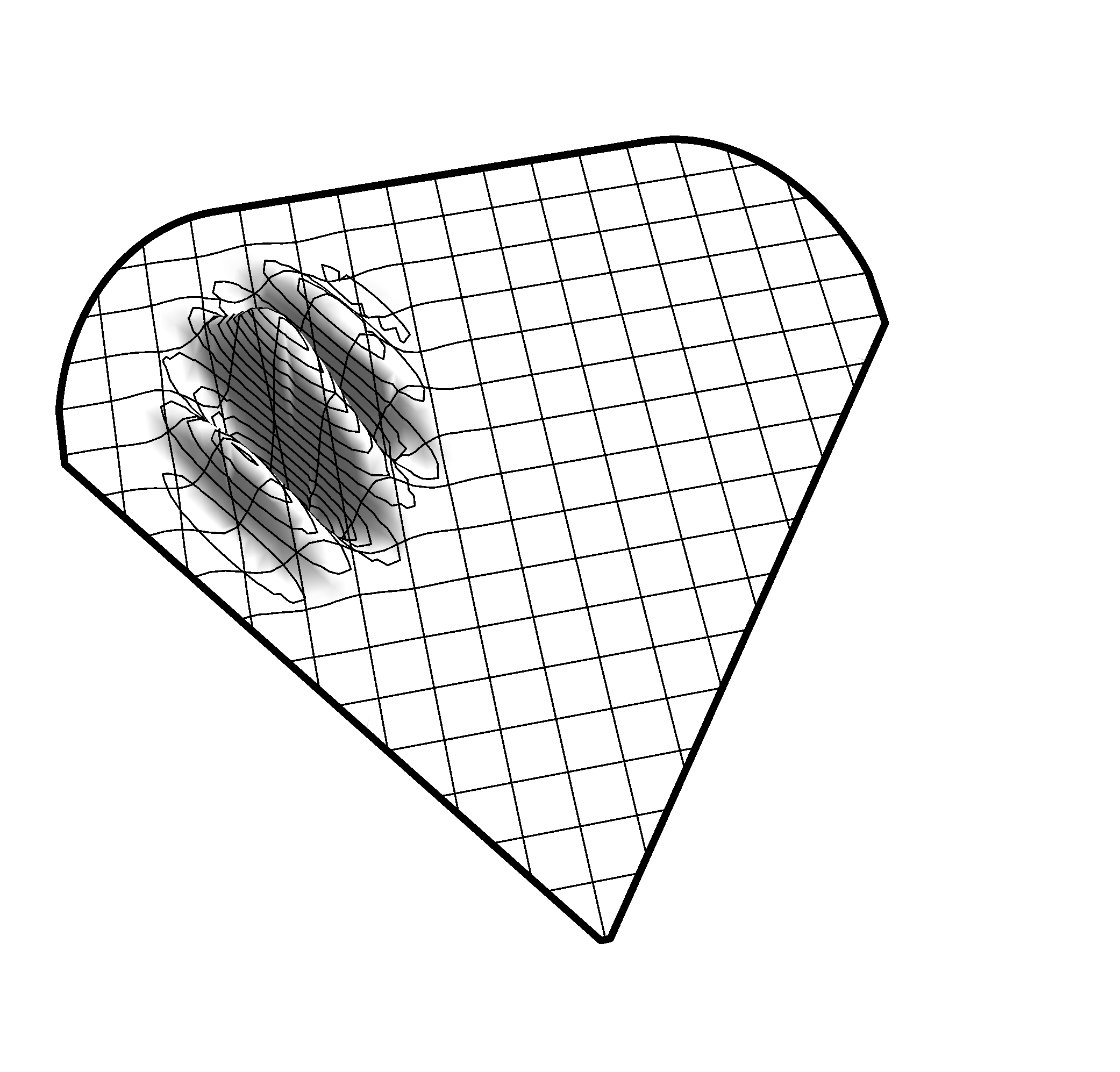
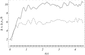
Figure 16: Gaussian wave packet evolution. (Top). (left) Initial state. (right) Uncertainty products: $\Delta x\Delta p_{x}$ (solid line) and $\Delta y\Delta p_{y}$ (dashed line). The dot dashed line is the minimum uncertainty value $\Delta x\Delta p_{x}=\hbar/2$ (dot-dashed line). (Bottom). Trajectory of the position operator expectation values.

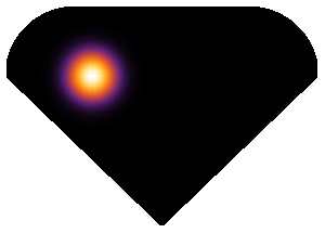
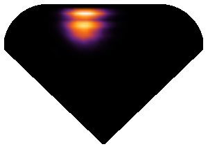
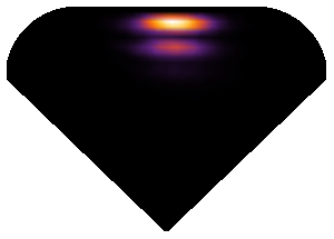
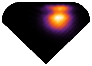
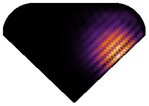
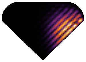
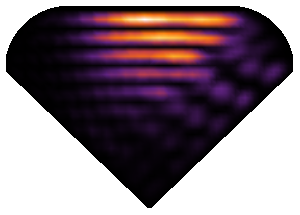
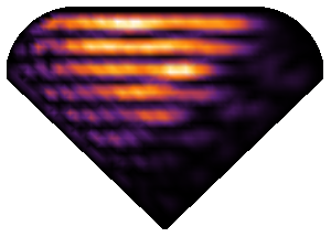
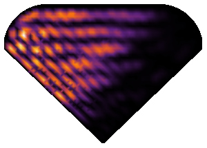
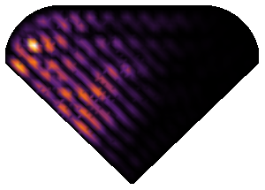
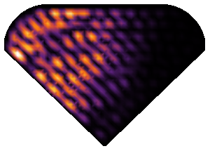
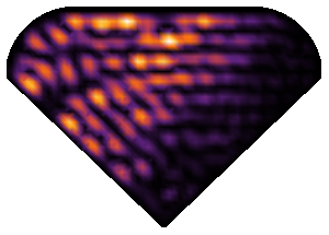
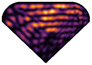
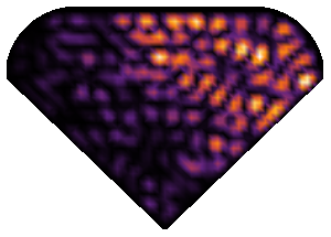
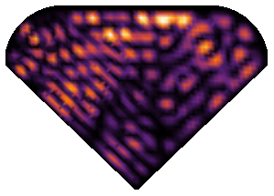
Figure 17: Probability density distribution of the billiard prepared in a Gaussian wave packet. The packet was initially placed in $\vec{r}_{o}=(-R,0)$. The wave vector was pointed to $\pi/4$ rad respect the $x$-axis. Classically, the particle should describe the 4-periodic orbit shown in Figure 15; nonetheless, after the second collision the corresponding state is highly delocalized. The particle tends to remain on a bouncing ball state after the second collision (see Figure 14-(f)); however, the next collisions increase the delocalization and the evolution turns non-coherent.

The time evolution of the position mean values of the system prepared in a well localized initial state at $\vec{r}_{o}=(x_{o},y_{o})$ using a Gaussian wave packet

$$\langle\vec{r}\mid\Psi(0)\rangle=\frac{e^{-\frac{(x-x_{o})^{2}}{4\sigma_{x}^{2}}-\frac{(y-y_{o})^{2}}{4\sigma_{y}^{2}}+i\left(\kappa_{x}x+\kappa_{y}y\right)}}{2\pi\sigma_{x}\sigma_{y}}$$ (37)

is shown in Figure 16. $\vec{\kappa}=(\kappa_{x},\kappa_{y})$ is the wave vector, $\sigma_{x}$ and $\sigma_{y}$ are the standard deviation on along $x$ or $y$ respectively. As seen in Figure 17, the wavepacket is destroyed after a few collisions. However, this is not a consequence of the classical chaotic behaviour and such irregular dynamics may be attributed to a non-coherent preparation of the initial state. This is checked in the evolution of the uncertainty products. The system must be prepared in a coherent state in order to reduce the uncertainty products to their minimum value $\hbar/2$; nevertheless, we do not have a general analytical expression for the coherent states of billiards, even in simple cases such as a particle in a rectangular box.
Classical chaos of an specific system often emerges from its nonlinear nature. Nevertheless, the classical and quantum billiard systems are an exception of this rule because of the absence of nonlinear terms in their governing equations. Indeed, the difficulty for quantum chaos determination does not lie in this lack of nonlinearity rather the problem resides in the difficulty to find a correspondence between the classical and quantum behaviour far from the classical limit when the classical system evolves chaotically. The question is not solved by simply proving the Bohigas-Giannoni-Schmit conjecture because the nearest neighbor spacing distribution is just a semiclassical result. The analysis of the position operator expectation value is an alternative to study the correspondence between the classical and quantum system in an irregular regime. However, this approach frequently is not successful because the quantum system evolves in a non-coherent way when its classical counterpart is chaotic as we show in this writing. This would be reason, for which the quantum Hamiltonian system sensibility has been sometimes studied by perturbing the Hamiltonian instead of by changing the initial state [15].

6 Concluding remarks

The classical and quantum diamond billiard was studied through some quantities. In particular, we calculate the entropy, the Lyapunov exponent and some trajectories for the classical problem. The classical chaotic behaviour emerges fast with small modifications on the boundary of the regular equilateral billiard ($\xi=1$). The entropy and the Lyapunov exponent grow when a half of stadium is introduced in one side of the triangular billiard. If the control parameter is set far enough from one, say in the interval $0.8\leq\xi\leq 1$, then the entropy practically is a $70\%$ of $S_{max}$. This percentage is relative far from its maximum and it occurs because the diamond billiard does not have dispersive frontiers as other billiards e.g. Sinai billiard. Nonetheless, it is enough to ensure a great irregularity in the classical trajectories when the entropy is about $0.7S_{max}$.

The finite difference method provides a way to solve the quantum problem. The diamond shape billiard has a mirror reflecting symmetry. Because of this, the energy levels split in two different symmetry classes according to the wavefunction parity. As consequence, $P(s)$ for the complete billiard is given by a GOE2 distribution. If diamond billiard is desymmetrized, then the level statistics follows a GOE distribution. On the other hand, the classical behaviour is regular when the control parameter is set to one and the distribution is Poissonian. Therefore, the results are according to the Bohigas-Giannoni-Schmit conjecture. We found scarred states in the quantum diamond billiard, as well as bouncing ball states with their corresponding set of classical stable periodic orbits. These results are in agreement with previous work in the field for other Hamiltonian systems. In the last section, a practical way to compute the time evolution of the state vector was described and the lattice previously built in the finite difference method implementation was used for this aim.

References

- [1] M. L. Mehta, Random Matrices, Academic Press, 2d Ed. (2004)
- [2] R. Akis and D. K. Ferry, Wave Function Scarring Effects in Open Ballistic Quantum Cavities, VLSI Design, 8, 307 (1998)
- [3] R. Garg, Analytical and Computational Methods in Electromagnetics, Artech House, (2008)
- [4] M. Brack, R. Bhaduri Semiclassical Physics, Addison-Wesley Publishing Company, (1997)
- [5] H. Weyl, Göttingen Nach. 110 (1911)
- [6] H. Weyl, The Classical Groups: Their Invariants and Representations, Princeton university press (1946)
- [7] M. Kac, Can One Hear the Shape of a Drum?, Amer. Math. Month. 73, 1 (1966)
- [8] R. W. Robinett, Quantum mechanics of the two-dimensional circular billiard plus baffle system and half-integral angular momentum, Eur. J. Phys. 24 (2003) 231-243
- [9] B. Li and B. Hu, Statistical Analysis of Scars in Stadium Billiard J. Phys. A: Math. Gen. 31 483 (1998)
- [10] H. J. Stockman and D. K. Ferry, Chaos in Microwave resonators, Séminaire Poincaré IX, 1 (2006)
- [11] O. Bohigas, M. J. Giannoni, and C. Schmit, Characterization of Chaotic Quantum Spectra and Universality of Level Fluctuation Laws, Phys. Rev. Lett. 52, 1–4 (1984)
- [12] I. Kosztin and K. Schulten, Boundary Integral Method for Stationary States of Two-Dimensional Quantum Systems, Int. J. Mod. Phys. C 8, 293-325 (1997)
- [13] S. W. McDonald and A. N. Kaufman, Spectrum and eigenfunctions for a hamil- tonian with stochastic trajectories, Phys. Rev. Lett. 42 1189 (1979)
- [14] E. J. Heller, Bound-State Eigenfunctions of Classically Chaotic Hamiltonian Systems: Scars of Periodic Orbits, Phys. Rev. Lett. 53 1515 (1984)
- [15] D. A. Wisniacki, E. G. Vergini, H. M. Pastawski, and F. M. Cucchietti, Sensitivity to perturbations in a quantum chaotic billiard, Phys. Rev. E 65, 055206(R) (2002)