Confronting MOND and TeVeS with strong gravitational lensing over galactic scales: an extended survey

Abstract

The validity of MOND and TeVeS models of modified gravity has been recently tested by using lensing techniques, with the conclusion that a non-trivial component in the form of dark matter is needed in order to match the observations. In this work those analyses are extended by comparing lensing to stellar masses for a sample of nine strong gravitational lenses that probe galactic scales. The sample is extracted from a recent work that presents the mass profile out to a few effective radii, therefore reaching into regions that are dominated by dark matter in the standard (general relativity) scenario. A range of interpolating functions are explored to test the validity of MOND/TeVeS in these systems. Out of the nine systems, there are five robust candidates with a significant excess (higher that 50%) of lensing mass with respect to stellar mass, irrespective of the stellar initial mass function. One of these lenses (Q0957) is located at the centre of a galactic cluster. This system might be accommodated in MOND/TeVeS via the addition of a hot component, like a 2 eV neutrino, that contribute over cluster scales. However, the other four robust candidates (LBQS1009, HE1104, B1600, HE2149) are located in field/group regions, so that a cold component (CDM) would be required even within the MOND/TeVeS framework. Our results therefore do not support recent claims that these alternative scenarios to CDM can survive astrophysical data.

I Introduction

Over the past few years, it has been possible to test in detail the standard $\Lambda$CDM model of cosmology to new levels of accuracy, starting the so-called era of “precision cosmology”. Hitherto the model has been very successful at fitting observations (see e.g. teg06 ). This paradigm has as its foundation two main aspects: the application of classical general relativity in a homogeneous Friedmann-Lemaître-Robertson-Walker metric with positive cosmological constant $\Lambda$, along with the presence of a cold dark matter component (CDM). However, the nature of the cosmological constant and the type of dark matter species required are presently unknown and have been the focus of vigorous investigation for decades.

In the absence of any direct detection of CDM or a fundamental theory of $\Lambda$, proposals have been put forward which go beyond the framework of $\Lambda$CDM and offer possible alternative approaches to fitting observations. As an alternative to a CDM component – first posited in order to explain the flat rotation curves of galaxies rot – Milgrom milgrom proposed MOdified Newtonian Dynamics (MOND) which used a simple acceleration scale modification to gravity to account for the unexpectedly high velocities without invoking any dark matter. MOND was constructed such that below a certain acceleration scale, $a_{0}\approx 1.2\times 10^{-10}{\rm ms^{-2}}$, determined by the data, the usual Newtonian gravitational relation for the acceleration and potential is altered to $f(|\vec{a}|/a_{0})\vec{a}=-\vec{\nabla}\Phi_{\rm N}$, where $\Phi_{\rm N}$ is the Newtonian potential. The function $f(x)$ is constrained to be positive, smooth and monotonic and it is used to interpolate between two gravitational regimes; standard gravity above $a_{0}$ (where $f(x)\approx 1$) and a stronger relation below $a_{0}$ (where $f(x)\approx x$).

In the arena for which MOND was constructed, namely galactic rotation curves, MOND has been successfully applied and shown to fit the data well, though this is less clear in the case of galactic clusters. MOND was also provided with a relativistic partner known as TeVeS bek ; sand96 , a theory that includes additional vector and scalar gravitational fields to the tensor field of general relativity. This allowed the phenomenology of MOND to be tested against previously inaccessible data such as the cosmic microwave background sko06 .

In previous works the validity of MOND fsy and TeVeS msy ; fmsy models of modified gravity were tested by using gravitational lensing techniques, with the conclusion that a non-trivial component in the form of dark matter has to be added to those models in order to match the observations. In particular, in Ref. fsy an analysis of a set of lenses from the CASTLES survey castles was conducted using both MOND and standard gravity. The claim of MOND to fit observations without dark matter was tested by comparing the stellar masses calculated from the photometry and the required mass of the system to fit the properties of the observed lenses. A discrepancy would indicate if the galaxies would still require some dark matter even with MOND, hence testing the original claim of the proposal. It was found in Ref. fsy that there were a number of galaxies for which significant quantities of dark matter were required when using MOND to account for the observed lensing. Testing at the galactic scale is particularly useful in such an analysis, since at this scale any contribution from massive neutrinos should be negligible, unlike at the cluster scale where the presence of a warmer (i.e. non-CDM) component can be added to match the observations neutrinos .

In Refs. msy ; fmsy a fully relativistic analysis of lensing data was conducted using TeVeS, which is one attempt to cast MOND in a relativistic field-theory setting. In Ref. msy , a second analysis of the CASTLES lenses confirmed that TeVeS also required significant quantities of dark matter. However, since the modification of gravity is dependent on the form of $f(x)$ and its TeVeS equivalent $\mu(y)$, a parameterised form of this function was used to explore this freedom. The analysis in Ref. msy showed that the most commonly used form of $\mu(y)$ did not substantially reduce the need for dark matter, and this dependence increased as $\mu(y)$ was altered to the form which better fits the rotation curve data. This implies that rotation curves and lensing may require incompatible forms of the interpolating function. This relation was made explicit in Ref. fmsy where the parameterised $\mu(y)$ from TeVeS was fitted using rotation curve data. The best fit form of $\mu(y)$ from rotation curves was then shown to require significant quantities of dark matter when applied to strong lensing data over galactic scales, and the best fit to lensing was shown to be incompatible with the constraints from rotation curves. Thus, it was concluded that allowing for the freedom in the interpolating function would not be sufficient to prevent MOND/TeVeS from requiring dark matter, as for any one form of the function a mass discrepancy would be observed with either rotation curves or strong lensing data. This analysis was limited to a one-parameter family of interpolating functions. Many-parameter cases were not considered as the introduction of extra free parameters was deemed to go against the original simplicity of the MOND formalism and would have, at present, no theoretical motivation.

At this stage it should be mentioned that in Refs. zhao06 ; chiu11 the authors claim that their non-relativistic approach to a similar survey as in Ref. fsy led to different conclusions, namely a successful fit for MOND without dark matter. As shall be discussed here, although some parts of the analysis of zhao06 ; chiu11 were valuable and have been taken on board in our current study, nevertheless disagreements remain with several other parts of their work, particularly the discussion of their results, which is found to be somewhat misleading. Moreover, and most importantly, an extended analysis using new data will be presented, which indicates clearly the need for the addition of dark matter in such analyses in order to make MOND compatible with the data, thereby contradicting their claims.

More specifically, the purpose of the current paper is to apply the updated analysis of strong lenses, recently extended to larger apertures, in order to obtain more robust conclusions about the requirement of dark matter in MOND and TeVeS theories. New stellar mass estimates for a number of lenses from the CASTLES survey have become available fl11 which probe regions out to several effective radii, and thus further in the deep MONDian regime and away from the baryon-dominated core. In the $\Lambda$CDM paradigm, such regions should be dominated by dark matter. Therefore, these data provide an opportunity to rigorously check the conclusions of Refs. fsy ; msy where dark matter was found to be needed by MOND and TeVeS. It must be stressed here that the authors of Ref. chiu11 have pointed out some issues with the non-relativistic analysis presented in Ref. fsy . Along with the extended lensing survey discussed here, these issues can be addressed and their effects on the previous conclusions can be investigated in detail. As shall be demonstrated in this work, the use of the new expanded data and the incorporation of the suggested refinements to the methodology, will allow the conclusions about the confrontation between MOND/TeVeS and gravitational lensing observations to be made with greater certainty than had been previously possible, contradicting the conclusions and anticipations of Ref. chiu11 .

The structure of this article is as follows: after a short review of the theory of MOND/TeVeS, outlined in section II, we focus in section III on gravitational lensing and the role of the choice of the interpolating function. A comparison, between lensing and stellar masses is presented in section IV, for a sample of strong gravitational lenses at galactic scales. The discussion is completed in section V by drawing the conclusions of this analysis.

II Theory of MOND and TeVeS

MOND proposes a modified relation between the Newtonian gravitational potential and the acceleration, namely

$$f\left(\frac{|\vec{a}|}{a_{0}}\right)\vec{a}=-\vec{\nabla}\Phi_{\rm N}~{}.$$ (1)

Under spherical symmetry, this relation can be rewritten in the two following forms relating the modified acceleration, $\vec{a}$ and the Newtonian acceleration, $\vec{a_{\rm N}}$:

$$\vec{a}(r)f\left(\frac{|\vec{a}|}{a_{0}}\right) = \vec{a_{\rm N}}(r)~{},$$

$$\vec{a}(r) = \tilde{f}^{-1/2}\left(\frac{|\vec{a_{N}}|}{a_{0}}\right)\vec{a_{\rm N}}(r)~{}.$$ (2)

The interpolating function $f(x)$ is more commonly used in the MOND literature. However, for the purposes of calculating the deflection angle of light in MOND, $\tilde{f}(x)$ is more useful. These two forms of the interpolating function are related in the following way

$$\tilde{f}\left(xf(x)\right)=f^{2}(x)~{}.$$ (3)

The above functional equation is used to convert from $f(x)$ to $\tilde{f}(x)$.

For TeVeS, a fully relativistic analysis requires a derivation of the modified Einstein equation from the Lagrangian and solving the equation under the assumption of a spherically symmetric metric. For details the reader is referred to Refs. bek ; giannios ; msy ; fmsy ; sko09 . TeVeS bek is a bi-metric model in which matter and radiation do not feel the Einstein metric, $g_{\alpha\beta}$, that appears in the canonical kinetic term of the (effective) action, but a modified “physical” metric, ${\tilde{g}}_{\alpha\beta}$, related to the Einstein metric by

$$\tilde{g}_{\alpha\beta}=e^{-2\phi}g_{\alpha\beta}-U_{\alpha}U_{\beta}(e^{2\phi}-e^{-2\phi})~{},$$ (4)

where $U_{\mu},~{}\phi$ denote the TeVeS vector and scalar field, respectively. The TeVeS action reads

$$S= \int{\rm d}^{4}x\ \left[\frac{1}{16\pi G}\left(R-2\Lambda\right)-\frac{1}{2}\{\sigma^{2}\left(g^{\mu\nu}-U^{\mu}U^{\nu}\right)\phi_{,\alpha}\phi_{,\beta}+\frac{1}{2}G\ell^{-2}\sigma^{4}F(kG\sigma^{2})\}\right.$$ (5)

$$\ \ \ \ \ \ \ \ \ \ \left.-\frac{1}{32\pi G}\left\{K{\cal F}^{\alpha\beta}{\cal F}_{\alpha\beta}-2\lambda\left(U_{\mu}U^{\mu}+1\right)\right\}\right](-g)^{1/2}+{\cal L}(\tilde{g}_{\mu\nu},f^{\alpha},f^{\alpha}_{|\mu},...)(-\tilde{g})^{1/2},$$

where $k$ and $K$ are the coupling constants for the scalar, vector field, respectively; $\ell$ is a free scale length related to $a_{0}$ (c.f below); $\sigma$ is an additional non-dynamical scalar field; ${\cal F}_{\mu\nu}\equiv U_{\mu,\nu}-U_{\nu,\mu}$; $\lambda$ is a Lagrange multiplier implementing the constraint $g^{\alpha\beta}U_{\alpha}U_{\beta}=-1$, which is completely fixed by variation of the action; the function $F(kG\sigma^{2})$ is chosen to give the correct non-relativistic MONDian limit, with $G$ related to the Newtonian gravitational constant gravconst1 ; gravconst2 , $G_{\rm N}$, by $G=[4\pi G_{\rm N}(2-K)]/[(2-K)k+8\pi]$. Covariant derivatives denoted by $|$ are taken with respect to $\tilde{g}_{\mu\nu}$ and indices are raised/lowered using the metric $g_{\mu\nu}$.

The modified equations of motion can be calculated from the Lagrangian. For the modified Einstein equation it is found bek ; giannios

$$G_{\alpha\beta}+g_{\alpha\beta}\Lambda=8\pi G\left[\tilde{T}_{\alpha\beta}+(1-e^{-4\phi})U^{\mu}\tilde{T}_{\mu(\alpha}U_{\beta)}+\tau_{\alpha\beta}\right]+~{}\Theta_{\alpha\beta}~{},$$ (6)

where

$$\tau_{\alpha\beta} \equiv \sigma^{2}[\phi_{,\alpha}\phi_{,\beta}-\frac{1}{2}g^{\mu\nu}\phi_{,\mu}\phi_{,\nu}g_{\alpha\beta}-U^{\mu}\phi_{,\mu}(U_{(\alpha}\phi_{,\beta)}-\frac{1}{2}U^{\nu}\phi_{,\nu}g_{\alpha\beta})]-\frac{G\sigma^{4}}{4\ell^{2}}F(kG\sigma^{2})g_{\alpha\beta}~{},$$

$$\Theta_{\alpha\beta} \equiv K(g^{\mu\nu}U_{[\mu,\alpha]}U_{[\nu,\beta]}-\frac{1}{4}g^{\sigma\tau}g^{\mu\nu}U_{[\sigma,\mu]}U_{[\tau,\nu]}g_{\alpha\beta})-\lambda U_{\alpha}U_{\beta}~{}.$$ (7)

For the vector field it is obtained

$$8\pi G(1-e^{-4\phi})g^{\alpha\mu}U^{\beta}\tilde{T}_{\mu\beta}=K{U^{[\alpha;\beta]}}_{;\beta}+\lambda U^{\alpha}+8\pi G\sigma^{2}U^{\beta}\phi_{,\beta}g^{\alpha\gamma}\phi_{,\gamma}~{},$$ (8)

and similarly for the scalar field, namely

$$[\mu(y)(g^{\alpha\beta}-U^{\alpha}U^{\beta})\phi_{,\alpha}]_{;\beta}=kG[g^{\alpha\beta}+(1+e^{-4\phi})U^{\alpha}U^{\beta}]\tilde{T}_{\alpha\beta}~{},$$ (9)

with $\mu(y)$ defined by

$$\mu(y)=kG\sigma^{2}~{},$$ (10)

where

$$y = -\mu F(\mu)-\frac{1}{2}\mu^{2}\frac{{\rm d}F(\mu)}{{\rm d}\mu}~{},$$

$$\quad y = k\ell^{2}(g^{\mu\nu}-U^{\mu}U^{\nu})\phi_{,\mu}\phi_{,\nu}~{}.$$ (11)

The function $\mu(y)$ plays the same role in TeVeS as the $f(x)$ interpolating function does for MOND. Most choices of $f(x)$ can easily be converted into the TeVeS $\mu(y)$ counterparts.

In Refs. msy ; fmsy and here, a spherically symmetric metric is assumed, which is motivated by the spherical symmetry of the mass profiles of the galaxy samples used in the analysis. The most general form of such a metric reads:

$$g_{\alpha\beta}{\rm d}x^{\alpha}{\rm d}x^{\beta}=-e^{\nu}{\rm d}t^{2}+e^{\zeta}({\rm d}r^{2}+r^{2}{\rm d}\theta^{2}+r^{2}\sin^{2}\theta{\rm d}\varphi^{2})~{},$$ (12)

where $\nu$ and $\zeta$ are both functions of $r$. Isotropy makes the scalar field dependent only on $r$, namely $\phi=\phi(r)$. Matter is approximated as an ideal pressure-less fluid, $\tilde{T}_{\alpha\beta}=\tilde{\rho}\tilde{u}_{\alpha}\tilde{u}_{\beta}$. On the assumption that the time-like vector field has only one non-zero temporal component, as required by the isotropy of the Universe, the normalisation condition imposed by the Lagrange multiplier restricts the vector field to be

$$U^{\alpha}=(e^{-\nu/2},0,0,0)~{}.$$ (13)

In this paper we shall not consider perturbations of the TeVeS fields. Such perturbations carry important implications over cosmological scales, as discussed for instance in Refs. Dodel ; Cont , where it was argued that for non trivial scalar TeVeS fields, depending on the cosmic scale factor, vector perturbations can play an important role in galaxy growth, thereby mimicking dark matter models. Our analysis probes significantly smaller (i.e. galaxy) scales, where we consider only local static solutions of the TeVeS fields, and thus for such configurations it is unlikely that vector perturbations will affect our conclusions. To be capable of doing so, such perturbations must be sufficiently strong, but in such a case the MONDian limit of reproducing the rotation curves of galaxies, which is the raison d’etre of MOND/TeVeS models, would be affected significantly. Upon the inclusion of such local perturbations, one would probably be forced to use different intensities for different galaxies, thereby jeopardizing the homogeneity and isotropy of the standard cosmology, calling into question the simplicity of such a scenario over standard $\Lambda$CDM.

With the above relation for the vector fields, the physical metric can be written as

$$\tilde{g}_{\alpha\beta}{\rm d}x^{\alpha}{\rm d}x^{\beta}=-e^{\tilde{\nu}}{\rm d}t^{2}+e^{\tilde{\zeta}}({\rm d}r^{2}+r^{2}{\rm d}\theta^{2}+r^{2}\sin^{2}\theta{\rm d}\varphi^{2})~{},$$ (14)

with the quantities $\tilde{\nu}$ and $\tilde{\zeta}$ related to $\nu$ and $\zeta$ by

$$\tilde{\nu}=\nu+2\phi~{}~{};~{}~{}\tilde{\zeta}=\zeta-2\phi~{}.$$ (15)

Considering the quasi-static case, the four-velocity of the fluid, $\tilde{u}_{\alpha}$, is taken to be collinear with $U^{\alpha}$, and then normalise it with respect to the physical metric, $\tilde{g}_{\alpha\beta}$, so that $\tilde{u}_{\alpha}=e^{\phi}U_{\alpha}$, leading to

$$\tilde{T}_{\alpha\beta}=\tilde{\rho}e^{2\phi}U_{\alpha}U_{\beta}~{}.$$ (16)

Thus, the scalar field equation, Eq.(9), along with the isotropy constraint, leads to

$$\frac{e^{-\frac{(\nu+3\zeta)}{2}}}{r^{2}}\left[r^{2}\phi^{\prime}e^{\frac{(\nu+\zeta)}{2}}\mu(y)\right]^{\prime}=kGe^{-2\phi}\tilde{\rho}~{},$$ (17)

where a prime denotes derivative with respect to $r$. Upon integration, it is obtained that,

$$\phi^{\prime}=\frac{kGm_{\rm s}(<r)}{4\pi r^{2}\mu(y)}e^{-(\nu+\zeta)/2}~{},$$ (18)

where a scalar mass has been defined as

$$m_{\rm s}(<r)=4\pi\int^{r}_{0}\tilde{\rho}e^{\frac{\nu}{2}+\frac{3\zeta}{2}-2\phi}r^{2}{\rm d}r~{}.$$

As shown in Ref. bek , to a good approximation, the scalar mass can be considered equivalent to the “proper” mass contained in the same volume. Moreover, the Lagrange multiplier appearing in the vector field, Eq.(13), can be totally determined by the vector equation, Eq.(8), namely

$$\lambda=8\pi G(e^{-2\phi}-e^{2\phi})\tilde{\rho}-Ke^{-\zeta}\left(\frac{\nu^{\prime\prime}}{2}+\frac{\nu^{\prime}\zeta^{\prime}}{4}+\frac{\nu^{\prime}}{r}\right)~{}.$$ (19)

The modified Einstein equations, Eq. (6), for $\tilde{\nu}$ and $\tilde{\zeta}$ lead to the following system of differential equations:

$$\zeta^{\prime\prime}+\frac{(\zeta^{\prime})^{2}}{4}+\frac{2\zeta^{\prime}}{r}+e^{\zeta}\Lambda = -\frac{kG^{2}m_{\rm s}^{2}}{4\pi\mu(y)}\frac{e^{-(\nu+\zeta)}}{r^{4}}-\frac{2\pi\mu^{2}(y)}{\ell^{2}k^{2}}F(\mu)e^{\zeta}$$

$$-K\left[\frac{(\nu^{\prime})^{2}}{8}+\frac{\nu^{\prime\prime}}{2}+\frac{\nu^{\prime}\zeta^{\prime}}{4}+\frac{\nu^{\prime}}{r}\right]-8\pi G\tilde{\rho}e^{\zeta-2\phi}~{},$$

$$\frac{(\nu^{\prime}+\zeta^{\prime})}{2r}+\frac{(\nu^{\prime})^{2}}{4}+\frac{\zeta^{\prime\prime}+\nu^{\prime\prime}}{2}+e^{\zeta}\Lambda = -\frac{kG^{2}m_{\rm s}^{2}}{4\pi\mu(y)}\frac{e^{-(\nu+\zeta)}}{r^{4}}-\frac{2\pi\mu^{2}(y)}{\ell^{2}k^{2}}F(\mu)e^{\zeta}+\frac{K}{8}\nu^{\prime 2}.$$ (20)

In order to solve the equations numerically, the following approximation bek is used msy ; fmsy :

$$e^{2\phi}\simeq e^{2\phi_{\rm c}}\left[1-\frac{kGm_{\rm s}(<r)}{2\pi r}+\frac{k^{2}G^{2}m_{\rm s}^{2}(<r)}{8\pi^{2}r^{2}}+O(r^{-3})\right]~{}.$$ (21)

Thus, the system of differential equations given above can be numerically solved, and the deflection angle of light can be calculated for TeVeS. For MOND the deflection angle is found by assuming, as in the standard gravitational case, that the deflection of light will be twice the “Newtonian” deflection. In the next section, the deflection angle within the framework of MOND as well as TeVeS is calculated.

III Lensing in MOND and TeVeS

III.1 Deflection Angle

As presented in Ref. mortlock the MOND deflection angle equation can be derived following the same method as its Newtonian counterpart, and is found to be

$$\Delta\varphi(b)=-\frac{4Gb}{c^{2}}\int^{\infty}_{0}\tilde{f}^{-1/2}\left(\frac{GM(<\sqrt{b^{2}+z^{2}})}{a_{0}[b^{2}+z^{2}]}\right)\frac{M(<\sqrt{b^{2}+z^{2}})}{[b^{2}+z^{2}]^{3/2}}~{}dz~{};$$ (22)

$\Delta\varphi(b)$ is the deflection angle of light, $b$ is the distance of closest approach (which is equivalent to the impact parameter in non-relativistic systems), $z$ is the distance along the line of sight to the lensing galaxy with $b^{2}+z^{2}=r^{2}$. Thus $M(<\sqrt{b^{2}+z^{2}})=M(<r)$ and this is a cumulative mass profile. Here it has been assumed that the deflection of photons is twice that of non-relativisitc particles and that the photon path is nearly linear. The above relation is the same as that for standard gravity, except for the inclusion of the $\tilde{f}(x)$ function.

For TeVeS, the deflection angle of light is found by using the form of our metric, Eq. (14), to derive the equation for the deflection of light in the physical metric. It reads msy

$$\Delta\varphi=2\int^{\infty}_{r_{0}}\frac{1}{r}\left[e^{\tilde{\zeta}(r)-\tilde{\nu}(r)}\frac{r^{2}}{b^{2}}-1\right]^{-1/2}\ {\rm d}r-\pi~{},$$ (23)

where $b$ is the distance of closest approach for the incoming light ray and it is related to $r_{0}$, the impact parameter through

$$b^{2}=e^{\tilde{\zeta}(r_{0})-\tilde{\nu}(r_{0})}r_{0}^{2}~{}.$$ (24)

The constants in the TeVeS action, Eq. (5), need to be fixed; they are taken to be

$$k = 0.01~{};\quad K=0.01~{};\quad\ell=\sqrt{k\tilde{b}}/(4\pi\Xi a_{0})~{};$$

$$\phi_{\rm c} = 0.001~{};\quad\Xi=1+K/2-2\phi_{\rm c}~{}.$$ (25)

The values of $K$ and $k$ are constrained bek from solar system tests on gravity to be $\lesssim 0.1$, and by rotation curves to be $\gtrsim 0.001$. The scale $\ell$ is related to the MONDian acceleration scale, $a_{0}$ and $\tilde{b}$. The latter quantity is found by taking the limit of the function $y(\mu)$ when $\mu\ll 1$, which then takes the form Feix $y(\mu)\approx\tilde{b}\mu^{2}$, so for the class of $\mu$ functions considered here, $\tilde{b}=3$ is set. Finally it is noted that, for $\phi_{\rm c}$, the present day value of scalar field at cosmological scales, there are no tight constraints on its exact value, with an approximate upper bound coming from cosmological data.

However, before the deflection angles of both MOND and TeVeS can be calculated, the final part which needs to be considered for both theories is the form of the interpolating function.

III.2 The Interpolating Function and Lensing Mass Estimates

A parameterised form of the MOND and TeVeS interpolating function will be used for the analysis presented here, as there is a large degeneracy in the acceptable forms that this function may take. The most basic one, first used with MOND, is referred to as the “simple” form. It is given by

$$f(x)=\frac{x}{1+x};~{}~{}~{}\mu(y)=\frac{\sqrt{\frac{y}{3}}}{1-\frac{2\pi}{k}\sqrt{\frac{y}{3}}}~{}.$$ (26)

This interpolating function is not often used, as with rotation curves it does not give as good a fit as the “standard” MONDian interpolating function

$$f(x)=\frac{x}{\sqrt{1+x^{2}}}~{}.$$ (27)

However, this function unfortunately becomes multi-valued when converted to the TeVeS $\mu(y)$ interpolating function. Finally, the last commonly used definition is the “toy” function developed by Bekenstein in Ref. bek ,

$$f(x)=\frac{2x}{1+2x+\sqrt{1+4x}};~{}~{}~{}\mu(y)=\sqrt{\frac{y}{3}}~{}.$$ (28)

The TeVeS $\mu(y)$ is not precisely the function given by Bekenstein, but approximates this function in the regime where our analysis takes place. However, it was noted in Refs. mu1 ; mu2 that this function gives worse fits to the rotation data with respect to the standard MONDian “simple” form. The authors suggested a parameterised form of the interpolating function,

$$f(x)=\frac{2x}{1+(2-\alpha)x+\sqrt{(1-x)^{2}+4x}};~{}~{}\mu(y)=\frac{\sqrt{\frac{y}{3}}}{1-\frac{2\pi\alpha}{k}\sqrt{\frac{y}{3}}};~{}~{}0\leq\alpha~{}.$$ (29)

This parameterised interpolating function reproduces the “simple” form when $\alpha=1$, and Bekenstein’s function when $\alpha=0$. It was used in Ref. fmsy with rotation curves, where it was found that the case $\alpha=0$ was incompatible with the data (as already hinted at in Refs. mu1 ; mu2 ). It was also found that for a Chabrier IMF, $\alpha=8.54^{14.64}_{5.22}$ was the best fit value for rotation curves and with a Salpeter IMF $\alpha=11.56^{24.33}_{6.76}$ gave the best fit (uncertainties quoted at the 95% confidence level). This range of parameters will be used as the basis of our analysis. Negative values of $\alpha$ are not considered due to their especially poor fit with rotation curves.

The authors of Ref. chiu11 noted that in Ref. fsy the deflection angle relation used there made the assumption that $f(x)=\tilde{f}^{-1/2}(x)$. They argued that this assumption only holds exactly for one particular form of the interpolating function, where $f(x)=1$ for all accelerations above $a_{0}$, followed by a change to $f(x)=x$ for accelerations at or below $a_{0}$. For other more natural forms of the interpolating function, this assumption would not give the exact result. Thus the proper treatment requires the use of Eq. (3) to convert between the two functions, and this relation will be used throughout the remainder of the analysis in this paper.

Once a particular form of the interpolating function is chosen, Eqs. (22), (23) can be used to calculate the deflection caused by any mass profile. For the analysis presented here, a Hernquist profile hern is applied to describe the mass distribution in the lenses. This profile has a cumulative mass profile of the following form

$$M(<r)=\frac{Mr^{2}}{(r+r_{\rm h})^{2}}~{},$$ (30)

where $M$ is the total mass of the galaxy out to $r=\infty$ and $r_{\rm h}$ is the core radius scale. The $r_{\rm h}$ is related to the projected two dimensional effective radius by R${}_{e}=1.8153\,r_{\rm h}$. The effective radius is usually defined as the projected aperture that contains one half of the total observed flux. For the sake of simplicity, it is assumed that there are no significant radial trends in the mass-to-light ratio of the underlying stellar populations, so that light can be directly mapped into mass. We also re-define R_e as the projected radius that contains half of the stellar mass of the galaxy. The Hernquist profile is often used to model the baryon mass distribution of early-type galaxies, such as those which appear in the CASTLES survey, because its projection reproduces the characteristic R^1/4 surface brightness profile typical of such galaxies hern .

The lens equation allows us to analyse the deflection angle, $\Delta\varphi$ (given in Eqs. (22), (23)) in terms of the image positions $\theta$, the source position $\beta$, the total mass of the lens, $M$, and the geometry of the system, as follows

$$\beta=\theta-\Delta\varphi(\theta,M,b)\frac{D_{\rm ls}}{D_{\rm s}}~{}.$$ (31)

Here $D_{\rm ls}$ and $D_{\rm s}$ are the angular diameter distances between the lens and the source and the observer and the source, respectively. The actual position of the source, $\beta$, is an unknown, as is the total lensing mass $M$. The image positions, $\theta$, are measured from the images, and the angular diameter distances are calculated from the measured redshifts of the lens and the source. However, the calculation of these distances is weakly dependent on the cosmological model assumed. Here a concordance cosmological model of $(\Omega_{\rm m},\Omega_{\Lambda},\Omega_{\rm k})=(0.3,0.7,0)$ is used and, as shown in Ref. msy , deviations from this model only lead to minor changes in the analysis. Using Eq. (31), there are two unknowns; $\beta$ and $M$. In order to solve for these unknowns, both images in the double lens systems are used. The resulting total mass is then used along with Eq.(30) to obtain a projected 2D mass within a given aperture. It is also noted that both stellar and lensing mass profiles can only be constrained as projected mass distributions, obtained by integrating the three dimensional mass densities along the line of sight. Reference fl11 recently published stellar and lensing mass estimates out to larger radii than previously available, allowing us to extend our previous analysis (Refs. fsy ; msy ; fmsy ). These new estimates therefore probe deeper in the regions where the baryon density is low and dark matter is dominant, within the $\Lambda$CDM framework. The study of the mass profile in strong galaxy lenses out to large apertures therefore imposes strong constraints on MOND/TeVeS over galaxy scales.

In this paper, two alternative choices for the stellar initial mass function (IMF) are considered. The IMF is defined as the distribution of stellar masses at birth, and for our purposes it is relevant as it dominates the conversion of light into mass. It is usually assumed to be a universal function, although variations have been recently claimed for massive galaxies, where a significant excess of low-mass stars are deemed responsible for the observed strength of some spectral features vdk10 , or the kinematics of the stars cap12 . For this reason the analysis presents two choices of IMF, a classical Salpeter function salp , which consists of a single power law, therefore along the lines of the claimed excess of low-mass stars; and a Chabrier chab03 IMF, which truncates the power law with a lognormal distribution at the low mass end, resulting in systematic lower values of the mass to light ratio. In the central regions of galaxies – where even within the standard $\Lambda$CDM framework no significant amounts of dark matter are expected – comparisons of lensing and stellar masses have been found to depend critically on the choice of IMF, with some choices of the mass function giving unphysically (in the absence of dark matter and assuming a pressureless fluid) higher stellar than lensing masses fsb08 ; ecross . However, by extending our analysis to large apertures, the domain is entered where a single baryon contribution for any reasonable choice of IMF is not capable of explaining the lensing data, as shall be shown below.

IV Analysis and Results

Our sample of lenses is extracted from Ref. fl11 , where the projected cumulative stellar and lensing mass profiles are given out to large radii. Estimates of the stellar mass are essential for our comparison with MOND/TeVeS predictions to test whether any component in addition to the baryons is needed. The lensing mass profiles – obtained within the standard (general relativistic) framework – are used to test whether our approximation of spherical symmetry is justified for a given lens. Two key criteria are applied to select our sample from Ref. fl11 . Firstly, the lens has to be a double image system, as quad lenses are not suited to our assumption of spherical symmetry. In addition, our calculation of the lensing mass must be comparable to the more complex method carried out in Ref. fl11 , where no symmetry is assumed for the lenses, and no constraint is made on the functional dependence of density with radius (i.e. non-parametric). Hence, only double systems are selected for which the cumulative lensing mass out to a radius of $2R_{\rm e}$ – calculated with our approximation of spherical symmetry and a Hernquist profile, but assuming GR – is compatible (within $20\%$) with the values quoted in Ref. fl11 including error bars. This criterion is important as it allows us to justify the assumptions set out in this study. A final sample of nine lenses were found to be suitable for the analysis. One lens, Q0957, has two independent double images, and so the data for these two separate pairs of images are denoted by Q0957(A) and Q0957(B). It is worth noting that, in principle, only a single, robust, case is needed to determine whether a MOND/TeVeS framework is valid on strong lensing systems over galactic scales.

The comparison of our GR measurements with Ref. fl11 is given in Table 1. The second column gives the lensing mass estimates from Ref. fl11 and the third column shows our equivalent lensing mass estimates using the same aperture radius. The fourth column, labelled $\Delta\%$, shows the difference, as a percentage, between the two lensing mass estimates. We now turn to estimate the lensing masses of these systems within a MOND and TeVeS framework, for a range of parameterisations of the interpolating functions $f(x)$ and $\mu(y)$, respectively.

Lens	M($<$2Re)	M($<$2Re)	$\Delta\%$
	From Ref. fl11	GR
HS0818	$36.88^{+3.69}_{-5.50}$	$30.07$	$22.6^{+20.5}_{-18.2}$
BRI0952	$14.76^{+5.67}_{-5.87}$	$9.72$	$51.9^{+58.3}_{-60.4}$
LBQS1009	$64.73^{+11.97}_{-24.46}$	$36.01$	$79.8^{+33.2}_{-68.0}$
HE1104	$72.80^{+3.68}_{-3.22}$	$79.11$	$-8.0^{+4.7}_{-4.0}$
B1152	$30.43^{+4.23}_{-5.86}$	$22.6$	$34.6^{+18.8}_{-25.9}$
SBS1520	$41.98^{+1.49}_{-1.82}$	$35.49$	$18.3^{+4.2}_{-5.1}$
B1600	$16.38^{+0.82}_{-1.67}$	$18.68$	$-12.3^{+4.4}_{-9.0}$
HE2149	$26.82^{+2.07}_{-2.19}$	$20.77$	$29.1^{+10.0}_{-10.5}$
Q0957A	$151.29^{+5.17}_{-6.58}$	$153.62$	$-1.5^{+3.3}_{-4.3}$
Q0957B	$151.29^{+5.17}_{-6.58}$	$157.63$	$-4.0^{+3.3}_{-4.2}$

Table 1: Mass estimates (in units of $10^{10}$M_⊙) for $\Lambda$CDM cosmology: $(\Omega_{\rm m},\Omega_{\Lambda},\Omega_{\rm k})=(0.3,0.7,0)$. R_e is the effective radius. M($<$2R_e) is the projected lensing mass within twice the effective radius, given here from two sources. In the second column M($<$2R_e) is given from Ref. fl11 where a non-parametric general approach was used assuming standard gravity. In the third column M($<$2R_e) is stated from our analysis assuming spherical symmetry, a Hernquist profile and General Relativity. Comparison of these two mass estimates for the lensing mass of the galaxies shows that, for these cases, our assumptions of spherical symmetry and a Hernquist profile do not introduce a significant departure ($>20\%$ of the error bars) from the more complex analysis of Ref. fl11 . The percentage difference between the two values of M($<$2R_e) is given in the column headed by $\Delta\%$.

Our results are given in Table 2. The second column shows the value of the aperture within which stellar and lensing masses are estimated. This analysis extends the tabulated data presented in Ref. fl11 – which was given out to 2R_e – to the outermost regions probed by the observations. For some lenses, the geometry of the images allowed a measurement of the lensing mass out to $\sim(5-6)$R_e. The third and fourth columns give the stellar mass estimates assuming a Chabrier and Salpeter IMF, respectively fl11 . The following columns give the lensing mass estimates for GR, and different parameterisations of MOND and TeVeS. The latter does not have an equivalent of the “standard” interpolating function, so for this parameterisation only MOND could be used. For $\alpha=1,0,8.54$ and $11.56$ both MOND and TeVeS were used. However only for $\alpha=1$ the results for MOND and TeVeS have been stated separately. This is because, as the $\alpha=1$ case shows, the difference between the MOND and TeVeS mass estimates is sufficiently small, so that the two results can be treated as being the same. To illustrate this point, the mass estimates for the $\alpha=1$ case are given up to two decimal places.

Lens	Rap	Mchab	Msal	MLENS($<$Rap)
				GR	MOND		TeVeS
	(Re)	($<$Rap)	($<$Rap)		Standard	$\alpha=1$	$\alpha=1$	$\alpha=0$	$\alpha=8.54$	$\alpha=11.56$
HS0818	$5.1$	$12.2$	$23.4$	$37.6$	$33.1$	$28.06$	$28.14$	$22.1$	$35.0$	$35.6$
BRI0952	$2.2$	$5.2$	$10.7$	$10.0$	$8.5$	$6.77$	$6.79$	$5.2$	$9.1$	$9.3$
LBQS1009	$2.7$	$7.2$	$13.9$	$39.3$	$34.5$	$28.67$	$28.74$	$22.3$	$36.6$	$37.2$
HE1104	$6.5$	$18.6$	$37.9$	$102.1$	$90.4$	$74.97$	$75.18$	$58.2$	$95.1$	$96.6$
B1152	$3.4$	$10.3$	$19.7$	$26.2$	$24.0$	$20.51$	$20.55$	$16.1$	$24.9$	$25.1$
SBS1520	$2.7$	$12.7$	$23.0$	$38.9$	$34.6$	$28.94$	$29.01$	$22.5$	$36.4$	$36.9$
B1600	$2.1$	$4.0$	$7.4$	$19.0$	$16.9$	$13.98$	$14.01$	$10.8$	$17.8$	$18.0$
HE2149	$5.4$	$5.3$	$10.3$	$26.2$	$23.2$	$19.72$	$19.78$	$15.6$	$24.5$	$24.8$
Q0957 (A)	$3.4$	$23.4$	$41.4$	$176.8$	$159.4$	$139.30$	$139.68$	$112.0$	$166.9$	$168.9$
Q0957 (B)	$3.4$	$23.4$	$41.4$	$182.1$	$164.2$	$140.33$	$140.70$	$110.6$	$171.5$	$173.7$

Table 2: Mass estimates (in units of $10^{10}$M_⊙ units) for a concordance cosmology: $(\Omega_{\rm m},\Omega_{\Lambda},\Omega_{\rm k})=(0.3,0.7,0)$. R_ap is the aperture radius measured in units of the effective radius (R_e), M${}_{\rm chab}(<$R${}_{\rm ap})$ is the Chabrier IMF stellar mass and M${}_{\rm sal}(<$R${}_{\rm ap})$ is the Salpeter IMF stellar mass both calculated within the aperture radius. M_LENS($<$R_ap) is the lensing mass within the same radius.

From Table 2, the stellar masses are then compared to the lensing masses to look for discrepancies in the MOND/TeVeS case, where, by definition, no dark matter is expected over galactic scales. The results of this analysis are plotted in Fig. 1 and Fig. 2 for the two different IMFs used. The error bars in the figures propagate the quoted uncertainties from Ref. fl11 . The error on the total lensing mass within a given aperture is combined in quadrature with the error on the stellar mass to find the combined uncertainty on our dark matter fractions, where it is assumed that the error on our total lensing mass is comparable to those in Ref. fl11 .

Considering the Chabrier IMF case first, Fig. 1 shows that except for BRI0952 and B1152, all other lenses require an additional component to explain the lensing data. This result does not depend on the choice of interpolating function. Notice the gradual trend towards a higher mismatch in more massive galaxies. This has been interpreted within the standard context of GR as an excess of dark matter in massive galaxies (see e.g. Ref fsw05 ; fl11 ). Within a MOND/TeVeS framework, it would not be possible to explain such trend, as the physics should be solely driven by the baryons. However it is noted the sample in this paper is rather small, and the different apertures used for each galaxy makes this interpretation difficult to claim robustly. The reader is referred to Ref. fl11 , where the analysis is made, in the context of GR, for subsamples measured within the same values of R_ap/R_e. Note that in Ref. fmsy , the $\alpha=0$ case was found to be ruled out by fits to six galactic rotation curves. This extended the work of Ref. mu1 where the authors showed that $\alpha=0$ gave a poor fit to the rotation curve of one galaxy. If the $\alpha=0$ case is assumed to be unfavored by rotation curve data, then, as Fig. 1 shows, eight of the nine lenses show a significant excess of (dark) matter, and taking the case when $\alpha=8.54$ – which is the best fit parameter from the rotation curve analysis with a Chabrier IMF – five robust candidates with an excess over 50% in mass are found.

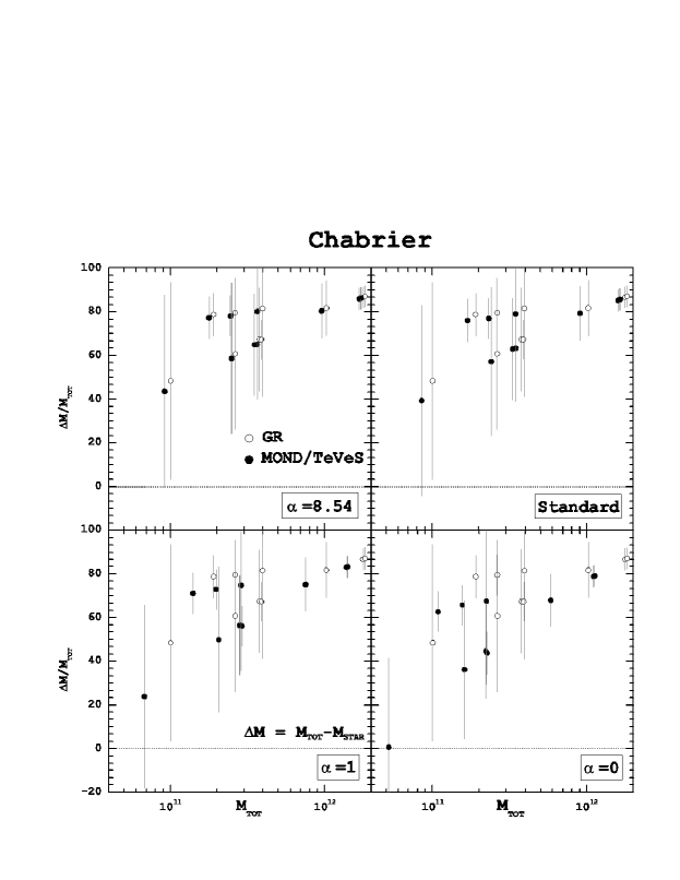
Figure 1: Plots of the aperture lensing mass of the systems versus the percentage discrepancy after comparison with the aperture stellar masses. The percentage difference between the stellar masses and the lensing masses are an indication of the dark matter required by the system. $M_{\rm TOT}$ is the lensing mass estimates within the aperture radius, $M_{\rm STAR}$ is the stellar mass estimate from fl11 . Plot for Chabrier stellar masses. GR represents the lensing mass when calculated using standard general relativity, and MOND when using the modified gravity.

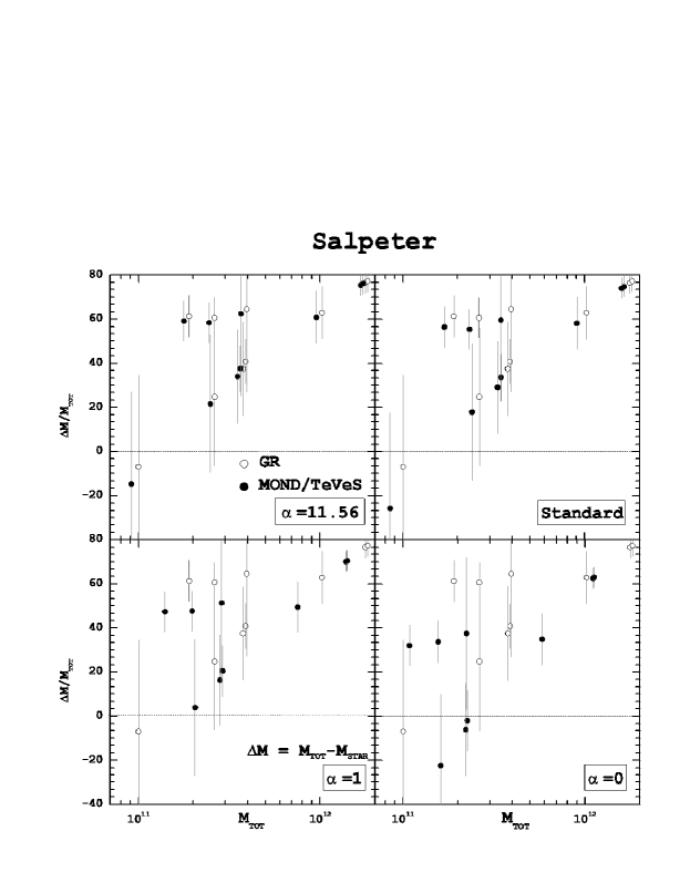
Figure 2: Plots of the aperture lensing mass of the systems versus the percentage discrepancy after comparison with the aperture stellar masses. The percentage difference between the stellar masses and the lensing masses are an indication of the dark matter required by the system. $M_{\rm TOT}$ is the lensing mass estimates within the aperture radius, $M_{\rm STAR}$ is the stellar mass estimate from fl11 . Plot for Salpeter stellar masses. GR represents the lensing mass when calculated using standard general relativity, and MOND when using the modified gravity.

Considering a Salpeter IMF (Fig. 2), the need for an additional component in all galaxies is reduced, as expected since the stellar mass estimates are greater than for a Chabrier IMF. Once again, the best case in favour of MOND/TeVeS with a single baryon component is $\alpha=0$, where three galaxies (BRI0952, B1152, HS0818) would not require any dark matter. However note that for a Salpeter IMF, both BRI0952 and B1152 are compatible with no dark matter within GR. Nevertheless, the data overall shows a significant need for dark matter, and the correlation between the lensing mass and “dark matter” excess remains valid with a Salpeter IMF. Furthermore, a consistent set of five lenses shows an excess higher than 50%. Note that the rejection of MOND/TeVeS in these systems is strongest when the best fit from rotation curves ($\alpha=11.56$) is chosen. Hence, it can be concluded that irrespective of the choice of IMF, neither MOND nor TeVeS can adequately account for the lensing observed using the luminous baryonic matter alone; an important result which confirms our previous conclusions fsy ; msy ; fmsy . In this paper, the extension of the analysis to larger apertures enables us to obtain an excess of lensing mass with greater confidence, as the outer regions are probed where it is thought that dark matter dominates.

The five robust lenses that pose a challenge are LBQS1009, HE1104, B1600, HE2149 and Q0957. The system Q0957 – the most massive one – is particularly interesting in this analysis. It consists of two independent image pairs, allowing its lensing mass to be calculated with two separate data sets. Not only are the lensing mass estimates from the different image pairs consistent, but this galaxy shows a particularly high dependence on dark matter. For the Chabrier case the dark matter dependence does not go below 77% (60% for the Salpeter case) even when the $\alpha=0$ parameterisation is considered. However, it is noted that Q0957 is a cD galaxy in the centre of a cluster q0957 , which means that an additional component clustering over larger scales, such as a 2 eV neutrino neutrinos , could accommodate the results. However, the other four galaxies (LBQS1009, HE1104, B1600, HE2149) are located in average density regions (either in the field or in small groups). Hence, for these systems the excess of lensing mass can only be reconciled if an additional, cold, component is added, i.e. CDM.

Regarding those lenses with a low (even negative!) excess of lensing matter, it is noted that one should be cautious when interpreting those data, as the error bars in the excess are very large, and always compatible with no excess. Averaging over a general sample of galaxies without taking care with the effects of such values can be misleading. Such averaging appears in Ref. chiu11 . In that work, when considering $\alpha=0$ (which is labeled as the “Bekenstein” parameterisation), the authors found that the average dark matter dependence for their sample was $-9.9\%$ using a Chabrier IMF. With the errors on the stellar masses, this result would be compatible with no dark matter. However, this average includes four galaxies with negative dark matter estimates (Q0142, BRI0952, Q1017 and SBS1520) which, according to their analysis, give dark matter contributions of $-85\%$, $-67\%$, $-64\%$ and $-47\%$, respectively. If the errors on the stellar masses are accounted for, these figures are reduced to $-15\%$, $-29\%$, $47\%$ and $11\%$, which means that only Q1017 and SBS1520 are at all compatible with positive dark matter estimates. Inclusion of these cases with a negative dark matter contribution, which is unphysical in a pressureless fluid baryon only scenario, will obviously skew the average. If one excludes these galaxies from the analysis, the average excess of lensing over stellar mass for the remaining sample is greater, $\approx 27\%$, which would be a great deal more difficult to account for without the addition of dark matter. For the Salpeter IMF case, so many of the galaxies are found to have a negative dark matter requirement that the average drops to $-40\%$. This clearly shows that cases with negative dark matter requirements need to be dealt with separately. For different parameterisations, a similar issue is found in this work. The “simple” case ($\alpha=1$) shows an average mass excess of $13\%$ for Chabrier and $-10\%$ for Salpeter. Removing the negative dark matter cases, this value increases to $42\%$ and $26\%$, both sufficiently high to question the validity of MOND/TeVeS. However, it is emphasized that an averaging approach is not a valid method to test the consistency of these theories; a case by case investigation offers the clearest insight into the dark matter requirement of lensing systems.

Furthermore, Ref. chiu11 does not take into account that the analysis of Ref. fmsy found a best fit parameter of the interpolating function from rotation curve data. Had the values of $\alpha=8.54$ for Chabrier and $\alpha=11.56$ for Salpeter IMFs been included, even with the averaging over negative mass estimates, a need for dark matter comparable to that in GR would have been found, a result which would, at the very least, soften their conclusions as regards the success of MOND.

V Conclusions

This paper extends previous analyses by the authors fsy ; msy ; fmsy using new lensing data, in order to perform tests of the MOND framework, as well as its fully relativistic generalisation TeVeS. The deflection angle equations were applied on a set of nine strong lensing systems from the CASTLES survey, to determine the lensing masses of those galaxies. The selection criteria by which galaxies were chosen was primarily dictated by our assumption of spherical symmetry. Only double lens systems and cases where our GR mass estimates were close to the standard mass estimates from Ref. fl11 – where neither spherical symmetry nor any particular mass profile was assumed – were included. The analysis of Ref. fl11 gives cumulative mass profiles out to a few effective radii. For some lenses, these calculations probe regions where the contribution from dark matter – in the standard framework of GR – dominates over the baryonic component. Hence, these data offer the opportunity to revisit and further develop our previous lensing work in both MOND and TeVeS and to draw firmer conclusions. It was found that, for a range of parameterisations of the MOND and TeVeS theories significant quantities of dark matter are present for at least five galaxies: LBQS1009, HE1104, B1600, HE2149 and Q0957, irrespective of the stellar initial mass function adopted. Furthermore, the choice of $\alpha=0$ – which gives the lowest contribution from dark matter – is a case that has been robustly ruled out by rotation curve data fmsy ; mu1 . Other parameterisations showed a even greater contribution for dark matter. In addition a trend is found whereby more massive galaxies present a higher excess with respect to the baryonic mass, a result that would be difficult to reconcile with a MOND/TeVeS approach.

Other options, such as a change of the cosmological parameters or variations in the values of the MOND/TeVeS constants have been shown to affect weakly the results msy . The most obvious recourse for proponents of MOND and TeVeS theories would be to find a more complex parameterisation of the gravitational interpolating function which would explain the excess lensing mass found in this sample, giving up one of the main advantages of such theories, namely the simpler description of astrophysical systems. It is found that some of these lenses robustly rule out the predictions of MOND and TeVeS assuming a single (baryonic) mass component over galaxy scales. Indeed if the claim to universality by theories such as MOND and TeVeS is to be taken seriously, then even a single robust case of a galaxy shown to require dark matter would be, though perhaps not fatal, a strong challenge for these theories. Although it is noted that Q0957 lives in a high density region – so that the lensing analysis may be probing scales larger than a typical galaxy halo – still an additional set of four robust candidates are found (LBQS1009, HE1104, B1600 and HE2149) that pose a serious challenge to these theories.

Thus, in sharp contrast with the conclusions of Ref. chiu11 which, as discussed above, had certain weaknesses in their analysis, our findings here support and extend our previous conclusions on the fate of MOND and at least the simplest of the TeVeS models. However, the future of modified theories of gravity does not end with MOND and TeVeS. In addition to multi-parametric interpolating functions, other modified theories of gravity such as Moffat’s MOdified Gravity (MOG) mog1 are in the early stages of being tested against lensing data mog3 and, at present, appear to offer a promising new arena of investigation. Moreover, it is possible that more complicated models, derived from microscopic theories of quantum gravity, such as strings and branes, incorporate some form of modification of gravity at low energies, which may mimick some but not all aspects of Modified Gravity Theories. An example of such a case is the D-particle Universe, discussed in sakellariadou , in which low-energy modifications of the gravitational laws do occur as a consequence of non trivial interactions of neutral matter with D-partricle space-time defects. Such modifications exist in the presence of significant components of Cold Dark Matter, e.g. supersymmetric partners, which in any case exist in low energy limits of (super)string theories. The use of gravitational lensing in testing such more complicated models is an interesting avenue to pursue, which would provide complementary information to other astrophysical, cosmological and collider tests of such theories.

References

- (1) See, e.g.: M. Tegmark et al. [SDSS Collaboration], Phys. Rev. D 74, 123507 (2006) [arXiv:astro-ph/0608632].
- (2) Y. Sofue, V. Rubin, Ann. Rev. Ast. Astrophys. 39, 137 (2001)
- (3) M. Milgrom, Astrophys. J. 270, 365 (1983).
- (4) J. D. Bekenstein, Phys. Rev. D 70, 083509 (2004) [Erratum-ibid. D 71, 069901 (2005)] [arXiv:astro-ph/0403694].
- (5) R. H. Sanders, Astrophys. J. 473, 117 (1996).
- (6) C. Skordis, D. F. Mota, P. G. Ferreira and C. Boehm, Phys. Rev. Lett. 96, 011301 (2006) [arXiv:astro-ph/0505519].
- (7) I. Ferreras, M. Sakellariadou and M. F. Yusaf, Phys. Rev. Lett., 100, 031302 (2008).
- (8) N.E. Mavromatos, M. Sakellariadou and M. F. Yusaf, Phys. Rev. D 79, 081301(R) (2009) [arXiv:0901.3932 [astro-ph.GA]].
- (9) I. Ferreras, N.E. Mavromatos, M. Sakellariadou and M. F. Yusaf Phys. Rev. D 80, 103506 (2009) [arXiv:0907.1463 [astro-ph.GA]].
- (10) http://cfa-www.harvard.edu/glensdata.
- (11) see e.g.: G. Gentile, H. S. Zhao and B. Famaey, arXiv:0712.1816 [astro-ph]; G. W. Angus, H. Shan, H. Zhao and B. Famaey, Astrophys. J. 654, L13 (2007) [arXiv:astro-ph/0609125]; R. H. Sanders, Mon. Not. Roy. Astron. Soc. 380, 331 (2007)
- (12) H. S. Zhao, D. J. Bacon, A. N. Taylor and K. Horne, Mon. Not. Roy. Astron. Soc. 368, 171 (2006) [arXiv:astro-ph/0509590].
- (13) M. -C. Chiu, C. -M. Ko, Y. Tian and H. Zhao, Phys. Rev. D 83 (2011) 063523 [arXiv:1008.3114 [astro-ph.GA]].
- (14) D. Leier, I. Ferreras, P. Saha and E. E. Falco, Astrophys. J. 740 (2011) 97 [arXiv:1102.3433 [astro-ph.GA]].
- (15) D. Giannios, Phys. Rev. D 71, 103511 (2005) [arXiv:gr-qc/0502122].
- (16) C. Skordis, Class. Quant. Grav. 26, 143001 (2009) [arXiv:0903.3602 [astro-ph.CO]].
- (17) S. Dodelson and M. Liguori, Phys. Rev. Lett. 97 (2006) 231301 [astro-ph/0608602].
- (18) C. R. Contaldi, T. Wiseman and B. Withers, Phys. Rev. D 78 (2008) 044034 [arXiv:0802.1215 [gr-qc]].
- (19) Bourliot et al, Phys. Rev. D 75, 063508 (2007)
- (20) E. Sagi and J. Bekenstein, Phys. Rev. D 77, 103512 (2008)
- (21) D. J. Mortlock and E. L. Turner, Mon. Not. Roy. Astron. Soc. 327 (2001) 557 [astro-ph/0106100].
- (22) M. Feix, C. Fedeli and M. Bartelmann, Astron. & Astrophysics 480, 313 (2008).
- (23) H. Zhao, B. Famaey, Astrophys. J. 638, L9 (2006).
- (24) B. Famaey and J. Binney, Mon. Not. Roy. Astron. Soc. 363, 603 (2005) [arXiv:astro-ph/0506723].
- (25) L. Hernquist, Astrophys. J. 356, 359 (1990).
- (26) P. G. Van Dokkum, C. Conroy, Nature, 468, 940 (2010)
- (27) M. Cappellari, et al., Nature, 484, 485 (2012)
- (28) E. E. Salpeter, Astrophys. J. 121, 161 (1955)
- (29) G. Chabrier, Publ. Astron. Soc. Pac. 115, 763 (2003) [arXiv:astro-ph/0304382].
- (30) I. Ferreras, P. Saha, S. Burles, Mon. Not. Roy. Astron. Soc. 383, 857 (2008)
- (31) I. Ferreras, P. Saha, D. Leier, F. Courbin, E. E. Falco Mon. Not. Roy. Astron. Soc. 409, L30 (2010)
- (32) I. Ferreras, P. Saha and L. L. R. Williams, Astrophys. J. 623, L5 (2005) [arXiv:astro-ph/0503168].
- (33) P. Young, J. E. Gunn, J. B. Oke, J. A. Westphal, J. Kristian, Astrophys. J. 241, 507 (1980)
- (34) J. W. Moffat, Journal of Cosmology and Astroparticle Physics 2006, 004 (2006), arXiv:gr-qc/0506021; J. W. Moffat, V. T. Toth, Class. Quant. Grav. 26, 085002 (2009), arXiv:0712.1796 [gr-qc].
- (35) J. W. Moffat, S. Rahvar V. T. Toth, 2012 arXiv:1204.2985 [astro-ph.CO]
- (36) N.E. Mavromatos and M. Sakellariadou, Phys. Lett. B 652, 97 (2007) [hep-th/0703156 [HEP-TH]]; J. R. Ellis, N. E. Mavromatos and M. Westmuckett, Phys. Rev. D 70, 044036 (2004) [gr-qc/0405066]; Phys. Rev. D 71, 106006 (2005) [gr-qc/0501060]; N. E. Mavromatos, V. A. Mitsou, S. Sarkar and A. Vergou, Eur. Phys. J. C 72, 1956 (2012) [arXiv:1012.4094 [hep-ph]].