Abstract

In this paper, we use the Poincare separation theorem for estimating the eigenvalues of the fine grid. We propose a randomized version of the algorithm where several different coarse grids are constructed thus leading to more comprehensive eigenvalue estimates. The proposed algorithm is suited for modern day multicore and distributed processing in the sense that no communication is required between the processors, however, at the cost of possible redundant computation.

1 Introduction

The problem of obtaining an approximation to eigenvalues and eigenvectors appears in several applications including data mining, chemical research, vibration analysis of mechanical structures, image processing etc. On the other hand, singular value decomposition has many useful applications in signal processing and statistics. For iterative methods, an estimate of extreme eigenvalue is useful for rapid Chebychev method [5] and in the construction of deflation preconditioners. An estimate of extreme eigenvalue leads to an estimate of condition number for symmetric positive matrix.

Poincare separation theorem [4] states that the eigenvalues of coarse grid matrix $P^{T}AP$ are “sandwiched” between the eigenvalues of the fine grid matrix $A$. In this paper, we consider samples of randomized coarsening scheme, i.e., the fine grid matrix is coarsened using special randomized interpolation operators $P$ leading to several samples of coarse grids preferably with different distribution of eigenvalues. We then compute the eigenvalues of these coarse grid matrices. When a sufficiently large number of coarse grids are taken then the smallest eigenvalue (singular value) of the fine grid is approximated by the smallest of the eigenvalues (singular values) of the coarse grid matrices and the largest eigenvalue (singular value) of the fine grid is approximated by the largest of the eigenvalues (singular values) of the coarse grid matrices. On the other hand, it is also possible to use the eigenvalues(singular values) of the coarse grid matrices as shifts for computing the eigenvalues(singular values) for the fine grid matrix.

The proposed algorithm is well suited for modern day multi-core and multiprocessor era since coarsening and subsequently the eigenvalue (singular value) of the resulting coarse grid could be computed independently without performing any inter node communication. The only communication required is when we gather the eigenvalues (singular values) computed by the processors. Given that communication often becomes more costly relative to computation it is essential to degisn algorithms that minimize communication as much as possible even at the cost of small redundant computation. This is the main reason behind the method proposed in this paper. However, we do not show any results for parallel case and here we only focus our study in understanding the quality of our approach.

The algorithms proposed has some similarity with the Jacobi-Davidson (JD) method [6] in the sense that both of these method try to approach the the eigenvalues of the fine grid via coarse grid, however, contrary to the sophisticated Jacobi-Davidson method, the method proposed is based on brute force approach, i.e., the method relies on creating enough coarse grid samples such that one of these coarse grid leads to the desired eigenvalue or singular value. Moreover, unlike JD method where the matrix P keeps growing by one column during the outer iteration in our method $P$ is fixed thus the coarse grid matrix $P^{T}AP$ is also fixed for each coarse grid sample.

This paper is organized as follows. In section (2), we review essential theorems and motivation behind the algorithms proposed. In section (3), we explain steps from clustering to obtaining the coarse matrix. All the algorithms for computing the eigenvalues and eigenvectors are presented in section (4), here we also show some the results of some numerical experiments and finally section (5) concludes this paper.

2 Poincaré separation theorem

Let $\lambda_{i}$ denote an arbitrary eigenvalue of $A$. The trace of an $n\times n$ matrix $A$ is defined to be the sum of the elements on the main diagonal of A, i.e.,

$$tr(A)=\sum_{i=1}^{n}a_{ii}$$

. If $f(x)=(x-\lambda_{1})^{d_{1}}\cdots(x-\lambda_{k})^{d_{k}}$ is the characteristic polynomial of a matrix $A$, then tr(A) is defined as follows

$$tr(A)=d_{1}\lambda_{1}+\cdots+d_{k}\lambda_{k}.$$

We have the following relation

$$\sum_{i=1}^{n}a_{ii}=\sum_{i=1}^{n}\lambda_{i}$$ (1)

Let $K^{T}$ denote the transpose of a matrix $K$ and let $I_{k}$ denote the identity matrix of size $k$. Here we will see how poincaré separates eigenvalues of two grids.

Theorem 1 (Poincaré).

Let $A$ be a symmetric $n\times n$ matrix with eigenvalues $\lambda_{1}\leq\lambda_{2}\leq\dots\leq\lambda_{n}$, and let $P$ be a semi-orthogonal $n\times k$ matrix with the property that $P^{T}P=I_{k}$. The eigenvalues $\mu_{1}\leq\mu_{2}\leq\cdots\leq\mu_{n-k+i}$ of $P^{T}AP$ are separated by the eigenvalues of $A$ as follows

$$\lambda_{i}\leq\mu_{i}\leq\lambda_{n-k+i}.$$ (2)

Proof.

The theorem is proved in [4]. ∎

In Figure (1), we show a part of the spectrum where eigenvalues of a coarse grid is distributed among the fine grid eigenvalues.

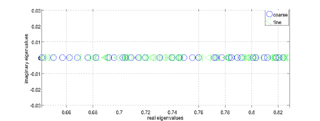
Figure 1: Poincare separates for sky 10$\times$10$\times$10 zoomed

Theorem 2.

If $A$ is a real symmetric $n\times n$ matrix with eigenvalues $\lambda_{1}\leq\lambda_{2}\leq\cdots\leq\lambda_{n}$, then the following holds

$$\min_{P^{T}P=I_{k}}tr(P^{T}AP) =\sum_{i=1}^{k}\lambda_{i},$$ (3)

$$\max_{P^{T}P=I_{k}}tr(P^{T}AP) =\sum_{i=1}^{k}\lambda_{n-k+i}.$$ (4)

Proof.

The theorem is proved in [4]. ∎

Theorem 3.

If $A$ is a real symmetric $n\times n$ matrix with eigenvalues $\lambda_{1}\leq\lambda_{2}\leq\cdots\leq\lambda_{n}$, and if the following conditions are satisfied

1. $tr(P^{T}AP)$ is minimum and

2. $P^{T}AP$ has simple eigenvalues

then we have

$$\mu_{i}=\lambda_{i},\quad 1\leq i\leq k,$$

where $\mu_{1}\leq\mu_{2}\leq\cdots\leq\mu_{k}$ are eigenvalues of $P^{T}AP$.

Proof.

Since $P^{T}AP$ has simple eigenvalues, we have $tr(P^{T}AP)=\sum_{i=1}^{k}\mu_{i}$. Also, from Theorem 2 above, we have

$$tr(P^{T}AP)=\sum_{i=1}^{k}\lambda_{i}.$$ (5)

We shall prove the hypothesis by contradiction. From 1, we have $\mu_{i}\geq\lambda_{i}$. Let there exist $j$, $1\leq j\leq k$, such that $\mu_{i}>\lambda_{i}$, then get

$$tr(P^{T}AP)=\sum_{i=1}^{k}\mu_{i}>\sum_{i=1}^{k}\lambda_{i}$$ (6)

contradicting (5). Thus, we must have $\mu_{i}=\lambda_{i}$. The proof is complete. ∎

The theorem above tells us that if we are able to find a matrix $P$ such that $tr(P^{T}AP)$ is minimum, then the first $k$ smallest eigenvalues of the matrix $A$ are simply the eigenvalues of the matrix $P^{T}AP$ provided $P^{T}AP$ has simple eigenvalues.

Theorem 4.

If $A$ is a real symmetric $n\times n$ matrix with eigenvalues $\lambda_{1}\leq\lambda_{2}\leq\cdots\leq\lambda_{n}$, and if the following conditions are satisfied

1. $tr(P^{T}AP)$ is maximum and

2. $P^{T}AP$ has simple eigenvalues

then we have

$$\mu_{i}=\lambda_{n-k+i},\quad 1\leq i\leq k,$$

where $\mu_{1}\leq\mu_{2}\leq\cdots\leq\mu_{k}$ are eigenvalues of $P^{T}AP$.

Proof.

Since $P^{T}AP$ has simple eigenvalues, we have $tr(P^{T}AP)=\sum_{i=1}^{k}\mu_{i}$. Also, from Theorem 2 above, we have

$$tr(P^{T}AP)=\sum_{i=1}^{k}\lambda_{n+i-k}.$$ (7)

We shall prove the hypothesis by contradiction. From 1, we have $\mu_{i}\leq\lambda_{i}$. Let there exist $j$, $1\leq j\leq k$, such that $\mu_{i}<\lambda_{i}$, then we get

$$tr(P^{T}AP)=\sum_{i=1}^{k}\mu_{i}<\sum_{i=1}^{k}\lambda_{i}$$ (8)

contradicting (7). Thus, we must have $\mu_{i}=\lambda_{i}$. The proof is complete. ∎

The theorem above tells us that if we are able to find a matrix $P$ such that $tr(P^{T}AP)$ is maximum, then the $k$ largest eigenvalues of the matrix $A$ are simply the eigenvalues of the matrix $P^{T}AP$ provided $P^{T}AP$ has simple eigenvalues. Determining first $k$ smallest or $k$ largest eigenvalues of a matrix is of prime importance in many applications.

Theorem 5 (Poincaré).

Let $A$ be a real $m\times n$ matrix with singular values

$$\sigma_{1}(A)\geq\sigma_{2}(A)\geq\dots$$

and let $U$ and $V$ be two matrices of order $m\times p$ and $n\times q$, respectively, such that $U^{*}U=I_{p}$ and $V^{*}V=I_{q}$. Let $B=U^{*}AV$ with singular values

$$\sigma_{1}(B)\geq\sigma_{2}(B)\geq\cdots$$

then the singular values of $B$ are separated by the singular values of $A$ as follows

$$\sigma_{i}(A)\geq\sigma_{i}(B)\geq\sigma_{i+r}(A),i=1,2,\cdots,min\{m,n\}$$

where $r=(m-p)+(n-q)$

Proof.

The theorem is proved in [4]. ∎

3 Clustering to coarsening

Our aim is to estimate the eigenvalues of the fine grid $A$ via the eigenvalues of coarse grid ($P^{T}AP$). Thus, the first step is clustering which then leads to the interpolation operator $P$ as follows. First a set of aggregates $G_{i}$ are defined. There are several different ways of doing aggregation (also described in [7]), some of them are as follows:

• This approach is closely related to the classical AMG [3] where one first defines the set of nodes $S_{i}$ to which $i$ is strongly negatively coupled, using the Strong/Weak coupling threshold $\beta$:

  $$S_{i}=\{\,j\neq i\mid a_{ij}<-\beta\ \text{max}|a_{ik}|\,\}.$$

  Then an unmarked node $i$ is chosen such that priority is given to the node with minimal $M_{i}$, here $M_{i}$ being the number of unmarked nodes that are strongly negatively coupled to $i$ [3].

• Several graph partitioning methods exists. Aggregation for AMG is created by calling a graph partitioner with number of aggregates as an input. The subgraph being partitioned are considered as aggregates. For instance, in this paper we use this approach by giving a call to the METIS graph partitioner routine METIS_PartGraphKway with the graph of the matrix and number of partitions as input parameters. The partitioning information is obtained in the output argument “part”. The part array maps a given node to its partition, i.e., part($i$) = $j$ means that the node $i$ is mapped to the $jth$ partition. In fact, the part array essentially determines the interpolation operator $P$. For instance, we observe that the ”part“ array is a discrete many to one map. Thus, the $i$th aggregate $G_{i}=\text{part}^{-1}(i)$, where

  $$\text{part}^{-1}(i)=\{\,j\in[1,\,N]\enspace\mid\enspace\text{part}(j)=i\,\}$$

• K-means clustering (see MATLAB): This clustering is defined in MATLAB and it produces random clustering i.e., a random “part” array defined above.

Let $J$ be the number of such aggregates, then the interpolation matrix $P$ is defined as follows

$$P_{ij}=\begin{cases}1,&\text{if $i\in G_{j}$,}\\ 0,&\text{otherwise,}\\ \end{cases}$$ (9)

Here, $1\leq i\leq N,\,1\leq j\leq J$, $N$ being the size of the original coefficient matrix $A$. Let $N=4$ be the size of $A$. Let there be two aggregates, $G_{1}=\{\,1,3\,\}$ and $G_{2}=\{\,2,4\,\}$, then the restriction operator $P^{T}$ is defined as follows $P^{T}=\left[\begin{array}[]{cccc}1&0&1&0\\ 0&1&0&1\end{array}\right]$. Further, we assume that the aggregates $G_{i}$ are such that

$$G_{i}\cap G_{j}=\phi,~{}\text{for}~{}i\neq j~{}\text{and}~{}\cup_{i}G_{i}=[1,N]$$ (10)

Here $[1,\,N]$ denotes the set of integers from $1$ to $N$. Notice that the matrix $P$ defined above is an $N\times J$ matrix but since it has only one non-zero entry (which are “one”) per row, the matrix can be defined by a single array containing the indices of the non-zero entries. The coarse grid matrix $A_{c}$ may be computed as follows

$$(A_{c})_{ij}=\sum_{k\in G_{i}}\sum_{l\in G_{j}}a_{kl}$$

where $1\leq i,\ j\leq N_{c}$, and $a_{kl}$ is the $(k,l)th$ entry of $A$.

4 Randomized coarsening and its applications

In this section, we list the algorithms that may lead to an approximation of eigenvalues or singular values. In algorithm (1), we show the steps for obtaining the eigenvalues of the input matrix $A$. Here, $\mu^{i}_{j}$ denotes the $jth$ eigenvalue of the $ith$ coarse grid. Later in the algorithm at step (7) $\mu^{i}_{j}$ is used as a shift to obtain the eigenvalue of the input matrix $A$. Since, Poincaré separation theorem tells us that $\mu^{i}_{j}$ will lie between two eigenvalues of the input matrix $A$, we expect it to converge to nearest one. However, it is possible that some other eigenvalue of other coarse grid also converges to the same eigenvalue and this redundant computation is inherent in this approach. In Algorithm (2), similar algorithm related to singular values is shown. Notice here that two interpolation matrices namely $U$ and $V$ are needed. The procedure for obtaining them is same as for $P$ except that we make use of two random clustering to construct the coarse grid matrix $U_{i}^{*}AV_{i}$. For clustering, we use of the “kmeans” clustering of MATLAB.

Algorithm 1 Eigenvalue estimate using multiple coarse grid

1:  INPUT: $A$, $J$, $k$

2:  OUTPUT: $\Lambda=$ eigenvalues of $A$

3:  for $i$ = 1 to $J$ do

4:     $A^{i}_{c}=P^{T}_{i}AP_{i}$

5:     Extract $\{\mu^{i}_{1},\mu^{i}_{2},\mu^{i}_{3},\dots\mu^{i}_{k}\}$ = eigenvalues($A^{i}_{c}$)

6:     for $j$ = 1 to $k$ do

7:        $\lambda^{i}_{j}$ = eigenvalues($A$, $\mu^{i}_{j}$) // $\mu^{i}_{j}$ is the shift

8:     end for

9:  end for

10:  $\Lambda=\{\lambda^{1}_{1},\lambda^{1}_{2},\lambda^{1}_{3},\dots,\lambda^{1}_{k}\}\cup\{\lambda^{2}_{1},\lambda^{2}_{2},\lambda^{2}_{3},\dots,\lambda^{2}_{k}\}\cup\dots\cup\{\lambda^{J}_{1},\lambda^{J}_{2},\lambda^{J}_{3},\dots,\lambda^{J}_{k}\}$

Algorithm 2 Singular value estimate using multiple coarse grid

1:  INPUT: $A$, $J$, $k$

2:  OUTPUT: $\Sigma=$singular value estimates of $A$

3:  for $i$ = 1 to $J$ do

4:     $A^{i}_{c}=U^{*}_{i}AV_{i}$

5:     Extract $\{\sigma^{i}_{1},\sigma^{i}_{2},\sigma^{i}_{3},\dots\sigma^{i}_{k}\}$ = eigenvalues($A^{i}_{c}$)

6:     for $j$ = 1 to $k$ do

7:        $\Sigma^{i}_{j}(A)$=singularvalue($A$, $\sigma^{i}_{j}$) // $\sigma^{i}_{j}$ is the shift

8:     end for

9:  end for

10:  $\Sigma=\{\Sigma^{1}_{1},\Sigma^{1}_{2},\Sigma^{1}_{3},\dots,\Sigma^{1}_{k}\}\cup\{\Sigma^{2}_{1},\Sigma^{2}_{2},\Sigma^{2}_{3},\dots,\Sigma^{2}_{k}\}\cup\dots\cup\{\Sigma^{J}_{1},\Sigma^{J}_{2},\Sigma^{J}_{3},\dots,\Sigma^{J}_{k}\}$

In Algorithm (3) and (4), we present special cases of the algorithms presented in Algorithms (1) and (2) to compute extreme eigenvalues and singular values respectively. We simply extract only the largest and smallest eigenvalues of all coarse grids. In Figure (2), we plot the singular values for rand(50) matrix available in MATLAB for 5 coarse grid samples. The coarse grid eigenvalues are then used as shift to determine the fine grid eigenvalues. In figure (3), we see in detail how the shifts converge to the actual eigenvalues.

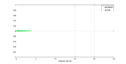
Figure 2: Poincaré separates for rand(50), $N_{c}=22$, J=5

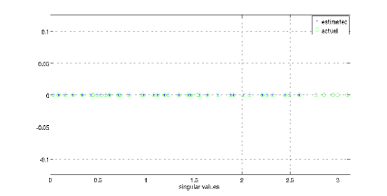
Figure 3: Poincaré separates for rand(50), $N_{c}=22$, J=5

Algorithm 3 Extreme eigenvalues using multiple coarse grid

1:  INPUT: $A$, $J$

2:  OUTPUT: $\{\Lambda_{max},\Lambda_{min}\}=$ approx. max and min eigenvalues of $A$

3:  for $i$ = 1 to $J$ do

4:     $A^{i}_{c}=P^{T}_{i}AP_{i}$ // perform coarsening

5:     $\mu^{i}_{max}$ = eigmax($A^{i}_{c}$) // just find the largest eigenvalue

6:     $\mu^{i}_{min}$ = eigmin($A^{i}_{c}$) // just find the smallest eigenvalue

7:  end for

8:  $\Lambda_{max}=max\{\mu^{1}_{max},\mu^{2}_{max},\mu^{3}_{max},\dots,\mu^{J}_{max}\}$

9:  $\Lambda_{min}=min\{\mu^{1}_{min},\mu^{2}_{min},\mu^{3}_{min},\dots,\mu^{J}_{min}\}$

Algorithm 4 Extreme singular values using multiple coarse grid

1:  INPUT: $A$, $J$

2:  OUTPUT: $\{\Sigma_{max},\Sigma_{min}\}=$ approx. max and min singular values of $A$

3:  for $i$ = 1 to $J$ do

4:     $A^{i}_{c}=U^{*}_{i}AV_{i}$ // perform coarsening

5:     $\sigma^{i}_{max}$ = singularmax($A^{i}_{c}$) // just find the largest singular value

6:     $\sigma^{i}_{min}$ = singularmin($A^{i}_{c}$) // just find the smallest singular value

7:  end for

8:  $\Sigma_{max}=max\{\sigma^{1}_{max},\sigma^{2}_{max},\sigma^{3}_{max},\dots,\sigma^{J}_{max}\}$

9:  $\Sigma_{min}=min\{\sigma^{1}_{min},\sigma^{2}_{min},\sigma^{3}_{min},\dots,\sigma^{J}_{min}\}$

References

• [1] G. Karypis, V. Kumar, A fast and high quality multilevel scheme for partitioning irregular graphs, SIAM J. Sci. Comp., (1999), 359-392.
• [2] R. E. Bellman, Introduction to matrix analysis, 2nd ed., New York: McGraw-Hill, p. 117, 1970
• [3] Y. Notay, An aggregation based algebraic multigrid, Num. Lin. Alg. Appl., vol 18, pp 539-564, 2011
• [4] C. R. Rao and M. B. Rao Matrix algebra and its applications to statistics and econometrics, World scientific publishing, 2004
• [5] Y. Saad, Iterative Methods for Sparse Linear Systems, PWS publishing company, Boston, MA, 1996.
• [6] G. L. G. Sleijpen and H. A. van der Vorst A Jacobi-Davidson iteration method for linear eigenvalue problems, SIAM J. Matrix Anal. Appl., vol 17, pp 401-425, 1996.
• [7] P. Kumar, Aggregation based on graph matching and inexact coarse grid solve for algebraic multigrid, arXiv:1105.3468v5, 2011