Engineering two-mode entangled states between two superconducting resonators by dissipation

Abstract

We present an experimental feasible scheme to synthesize two-mode continuous-variable entangled states of two superconducting resonators that are interconnected by two gap-tunable superconducting qubits. We show that, with each artificial atom suitably driven by a bichromatic microwave field to induce sidebands in the qubit-resonator coupling, the stationary state of the photon fields in the two resonators can be cooled and steered into a two-mode squeezed vacuum state via a dissipative quantum dynamical process, while the superconducting qubits remain in their ground states. In this scheme the qubit decay plays a positive role and can help drive the system to the target state, which thus converts a detrimental source of noise into a resource.

I introduction

Solid state devices based on superconducting circuits are promising candidates for studying fundamental physics and implementing quantum information protocols Zagoskin and Blais (2007); Clarke and K.Wilhelm (2008); Makhlin et al. (2001); Wendin and Shumeikoa (2007); You and Nori (2005). These devices, which can be designed and fabricated on demand, provide an unprecedented level of tunability and flexibility in the implementation of scalable quantum information processing. Three basic types of superconducting qubits, including chargeNakamura et al. (1999), fluxMooij et al. (1999) and phase qubitsYu et al. (2002), have been theoretically and experimentally investigated to realize quantum computation and communication. In general, these qubits are coupled either through circuit elements such as capacitances and inductances, or via a quantum bus Schoelkopf and Girvin (2008); Majer et al. (2007), a superconducting resonator. However, recent researches have shown that superconducting resonators can also be addressed and manipulated for quantum state generation Hofheinz et al. (2008); Wang et al. (2008); Zagoskin et al. (2008); Moon and Girvin (2005); Marquardt (2007); Rabl et al. (2004); Ojanen and Salo (2007); Li and Li (2011). Particularly, plenty of works have focused on the extension from single to more versatile multi-resonator architectures Mariantoni et al. (2008); Fisher et al. (2010); Li et al. (2009); Helmer et al. (2009), where the resonators are interconnected by superconducting qubits. These multi-resonator systems allow manipulation of spatially separated photon modes and engineering quantum states between physically distant cavities Mariantoni et al. (2011); Wang et al. (2011); Strauch et al. (2010); Hu and Tian (2011); Chen et al. (2009); Xue et al. (2007); Peng et al. (2012); Merkel and Wilhelm (2010); Semiao et al. (2009); Sun et al. (2006); Li et al. (2012); Yang et al. (2012, 2011).

In this work, we introduce an efficient scheme for the preparation of two-mode entangled states between two spatially separated superconducting resonators that are interconnected by two gap-tunable superconducting qubits. This proposal exploits a bichromatic microwave driving of each qubit to modify its coupling to the resonator modes, inducing sidebands in the qubit-resonator coupling Liu et al. (2007); Porras and Garcia-Ripoll (2012), and actively utilizes the qubit decay to drive the system to the desired state. We show that, combining the sidebands with the qubit decay, the stationary state of the photon fields in the two resonators can be steered into a two-mode squeezed vacuum state via a dissipative quantum dynamical process, while the superconducting qubits remain in their ground states. We detail the actual physical implementation of this scheme with the superconducting LC resonators inductively coupled to two gap-tunable $\alpha$-loop flux qubits. This work may open up promising perspectives for quantum information processing with coupled networks of superconducting resonators.

II The model

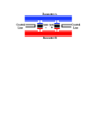
Figure 1: (Color online) The schematic for generating entanglement between two superconducting resonators. These resonators are interconnected by two gap-tunable superconducting qubits, which are independently controlled by external circuits.

We consider two gap-tunable superconducting qubits with ground state $|g\rangle$ and excited state $|e\rangle$, coupling to two superconducting resonators, as shown in Fig. 1. The energy levels of each qubit is individually driving by a bichromatic microwave field to induce sidebands in the qubit-cavity coupling. A typical gap-tunable superconducting qubit is the modified flux qubit where two junctions forms a superconducting quantum interference device (SQUID) to allow the modulation of the qubit gap Paauw et al. (2009). This modified flux qubit allows a fast change of the qubit resonance frequency while remaining at the degeneracy point. The free Hamiltonian describing the two qubits and the resonator modes is (let $\hbar=1$)

$$\hat{H}_{0}=\sum_{\lambda=1}^{2}(\frac{\delta}{2}\sigma_{z}^{\lambda}+\nu_{\lambda}\hat{a}_{\lambda}^{\dagger}\hat{a}_{\lambda}),$$ (1)

where $\delta$ is the qubit gap without external driving, $\sigma_{z}^{\lambda}$ is the Pauli operator, $\nu_{\lambda}$ is the resonator frequency, and $\hat{a}_{\lambda}^{\dagger}$ is the creation operator for the $\lambda$th resonator. The bare qubit-resonator interaction is given by

$$\hat{H}_{I}=\sum_{\lambda=1}^{2}\sum_{l=1}^{2}g_{l}^{(\lambda)}(\sigma_{+}^{\lambda}+\sigma_{-}^{\lambda})(\hat{a}_{l}^{\dagger}+\hat{a}_{l}),$$ (2)

where $g_{l}^{(\lambda)}$ is the coupling strength between the qubits and the resonators, and $\sigma_{\pm}^{j}$ the qubit ladder operators. We now consider a $\sigma_{z}$ driving with frequencies $\omega^{(\lambda)}_{d,l}$ for the $\lambda$th qubit Porras and Garcia-Ripoll (2012). For flux qubits, this driving can be implemented by an external magnetic field that induces a flux driving Paauw et al. (2009). Expressing the driving amplitude by the ratios $\xi_{l}^{(\lambda)}$ to the driving frequencies, we have

$$\hat{H}_{d}(t)=-\sum_{\lambda=1}^{2}\sum_{l=1}^{2}\xi_{l}^{(\lambda)}\omega^{(\lambda)}_{d,l}\cos(\omega^{(\lambda)}_{d,l}t)\sigma_{z}^{\lambda}.$$ (3)

In the following, the system-environment interaction is assumed Markovian, and then is described by a master equation in Lindblad form. Here we consider only relaxation and dephasing of the superconducting qubits, with the relaxation rate $\Gamma_{r}$ and dephasing rate $\Gamma_{\varphi}$. The time evolution of the density operator $\hat{\rho}$ for the whole system is then described by the master equation

$$\frac{d\hat{\rho}}{dt} = -i[\hat{H},\hat{\rho}]+\Gamma_{r}D[\sigma_{-}^{1}]\hat{\rho}+\Gamma_{r}D[\sigma_{-}^{2}]\hat{\rho}$$ (4)

$$+\Gamma_{\varphi}D[\sigma_{z}^{1}]\hat{\rho}+\Gamma_{\varphi}D[\sigma_{z}^{2}]\hat{\rho},$$

where $\hat{H}=\hat{H}_{0}+\hat{H}_{d}+\hat{H}_{I}$, and $D[A]\hat{\rho}=2A\hat{\rho}A^{\dagger}-A^{\dagger}A\hat{\rho}-\hat{\rho}A^{\dagger}A$.

We proceed to perform the unitary transformation $U_{1}(t)=e^{-i\hat{H}_{0}t}$, which leads to

$$\hat{H} = \sum_{\lambda=1}^{2}\sum_{l=1}^{2}g_{l}^{(\lambda)}(e^{i\delta t}\sigma_{+}^{\lambda}+e^{-i\delta t}\sigma_{-}^{\lambda})(e^{i\nu_{l}t}\hat{a}_{l}^{\dagger}+e^{-i\nu_{l}t}\hat{a}_{l})$$ (5)

$$-\sum_{\lambda=1}^{2}\sum_{l=1}^{2}\xi_{l}^{(\lambda)}\omega^{(\lambda)}_{d,l}\cos(\omega^{(\lambda)}_{d,l}t)\sigma_{z}^{\lambda}.$$

To engineer the desired qubit-photon coupling, we perform another unitary transformation

$$U_{2}(t) = Te^{-i\int_{0}^{t}\hat{H}_{d}(\tau)d\tau}$$ (6)

$$= 1-i\int_{0}^{t}\hat{H}_{d}(t_{1})dt_{1}$$

$$+(-i)^{2}\int_{0}^{t}dt_{1}\int_{0}^{t_{1}}dt_{2}\hat{H}_{d}(t_{1})\hat{H}_{d}(t_{2})+...$$

Keeping only the leading order in the rations $\xi_{l}^{(\lambda)}$, we have

$$\hat{H} = \sum_{\lambda=1}^{2}\sum_{j=1}^{2}\sigma_{+}^{\lambda}\{g_{j}^{(\lambda)}e^{i\delta t}(e^{i\nu_{j}t}\hat{a}_{j}^{\dagger}+e^{-i\nu_{j}t}\hat{a}_{j})$$ (7)

$$[1-\sum_{l=1}^{2}\xi_{l}^{(\lambda)}(e^{i\omega^{(\lambda)}_{d,l}t}-\text{h.c})]\}+\text{H.c.}$$

By setting $\omega^{(1)}_{d,1}=\delta-\nu_{1},\omega^{(1)}_{d,2}=\delta+\nu_{2}$, $\omega^{(2)}_{d,1}=\delta+\nu_{1},\omega^{(2)}_{d,2}=\delta-\nu_{2}$, and neglecting the fast oscillating terms under the rotating-wave approximation, we can get

$$\hat{H} = \sigma_{+}^{1}(g_{1}^{(1)}\xi_{1}^{(1)}\hat{a}_{1}+g_{2}^{(1)}\xi_{2}^{(1)}\hat{a}_{2}^{\dagger})+\sigma_{+}^{2}(g_{1}^{(2)}\xi_{1}^{(2)}\hat{a}_{1}^{\dagger}+g_{2}^{(2)}\xi_{2}^{(2)}\hat{a}_{2})$$ (8)

$$+\text{H.c.}$$

This Hamiltonian describes the red sideband ($\omega^{(1)}_{d,1}=\delta-\nu_{1}$) and blue sideband ($\omega^{(1)}_{d,2}=\delta+\nu_{2}$) excitations of the first qubit induced by the bichromatic microwave field with frequencies $\omega^{(1)}_{d,1}$ and $\omega^{(1)}_{d,2}$, and the blue sideband ($\omega^{(2)}_{d,1}=\delta+\nu_{1}$) and red sideband ($\omega^{(2)}_{d,2}=\delta-\nu_{2}$) excitations of the second qubit induced by another bichromatic microwave field with frequencies $\omega^{(2)}_{d,1}$ and $\omega^{(2)}_{d,2}$. The schematic diagram of these engineered qubit-photon couplings is shown in Fig. 2.

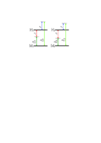
Figure 2: (Color online) The schematic of the engineered sideband couplings for the two superconducting qubits. The energy gap of the $j$th qubit oscillates at frequencies $\omega^{(j)}_{d,1}$ and $\omega^{(j)}_{d,2}$ induced by the flux driving of $\phi^{(j)}(t)(j=1,2)$.

We choose $g_{1}^{(1)}\xi_{1}^{(1)}=g_{2}^{(2)}\xi_{2}^{(2)}=\Theta_{1}$, $g_{2}^{(1)}\xi_{2}^{(1)}=g_{1}^{(2)}\xi_{1}^{(2)}=\Theta_{2}$, and $\Theta_{1}>\Theta_{2}$. In this case the Hamiltonian (8) can be rewritten as

$$\hat{H} = \sigma_{+}^{1}(\Theta_{1}\hat{a}_{1}+\Theta_{2}\hat{a}_{2}^{\dagger})+\sigma_{+}^{2}(\Theta_{1}\hat{a}_{2}+\Theta_{2}\hat{a}_{1}^{\dagger})+\text{H.c.}$$ (9)

We apply a unitary transformation $\tilde{\rho}=\hat{S}^{\dagger}(\zeta)\hat{\rho}\hat{S}(\zeta)$, where $\hat{S}(\zeta)=e^{\zeta\hat{a}_{1}\hat{a}_{2}-\zeta\hat{a}_{1}^{\dagger}\hat{a}_{2}^{\dagger}},\zeta=\tanh^{-1}\Theta_{2}/\Theta_{1}$. The master equation (4) for the system now becomes

$$\frac{d\tilde{\rho}}{dt} = -i[\tilde{H},\tilde{\rho}]+\Gamma_{r}D[\sigma_{-}^{1}]\tilde{\rho}+\Gamma_{r}D[\sigma_{-}^{2}]\tilde{\rho}$$ (10)

$$+\Gamma_{\varphi}D[\sigma_{z}^{1}]\tilde{\rho}+\Gamma_{\varphi}D[\sigma_{z}^{2}]\tilde{\rho},$$

where

$$\tilde{H} = \sqrt{\Theta^{2}_{1}-\Theta^{2}_{2}}(\hat{a}_{1}\sigma_{+}^{1}+\hat{a}_{2}\sigma_{+}^{2})+\text{H.c}.$$ (11)

The master equation (10) is equivalent to that of two independent Jaynes-Cummings models of two two-level atoms coupled to two cavity modes respectively, with atomic spontaneous emission and dephasing included. In the transformed picture, the $j$th superconducting qubit pulls the $j$th resonator mode into the vacuum state by a process in which the qubit continuously absorbs photons and decays back to its ground state. Therefore, the steady state of the system in the transformed picture is the vacuum $|00\rangle_{r}$ for the resonator modes $\hat{a}_{1},\hat{a}_{2}$, and $|g\rangle_{1}|g\rangle_{2}$ for the superconducting qubits. Reversing the unitary transformation, it can readily be seen that the state

$$|\psi_{S}\rangle = \hat{S}(\zeta)|00\rangle_{r}|g\rangle_{1}|g\rangle_{2}$$ (12)

is the unique stationary state of the master equation (4) i.e.,

$$\hat{\rho}(t\rightarrow\infty) = |\psi_{S}\rangle\langle\psi_{S}|.$$ (13)

The steady state (12) does not depend on the initial photon state of the resonators. Thus the resonators does not have to be initially cooled to the vacuum state in order to prepare such a state. Another distinct feature is that, in this scheme the qubit decay plays a positive role and can help drive the system to the target state, which thus converts a detrimental source of noise into a resource. This feature is particularly favorable for superconducting quantum circuits, since decoherence of the superconducting qubits is one of the generic sources of noise and sets the limits of quantum coherence in superconducting quantum circuits. The state $e^{\zeta\hat{a}_{1}\hat{a}_{2}-\zeta\hat{a}_{1}^{\dagger}\hat{a}_{2}^{\dagger}}|00\rangle_{r}$ is a two-mode squeezed state of the photon fields in the two resonators, which exhibits Einstein-Podolsky-Rosen (EPR) entanglement. The degree of squeezing (squeeze parameter $\zeta$) is determined by the ratio of $\Theta_{2}$ to $\Theta_{1}$, which can be controlled on demand through tuning the external experimental parameters.

To check the above model, we proceed to numerically solve the master equation including the decay of the resonator modes, i.e.,

$$\frac{d\hat{\rho}}{dt} = -i[\hat{H},\hat{\rho}]+\Gamma_{r}D[\sigma_{-}^{1}]\hat{\rho}+\Gamma_{r}D[\sigma_{-}^{2}]\hat{\rho}+\Gamma_{\varphi}D[\sigma_{z}^{1}]\hat{\rho}$$ (14)

$$+\Gamma_{\varphi}D[\sigma_{z}^{2}]\hat{\rho}+\kappa_{1}D[\hat{a}_{1}]\hat{\rho}+\kappa_{2}D[\hat{a}_{2}]\hat{\rho},$$

where $\kappa_{\lambda}$ is the photon loss rate for the $\lambda$th resonator. To quantify the validity of the proposal, we exploit the total variance $V=\langle(\Delta\hat{u})^{2}+(\Delta\hat{v})^{2}\rangle$ of a pair of EPR-like operators $\hat{u}=\hat{X}_{1}+\hat{X}_{2}$, and $\hat{v}=\hat{P}_{1}-\hat{P}_{2}$ , with $\hat{X}_{\lambda}=(\hat{a}_{\lambda}+\hat{a}^{\dagger}_{\lambda})/\sqrt{2}$, and $\hat{P}_{\lambda}=-i(\hat{a}_{\lambda}-\hat{a}^{\dagger}_{\lambda})/\sqrt{2},\lambda=1,2$. A two-mode Gaussian state is entangled if and only if $V<2$. For an ideal two-mode squeezed vacuum state, the total variance $V=\langle(\Delta\hat{u})^{2}+(\Delta\hat{v})^{2}\rangle=2e^{-2\zeta}$, implying this state exhibits EPR entanglement.

In Figure 3 we display the numerical results for time evolution of the total variance $V$ together with the results for an ideal two-mode squeezed vacuum state, under different values for the decay rates $\Gamma$, and $\kappa$, where $\Gamma_{r}\simeq\Gamma_{\varphi}\simeq\Gamma$, and $\kappa_{1}\simeq\kappa_{2}\simeq\kappa$ are assumed. The relevant parameters are chosen such that they are within the parameter range for which this scheme is valid and are accessible with present-day experimental setups. The initial state of the system is chosen as $\hat{\rho}(0)=|00\rangle_{r}|g\rangle_{1}|g\rangle_{2}$. From the simulation one can readily see that the model performs very well with the chosen parameters. At steady state ideal EPR entanglement ($\Theta_{2}/\Theta_{1}=0.75,V=0.286$) between the photon fields in the two resonators has been established if the resonator decay rate satisfies $\kappa<\{\Theta_{1},\Theta_{2},\Gamma\}$. However, when the resonator decay is comparable to or larger than $\Gamma$, the ideal EPR entanglement is spoiled by resonator decay. Therefore, implementing this proposal with high fidelity requires that $\kappa<\{\Theta_{1},\Theta_{2},\Gamma\}.$

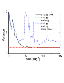
Figure 3: (Color online) Time evolution of the total variance $V$ through numerically solving the master equation (14), together with the result for an ideal two-mode squeezed vacuum state. The relevant parameters are chosen as $\xi_{1}^{(1)}\simeq\xi_{2}^{(2)}\simeq\xi_{1}=0.2,\xi_{2}^{(1)}\simeq\xi_{1}^{(2)}\simeq\xi_{2}=0.15,g_{1}^{(1)}\simeq g_{2}^{(1)}\simeq g_{1}^{(2)}\simeq g_{2}^{(2)}=g$.

III Two-mode entanglement between two superconducting LC resonators

In principle, the generic model can be implemented with various superconducting resonators coupled by two Josephson-junction-based superconducting qubits. Here we propose a convenient demonstration with two superconducting LC resonators inductively coupled to two gap-tunable flux qubits, as shown in Fig. 4.

The superconducting LC resonators made of a capacitor and an inductor are described by a simple harmonic oscillator Hamiltonian Johansson et al. (2006); Forn-Diaz et al. (2010) $\hat{H}_{r}=\sum_{\lambda=1}^{2}\nu_{\lambda}(\hat{a}_{\lambda}^{\dagger}\hat{a}_{\lambda}+1/2)$, where the resonance frequency $\nu_{\lambda}$ is determined by the respective capacitance $C_{\lambda}$ and the inductance $L_{\lambda}$: $\nu_{\lambda}=1/\sqrt{L_{\lambda}C_{\lambda}}$. For a micrometer scale LC resonator, the resonance frequency $\nu_{\lambda}$ is on the order of several GHzJohansson et al. (2006); Forn-Diaz et al. (2010). The quality factor $Q$ for a LC resonator can reach $Q\geq 10^{3}$, which leads to a decay rate for the resonator on the order of several MHz. These LC resonators are interconnected by two gap-tunable flux qubits which are inductively coupled to the resonators.

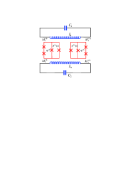
Figure 4: (Color online) The schematic of two superconducting LC resonators inductively coupled to the $\alpha$-loop flux qubits. The $\lambda$th flux qubit, controlled by the static magnetic flux $\Phi^{(\lambda)}$ and time-dependent flux driving $\phi^{(\lambda)}(t)$, is coupled to the $l$th resonator via mutual inductance $M^{(\lambda)}_{l}$.

We consider the so-called tunable-$\alpha$ flux qubits, as demonstrated in Ref. Paauw et al., 2009. Different from the flux qubit with three Josephson junctions, one of which has the coupling energy smaller than that of the other two junctions by a factor $\alpha$, here the small $\alpha$ junction is replaced by a so-called $\alpha$ loop, formed by a SQUID with two identical Josephson junctions. The $\lambda$th flux qubit can be operated at the degeneracy point with an external applied magnetic flux of $\Phi^{(\lambda)}\simeq\Phi_{0}/2$ and behaves effectively as a two-level system, where $\Phi_{0}=h/2e$ is the flux quantum. The qubit gap can be controlled via the flux driving $\phi^{(\lambda)}(t)$ through the SQUID loop, which can be implemented by the external microwave control lines. In this case, the Hamiltonian for the $\lambda$th flux qubit can be written as

$$\hat{H}_{q}^{(\lambda)}=-\frac{1}{2}\{\epsilon\sigma_{z}^{(\lambda)}+\Delta[\phi^{(\lambda)}(t)]\sigma_{x}^{(\lambda)}\}$$ (15)

in the basis of the persistent current states $\{|\circlearrowright\rangle,|\circlearrowleft\rangle\}$. Here $\epsilon=2I_{p}(\Phi^{(\lambda)}-\Phi_{0}/2)$, with $I_{p}$ is the persistent current in the qubit loop. The qubit gap $\Delta[\phi^{(\lambda)}(t)]$ depends on the flux driving, and can be separated into a static part $\delta$ and a time-dependent oscillating part $\propto\cos(\omega^{(\lambda)}_{d,l}t)$.

The two superconducting LC resonators couple to the flux qubits via the mutual inductance. The interaction between the $\lambda$th qubit and the $l$th LC resonator can be described by a coupling of dipolar nature in the basis of the persistent current states

$$\hat{H}^{(\lambda l)}_{I}=g^{(\lambda)}_{l}\sigma^{(\lambda)}_{z}(\hat{a}_{l}^{\dagger}+\hat{a}_{l}),$$ (16)

where the strength of the coupling is $g^{(\lambda)}_{l}=M^{(\lambda)}_{l}I_{p}\sqrt{\frac{\nu_{l}}{2L_{l}}}$, with $M^{(\lambda)}_{l}$ the mutual inductance between the $\lambda$th qubit and the $l$th LC resonator. In the basis of the eigenstates of the qubits, $\{|g\rangle,|e\rangle\}$, the total Hamiltonian reads

$$\hat{H} = \sum_{\lambda=1}^{2}[\frac{\omega_{q}}{2}\sigma_{z}^{\lambda}+\nu_{\lambda}\hat{a}_{\lambda}^{\dagger}\hat{a}_{\lambda}$$ (17)

$$+\sum_{l=1}^{2}g_{l}^{(\lambda)}(\cos\theta\sigma_{z}^{\lambda}-\sin\theta\sigma_{x}^{\lambda})(\hat{a}_{l}^{\dagger}+\hat{a}_{l})]$$

with $\omega_{q}=\sqrt{\epsilon^{2}+\Delta^{2}}$ and $\tan\theta=\Delta/\epsilon$. At the degeneracy point $\epsilon\simeq 0$, this leads to

$$\hat{H} = \sum_{\lambda=1}^{2}\{[\frac{\delta}{2}-\sum_{l=1}^{2}\xi_{l}^{(\lambda)}\omega^{(\lambda)}_{d,l}\cos(\omega^{(\lambda)}_{d,l}t)]\sigma_{z}^{\lambda}+\nu_{\lambda}\hat{a}_{\lambda}^{\dagger}\hat{a}_{\lambda}$$ (18)

$$+\sum_{l=1}^{2}g^{(\lambda)}_{l}(\sigma_{+}^{\lambda}+\sigma_{-}^{\lambda})(\hat{a}_{l}^{\dagger}+\hat{a}_{l})\}$$

From this Hamiltonian, one can engineer the desired photon-qubit couplings and prepare the photon fields in the two LC resonators into the two-mode squeezed vacuum state, via a dissipative quantum dynamical process following the reasoning in the above section.

We now discuss the relevant experimental parameters. Taking the capacitance and inductance of the LC resonators as 12 pF and 250 pH leads to $\nu_{1}\simeq\nu_{2}\simeq 2.9$ GHz Chiorescu et al. (2004). The mutual inductance $M^{(\lambda)}_{l}$ between the $\lambda$th flux qubit and the $l$th LC resonator can be about 20 pH Chiorescu et al. (2004). Thus we can obtain the coupling strength $g\simeq 200$ MHz. If we take $\xi_{1}=0.2,\xi_{2}=0.15$, then we obtain the effective coupling strength $\Theta_{1}\simeq 40$ MHz, and $\Theta_{2}\simeq 30$ MHz. The time for preparing the steady state (12) is determined by the decay rate $\Gamma$ of the flux qubit. Provided that $\sqrt{\Theta_{1}^{2}-\Theta_{2}^{2}}\geq\Gamma$, this time will be the order of a few times $1/\Gamma$. Moreover, if $\kappa\leq\Gamma$, the generated state will be nearly an ideal two-mode squeezed vacuum state. If we take $\Gamma\simeq 20$ MHz for the flux qubit, the preparing time will be about 250 ns.

IV conclusion

To conclude, we have presented an efficient scheme for the preparation of entangled states between two superconducting resonators that are interconnected by two gap-tunable superconducting qubits. We have shown that, with each qubit individually driven by a bichromatic microwave field to induce sidebands in the qubit-cavity coupling, the stationary state of the photon fields in the two resonators can be steered into a two-mode squeezed vacuum state via a dissipative quantum dynamical process. This proposal actively exploits the qubit decay to drive the system to the desired state and does not depend on the initial photon state of the resonators, which can be implemented with superconducting LC resonators inductively coupled to $\alpha$-loop flux qubits.

References

- Zagoskin and Blais (2007) A. Zagoskin and A. Blais, Physics in Canada 63, 215 (2007).
- Clarke and K.Wilhelm (2008) J. Clarke and F. K.Wilhelm, Nature (London) 453, 1031 (2008).
- Makhlin et al. (2001) Y. Makhlin, G. Schon, and A. Shnirman, Rev. Mod. Phys. 73, 357 (2001).
- Wendin and Shumeikoa (2007) G. Wendin and V. S. Shumeikoa, Low Temp. Phys. 33, 724 (2007).
- You and Nori (2005) J. Q. You and F. Nori, Phys. Today 58, 42 (2005).
- Nakamura et al. (1999) Y. Nakamura, Y. A. Pashkin, and J. S. Tsai, Nature (London) 398, 786 (1999).
- Mooij et al. (1999) J. E. Mooij, T. P. Orlando, L. Levitov, L. Tian, C. H. van der Wal, and S. Lloyd, Science 285, 1036 (1999).
- Yu et al. (2002) Y. Yu, S. Han, X. Chu, S. I. Chu, and Z. Wang, Science 296, 889 (2002).
- Schoelkopf and Girvin (2008) R. J. Schoelkopf and S. M. Girvin, Nature (London) 451, 664 (2008).
- Majer et al. (2007) J. Majer, J. M. Chow, J. M. Gambetta, J. Koch, B. R. Johnson, J. A. Schreier, L. Frunzio, D. I. Schuster, A. A. Houck, A. Wallraff, A. Blais, M. H. Devoret, S. M. Girvin, and R. J. Schoelkopf, Nature (London) 449, 443 (2007).
- Hofheinz et al. (2008) M. Hofheinz, E. M. Weig, M. Ansmann, R. C. Bialczak, E. Lucero, M. Neeley, A. D. OConnell, H. Wang, J. M. Martinis, and A. N. Cleland, Nature (London) 453, 310 (2008).
- Wang et al. (2008) H. Wang, M. Hofheinz, M. Ansmann, R. C. Bialczak, E. Lucero, M. Neeley, A. D. O’Connell, D. Sank, J. Wenner, A. N. Cleland, and J. M. Martinis, Phys. Rev. Lett. 101, 240401 (2008).
- Zagoskin et al. (2008) A. M. Zagoskin, E. Il’ichev, M. W. McCutcheon, J. F. Young, and F. Nori, Phys. Rev. Lett. 101, 253602 (2008).
- Moon and Girvin (2005) K. Moon and S. M. Girvin, Phys. Rev. Lett. 95, 140504 (2005).
- Marquardt (2007) F. Marquardt, Phys. Rev. B 76, 205416 (2007).
- Rabl et al. (2004) P. Rabl, A. Shnirman, and P. Zoller, Phys. Rev. B 70, 205304 (2004).
- Ojanen and Salo (2007) T. Ojanen and J. Salo, Phys. Rev. B 75, 184508 (2007).
- Li and Li (2011) P.-B. Li and F.-L. Li, Phys. Rev. A 83, 035807 (2011).
- Mariantoni et al. (2008) M. Mariantoni, F. Deppe, A. Marx, R. Gross, F. K. Wilhelm, and E. Solano, Phys. Rev. B 78, 104508 (2008).
- Fisher et al. (2010) R. Fisher, F. Helmer, S. J. Glaser, F. Marquardt, and T. Schulte-Herbruggen, Phys. Rev. B 81, 085328 (2010).
- Li et al. (2009) P.-B. Li, Y. Gu, Q.-H. Gong, and G.-C. Guo, Phys. Rev. A 79, 042339 (2009).
- Helmer et al. (2009) F. Helmer, M. Mariantoni, A. G. Fowler, J. von Delft, E. Solano, and F. Marquardt, Europhys. Lett. 85, 50007 (2009).
- Mariantoni et al. (2011) M. Mariantoni, H.Wang, R. C. Bialczak, M. Lenander, E. Lucero, M. Neeley, A. D. OConnell, D. Sank, M.Weides, J.Wenner, T. Yamamoto, Y. Yin, J. Zhao, J. M. Martinis, and A. N. Cleland, Nature Phys. 7, 287 (2011).
- Wang et al. (2011) H. Wang, M. Mariantoni, R. C. Bialczak, M. Lenander, E. Lucero, M. Neeley, A. D. O Connell, D. Sank, M. Weides, J. Wenner, T. Yamamoto, Y. Yin, J. Zhao, J. M. Martinis, and A. N. Cleland, Phys. Rev. Lett. 106, 060401 (2011).
- Strauch et al. (2010) F. W. Strauch, K. Jacobs, and R. W. Simmonds, Phys. Rev. Lett. 105, 050501 (2010).
- Hu and Tian (2011) Y. Hu and L. Tian, Phys. Rev. Lett. 106, 257002 (2011).
- Chen et al. (2009) M.-Y. Chen, M. W. Y. Tu, and W.-M. Zhang, Phys. Rev. B 80, 214538 (2009).
- Xue et al. (2007) F. Xue, Y. X. Liu, C. P. Sun, and F. Nori, Phys. Rev. B 76, 064305 (2007).
- Peng et al. (2012) Z. H. Peng, Y. X. Liu, Y. Nakamura, and J. S. Tsai, Phys. Rev. B 85, 024537 (2012).
- Merkel and Wilhelm (2010) S. T. Merkel and F. K. Wilhelm, New J. Phys. 12, 093036 (2010).
- Semiao et al. (2009) F. L. Semiao, K. Furuya, and G. J. Milburn, Phys. Rev. A 79, 063811 (2009).
- Sun et al. (2006) C. P. Sun, L. F. Wei, Y. X. Liu, and F. Nori, Phys. Rev. A 73, 022318 (2006).
- Li et al. (2012) P.-B. Li, S.-Y. Gao, and F.-L. Li, Phys. Rev. A 85, 014303 (2012).
- Yang et al. (2012) W. L. Yang, Z. Q. Yin, Q. Chen, C. Y. Chen, and M. Feng, Phys. Rev. A 85, 022324 (2012).
- Yang et al. (2011) W. L. Yang, Y. Hu, Z. Q. Yin, Z. J. Deng, and M. Feng, Phys. Rev. A 83, 022302 (2011).
- Liu et al. (2007) Y. X. Liu, L. F. Wei, J. R. Johansson, J. S. Tsai, and F. Nori, Phys. Rev. B 76, 144518 (2007).
- Porras and Garcia-Ripoll (2012) D. Porras and J. J. Garcia-Ripoll, Phys. Rev. Lett. 108, 043602 (2012).
- Paauw et al. (2009) F. G. Paauw, A. Fedorov, C. J. P. M. Harmans, and J. E. Mooij, Phys. Rev. Lett. 102, 090501 (2009).
- Johansson et al. (2006) J. Johansson, S. Saito, T. Meno, H. Nakano, M. Ueda, K. Semba, and H. Takayanagi, Phys. Rev. Lett. 96, 127006 (2006).
- Forn-Diaz et al. (2010) P. Forn-Diaz, J. Lisenfeld, D. Marcos, J. J. Garcia-Ripoll, E. Solano, C. J. P. M. Harmans, and J. E. Mooij, Phys. Rev. Lett. 105, 237001 (2010).
- Chiorescu et al. (2004) I. Chiorescu, P. Bertet, K. Semba, Y. Nakamura, C. J. P. M. Harmans, and J. E. Mooij, Nature (London) 431, 159 (2004).