Helicity–vorticity turbulent pumping of magnetic fields in the solar convection zone

Abstract

We study the effect of turbulent drift of a large-scale magnetic field that results from the interaction of helical convective motions and differential rotation in the solar convection zone. The principal direction of the drift corresponds to the direction of the large-scale vorticity vector. Thus, the effect produces a latitudinal transport of the large-scale magnetic field in the convective zone wherever the angular velocity has a strong radial gradient. The direction of the drift depends on the sign of helicity and it is defined by the Parker-Yoshimura rule. The analytic calculations are done within the framework of mean-field magnetohydrodynamics using the minimal $\tau$-approximation. We estimate the magnitude of the drift velocity and find that it can be several m/s near the base of the solar convection zone. The implications of this effect for the solar dynamo are illustrated on the basis of an axisymmetric mean-field dynamo model with a subsurface shear layer. We find that the helicity–vorticity pumping effect can have an influence on the features of the sunspot time–latitude diagram, producing a fast drift of the sunspot activity maximum at the rise phase of the cycle and a slow drift at the decay phase of the cycle.

1 Introduction

It is believed that the evolution of the large-scale magnetic field of the Sun is governed by the interplay between large-scale motions, like differential rotation and meridional circulation, turbulent convection flows and magnetic fields. One of the most important issues in solar dynamo theory is related to the origin of the equatorial drift of sunspot activity in the equatorial regions and, simultaneously at high latitudes, the poleward drift of the location of large-scale unipolar regions and quiet prominences. Parker (1955) and Yoshimura (1975) suggested that the evolution of large-scale magnetic activity of the Sun can be interpreted as dynamo waves propagating perpendicular to the direction of shear from the differential rotation. They found that the propagation can be considered as a diffusion process, which follows the iso-rotation surfaces of angular velocity in the solar convection zone. The direction of propagation can be modified by meridional circulation, anisotropic diffusion and the effects of turbulent pumping (see, e.g., Choudhuri et al., 1995; Kitchatinov, 2002; Guerrero and de Gouveia Dal Pino, 2008). The latter induces an effective drift of the large-scale magnetic field even though the mean flow of the turbulent medium may be zero.

The turbulent pumping effects can be equally important both for dynamos without meridional circulation and for the meridional circulation-dominated dynamo regimes. For the latter case the velocity of turbulent pumping has to be comparable to the meridional circulation speed. It is known that an effect of this magnitude can be produced by diamagnetic pumping and perhaps by so-called topological pumping. Both effects produce pumping in the radial direction and have not a direct impact on the latitudinal drift of the large-scale magnetic field.

Recently (Pipin, 2008; Mitra et al., 2009; Leprovost and Kim, 2010), it has been found that the helical convective motions and the helical turbulent magnetic fields interacting with large-scale magnetic fields and differential rotation can produce effective pumping in the direction of the large-scale vorticity vector. Thus, the effect produces a latitudinal transport of the large-scale magnetic field in the convective zone wherever the angular velocity has a strong radial gradient. It is believed that these regions, namely the tachocline beneath the solar convection zone and the subsurface shear layer, are important for the solar dynamo. Figure 1 illustrates the principal processes that induce the helicity–vorticity pumping effect. It is suggested that this effect produces an anisotropic drift of the large-scale magnetic field, which means that the different components of the large-scale magnetic field drift in different directions. Earlier work, e.g. by Kichatinov (1991) and Kleeorin and Rogachevskii (2003), suggests that the effect of anisotropy in the transport of mean-field is related to nonlinear effects of the global Coriolis force on the convection. Also, nonlinear effects of the large-scale magnetic field result in an anisotropy of turbulent pumping (Kleeorin et al., 1996). It is noteworthy, that the helicity–vorticity effect produces an anisotropy of the large-scale magnetic field drift already in the case of slow rotation and a weak magnetic field. A comprehensive study of the linear helicity–vorticity pumping effect for the case of weak shear and slow rotation was given by Rogachevskii et al. (2011) and their results were extended by DNS with a more general test-field method Brandenburg et al. (2012).

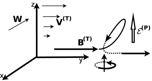
Figure 1: The field lines of the large-scale magnetic field, $\bm{B}^{(T)}$, are transformed by the helical motions to a twisted $\varOmega$-like shape. This loop is folded by the large-scale shear, $\bm{V}^{(T)}$, into the direction of the background large-scale magnetic field, $\bm{B}^{(T)}$. The induced electromotive force has a component, $\mbox{\boldmath${\cal E}$}{}^{(P)}$, which is perpendicular to the field $\bm{B}^{(T)}$. The resulting effect is identical to the effective drift of the large-scale magnetic field along the $x$-axis, in the direction opposite to the large-scale vorticity vector $\bm{W}=\nabla\times\bm{V}^{(T)}$, i.e., $\mbox{\boldmath${\cal E}$}{}^{(P)}\sim-\bm{W}\times\bm{B}^{(T)}$.

In this paper we analytically estimate the helicity–vorticity pumping effect taking into account the Coriolis force due to global rotation. The calculations were done within the framework of mean-field magnetohydrodynamics using the minimal $\tau$-approximation. The results are applied to mean field dynamo models, which are used to examine this effect on the dynamo. The paper is structured as follows. In the next section we briefly outline the basic equations and assumptions, and consider the results of calculations. Next, we apply the results to the solar dynamo. In Section 3 we summarize the main results of the paper. The details of analytical calculations are given in the Appendices A and B.

2 Basic equations

In the spirit of mean-field magnetohydrodynamics, we split the physical quantities of the turbulent conducting fluid into mean and fluctuating parts where the mean part is defined as an ensemble average. One assumes the validity of the Reynolds rules. The magnetic field $\bm{B}$ and the velocity $\bm{V}$ are decomposed as $\bm{B}=\overline{\bm{B}}+\bm{b}$ and $\bm{V}=\overline{\bm{V}}+\bm{u}$, respectively. Hereafter, we use small letters for the fluctuating parts and capital letters with an overbar for mean fields. Angle brackets are used for ensemble averages of products. We use the two-scale approximation (Roberts and Soward, 1975; Krause and Rädler, 1980) and assume that mean fields vary over much larger scales (both in time and in space) than fluctuating fields. The average effect of MHD-turbulence on the large-scale magnetic field (LSMF) evolution is described by the mean-electromotive force (MEMF), $\mbox{\boldmath${\cal E}$}{}=\left\langle\bm{u\times b}\right\rangle$. The governing equations for fluctuating magnetic field and velocity are written in a rotating coordinate system as follows:

$$\frac{\partial\bm{b}}{\partial t} = \nabla\times\left(\bm{u}\times\bm{\bar{B}}+\bm{\bar{V}}\times\bm{b}\right)+\eta\nabla^{2}\bm{b}+\mathfrak{G},$$ (1)

$$\frac{\partial u_{i}}{\partial t}+2\left(\bm{\varOmega}\times\bm{u}\right)_{i} = -\nabla_{i}\left(p+\frac{\left(\bm{b{\bm\cdot}\bar{B}}\right)}{\mu}\right)+\nu\Delta u_{i}$$

$$+ \frac{1}{\mu}\nabla_{j}\left(\bar{B}_{j}b_{i}+\bar{B}_{i}b_{j}\right)-\nabla_{j}\left(\bar{V}_{j}u_{i}+\bar{V}_{i}u_{j}\right)+f_{i}+\mathfrak{F}_{i},$$

where $\mathfrak{G},\mathfrak{F}$ stand for nonlinear contributions to the fluctuating fields, $p$ is the fluctuating pressure, $\bm{\varOmega}$ is the angular velocity responsible for the Coriolis force, $\bm{\bar{V}}$ is mean flow which is a weakly variable in space, and $\bm{f}$ is the random force driving the turbulence. Equations (1) and (2) are used to compute the mean-electromotive force $\mbox{\boldmath${\cal E}$}{}=\left\langle\bm{u\times b}\right\rangle$. It was computed with the help of the equations for the second moments of fluctuating velocity and magnetic fields using the double-scale Fourier transformation and the minimal $\tau$-approximations and for a given model of background turbulence. To simplify the estimation of nonlinear effects due to global rotation, we use scale-independent background turbulence spectra and correlation time. Details of the calculations are given in Appendix A. In what follows we discuss only those parts of the mean-electromotive force which are related to shear and the pumping effect.

2.1 Results

The large-scale shear flow is described by the tensor $\overline{V}_{i,j}=\nabla\overline{V}_{i}$. It can be decomposed into a sum of strain and vorticity tensors, $\nabla_{j}\overline{V}_{i}={\displaystyle\frac{1}{2}\left(\overline{V}_{i,j}+\overline{V}_{j,i}\right)-\frac{1}{2}\varepsilon_{ijp}\overline{W}_{p}}$, where $\overline{\bm{W}}=\boldsymbol{\nabla}\times\overline{\bm{V}}$ is the large-scale vorticity vector. The joint effect of large-scale shear, helical turbulent flows and magnetic fields can be expressed by the following contributions to the mean-electromotive force (omitting the $\alpha$-effect):

$$\mbox{\boldmath${\cal E}$}{}^{(H)} = \left(\bm{\overline{W}}\times\bm{\overline{B}}\right)\left(f_{2}^{(\gamma)}h_{\mathcal{C}}+f_{1}^{(\gamma)}h_{\mathcal{K}}\right)\tau_{c}^{2}+\bm{\tilde{V}}\left(\bm{B}\right)\left(f_{4}^{(\gamma)}h_{\mathcal{C}}+f_{3}^{(\gamma)}h_{\mathcal{K}}\right)\tau_{c}^{2}$$

$$+ \bm{e}\left[\left(\bm{e}\times\bm{\overline{W}}\right){\bm\cdot}\bm{\overline{B}}\right]\left(f_{6}^{(\gamma)}h_{\mathcal{C}}+f_{5}^{(\gamma)}h_{\mathcal{K}}\right)\tau_{c}^{2}+\left(\bm{e}\times\bm{\overline{W}}\right)\left(\bm{e}{\bm\cdot}\bm{\overline{B}}\right)\left(f_{8}^{(\gamma)}h_{\mathcal{C}}+f_{7}^{(\gamma)}h_{\mathcal{K}}\right)\tau_{c}^{2},$$

where $\bm{\tilde{V}}\left(\bm{B}\right)={\displaystyle\frac{\overline{B}_{j}}{2}\left(\overline{V}_{i,j}+\overline{V}_{j,i}\right)}$, ${\displaystyle\bm{e}=\frac{\boldsymbol{\varOmega}}{\left|\boldsymbol{\varOmega}\right|}}$ is the unit vector along the rotation axis, $\tau_{c}$ is the typical relaxation time of turbulent flows and magnetic fields, $h_{\mathcal{K}}^{\left(0\right)}=\left\langle\bm{u^{\left(0\right)}{\bm\cdot}\nabla\times u^{\left(0\right)}}\right\rangle$ and $h_{\mathcal{C}}^{\left(0\right)}={\displaystyle\frac{\left\langle\bm{b^{\left(0\right)}{\bm\cdot}\nabla\times b^{\left(0\right)}}\right\rangle}{\mu\rho}}$ are kinetic and current helicity of the background turbulence. These parameters are assumed to be known in advance. Functions $f_{n}^{(\gamma)}(\varOmega^{*})$ are given in Appendix B, they depend on the Coriolis number $\varOmega^{*}=2\varOmega_{0}\tau_{c}$ and describe the nonlinear effect due the Coriolis force, and $\varOmega_{0}$ is the global rotation rate.

For slow rotation, $\varOmega^{*}\ll 1$, we perform a Taylor expansion of $f_{n}^{(\gamma)}(\varOmega^{*})$ and obtain

$$\mbox{\boldmath${\cal E}$}{}^{(H)} = \frac{\tau_{c}^{2}}{2}\left(\bm{\overline{W}}\times\bm{\overline{B}}\right)\left(h_{\mathcal{C}}-h_{\mathcal{K}}\right)+\frac{\tau_{c}^{2}}{5}\bm{\tilde{V}}\left(\bm{B}\right)\left(3h_{\mathcal{K}}-\frac{13}{3}h_{\mathcal{C}}\right).$$ (4)

The coefficients in the kinetic part of Eq. (4) are two times larger than those found by Rogachevskii et al. (2011). This difference results from our assumption that the background turbulence spectra and the correlation time are scale-independent. The results for the magnetic part are in agreement with our earlier findings (see Pipin, 2008). The first term in Eq. (4) describes turbulent pumping with an effective velocity ${\displaystyle\frac{\tau_{c}^{2}\bm{\overline{W}}}{2}\left(h_{\mathcal{C}}-h_{\mathcal{K}}\right)}$ and the second term describes anisotropic turbulent pumping. Its structure depends on the geometry of the shear flow. For large Coriolis numbers, $\varOmega^{*}\gg 1$, only the kinetic helicity contributions survive:

$$\mbox{\boldmath${\cal E}$}{}^{(H)}=-\frac{\tau_{c}^{2}}{6}\left(\bm{\overline{W}}\times\bm{\overline{B}}\right)h_{\mathcal{K}}+\frac{\tau_{c}^{2}}{5}\bm{\tilde{V}}\left(\bm{B}\right)h_{\mathcal{K}}.$$ (5)

Figure 2 show the dependence of the pumping effects on the Coriolis number. We observe that for the terms $\left(\bm{\overline{W}}\times\bm{\overline{B}}\right)$ and $\bm{\tilde{V}}\left(\bm{B}\right)$ the effects of kinetic helicity are non-monotonic and have a maximum at $\varOmega^{*}\approx 1$. The effects of current helicity for these terms are monotonically quenched with increasing values of $\varOmega^{*}$. The additional contributions in Eq. (2.1) are rather small in comparison with the main terms. Thus, we can conclude that the first line in Eq. (2.1) describes the leading effect of pumping due to the helicity of turbulent flows and magnetic field. Below, we drop the contributions from the second line in Eq. (2.1) from our analysis.

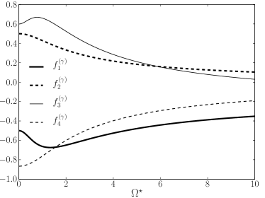
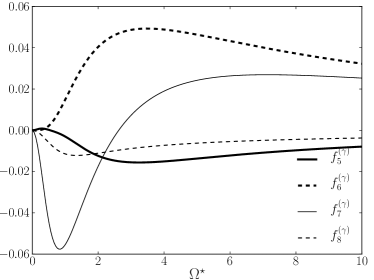
Figure 2: The dependence of the pumping effects on the Coriolis number. Solid lines show contributions from kinetic helicity and dashed lines the same for current helicity.

2.2 Helicity–vorticity pumping in the solar convection zone

2.2.1 The dynamo model

To estimate the impact of this pumping effect on the dynamo we consider the example of a dynamo model which takes into account contributions of the mean electromotive force given by Eq. (2.1). The dynamo model employed in this paper has been described in detail by Pipin and Kosovichev (2011a, c). This type of dynamo was proposed originally by Brandenburg (2005). The reader may find the discussion for different types of mean-field dynamos in Brandenburg and Subramanian (2005) and Tobias and Weiss (2007).

We study the standard mean-field induction equation in a perfectly conducting medium:

$$\frac{\partial\overline{\bm{B}}}{\partial t}=\boldsymbol{\nabla}\times\left(\mbox{\boldmath${\cal E}$}{}+\overline{\bm{U}}\times\overline{\bm{B}}\right),$$ (6)

where $\mbox{\boldmath${\cal E}$}{}=\overline{\bm{u\times b}}$ is the mean electromotive force, with $\bm{u,\,b}$ being fluctuating velocity and magnetic field, respectively, $\overline{\bm{U}}$ is the mean velocity (differential rotation and meridional circulation), and the axisymmetric magnetic field is:

$$\overline{\bm{B}}=\bm{e}_{\phi}B+\nabla\times\frac{A\bm{e}_{\phi}}{r\sin\theta},$$

where $\theta$ is the polar angle. The expression for the mean electromotive force ${\cal E}$ is given by Pipin (2008). It is expressed as follows:

$$\mathcal{E}_{i}=\left(\alpha_{ij}+\gamma_{ij}^{(\varLambda)}\right)\overline{B}-\eta_{ijk}\nabla_{j}\overline{B}_{k}+\mathcal{E}_{i}^{(H)}.$$ (7)

The new addition due to helicity and mean vorticity effects is marked by $\mbox{\boldmath${\cal E}$}{}^{H}$. The tensor $\alpha_{ij}$ represents the $\alpha$-effect. It includes hydrodynamic and magnetic helicity contributions,

$$\alpha_{ij} =C_{\alpha}\sin^{2}\theta\alpha_{ij}^{(H)}+\alpha_{ij}^{(M)},$$ (8)

$$\alpha_{ij}^{(H)} =\delta_{ij}\left\{3\eta_{T}\left(f_{10}^{(a)}\left(\bm{e}{\bm\cdot}\boldsymbol{\varLambda}^{(\rho)}\right)+f_{11}^{(a)}\left(\bm{e}{\bm\cdot}\boldsymbol{\varLambda}^{(u)}\right)\right)\right\}+$$ (9)

$$+e_{i}e_{j}\left\{3\eta_{T}\left(f_{5}^{(a)}\left(\bm{e}{\bm\cdot}\boldsymbol{\varLambda}^{(\rho)}\right)+f_{4}^{(a)}\left(\bm{e}{\bm\cdot}\boldsymbol{\varLambda}^{(u)}\right)\right)\right\}+$$ (10)

$$3\eta_{T}\left\{\left(e_{i}\varLambda_{j}^{(\rho)}+e_{j}\varLambda_{i}^{(\rho)}\right)f_{6}^{(a)}+\left(e_{i}\varLambda_{j}^{(u)}+e_{j}\varLambda_{i}^{(u)}\right)f_{8}^{(a)}\right\},$$ (11)

where the hydrodynamic part of the $\alpha$-effect is defined by $\alpha_{ij}^{(H)}$, $\bm{\boldsymbol{\varLambda}}^{(\rho)}=\boldsymbol{\nabla}\log\overline{\rho}$ quantifies the density stratification, $\bm{\boldsymbol{\varLambda}}^{(u)}=\boldsymbol{\nabla}\log\left(\eta_{T}^{(0)}\right)$ quantifies the turbulent diffusivity variation, and $\bm{e}=\boldsymbol{\varOmega}/\left|\varOmega\right|$ is a unit vector along the axis of rotation. The turbulent pumping, $\gamma_{ij}^{(\varLambda)}$, depends on mean density and turbulent diffusivity stratification, and on the Coriolis number $\varOmega^{*}=2\tau_{c}\varOmega_{0}$ where $\tau_{c}$ is the typical convective turnover time and $\varOmega_{0}$ is the global angular velocity. Following the results of Pipin (2008), $\gamma_{ij}^{(\varLambda)}$ is expressed as follows:

$$\gamma_{ij}^{(\varLambda)} =3\eta_{T}\left\{f_{3}^{(a)}\varLambda_{n}^{(\rho)}+f_{1}^{(a)}\left(\bm{e}{\bm\cdot}\boldsymbol{\varLambda}^{(\rho)}\right)e_{n}\right\}\varepsilon_{inj}-3\eta_{T}f_{1}^{(a)}e_{j}\varepsilon_{inm}e_{n}\varLambda_{m}^{(\rho)},$$ (12)

$$-3\eta_{T}\left(\varepsilon-1\right)\left\{f_{2}^{(a)}\varLambda_{n}^{(u)}+f_{1}^{(a)}\left(\bm{e}{\bm\cdot}\boldsymbol{\varLambda}^{(u)}\right)e_{n}\right\}\varepsilon_{inj}.$$ (13)

The effect of turbulent diffusivity, which is anisotropic due to the Coriolis force, is given by:

$$\eta_{ijk}=3\eta_{T}\left\{\left(2f_{1}^{(a)}-f_{2}^{(d)}\right)\varepsilon_{ijk}-2f_{1}^{(a)}e_{i}e_{n}\varepsilon_{njk}+\varepsilon C_{\omega}f_{4}^{(d)}e_{j}\delta_{ik}\right\}.$$ (14)

The last term in Eq. (14) describes Rädler’s $\boldsymbol{\varOmega}\times\bm{J}$ effect. The functions $f_{\{1-11\}}^{(a,d)}$ depend on the Coriolis number. They can be found in Pipin (2008); see also Pipin and Kosovichev (2011a) or Pipin and Sokoloff (2011)). In the model, the parameter $\varepsilon={\displaystyle\frac{\overline{\bm{b}^{2}}}{\mu_{0}\overline{\rho}\overline{\bm{u}^{2}}}}$, which measures the ratio between magnetic and kinetic energies of the fluctuations in the background turbulence, is assumed to be equal to 1. This corresponds to perfect energy equipartition. The $\varepsilon$ contribution in the second line of Eq. (12) describes the paramagnetic effect (Kleeorin and Rogachevskii, 2003). In the state of perfect energy equipartition the effect of diamagnetic pumping is compensated by the paramagnetic effect. We can, formally, skip the second line in Eq. (12) from our consideration if $\varepsilon=1$. To compare the magnitude of the helicity–vorticity pumping effect with the diamagnetic effect we will show results for the pumping velocity distribution with $\varepsilon=0$.

The contribution of small-scale magnetic helicity $\overline{\chi}=\overline{\bm{a{\bm\cdot}}\bm{b}}$ ($\bm{a}$ is the fluctuating vector-potential of the magnetic field) to the $\alpha$-effect is defined as

$$\alpha_{ij}^{(M)}=2f_{2}^{(a)}\delta_{ij}\frac{\overline{\chi}\tau_{c}}{\mu_{0}\overline{\rho}\ell^{2}}-2f_{1}^{(a)}e_{i}e_{j}\frac{\overline{\chi}\tau_{c}}{\mu_{0}\overline{\rho}\ell^{2}}.$$ (15)

The nonlinear feedback of the large-scale magnetic field to the $\alpha$-effect is described by a dynamical quenching due to the constraint of magnetic helicity conservation. The magnetic helicity, $\overline{\chi}$ , subject to a conservation law, is described by the following equation (Kleeorin and Rogachevskii, 1999; Subramanian and Brandenburg, 2004):

$$\frac{\partial\overline{\chi}}{\partial t} = -2\left(\mbox{\boldmath${\cal E}$}{}{\bm\cdot}\overline{\bm{B}}\right)-\frac{\overline{\chi}}{R_{\chi}\tau_{c}}+\boldsymbol{\nabla}{\bm\cdot}\left(\eta_{\chi}\boldsymbol{\nabla}\bar{\chi}\right),$$ (16)

where $\tau_{c}$ is a typical convective turnover time. The parameter $R_{\chi}$ controls the helicity dissipation rate without specifying the nature of the loss. The turnover time $\tau_{c}$ decreases from about 2 months at the bottom of the integration domain, which is located at $0.71R_{\odot}$, to several hours at the top boundary located at $0.99R_{\odot}$. It seems reasonable that the helicity dissipation is most efficient near the surface. The last term in Eq. (16) describes a turbulent diffusive flux of magnetic helicity (Mitra et al., 2010).

We use the solar convection zone model computed by Stix (2002), in which the mixing-length is defined as $\ell=\alpha_{\rm MLT}\left|\varLambda^{(p)}\right|^{-1}$, where $\bm{\boldsymbol{\varLambda}}^{(p)}=\boldsymbol{\nabla}\log\overline{p}\,$ quantifies the pressure variation, and $\alpha_{\rm MLT}=2$. The turbulent diffusivity is parameterized in the form, $\eta_{T}=C_{\eta}\eta_{T}^{(0)}$, where $\eta_{T}^{(0)}={\displaystyle\frac{u^{\prime}\ell}{3}}$ is the characteristic mixing-length turbulent diffusivity, $\ell$ is the typical correlation length of the turbulence, and $C_{\eta}$ is a constant to control the efficiency of large-scale magnetic field dragging by the turbulent flow. Currently, this parameter cannot be introduced in the mean-field theory in a consistent way. In this paper we use $C_{\eta}=0.05$. The differential rotation profile, $\varOmega=\varOmega_{0}f_{\varOmega}\left(x,\mu\right)$ (shown in Fig.3a) is a slightly modified version of the analytic approximation proposed by Antia et al. (1998):

$$f_{\varOmega}\left(x,\mu\right) = \frac{1}{\varOmega_{0}}\left[\varOmega_{0}+55\left(x-0.7\right)\phi\left(x,x_{0}\right)\phi\left(-x,-0.96\right)\right.$$

$$- \left.200\left(x-0.95\right)\phi\left(x,0.96\right)\right)$$

$$+ \left(21P_{3}\left(\mu\right)+3P_{5}\left(\mu\right)\right]\left(\frac{\mu^{2}}{j_{p}\left(x\right)}+\frac{1-\mu^{2}}{j_{e}\left(x\right)}\right)/\varOmega_{0},$$

$$j_{p} = \frac{1}{1+\exp\left(\frac{0.709-x}{0.02}\right)},\,\,j_{e}=\frac{1}{1+\exp\left(\frac{0.692-x}{0.01}\right)},$$

where $\varOmega_{0}=2.87\cdot 10^{-6}s^{-1}$ is the equatorial angular velocity of the Sun at the surface, $x=r/R_{\odot}$, $\phi\left(x,x_{0}\right)=0.5\left[1+\tanh\left[100(x-x_{0})\right]\right]$, and $x_{0}=0.71$.

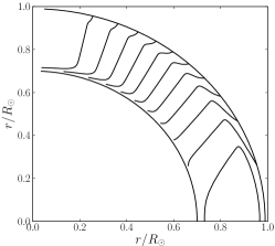
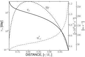
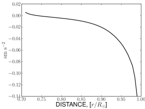
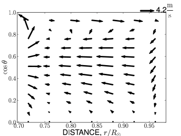
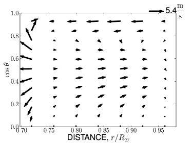
Figure 3: Distributions of the angular velocity and the turbulent parameters, and the kinetic helicity inside the solar convection zone. The bottom panel shows the patterns of the pumping velocity fields for the toroidal magnetic field(left) and for the poloidal field(right). They were computed on the basis of Eqs. (18,19,2.2.2).

2.2.2 Pumping effects in the solar convection zone

The components of the strain tensor $\bm{\tilde{V}}$ in a spherical coordinate system are given by the matrix:

$$\begin{array}[]{lll}\bm{\tilde{V}}&=&\left(\begin{array}[]{ccc}0&0&\tilde{V}_{\left(r,\varphi\right)}\\ 0&0&\tilde{V}_{\left(\theta,\varphi\right)}\\ \tilde{V}_{\left(r,\varphi\right)}&\tilde{V}_{\left(\theta,\varphi\right)}&0\end{array}\right)\end{array},$$

where we take into account only the azimuthal component of the large-scale flow, $\tilde{V}_{\left(r,\varphi\right)}=r\sin\theta\partial_{r}\varOmega\left(r,\theta\right)$,  $\tilde{V}_{\left(\theta,\varphi\right)}=\sin\theta\partial_{\theta}\varOmega\left(r,\theta\right)$, so $\bm{\hat{V}}\left(\bm{B}\right)=\left(B\tilde{V}_{\left(r,\varphi\right)},B\tilde{V}_{\left(\theta,\varphi\right)},\bm{B}_{i}^{p}\tilde{V}_{\left(i,\varphi\right)}\right)$. Substituting this into Eq. (2.1) we find the components of the mean-electromotive force for the helicity–vorticity pumping effect,

$$\mathcal{E}_{r}^{(H)} \!\!=\!\! \frac{\varOmega^{\ast}\tau_{c}}{2}\sin\theta\left\{\!\left[\!h_{\mathcal{K}}\left(f_{3}^{(\gamma)}-f_{1}^{(\gamma)}\right)+h_{\mathcal{C}}\left(f_{4}^{(\gamma)}-f_{2}^{(\gamma)}\right)\right]x\frac{\partial\tilde{\varOmega}}{\partial x}\!-\!2\left(\tilde{\varOmega}-1\right)\!\!\left[h_{\mathcal{K}}f_{1}^{(\gamma)}+h_{C}f_{2}^{(\gamma)}\right]\!\!\right\}\!\!B,$$ (18)

$$\mathcal{E}_{\theta}^{(H)} \!\!=\!\! \frac{\varOmega^{\ast}\tau_{c}}{2}\left\{\!\sin^{2}\theta\!\left[\!h_{\mathcal{K}}\left(f_{3}^{(\gamma)}-f_{1}^{(\gamma)}\right)\!+\!h_{\mathcal{C}}\left(f_{4}^{(\gamma)}-f_{2}^{(\gamma)}\right)\!\right]\!\!\frac{\partial\tilde{\varOmega}}{\partial\mu}-2\mu\left(\tilde{\varOmega}-1\right)\!\!\left[h_{\mathcal{K}}f_{1}^{(\gamma)}+h_{C}f_{2}^{(\gamma)}\right]\right\}\!\!B,$$ (19)

$$\mathcal{E}_{\phi}^{(H)} = -\frac{\varOmega^{\ast}\tau_{c}}{2}\frac{\sin\theta}{x}\left[h_{\mathcal{K}}\left(f_{3}^{(\gamma)}+f_{1}^{(\gamma)}\right)+h_{\mathcal{C}}\left(f_{4}^{(\gamma)}+f_{2}^{(\gamma)}\right)\right]\frac{\partial\left(\tilde{\varOmega},A\right)}{\partial\left(x,\mu\right)}$$

$$-\frac{\left(\tilde{\varOmega}-1\right)\varOmega^{\ast}\tau_{c}}{x\sin\theta}\left[h_{\mathcal{K}}f_{1}^{(\gamma)}+h_{C}f_{2}^{(\gamma)}\right]\left(\mu\frac{\partial A}{\partial x}+\frac{\sin^{2}\theta}{x}\frac{\partial A}{\partial\mu}\right),$$

where $h_{\mathcal{C}}=C_{\mathcal{C}}{\displaystyle\frac{\overline{\chi}}{\mu_{0}\overline{\rho}\ell^{2}}}$. It remains to define the kinetic helicity distribution. We use a formula proposed in our earlier study (see Kuzanyan et al. 2006),

$$h_{\mathcal{K}} ={\displaystyle C_{\eta}C_{\mathcal{K}}}\frac{\overline{u^{(0)2}}}{2}\frac{\partial}{\partial r}\log\left(\overline{\rho}\sqrt{\overline{u^{(0)2}}}\right)F_{1}\cos\theta,$$

where $F_{1}\left(\varOmega^{*}\right)$ was defined in the above cited paper. The radial profile of ${\displaystyle\frac{h_{\mathcal{K}}}{\cos\theta}}$ is shown in Figure 3. The radial profile of kinetic helicity is shown in Figure 3a of the above cited paper. The parameters $C_{\mathcal{K},\mathcal{C}}$ are introduced to switch on/off the pumping effects in the model.

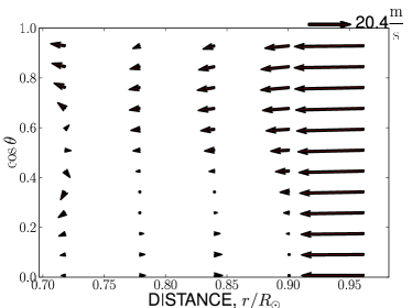
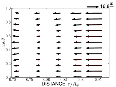
Figure 4: The patterns of the total (including the diamagnetic and the density gradient effects) pumping velocity fields for the toroidal magnetic field(left) and for the poloidal field(right).

The expressions given by Eq. (2.1) are valid for the case of weak shear, when $\tau_{c}\max\left(\left|\nabla_{i}\overline{V}_{j}\right|\right)\ll 1$. In terms of the strain tensor $\bm{\tilde{V}}$ this condition of weak shear implies ${\displaystyle\varOmega^{\star}}\max\left(\left|r\partial_{r}\tilde{\varOmega}\right|,\left|\partial_{\theta}\tilde{\varOmega}\right|\right)\ll 1$. This is not valid at the bottom of the solar convection zone where the radial gradient of the angular velocity is strong and $\varOmega^{\star}\gg 1$ and $\tau_{c}\max\left(\left|\nabla_{i}\overline{V}_{j}\right|\right)\approx 2$. Leprovost and Kim (2010) suggested that this pumping effect is quenched with increasing shear inversely proportional to $\left(\tau_{c}\max\left(\left|\nabla_{i}\overline{V}_{j}\right|\right)\right)^{1\dots 2}$. Therefore, we introduce an ad-hoc quenching function for the pumping effect:

$$f^{(S)}=\frac{1}{1+C_{S}{\displaystyle\varOmega^{*s}\left(\left|r\frac{\partial\tilde{\varOmega}}{\partial r}\right|+\left|\frac{\partial\tilde{\varOmega}}{\partial\theta}\right|\right)^{s}}},$$ (21)

where $C_{S}$ is a constant to control the magnitude of the quenching, and $s=1$. Results by Leprovost and Kim (2010) suggest $1<s<2$ in relation to geometry of the large-scale shear. We find that for the solar convection zone the amplitude of the pumping effect does not change very much ($\sim 1\,\mathrm{m/s}$) with $s$ varying in the range $1\dots 2$.

From the given relations, using $\mbox{\boldmath${\cal E}$}{}^{(H)}=\bm{U}^{\rm(eff)}\times\bm{\overline{B}}$, we find the effective drift velocity, $\bm{U}^{\rm(eff)}$, due to the helicity–vorticity pumping effect. Taking into account the variation of turbulence parameters in the solar convection zone we compute $\bm{U}^{\rm(eff)}$. The bottom panel of Figure 3 shows the distribution of the velocity field $\bm{U^{(eff)}}$ for the helicity–vorticity pumping effect for the toroidal and poloidal components of the large-scale magnetic field. The maximum velocity drift occurs in the middle and at the bottom of the convection zone. The direction of drift has equatorial and polar cells corresponding to two regions in the solar convection zone with different signs of the radial gradient of the angular velocity. The anisotropy in transport of the toroidal and poloidal components of the large-scale magnetic field is clearly seen.

The other important pumping effects are due to mean density and turbulence intensity gradients (Zeldovich, 1957; Kichatinov, 1991; Kichatinov and Rüdiger, 1992; Tobias et al., 2001). These effects were estimated using Eq. (12). For these calculations we put $C_{\eta}=1$, $\varepsilon=0$, $C_{\mathcal{K}}=1$ and $\overline{\chi}=0$. Figure 4 shows the sum of the pumping effects for the toroidal and poloidal components of mean magnetic fields including the helicity–vorticity pumping effect. In agreement with previous studies, it is found that the radial direction is the principal direction of mean-field transport in the solar convection zone. In its upper part the transport is downward because of pumping due to the density gradient (Kichatinov, 1991). At the bottom of the convection zone the diamagnetic pumping effect produces downward transport as well (Kichatinov, 1991; Rüdiger and Brandenburg, 1995). The diamagnetic pumping is quenched inversely proportional to the Coriolis number (e.g., Kichatinov, 1991; Pipin, 2008) and it has the same order of magnitude as the helicity–vorticity pumping effect. The latter effect modifies the direction of effective drift of the toroidal magnetic field near the bottom of the convection zone. There is also upward drift of the toroidal field at low latitudes in the middle of the convection zone. It results from the combined effects of density gradient and global rotation (Kichatinov, 1991; Krivodubskij, 2004). For the poloidal magnetic field the transport is downward everywhere in the convection zone. At the bottom of the convection zone the action of the diamagnetic pumping on the meridional component of the large-scale magnetic field is amplified due to the helicity–vorticity pumping effect.

The obtained pattern of large-scale magnetic field drift in the solar convection zone does not take into account nonlinear effects, e.g., because of magnetic buoyancy. The effect of mean-field buoyancy is rather small compared with flux-tube buoyancy (Kichatinov and Pipin, 1993, cf. Guerrero and Käpylä, 2011).

To find out the current helicity counterpart of the pumping effect we analyze dynamo models by solving Eqs. (6, 16). The governing parameters of the model are $C_{\eta}=0.05$, $C_{\omega}={\displaystyle\frac{1}{3}C_{\alpha}}$. We discuss the choice of the governing parameters later. The other parameters of the model are given in the Table 1. Because of the weakening factor $C_{\eta}$ the magnitude of the pumping velocity is about one order of magnitude smaller than what is shown in Figure 4.

Following Pipin and Kosovichev (2011b), we use a combination of “open” and “closed” boundary conditions at the top, controlled by a parameter $\delta=0.95$, with

$$\delta\frac{\eta_{T}}{r_{e}}B+\left(1-\delta\right)\mathcal{E}_{\theta}=0.$$ (22)

This is similar to the boundary condition discussed by Kitchatinov et al. (2000). For the poloidal field we apply a combination of the local condition $A=0$ and the requirement of a smooth transition from the internal poloidal field to the external potential (vacuum) field:

$$\delta\left(\left.\frac{\partial A}{\partial r}\right|_{r=r_{e}}-\left.\frac{\partial A^{(vac)}}{\partial r}\right|_{r=r_{e}}\right)+\left(1-\delta\right)A=0.$$ (23)

We assume perfect conductivity at the bottom boundary with standard boundary conditions. For the magnetic helicity, similar to Guerrero et al. (2010), we put $\boldsymbol{\nabla}_{r}\bar{\chi}=0$ at the bottom of the domain and $\bar{\chi}=0$ at the top of the convection zone.

Table 1: The parameters of the models. Here, $B_{\max}$ is the maximum of the toroidal magnetic field strength inside the convection zone, $P$ is the dynamo period of the model.

Model	$C_{\alpha}$	$R_{\chi}$	${\displaystyle C_{\mathcal{K}}}$	${\displaystyle C_{\mathcal{C}}}$	$B_{\max}$ [G]	$P$ [yr]
D1	0.025	$10^{3}$	0	0	500	16
D2	0.025	$10^{3}$	1	0	250	13
D3	0.03	$10^{3}$	1	10	300	13
D4	0.035	$5\cdot 10^{2}$	1	1	500	11

In this paper we study dynamo models which include Rädler’s $\boldsymbol{\varOmega}\times\bm{J}$ dynamo effect due to a large-scale current and global rotation (Rädler, 1969). There is also a dynamo effect due to large-scale shear and current (Rogachevskii and Kleeorin, 2003). The motivation to consider these addional turbulent sources in the mean-field dynamo comes from DNS dynamo experiments (Brandenburg and Käpylä, 2007; Käpylä et al., 2008; Hughes and Proctor, 2009; Käpylä et al., 2009) and from our earlier studies (Pipin and Seehafer, 2009; Seehafer and Pipin, 2009). The dynamo effect due to large-scale current gives an additional source of large-scale poloidal magnetic field. This can help to solve the issue with the dynamo period being otherwise too short. Also, in the models the large-scale current dynamo effect produces less overlapping cycles than dynamo models with $\alpha$-effect alone. The choice of parameters in the dynamo is justified by our previous studies (Pipin and Seehafer, 2009; Pipin and Kosovichev, 2011c), where we showed that solar-types dynamos can be obtained for $C_{\alpha}/C_{\omega}>2$. In those papers we find the approximate threshold to be $C_{\alpha}\approx 0.02$ for a given diffusivity dilution factor of $C_{\eta}=0.05$.

As follows from the results given in Fig.4, the kinetic helicity–vorticity pumping effect has a negligible contribution in the near-surface layers, where downward pumping due to density stratification dominates. Therefore, it is expected that the surface dynamo waves are not affected if we discard magnetic helicity from the dynamo equations. Figure 5 shows time-latitude diagrams for toroidal and radial magnetic fields at the surface and for toroidal magnetic field at the bottom of the convection zone for two dynamo models D1 and D2 with and without the helicity–vorticity pumping effect, but magnetic helicity is taken into account as the main dynamo quenching effect. To compare with observational data from a time-latitude diagram of sunspot area (e.g., Hathaway, 2011), we multiply the toroidal field component $B$ by factor $\sin\theta$. This gives a quantity, which is proportional to the flux of large-scale toroidal field at colatitude $\theta$. We further assume that the sunspot area is related to this flux.

Near the surface, models D1 and D2 give similar patterns of magnetic field evolution. At the bottom of the convection zone model D1 shows both poleward and equatorward branches of the dynamo wave propagation that is in agreement with the Parker-Yoshimura rule. Both branches have nearly the same time scale that equals $\simeq$16 years. The results from model D2 show that at the bottom of the convection zone the poleward branch of the dynamo wave dominates. Thus we conclude that the helicity–vorticity pumping effect alters the propagation of the dynamo wave near the bottom of the solar convection zone. We find that models with magnetic helicity contributions to the pumping effect do not change this conclusion.

a)

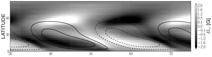
b)

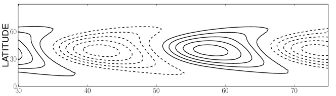
c)

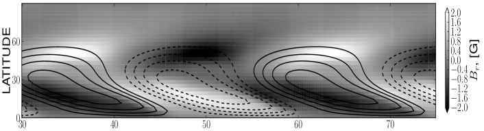
d)

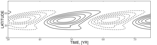
Figure 5: The time-latitude diagrams for the toroidal and radial magnetic fields for the models D1 and D2: a) the model D1, the toroidal field (iso-contours, $\pm.25KG$) near the surface and the radial field (gray-scale density plot); b) the model D1, the toroidal field at the bottom of the solar convection zone, the contours drawn in the range $\pm.5KG$; c) the same as for item a) for the model D2; d) the same as for item b) for the model D2.

Figure 6 shows a typical snapshot of the magnetic helicity distribution in the northern hemisphere for all our models. The helicity has a negative sign in the bulk of the solar convection zone. Regions with positive current helicity roughly correspond to domains of the negative large-scale current helicity concentration. They are located in the middle of the solar convection zone and at the high and low latitudes near the top of the solar convection zone. As follows from Fig. 6, the pumping effect due to current helicity may be efficient in the upper part of the solar convection zone where it might intensify the equatorial drift of the dynamo wave along iso-surfaces of the angular velocity.

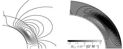
Figure 6: Snapshots for the mean magnetic field and the current helicity distributions at the north hemisphere in the model D4. Left panel shows the field lines of the poloidal component of the mean magnetic field. The right panel shows the toroidal magnetic field (iso-contours $\pm 500$G) and the current helicity (gray scale density plot).

We find that the pumping effect that results from magnetic helicity is rather small in our models. This may be due to the weakness of the magnetic field. Observations (Zhang et al., 2010) give about one order magnitude larger current helicity than what is shown in Fig. 6. In the model we estimate the current helicity as $H_{\mathcal{C}}={\displaystyle\frac{\overline{\chi}}{\mu_{0}\ell^{2}}}$. This result depends essentially on the mixing length parameter $\ell$. The stronger helicity is concentrated to the surface, the larger $H_{\mathcal{C}}$. In observations, we do not know from were the helical magnetic structures come from. In view of the given uncertainties we estimate the probable effect of a larger magnitude of magnetic helicity in the model by increasing the parameter $C_{\mathcal{C}}$ to 10 (model D3). In addition, we consider the results for the nonlinear model D4. It has a higher $C_{\alpha}$ and a lower $R_{\chi}$ to increase the nonlinear impact of the magnetic helicity on the large-scale magnetic field evolution.

The top panel of Figure 7 shows a time-latitude diagram of toroidal magnetic field and current helicity evolution near the surface for model D4. We find a positive sign of current helicity at the decay edges of the toroidal magnetic field butterfly diagram. There are also areas with positive magnetic helicity at high latitudes at the growing edges of the toroidal magnetic field butterfly diagram. The induced pumping velocity is about 1 $\mathrm{cm\,s^{-1}}$. The increase of the magnetic helicity pumping effect by a factor of 10 (model D3) shifts the latitude of the maximum of the toroidal magnetic field by about $5^{\circ}$ toward the equator. The induced pumping velocity is about 5 $\mathrm{cm\,s^{-1}}$.

Stronger nonlinearity (model D4) and a stronger magnetic helicity pumping effect (model D3) modify the butterfly diagram in different ways. Model D3 shows a simple shift of the maximum of toroidal magnetic field toward the equator. Model D4 shows a fast drift of large-scale toroidal field at the beginning of a cycle and a slow-down of the drift velocity as the cycle progresses.

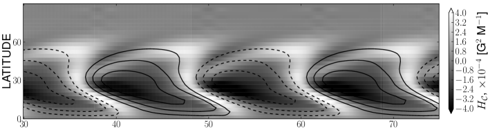
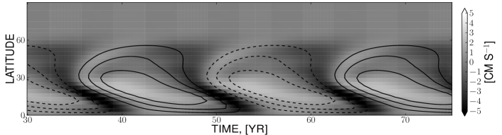
Figure 7: Top, the near-surface time-latitude diagrams for the toroidal magnetic field and the current helicity for the models D4. Bottom, the near-surface time-latitude diagrams for the toroidal magnetic field and the latitudinal component of the drift velocity induced by the magnetic helicity for the model D3.

Figure 8 shows in more detail the latitudinal drift of the maximum of the toroidal magnetic field evolution during the cycle (left panel in the Figure 8),

$$\lambda_{\max}(t)=90^{\circ}-\underset{\theta>45^{\circ}}{\max}\left(\left|B_{S}(\theta)\right|\sin\theta\right),$$ (24)

and the latitudinal drift of the centroid position of the toroidal magnetic field flux (cf. Hathaway, 2011)

$$\lambda_{C}(t)=90^{\circ}-\frac{\int_{0}^{\pi/2}\theta B_{S}(\theta)\sin\theta d\theta}{\int_{0}^{\pi/2}B_{S}(\theta)\sin\theta d\theta},$$ (25)

where $B_{S}(\theta)={\displaystyle\left\langle B\left(r,\theta\right)\right\rangle_{(0.9,0.99)R}}$ is the toroidal magnetic field, which is averaged over the surface layers. Note that the overlap between subsequent cycles influences the value of $\lambda_{C}$ more than the value of $\lambda_{\max}$. The behaviour of $\lambda_{\max}$ in models D1,D2 and D3 reproduces qualitatively the exponential drift of maximum latitude as suggested by Hathaway (2011):

$$\lambda_{C}(t)=28^{\circ}\exp\left(-\frac{12t}{90}\right),$$

where $t$ is time measured in years. Model D4 shows a change between fast (nearly steady dynamo wave) drift at the beginning of the cycle to slow drift at the decaying phase of the cycle. The overlap between subsequent cycles is growing from model D1 to model D4.

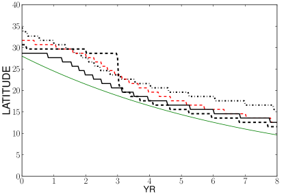
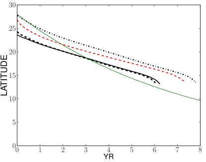
Figure 8: The drift of the latitude of maximum (left) and the centroid position of the magnetic flux at the near-surface layer in the models D(1-4). The dash-dotted line shows results for the model D1, the red dashed line - for the model D2, the solid black line - for the model D3, the black dashed line - for the model D4 and the solid green line shows the exponential law of the sunspot area centroid drift, as suggested by Hathaway (2011).

In all the models the highest latitude of the centroid position of the toroidal magnetic flux is below 30^∘. Models D3 and D4 have nearly equal starting latitude of the centroid position. It is about 24^∘. This means that a model with increased magnetic helicity pumping produces nearly the same effect for the shift of the centroid position as a model with a strong nonlinear effect of magnetic helicity.

3 Discussion and conclusions

We have shown that the interaction of helical convective motions and differential rotation in the solar convection zone produces a turbulent drift of large-scale magnetic field. The principal direction of the drift corresponds to the direction of the large-scale vorticity vector. The large-scale vorticity vector roughly follows to iso-surfaces of angular velocity. Since the direction of the drift depends on the sign of helicity, the pumping effect is governed by the Parker-Yoshimura rule (Parker, 1955; Yoshimura, 1975).

The effect is computed within the framework of mean-field magnetohydrodynamics using the minimal $\tau$-approximation. In the calculations, we have assumed that the turbulent kinetic and current helicities are given. The calculations were done for arbitrary Coriolis number. In agreement with Mitra et al. (2009) and Rogachevskii et al. (2011), the analytical calculations show that the leading effect of pumping is described by a large-scale magnetic drift in the direction of the large-scale vorticity vector and by anisotropic pumping which produces a drift of toroidal and poloidal components of the field in opposite directions. The component of the drift that is induced by global rotation and helicity (second line in Eq. (2.1)) is rather small compared to the main effect. The latter conclusion should be checked separately for a different model of background turbulence, taking into account the generation of kinetic helicity due to global rotation and stratification in a turbulent medium.

We have estimated the pumping effect for the solar convection zone and compared it with other turbulent pumping effects including diamagnetic pumping and turbulent pumping that results from magnetic fluctuations in stratified turbulence (Kichatinov, 1991; Pipin, 2008). The latter is sometimes referred to as “density-gradient pumping effect” (Krivodubskij, 2004). The diamagnetic pumping is upward in the upper part of the convection zone and downward near the bottom. The velocity field of density-gradient pumping is more complicated (see Figure 4). However, its major effect is concentrated near the surface. Both diamagnetic pumping and density-gradient pumping effects are quenched inversely proportional to the Coriolis number (Kichatinov, 1991; Pipin, 2008). The helicity–vorticity pumping effect modifies the direction of large-scale magnetic drift at the bottom of the convection zone. This effect was illustrated by a dynamo model that shows a dominant poleward branch of the dynamo wave at the bottom of the convection zone.

It is found that the magnetic helicity contribution of the pumping effect can be important for explaining the fine structure of the sunspot butterfly diagram. In particular, the magnetic helicity contribution results in a slow-down of equatorial propagation of the dynamo wave. The slow-down starts just before the maximum of the cycle. Observations indicate a similar behavior in sunspot activity (Ternullo, 2007; Hathaway, 2011). A behavior like this can be seen in flux-transport models as well (Rempel, 2006). For the time being it is unclear what are the differences between different dynamo models and how well do they reproduce the observations. A more detailed analysis is needed.

Appendix A

To compute ${\cal E}$ it is convenient to write equations (1) and (2) in Fourier space:

$$\left(\frac{\partial}{\partial t}+\eta z^{2}\right)\hat{b}_{j} = \frac{i}{\mu}z_{l}\hat{u}_{j}\left(\bm{z}\right)\bar{B}_{l}+$$

$$+ iz_{l}\int\left[\hat{b}_{l}(\bm{z-q)}\widehat{\bar{V}}_{j}(\bm{q})-\hat{b}_{j}\left(\bm{z-q)}\widehat{\bar{V}}_{l}(\bm{q})\right]d\bm{q}+\widehat{\mathfrak{G}}_{j}.\right.$$

$$\left(\frac{\partial}{\partial t}+\nu z^{2}\right)\hat{u}_{i} = \hat{f}_{i}+\widehat{\mathfrak{F}}_{i}-2\left(\bm{\varOmega}\widehat{\bm{z}}\right)\left(\widehat{\bm{z}}\times\widehat{\bm{u}}\right)_{i}$$

$$- i\pi_{if}(\bm{z)}z_{l}\int\left[\hat{u}_{l}(\bm{z-q)}\widehat{\bar{V}}_{f}(\bm{q})+\hat{u}_{f}\left(\bm{z-q)}\widehat{\bar{V}}_{l}(\bm{q})\right]{d}\bm{q}\right.$$

$$+ \frac{i}{\mu}\hat{b}_{i}\left(\bm{z}\right)\left(\bm{z}{\bm\cdot}\bar{\bm{B}}\right),$$

where the turbulent pressure was excluded from (2) by convolution with tensor $\pi_{ij}(\bm{z)}=\delta_{ij}-\hat{z}_{i}\hat{z}_{j}$, $\delta_{ij}$ is the Kronecker symbol and $\widehat{\bm{z}}$ is a unit wave vector. The equations for the second-order moments that make contributions to the mean-electro-motive force(MEMF) can be found directly from (Appendix A, Appendix A). As the preliminary step we write the equations for the second-order products of the fluctuating fields, and make the ensemble averaging of them,

$$\frac{\partial}{\partial t}\left\langle\hat{u}_{i}\left(\bm{z}\right)\hat{b}_{j}\left(\bm{z}^{\prime}\right)\right\rangle = i\,z^{\prime}_{l}\bar{B}_{l}\left\langle\hat{u}_{i}\left(\bm{z}\right)\hat{u}_{j}\left(\bm{\left.z^{\prime}\right)}\right\rangle\right.-2\left(\bm{\varOmega}\widehat{\bm{z}}\right)\varepsilon_{iln}\widehat{z_{l}}\left\langle\hat{u}_{n}(\bm{z})\hat{b}_{j}(\bm{z^{\prime}})\right\rangle$$

$$+ i\,z^{\prime}_{l}\int\left[\left\langle\hat{u}_{i}\left(\bm{z}\right)\hat{b}_{l}\left(\bm{z^{\prime}-q)}\right\rangle\widehat{\bar{V}}_{j}(\bm{q})-\left\langle\hat{u}_{i}\left(\bm{z}\right)\hat{b}_{j}\left(\bm{z^{\prime}-q)}\right\rangle\widehat{\bar{V}}_{l}(\bm{q})\right]d\bm{q}\right.\right.$$

$$- i\,\pi_{if}(\bm{z)}z_{l}\int\left[\left\langle\hat{u}_{l}\left(\bm{z-q)}\hat{b}_{j}\left(\bm{z}^{\prime}\right)\right\rangle\widehat{\bar{V}}_{f}(\bm{q})+\left\langle\hat{u}_{f}\left(\bm{z-q)}\hat{b}_{j}\left(\bm{z}^{\prime}\right)\right\rangle\widehat{\bar{V}}_{l}(\bm{q})\right]d\bm{q}\right.\right.$$

$$+ \frac{i}{\mu}\bar{B}_{l}z_{l}\langle\hat{b}_{i}\left(\bm{\left.z\right)}\hat{b}_{j}\left(\bm{z}^{\prime}\right)\rangle+Th_{ij}^{\varkappa}(\bm{z},\bm{z^{\prime}})-\left(\eta z^{\prime 2}+\nu z^{2}\right)\left\langle\hat{u}_{i}\left(\bm{z}\right)\hat{b}_{j}\left(\bm{z}^{\prime}\right)\right\rangle,\right.$$

$$\frac{\partial}{\partial t}\left\langle\hat{u}_{i}\left(\bm{z}\right)\hat{u}_{j}\left(\bm{z}^{\prime}\right)\right\rangle = -2\left(\bm{\varOmega}\widehat{\bm{z}}\right)\varepsilon_{iln}\widehat{z_{l}}\left\langle\hat{u}_{n}(\bm{z})\hat{u}_{j}(\bm{z^{\prime}})\right\rangle-2\left(\bm{\varOmega}\widehat{\bm{z}}^{\prime}\right)\varepsilon_{jln}\widehat{z_{l}^{\prime}}\left\langle\hat{u}_{i}(\bm{z})\hat{u}_{n}(\bm{z^{\prime}})\right\rangle$$

$$- i\,\pi_{if}(\bm{z)}z_{l}\int\left[\left\langle\hat{u}_{l}\left(\bm{z-q)}\hat{u}_{j}\left(\bm{z}^{\prime}\right)\right\rangle\widehat{\bar{V}}_{f}(\bm{q})+\left\langle\hat{u}_{f}\left(\bm{z-q)}\hat{u}_{j}\left(\bm{z}^{\prime}\right)\right\rangle\widehat{\bar{V}}_{l}(\bm{q})\right]d\bm{q}\right.\right.$$

$$- i\,\pi_{jf}(\bm{z^{\prime})}z^{\prime}_{l}\int\left[\left\langle\hat{u}_{i}\left(\bm{z}\right)\hat{u}_{l}\left(\bm{z-q)}\right\rangle\widehat{\bar{V}}_{f}(\bm{q})+\left\langle\hat{u}_{i}\left(\bm{z}\right)\hat{u}_{f}\left(\bm{z-q)}\right\rangle\widehat{\bar{V}}_{l}(\bm{q})\right]d\bm{q}\right.\right.$$

$$+ Th_{ij}^{v}(\bm{z},\bm{z^{\prime}})-\nu\left(z^{\prime 2}+z^{2}\right)\left\langle\hat{u}_{i}\left(\bm{z}\right)\hat{u}_{j}\left(\bm{z}^{\prime}\right)\right\rangle,$$

$$\frac{\partial}{\partial t}\left\langle\hat{b}_{i}\left(\bm{z}\right)\hat{b}_{j}\left(\bm{z}^{\prime}\right)\right\rangle = Th_{ij}^{h}(\bm{z},\bm{z^{\prime}})-\left(\eta z^{\prime 2}+\eta z^{2}\right)\left\langle\hat{b}_{i}\left(\bm{z}\right)\hat{b}_{j}\left(\bm{z}^{\prime}\right)\right\rangle$$

$$+ i\,z^{\prime}_{l}\int\left[\left\langle\hat{b}_{i}\left(\bm{z}\right)\hat{b}_{l}\left(\bm{z^{\prime}-q)}\right\rangle\widehat{\bar{V}}_{j}(\bm{q})-\left\langle\hat{b}_{i}\left(\bm{z}\right)\hat{b}_{j}\left(\bm{z^{\prime}-q)}\right\rangle\widehat{\bar{V}}_{l}(\bm{q})\right]d\bm{q},\right.\right.$$

where, the terms $Th_{ij}^{(\varkappa,v,h)}$ involve the third-order moments of fluctuating fields and second-order moments of them with the forcing term. Next, we apply the $\tau$-approximation, substituting the $Th_{ij}^{(\varkappa,v,h)}$-terms by the corresponding $\tau$ relaxation terms of the second-order contributions,

$$Th_{ij}^{(\varkappa)} \rightarrow-\left\langle\hat{m}_{i}\left(\bm{z}\right)\hat{b}_{j}\left(\bm{z}^{\prime}\right)\right\rangle/\tau_{c},$$ (31)

$$Th_{ij}^{(v)} \rightarrow-\frac{\left\langle\hat{m}_{i}\left(\bm{z}\right)\hat{m}_{j}\left(\bm{z}^{\prime}\right)\right\rangle-\left\langle\hat{m}_{i}\left(\bm{z}\right)\hat{m}_{j}\left(\bm{z}^{\prime}\right)\right\rangle^{\left(0\right)}}{\tau_{c}},$$ (32)

$$Th_{ij}^{(h)} \rightarrow-\frac{\left\langle\hat{b}_{i}\left(\bm{z}\right)\hat{b}_{j}\left(\bm{z}^{\prime}\right)\right\rangle-\left\langle\hat{b}_{i}\left(\bm{z}\right)\hat{b}_{j}\left(\bm{z}^{\prime}\right)\right\rangle^{(0)}}{\tau_{c}},$$ (33)

where the superscript $\dots{}^{\left(0\right)}$ denotes the moments of the background turbulence. Approximating these complicated contributions by the simple relaxation terms has to be considered as a questionable assumption. It involves additional assumptions (see Rädler and Rheinhardt, 2007), e.g., it is assumed that the second-order correlations in Eq. (8) do not vary significantly on the time scale of $\tau_{c}$. This assumption is consistent with scale separation between the mean and fluctuating quantities in the mean-field magneto hydrodynamics. The reader can find a comprehensive discussion of the $\tau$ -approximation in the above cited papers. Furthermore, we restrict ourselves to the high Reynolds numbers limit and discard the microscopic diffusion terms. The contributions of the mean magnetic field in the turbulent stresses will be neglected because they give the nonlinear terms in the cross helicity tensor. Also, $\tau_{c}$ is independent on $\bm{k}$ (cf, Rädler et al. 2003, Rogachevskii and Kleeorin 2003, Brandenburg and Subramanian 2005) and it is independent on the mean fields as well. This should be taken into account in considering the nonlinear effects due to rotation. Taking all the above assumptions into account, we get the system of equations for the moments for the stationary case:

$$\frac{\left\langle\hat{u}_{i}\left(\bm{z}\right)\hat{b}_{j}\left(\bm{z}^{\prime}\right)\right\rangle}{\tau_{c}} = -2\left(\bm{\varOmega}\widehat{\bm{z}}\right)\varepsilon_{iln}\widehat{z_{l}}\left\langle\hat{u}_{n}(\bm{z})\hat{b}_{j}(\bm{z^{\prime}})\right\rangle+i\,z^{\prime}_{l}\bar{B}_{l}\hat{u}_{i}\left(\bm{z}\right)\hat{u}_{j}\left(\bm{z^{\prime})}\right\rangle$$

$$+ i\,z^{\prime}_{l}\int\left[\left\langle\hat{u}_{i}\left(\bm{z}\right)\hat{b}_{l}\left(\bm{z^{\prime}-q)}\right\rangle\widehat{\bar{V}}_{j}(\bm{q})-\left\langle\hat{u}_{i}\left(\bm{z}\right)\hat{b}_{j}\left(\bm{z^{\prime}-q)}\right\rangle\widehat{\bar{V}}_{l}(\bm{q})\right]d\bm{q}\right.\right.$$

$$- i\,\pi_{if}(\bm{z)}z_{l}\int\left[\left\langle\hat{u}_{l}\left(\bm{z-q)}\hat{b}_{j}\left(\bm{z}^{\prime}\right)\right\rangle\widehat{\bar{V}}_{f}(\bm{q})+\left\langle\hat{u}_{f}\left(\bm{z-q)}\hat{b}_{j}\left(\bm{z}^{\prime}\right)\right\rangle\widehat{\bar{V}}_{l}(\bm{q})\right]d\bm{q}\right.\right.$$

$$+ \frac{i}{\mu}\bar{B}_{l}z_{l}\langle\hat{b}_{i}\left(\bm{\left.z\right)}\hat{b}_{j}\left(\bm{z}^{\prime}\right)\rangle,\right.$$

$$\frac{\left\langle\hat{m}_{i}\left(\bm{z}\right)\hat{m}_{j}\left(\bm{z}^{\prime}\right)\right\rangle}{\tau_{c}} = -2\left(\bm{\varOmega}\widehat{\bm{z}}\right)\varepsilon_{iln}\widehat{z_{l}}\left\langle\hat{u}_{n}(\bm{z})\hat{u}_{j}(\bm{z^{\prime}})\right\rangle-2\left(\bm{\varOmega}\widehat{\bm{z}}^{\prime}\right)\varepsilon_{jln}\widehat{z_{l}^{\prime}}\left\langle\hat{u}_{i}(\bm{z})\hat{u}_{n}(\bm{z^{\prime}})\right\rangle$$

$$- i\,\pi_{if}(\bm{z)}z_{l}\int\left[\left\langle\hat{u}_{l}\left(\bm{z-q)}\hat{u}_{j}\left(\bm{z}^{\prime}\right)\right\rangle\widehat{\bar{V}}_{f}(\bm{q})+\left\langle\hat{u}_{f}\left(\bm{z-q)}\hat{u}_{j}\left(\bm{z}^{\prime}\right)\right\rangle\widehat{\bar{V}}_{l}(\bm{q})\right]d\bm{q}\right.\right.$$

$$- i\,\pi_{jf}(\bm{z^{\prime})}z^{\prime}_{l}\int\left[\left\langle\hat{u}_{i}\left(\bm{z}\right)\hat{u}_{l}\left(\bm{z-q)}\right\rangle\widehat{\bar{V}}_{f}(\bm{q})+\left\langle\hat{u}_{i}\left(\bm{z}\right)\hat{u}_{f}\left(\bm{z-q)}\right\rangle\widehat{\bar{V}}_{l}(\bm{q})\right]d\bm{q}\right.\right.$$

$$+ \frac{\left\langle\hat{m}_{i}\left(\bm{z}\right)\hat{m}_{j}\left(\bm{z}^{\prime}\right)\right\rangle^{\left(0\right)}}{\tau_{c}}$$

$$\frac{\left\langle\hat{b}_{i}\left(\bm{z}\right)\hat{b}_{j}\left(\bm{z}^{\prime}\right)\right\rangle}{\tau_{c}} = \frac{\left\langle\hat{b}_{i}\left(\bm{z}\right)\hat{b}_{j}\left(\bm{z}^{\prime}\right)\right\rangle^{(0)}}{\tau_{c}}$$

$$+ i\,z^{\prime}_{l}\int\left[\left\langle\hat{b}_{i}\left(\bm{z}\right)\hat{b}_{l}\left(\bm{z^{\prime}-q)}\right\rangle\widehat{\bar{V}}_{j}(\bm{q})-\left\langle\hat{b}_{i}\left(\bm{z}\right)\hat{b}_{j}\left(\bm{z^{\prime}-q)}\right\rangle\widehat{\bar{V}}_{l}(\bm{q})\right]d\bm{q},\right.\right.$$

To proceed further, we have to introduce some conventions and notations that are widely used in the literature. The double Fourier transformation of an ensemble average of two fluctuating quantities, say $f$ and $g$, taken at equal times and at the different positions $\bm{x},\hskip 2.5pt\bm{x}^{\prime}$, is given by

$$\left\langle f\left(\bm{x}\right)g\left(\bm{x}^{\prime}\right)\right\rangle=\int\int\left\langle\hat{f}\left(\bm{z}\right)\hat{g}\left(\bm{z}^{\prime}\right)\right\rangle e^{i\,\left(\bm{z}{\bm\cdot}\bm{x}+\bm{z}^{\prime}{\bm\cdot}\bm{x}^{\prime}\right)}\mathrm{d}^{3}\bm{z}\mathrm{d}^{3}\bm{z}^{\prime}.$$ (37)

In the spirit of the general formalism of the two-scale approximation [Roberts and Soward, 1975] we introduce “fast” and “slow” variables. They are defined by the relative $\bm{r}=\bm{x}-\bm{x}^{\prime}$ and the mean $\bm{R}=\frac{1}{2}\left(\bm{x}+\bm{x}^{\prime}\right)$ coordinates, respectively. Then, Eq. (37) can be written in the form

$$\left\langle f\left(\bm{x}\right)g\left(\bm{x}^{\prime}\right)\right\rangle = \int\int\left\langle\hat{f}\left(\bm{k}+\frac{1}{2}\bm{K}\right)\hat{g}\left(-\bm{k}+\frac{1}{2}\bm{K}\right)\right\rangle\mathrm{e}^{i\,\left(\bm{K}{\bm\cdot}\bm{R}+\bm{k}{\bm\cdot}\bm{r}\right)}\mathrm{d}^{3}\bm{K}\mathrm{d}^{3}\bm{k},$$ (38)

where we have introduced the wave vectors $\bm{k}=\frac{1}{2}\left(\bm{z}-\bm{z}^{\prime}\right)$ and $\bm{K}=\bm{z}+\bm{z}^{\prime}$. Then, following to Subramanian and Brandenburg [2004], we define the correlation function of $\widehat{\bm{f}}$ and $\widehat{\bm{g}}$ obtained from (38) by integration with respect to $\bm{K}$,

$$\Phi\left(\hat{f},\hat{g},\bm{k},\bm{R}\right)=\int\left\langle\hat{f}\left(\bm{k}+\frac{1}{2}\bm{K}\right)\hat{g}\left(-\bm{k}+\frac{1}{2}\bm{K}\right)\right\rangle\mathrm{e}^{i\,\left(\bm{K}{\bm\cdot}\bm{R}\right)}\mathrm{d}^{3}\bm{K}.$$ (39)

For further convenience we define the second order correlations of momentum density, magnetic fluctuations and the cross-correlations of momentum and magnetic fluctuations via

$$\hat{v}_{ij}\left(\bm{k},\bm{R}\right) = \Phi(\hat{u}_{i},\hat{u}_{j},\bm{k},\bm{R}),\left\langle u^{2}\right\rangle\left(\bm{R}\right)=\int\hat{v}_{ii}\left(\bm{k},\bm{R}\right)\mathrm{d}^{3}\bm{k},$$ (40)

$$\hat{h}_{ij}\left(\bm{k},\bm{R}\right) = \Phi(\hat{b}_{i},\hat{b}_{j},\bm{k},\bm{R}),\left\langle b^{2}\right\rangle\left(\bm{R}\right)=\int\hat{h}_{ii}\left(\bm{k},\bm{R}\right)\mathrm{d}^{3}\bm{k},$$ (41)

$$\hat{\varkappa}_{ij}\left(\bm{k},\bm{R}\right) = \Phi(\hat{u}_{i},\hat{b}_{j},\bm{k},\bm{R}),\mathcal{E}_{i}\left(\bm{R}\right)=\varepsilon_{ijk}\int\hat{\varkappa}_{jk}\left(\bm{k},\bm{R}\right)\mathrm{d}^{3}\bm{k}.$$ (42)

We now return to equations (Appendix A), (Appendix A) and (Appendix A). As the first step, we solve these equations about $\boldsymbol{\varOmega}$ (non-linear effects of the Coriolis force) and make the Taylor expansion with respect to the “slow” variables and take the Fourier transformation, (39), about them. The details of this procedure can be found in [Subramanian and Brandenburg, 2004]. In result we get the following equations for the second moments

$$\frac{\hat{\varkappa}_{ij}}{\tau_{c}} = -\iota\mathcal{D}_{if}^{\left(0\right)}\left(\bm{B}{\bm\cdot}\bm{k}\right)\left(v_{fj}-\frac{m_{fj}}{\mu}\right)+\mathcal{D}_{if}^{\left(0\right)}\bar{V}_{j,l}\hat{\varkappa}_{fl}-\mathcal{D}_{if}^{\left(0\right)}\bar{V}_{f,l}\hat{\varkappa}_{lj}+$$

$$+ 2\mathcal{D}_{ip}^{\left(0\right)}\hat{k}_{p}\hat{k}_{f}\hat{\varkappa}_{lj}\bar{V}_{f,l}+\mathcal{D}_{if}^{\left(0\right)}k_{l}\bar{V}_{f,l}\frac{\partial\hat{\varkappa}_{fj}}{\partial k_{f}},$$

$$\mathcal{D}_{if}^{\left(0\right)} = \frac{\delta_{if}+\psi_{\varOmega}\hat{k}_{p}\varepsilon_{ifp}+\psi_{\varOmega}^{2}\hat{k}_{i}\hat{k}_{f}}{1+\psi_{\varOmega}^{2}},\,\psi_{\varOmega}=2\left(\bm{\boldsymbol{\varOmega}{\bm\cdot}}\hat{\bm{k}}\right)\tau_{c}$$

$$\frac{\hat{v}_{ij}}{\tau_{c}} = T_{ijnm}^{(0)}\left(\frac{\hat{v}_{nm}^{(0)}}{\tau_{c}}+2\hat{k}_{f}\bar{V}_{f,l}\left(\hat{k}_{n}\hat{v}_{lm}+\hat{k}_{m}\hat{v}_{nl}\right)-\bar{V}_{n,l}\hat{v}_{lm}-\bar{V}_{m,l}\hat{v}_{nl}+k_{l}\bar{V}_{f,l}\frac{\partial\hat{v}_{nm}}{\partial k_{f}}\right),$$ (44)

$$T_{ijnm}^{\left(0\right)} = \delta_{in}\delta_{jm}+\frac{\psi_{\varOmega}\hat{k}_{p}}{M}\left(\varepsilon_{inp}\delta_{jm}+\varepsilon_{jmp}\delta_{in}\right)$$

$$- \frac{\psi_{\varOmega}^{2}}{M}\left(\delta_{ij}\pi_{nm}-\delta_{nm}\hat{k}_{i}\hat{k}_{j}+\delta_{im}\hat{k}_{n}\hat{k}_{j}+\delta_{nj}\hat{k}_{i}\hat{k}_{m}-2\delta_{n\left[i\right.}\delta_{\left.j\right]m}\right),$$

$$M = 1+4\psi_{\varOmega}^{2}$$

$$\hat{h}_{ij} = \hat{h}_{ij}^{\left(0\right)}+\tau_{c}\hat{h}_{il}\bar{V}_{j,l}+\tau_{c}\hat{h}_{lj}\bar{V}_{i,l}+\tau_{c}k_{l}\bar{V}_{f,l}\frac{\partial\hat{h}_{ij}}{\partial k_{f}}$$ (45)

These equations were solved with respect to the shear tensor, $\overline{V}_{i,j}=\nabla_{j}\overline{V}_{i}$, by means of perturbation procedure. One remains to define the spectra of the background turbulence. We will adopt the isotropic form of the spectra [Roberts and Soward, 1975]. Additionally, the background magnetic fluctuations are helical while there is no prescribed kinetic helicity in the background turbulence:

$$\hat{v}_{ij}^{(0)} = \left\{\pi_{ij}\left(\bm{k}\right)\frac{E\left(k,\bm{R}\right)}{8\pi k^{2}}-i\,\varepsilon_{ijp}k_{p}\frac{\mathcal{H}\left(k,\bm{R}\right)}{8\pi k^{4}}\right\},$$ (46)

$$\hat{h}_{ij}^{(0)} = \left\{\pi_{ij}\left(\bm{k}\right)\frac{\mathcal{B}\left(k,\bm{R}\right)}{8\pi k^{2}}-i\,\varepsilon_{ijp}k_{p}\frac{\mathcal{N}\left(k,\bm{R}\right)}{8\pi k^{4}}\right\},$$ (47)

where, the spectral functions $E(k,\bm{R}),\mathcal{B}(k,\bm{R}),\mathcal{N}(k,R)$ define, respectively, the intensity of the velocity fluctuations, the intensity of the magnetic fluctuations and amount of current helicity in the background turbulence. They are defined via

$$\left\langle u^{(0)2}\right\rangle = \int\frac{E\left(k,\bm{R}\right)}{4\pi k^{2}}\mathrm{d}^{3}\bm{k},\hskip 2.5pt\hskip 2.5pt\left\langle b^{(0)2}\right\rangle=\int\frac{\mathcal{B}\left(k,\bm{R}\right)}{4\pi k^{2}}\mathrm{d}^{3}\bm{k},$$ (48)

$$h_{\mathcal{K}}^{\left(0\right)} = \hskip 2.5pt\hskip 2.5pt\int\frac{\mathcal{H}\left(k,\bm{R}\right)}{4\pi k^{2}}\mathrm{d}^{3}\bm{k},\hskip 2.5pt\hskip 2.5pth_{C}^{\left(0\right)}=\frac{1}{\mu\rho}\int\frac{\mathcal{N}\left(k,\bm{R}\right)}{4\pi k^{2}}\mathrm{d}^{3}\bm{k},$$

where $h_{\mathcal{K}}^{\left(0\right)}=\left\langle\bm{u^{\left(0\right)}{\bm\cdot}\nabla\times u^{\left(0\right)}}\right\rangle$ and $h_{\mathcal{C}}^{\left(0\right)}=\frac{\left\langle\bm{b^{\left(0\right)}{\bm\cdot}\nabla\times b^{\left(0\right)}}\right\rangle}{\mu\rho}$. In final results we use the relation between intensities of magnetic and kinetic fluctuations which is defined via $\mathcal{B}\left(k,\bm{R}\right)=\varepsilon\mu\bar{\rho}E\left(k,\bm{R}\right)$. The state with $\varepsilon=1$ means equipartition between energies of magnetic an kinetic fluctuations in the background turbulence.

Appendix B

$$f_{1}^{(\gamma)} =\frac{1}{(24\varOmega^{*})^{2}}\left(\left(1300\varOmega^{*2}+391\right)\frac{\arctan\left(2\varOmega^{*}\right)}{2\varOmega^{*}}-1456\left(\varOmega^{*2}+1\right)\frac{\arctan\left(\varOmega^{*}\right)}{\varOmega^{*}}-3(32\varOmega^{*2}-355)\right)$$

$$f_{2}^{(\gamma)} =\frac{3}{4\varOmega^{*2}}\left((\varOmega^{*2}+1)\frac{\arctan\left(\varOmega^{*}\right)}{\varOmega^{*}}-1\right)$$

$$f_{3}^{(\gamma)} =-\frac{1}{36540\varOmega^{*}{}^{4}}\left(5\left(\left(10672\varOmega^{*2}+3872\right)\varOmega^{*2}+337\right)\frac{\arctan\left(2\varOmega^{*}\right)}{2\varOmega^{*}}\right.$$

$$-\left.320\left(\left(515\varOmega^{*2}-128\right)\varOmega^{*2}-895\right)\frac{\arctan\left(\varOmega^{*}\right)}{\varOmega^{*}}+3\left(\left(2304\varOmega^{*2}+3380\right)\varOmega^{*2}-48295\right)\right)$$

$$f_{4}^{(\gamma)} =-\frac{1}{24\varOmega^{*4}}\left(3\left(\left(11\varOmega^{*2}+8\right)\varOmega^{*2}-7\right))\frac{\arctan\left(\varOmega^{*}\right)}{\varOmega^{*}}-\left(31\varOmega^{*2}-21\right)\right)$$

$$f_{5}^{(\gamma)} =-\frac{1}{55296\varOmega^{*4}}\left(\left(7472\varOmega^{*4}+5016\varOmega^{*2}-1685\right)\frac{\arctan\left(2\varOmega^{*}\right)}{2\varOmega^{*}}\right.$$

$$-32(79\varOmega^{*4}+1410\varOmega^{*2}+4475)\frac{\arctan\left(\varOmega^{*}\right)}{\varOmega^{*}}$$

$$+\left.3\frac{\left(9872\varOmega^{*6}+183632\varOmega^{*4}+238183\varOmega^{*2}+48295\right)}{\left(\varOmega^{*2}+1\right)\left(4\varOmega^{*2}+1\right)}\right)$$

$$f_{6}^{(\gamma)} =\frac{1}{32\varOmega^{*4}}\left(\left(\left(9\varOmega^{*2}+30\right)\varOmega^{*2}-35\right)\frac{\arctan\left(\varOmega^{*}\right)}{\varOmega^{*}}-\frac{\left(\left(101\varOmega^{*2}+20\right)\varOmega^{*2}-105\right)}{3\left(\varOmega^{*2}+1\right)}\right)$$

$$f_{7}^{(\gamma)} =-\frac{1}{55296\varOmega^{*4}}\left(\left(20528\varOmega^{*4}+16536\varOmega^{*2}-1685\right)\frac{\arctan\left(2\varOmega^{*}\right)}{2\varOmega^{*}}\right.$$

$$-32\left(577\varOmega^{*4}+3660\varOmega^{*2}+4475\right)\frac{\arctan\left(\varOmega^{*}\right)}{\varOmega^{*}}$$

$$+\left.3\frac{\left(80528\varOmega^{*6}+282512\varOmega^{*4}+258343\varOmega^{*2}+48295\right)}{(\varOmega^{*2}+1)(4\varOmega^{*2}+1)}\right)$$

$$f_{8}^{(\gamma)} =-\frac{(\varOmega^{*4}+7)}{32\varOmega^{*4}}\left((\varOmega^{*2}+5)\frac{\arctan\left(\varOmega^{*}\right)}{\varOmega^{*}}-\frac{\left(13\varOmega^{*2}+15\right)}{3(\varOmega^{*2}+1)}\right)$$

References

- Antia et al. [1998] H. M. Antia, S. Basu, and S. M. Chitre. Solar internal rotation rate and the latitudinal variation of the tachocline. MNRAS, 298:543–556, 1998. 10.1046/j.1365-8711.1998.01635.x
- Brandenburg [2005] A. Brandenburg. The case for a distributed solar dynamo shaped by near-surface Shear. ApJ, 625:539–547, 2005. 10.1086/429584
- Brandenburg and Käpylä [2007] A. Brandenburg and P. J. Käpylä. Magnetic helicity effects in astrophysical and laboratory dynamos. New Journal of Physics, 9:305, 2007. 10.1088/1367-2630/9/8/305
- Brandenburg and Subramanian [2005] A. Brandenburg and K. Subramanian. Astrophysical magnetic fields and nonlinear dynamo theory. Phys. Rep., 417:1–209, 2005. 10.1016/j.physrep.2005.06.005
- Brandenburg et al. [2012] A. Brandenburg, K.-H. Rädler, and K. Kemel. Mean-field transport in stratified and/or rotating turbulence. A&A, 539:A35, 2012. 10.1051/0004-6361/201117871
- Choudhuri et al. [1995] A. R. Choudhuri, M. Schüssler, and M. Dikpati. The solar dynamo with meridional circulation. A&A, 303:L29–L32, 1995.
- Guerrero and de Gouveia Dal Pino [2008] G. Guerrero and E. M. de Gouveia Dal Pino. Turbulent magnetic pumping in a Babcock-Leighton solar dynamo model. A&A, 485:267–273, 2008. 10.1051/0004-6361:200809351
- Guerrero and Käpylä [2011] G. Guerrero and P. J. Käpylä. Dynamo action and magnetic buoyancy in convection simulations with vertical shear. A&A, 533:A40, 2011. 10.1051/0004-6361/201116749
- Guerrero et al. [2010] G. Guerrero, P. Chatterjee, and A. Brandenburg. Shear-driven and diffusive helicity fluxes in dynamos. MNRAS, 409:1619–1630, 2010. 10.1111/j.1365-2966.2010.17408.x
- Hathaway [2011] D. H. Hathaway. A Standard Law for the Equatorward Drift of the Sunspot Zones. Sol. Phys., 273:221–230, 2011. 10.1007/s11207-011-9837-z
- Hughes and Proctor [2009] D. W. Hughes and M. R. E. Proctor. Large-Scale Dynamo Action Driven by Velocity Shear and Rotating Convection. Physical Review Letters, 102(4):044501, 2009. 10.1103/PhysRevLett.102.044501
- Käpylä et al. [2008] P. J. Käpylä, M. J. Korpi, and A. Brandenburg. Large-scale dynamos in turbulent convection with shear. A&A, 491:353–362, 2008. 10.1051/0004-6361:200810307
- Käpylä et al. [2009] P. J. Käpylä, M. J. Korpi, and A. Brandenburg. Alpha effect and turbulent diffusion from convection. A&A, 500:633–646, 2009. 10.1051/0004-6361/200811498
- Kichatinov [1991] L. L. Kichatinov. Turbulent transport of magnetic fields in a highly conducting rotating fluid and the solar cycle. Astron. Astrophys., 243:483–491, 1991.
- Kichatinov and Pipin [1993] L. L. Kichatinov and V. V. Pipin. Mean-field buoyancy. A&A, 274:647–652, 1993.
- Kichatinov and Rüdiger [1992] L. L. Kichatinov and G. Rüdiger. Magnetic-field advection in inhomogeneous turbulence. Astron. Astrophys., 260:494–498, 1992.
- Kitchatinov [2002] L. L. Kitchatinov. Do dynamo-waves propagate along isorotation surfaces? A&A, 394:1135–1139, 2002. 10.1051/0004-6361:20021156
- Kitchatinov et al. [2000] L. L. Kitchatinov, M. V. Mazur, and M. Jardine. Magnetic field escape from a stellar convection zone and the dynamo-cycle period. A&A, 359:531–538, 2000.
- Kleeorin and Rogachevskii [1999] N. Kleeorin and I. Rogachevskii. Magnetic helicity tensor for an anisotropic turbulence. Phys. Rev.E, 59:6724–6729, 1999.
- Kleeorin and Rogachevskii [2003] N. Kleeorin and I. Rogachevskii. Effect of rotation on a developed turbulent stratified convection: The hydrodynamic helicity, the effect, and the effective drift velocity. Phys. Rev. E, 67(2):026321, 2003. 10.1103/PhysRevE.67.026321
- Kleeorin et al. [1996] N. Kleeorin, M. Mond, and I. Rogachevskii. Magnetohydrodynamic turbulence in the solar convective zone as a source of oscillations and sunspots formation. A&A, 307:293–309, 1996.
- Krause and Rädler [1980] F. Krause and K.-H. Rädler. Mean-Field Magnetohydrodynamics and Dynamo Theory. Berlin: Akademie-Verlag, 1980.
- Krivodubskij [2004] V. N. Krivodubskij. A role of magnetic advection mechanisms in the formation of a sunspot belt. In A. V. Stepanov, E. E. Benevolenskaya, and A. G. Kosovichev, editors, Multi-Wavelength Investigations of Solar Activity, volume 223 of IAU Symposium, pages 277–278, 2004. 10.1017/S1743921304005915
- Kuzanyan et al. [2006] K. M. Kuzanyan, V. V. Pipin, and N. Seehafer. The alpha effect and the observed twist and current helicity of solar magnetic fields. Sol.Phys., 233:185–204, 2006.
- Leprovost and Kim [2010] N. Leprovost and E.-J. Kim. The influence of shear flow on the - and -effects in helical MHD turbulence. Geophysical and Astrophysical Fluid Dynamics, 104:167–182, 2010. 10.1080/03091920903393828
- Mitra et al. [2009] D. Mitra, P. J. Käpylä, R. Tavakol, and A. Brandenburg. Alpha effect and diffusivity in helical turbulence with shear. A&A, 495:1–8, 2009. 10.1051/0004-6361:200810359
- Mitra et al. [2010] D. Mitra, S. Candelaresi, P. Chatterjee, R. Tavakol, and A. Brandenburg. Equatorial magnetic helicity flux in simulations with different gauges. Astron. Nachr., 331:130–135, 2010. 10.1002/asna.200911308
- Parker [1955] E.N. Parker. Hydromagnetic dynamo models. Astrophys. J., 122:293, 1955.
- Pipin [2008] V. V. Pipin. The mean electro-motive force and current helicity under the influence of rotation, magnetic field and shear. Geophysical and Astrophysical Fluid Dynamics, 102:21–49, 2008.
- Pipin and Kosovichev [2011a] V. V. Pipin and A. G. Kosovichev. The asymmetry of sunspot cycles and Waldmeier relations as a result of nonlinear surface-shear shaped dynamo. ApJ, 741:1, 2011a. 10.1088/0004-637X/741/1/1
- Pipin and Kosovichev [2011b] V. V. Pipin and A. G. Kosovichev. The Subsurface-shear-shaped Solar Dynamo. ApJL, 727:L45, 2011b. 10.1088/2041-8205/727/2/L45
- Pipin and Kosovichev [2011c] V. V. Pipin and A. G. Kosovichev. Mean-field Solar Dynamo Models with a Strong Meridional Flow at the Bottom of the Convection Zone. ApJ, 738:104, 2011c. 10.1088/0004-637X/738/1/104
- Pipin and Seehafer [2009] V. V. Pipin and N. Seehafer. Stellar dynamos with effect. A&A, 493:819–828, 2009. 10.1051/0004-6361:200810766
- Pipin and Sokoloff [2011] V V Pipin and D D Sokoloff. The fluctuating -effect and Waldmeier relations in the nonlinear dynamo models. Physica Scripta, 84(6):065903, 2011. URL http://stacks.iop.org/1402-4896/84/i=6/a=065903.
- Rädler [1969] Rädler, K.-H.. On the electrodynamics of turbulent fields under the influence of corilois forces. Monats. Dt. Akad. Wiss., 11:, 194–201, 1969.
- Rädler and Rheinhardt [2007] K.-H. Rädler and M. Rheinhardt. Mean-field electrodynamics: critical analysis of various analytical approaches to the mean electromotive force. Geophysical and Astrophysical Fluid Dynamics, 101:117–154, 2007. 10.1080/03091920601111068
- Rädler et al. [2003] K.-H. Rädler, N. Kleeorin, and I. Rogachevskii. The mean electromotive force for mhd turbulence: the case of a weak mean magnetic field and slow rotation. Geophys. Astrophys. Fluid Dyn., 97:249–269, 2003.
- Rempel [2006] M. Rempel. Flux-Transport Dynamos with Lorentz Force Feedback on Differential Rotation and Meridional Flow: Saturation Mechanism and Torsional Oscillations. ApJ, 647:662–675, 2006. 10.1086/505170
- Roberts and Soward [1975] P.H. Roberts and A. Soward. A unified approach to mean field electrodynamics. Astron. Nachr., 296:49–64, 1975.
- Rogachevskii and Kleeorin [2003] I. Rogachevskii and N. Kleeorin. Electromotive force and large-scale magnetic dynamo in a turbulent flow with a mean shear. Phys. Rev.E, 68(036301):1–12, 2003.
- Rogachevskii et al. [2011] I. Rogachevskii, N. Kleeorin, P. J. Käpylä, and A. Brandenburg. Pumping velocity in homogeneous helical turbulence with shear. Phys. Rev. E, 84(5):056314, 2011. 10.1103/PhysRevE.84.056314
- Rüdiger and Brandenburg [1995] G. Rüdiger and A. Brandenburg. A solar dynamo in the overshoot layer: cycle period and butterfly diagram. A&A, 296:557–566, 1995.
- Seehafer and Pipin [2009] N. Seehafer and V. V. Pipin. An advective solar-type dynamo without the effect. A&A, 508:9–16, 2009. 10.1051/0004-6361/200912614
- Stix [2002] M. Stix. The sun: an introduction. 2002.
- Subramanian and Brandenburg [2004] K. Subramanian and A. Brandenburg. Nonlinear current helicity fluxes in turbulent dynamos and alpha quenching. Phys. Rev. Lett., 93:205001, 2004.
- Ternullo [2007] M. Ternullo. Looking inside the butterfly diagram. Astron. Nachr., 328:1023, 2007. 10.1002/asna.200710868
- Tobias and Weiss [2007] S. Tobias and N. Weiss. The solar dynamo and the tachocline. In D. W. Hughes, R. Rosner, & N. O. Weiss, editor, The Solar Tachocline, page 319, 2007.
- Tobias et al. [2001] S. M. Tobias, N. H. Brummell, T. L. Clune, and J. Toomre. Transport and Storage of Magnetic Field by Overshooting Turbulent Compressible Convection. ApJ, 549:1183–1203, 2001. 10.1086/319448
- Yoshimura [1975] H. Yoshimura. Solar-cycle dynamo wave propagation. ApJ, 201:740–748, 1975. 10.1086/153940
- Zeldovich [1957] Ya.B. Zeldovich. Diamagnetic transport. Sov.Phys. JETP, 4:460, 1957.
- Zhang et al. [2010] H. Zhang, T. Sakurai, A. Pevtsov, Y. Gao, H. Xu, D. D. Sokoloff, and K. Kuzanyan. A new dynamo pattern revealed by solar helical magnetic fields. MNRAS, 402:L30–L33, 2010. 10.1111/j.1745-3933.2009.00793.x