Holonomies of gauge fields in twistor space 5:
amplitudes of gluons and massive scalars

Yasuhiro Abe

Cereja Technology Co., Ltd.
1-13-14 Mukai-Bldg. 3F, Sekiguchi
Bunkyo-ku, Tokyo 112-0014, Japan

abe@cereja.co.jp

Abstract

Scattering amplitudes of gluons coupled with a pair of massive scalars, so-called massive scalar amplitudes, provide the simplest yet physically useful examples of massive amplitudes. In this paper we construct an S-matrix functional for the massive scalar amplitudes in a recently developed holonomy formalism in supertwistor space. From the S-matrix functional we derive ultra helicity violating (UHV), as well as next-to-UHV (NUHV), massive scalar amplitudes at tree level in a form that agrees with previously known results. We also obtain recursive expressions for non-UHV tree amplitudes in general. These results will open up a new avenue to the study of phenomenology in the spinor-helicity formalism.

1 Introduction

Recently there has been much progress in the computation of scattering amplitudes in four-dimensional massless gauge theories by use of the spinor-helicity formalism in twistor space. From technical and practical perspectives, most of the recent developments can be understood in a form of either the CSW rules [1] or the BCFW recursion relations [2, 3]. In order to apply these developments to phenomenological models, notably, in search of theories beyond the standard model of particle physics, it is then natural to consider applications of the CSW/BCFW method to theories with massive particles. Indeed, such massive models were sought and investigated right after the proposals of these methods; for the case of the CSW rules, see [4, 5, 6] and for the BCFW relations, see [7]-[11]. For earlier works on electroweak phenomenology in terms of the spinor-helicity formalism, not exactly in a twistor framework, see, e.g., [12, 13, 14]. Some of more recent developments along these lines can also be found in [15]-[23].

Of these recent investigations the simplest massive models are presumably given by the scattering amplitudes of gluons coupled with massive scalars. These amplitudes, which we shall call massive scalar amplitudes from here on, are of direct relevance to one-loop calculations in non-supersymmetric theories including QCD. Also, the massive scalar amplitudes are closely related to multigluon amplitudes with massive fermions, particularly quarks, by use of the supersymmetric Ward identities [24]. Thus a thorough and systematic understanding of the massive scalar amplitudes is crucial to build any phenomenological models in the spinor-helicity formalism. Some clues to such an understanding are already known in the literature. Particularly, Boels and Schwinn have obtained an analog of the CSW rules, the so-called massive CSW rules, for the massive scalar amplitudes [15, 16]. More recently, in [21] Kiermaier shows that the massive CSW rules correctly lead to the scattering amplitudes of a pair of massive scalars and an arbitrary number of positive-helicity gluons, the so-called ultra helicity violating (UHV) amplitudes, whose compact expressions have been derived previously by BCFW-type recursion methods [7, 9, 11]. For the next-to-UHV (NUHV) massive scalar amplitudes, their CSW-type representations are essentially obtained by Elvang, Freedman and Kiermaier (EFK) in the study of one-loop calculations for what is called one-minus amplitudes in QCD [22].

Motivated by these stimulating results, in the present paper, we consider construction of an S-matrix functional for the massive scalar amplitudes within the framework of a recently proposed holonomy formalism in twistor space [25]-[28]. There are a few good reasons to execute this study. First of all, in the holonomy formalism the CSW rules are implemented by a Wick-like contraction operator in a systematic functional language. This implementation is not limited to tree amplitudes; as demonstrated in [28], it can also be applied to one-loop amplitudes in ${\cal N}=4$ super Yang-Mills theory. Thus our primary concern is not the search of possible applications of the massive CSW rules to loop amplitudes. We would rather focus on the understanding of how the massive CSW rules are incorporated into the holonomy formalism at tree level, in expectation of how to obtain an insight into an utterly new mass generation mechanism.

Secondly, a massive extension of the holonomy formalism is rather straightforward at least from an algebraic perspective. As in the massless case, we need to define a massive holonomy operator so as to obtain an S-matrix functional for the massive scalar amplitudes. Practically, this can be carried out by making a massive extension of a bialgebraic comprehensive gauge field such that it satisfies the infinitesimal braid relations [29, 30]. As discussed in detail in section 3, it turns out that such an extension is indeed possible, which, in turn, algebraically guarantees the construction of the massive holonomy operator.

Lastly, we notice that our construction is in accord with the recently studied on-shell constructibility of massive amplitudes in general [18, 20]. In the holonomy formalism, physical information (i.e., helicity and a numbering index) is encoded in the creation operator of the involved particles. This principle should be held even for massive particles as there are no other ingredients for this role once a holonomy operator is defined. This implies that we can specify the polarization of a massive particle in a similar fashion to the case of helicity, i.e., we may also implement the polarization information into the massive creation operator by modifying Nair’s prescription of superamplitudes [31]. Such a modification can naturally be made by an off-shell continuation of the null spinor momenta; notice that one can utilize the massive spinor-helicity formalism [14] to obtain an explicit form of massive spinor momenta. We shall confirm these interpretations in section 4 by presenting an S-matrix functional for the UHV massive scalar amplitudes.

This paper is organized as follows. In section 2, we review the foundation of the holonomy formalism. Materials covered in this section are essential for later discussions. In section 3, we show that the original massless holonomy operator can naturally be extended to a massive case from an algebraic point of view. We then define a massive holonomy operator for gluons and massive scalars. In section 4, we first consider off-shell continuation of Nair’s superamplitude method and then briefly review the recent results of the massive CSW rules by Boels and Schwinn and their applications to the computation of the UHV massive scalar amplitudes by Kiermaier. We end this section by deriving an S-matrix functional for the UHV amplitudes in terms of the above obtained massive holonomy operator. In section 5, we extend the S-matrix functional to the NUHV amplitudes and confirm that our computation is in accord with the EFK result. We further discuss that the extended S-matrix also leads to recursive expressions for non-UHV massive scalar amplitudes in general. Lastly, we present concluding remarks.

2 Review of holonomy formalism

In this section, we review the foundation of the holonomy formalism introduced in [25] and developed in [26, 27, 28]. Materials covered here are indispensable for later discussions but the readers who are already familiar with the holonomy formalism may skip this reviewing section.

Knizhnik-Zamolodchikov connections, twistor space and spinor momenta

In the holonomy formalism, the holonomy operator refers to a holonomy of the so-called Knizhnik-Zamolodchikov (KZ) connection [29, 30]. The KZ connection in general is defined by

$$\Omega=\frac{1}{\kappa}\sum_{1\leq i<j\leq n}\Omega_{ij}\,\omega_{ij}$$ (2.1)

where $\kappa$ is a non-zero constant, the so-called KZ parameter, and $\Omega_{ij}$ can be expressed as

$$\Omega_{ij}=a_{i}^{(+)}\otimes a_{j}^{(-)}+a_{i}^{(-)}\otimes a_{j}^{(+)}+2a_{i}^{(0)}\otimes a_{j}^{(0)}\,.$$ (2.2)

Here the operators $a_{i}^{(\pm)}$ and $a_{i}^{(0)}$ $(i=1,2,\cdots,n)$ form the $SL(2,{\bf C})$ algebra:

$$[a_{i}^{(+)},a_{j}^{(-)}]=2a_{i}^{(0)}\,\delta_{ij}\,,~{}~{}~{}[a_{i}^{(0)},a_{j}^{(+)}]=a_{i}^{(+)}\,\delta_{ij}\,,~{}~{}~{}[a_{i}^{(0)},a_{j}^{(-)}]=-a_{i}^{(-)}\,\delta_{ij}$$ (2.3)

where Kronecker’s deltas show that the non-zero commutators are obtained only when $i=j$. The remaining commutators, those expressed otherwise, all vanish. These operators act on a set of Fock spaces $V_{i}$ which are characterized by the numbering indices $i$. In the holonomy formalism, the operators $a_{i}^{(\pm)}$ are identified with the creation operators of the $i$-th gluon with helicity $\pm$. The physical Hilbert space of the holonomy formalism is then given by $V^{\otimes n}=V_{1}\otimes V_{2}\otimes\cdots\otimes V_{n}$. $\Omega_{ij}$ in (2.2) is a bialgebraic operator and its action on $V^{\otimes n}$ can explicitly be written as

$$\sum_{\mu}1\otimes\cdots\otimes 1\otimes\rho_{i}(I_{\mu})\otimes 1\otimes\cdots\otimes 1\otimes\rho_{j}(I_{\mu})\otimes 1\otimes\cdots\otimes 1$$ (2.4)

where $I_{\mu}$ ($\mu=0,1,2$) are elements of the $SL(2,{\bf C})$ algebra, $\rho$ denotes its representation and $1$ denotes the identity representation.

The $\omega_{ij}$’s in (2.1) are defined by the differential one-forms:

$$\omega_{ij}=d\log(z_{i}-z_{j})=\frac{dz_{i}-dz_{j}}{z_{i}-z_{j}}$$ (2.5)

where the set of complex coordinates $z_{i}$ ($i=1,2,\cdots,n$) are identified with local coordinates on ${\bf CP}^{1}$ fibers of twistor space. In the holonomy formalism, these coordinates are related to the homogeneous coordinates of spinor momenta for the $i$-th gluon. The spinor momenta are parametrized in terms of null four-momenta for gluons. One of such parametrization is given by

$$u_{i}^{A}=\frac{1}{\sqrt{p_{i}^{0}-p_{i}^{3}}}\left(\begin{array}[]{c}{p_{i}^{1}-ip_{i}^{2}}\\ {p_{i}^{0}-p_{i}^{3}}\\ \end{array}\right)=\alpha_{i}\left(\begin{array}[]{c}1\\ z_{i}\\ \end{array}\right)$$ (2.6)

where $A=1,2$ and $\alpha_{i}$ is a non-zero complex number, $\alpha_{i}\in{\bf C}-\{0\}$. The null four-momentum $p_{i}^{\mu}$ $(\mu=0,1,2,3)$ satisfies the on-shell condition

$$(p_{i})^{2}\,=\,\eta_{\mu\nu}p_{i}^{\mu}p_{i}^{\nu}\,=\,(p_{i}^{0})^{2}-(p_{i}^{1})^{2}-(p_{i}^{2})^{2}-(p_{i}^{3})^{2}\,=\,0$$ (2.7)

where we use the Minkowski signature $(+---)$ for the metric $\eta_{\mu\nu}$.

Lorentz transformations of $u_{i}^{A}$ are given by $u_{i}^{A}\rightarrow\hat{g}u_{i}^{A}$ where $\hat{g}\in SL(2,{\bf C})$ denotes a $(2\times 2)$-matrix representation of $SL(2,{\bf C})$. Scalar products of $u^{A}$’s, which are invariant under the $SL(2,{\bf C})$, are expressed as

$$u_{i}\cdot u_{j}\equiv(u_{i}u_{j})=\epsilon_{AB}u_{i}^{A}u_{j}^{B}$$ (2.8)

where $\epsilon_{AB}$ is the rank-2 Levi-Civita tensor. Similarly, we can define the scalar products of the complex-conjugate spinor momenta ${\bar{u}}_{i{\dot{A}}}$ $({\dot{A}}=1,2)$ as

$${\bar{u}}_{i}\cdot{\bar{u}}_{j}\equiv[{\bar{u}}_{i}{\bar{u}}_{j}]=\epsilon^{{\dot{A}}{\dot{B}}}{\bar{u}}_{i\,{\dot{A}}}{\bar{u}}_{j\,{\dot{B}}}\,.$$ (2.9)

The null four-momenta are parametrized by the combination of the holomorphic spinor momenta $u_{i}^{A}$ and the antiholomorphic ones ${\bar{u}}_{i{\dot{A}}}$. In the spinor-helicity formalism, the four-dimensional Lorentz symmetry is therefore given by $SL(2,{\bf C})\times SL(2,{\bf C})$.

In terms of the holomorphic spinor momenta, the logarithmic one-forms $\omega_{ij}$ in (2.5) can also be written as

$$\omega_{ij}\,=\,d\log(u_{i}u_{j})\,=\,\frac{d(u_{i}u_{j})}{(u_{i}u_{j})}\,.$$ (2.10)

The physical configuration space of the holonomy formalism is given by ${\cal C}^{(A)}={\bf C}^{n}/{\cal S}_{n}$ where $n$ is the number of gauge bosons, ${\bf C}^{n}$ represents a set of the $z_{i}$ coordinates ($i=1,2,\cdots,n$) and ${\cal S}_{n}$ denotes the rank-$n$ symmetric group. The fundamental homotopy group of ${\cal C}^{(A)}$ is given by the braid group $\Pi_{1}({\cal C}^{(A)})={\cal B}_{n}$.

Infinitesimal braid relations and the integrability of KZ connection

The integrability of the KZ connection, i.e., $d\Omega-\Omega\wedge\Omega=0$, is guaranteed if $\Omega_{ij}$ satisfies the following conditions [29]:

$$\left[\Omega_{ij},\Omega_{kl}\right] = 0~{}~{}~{}~{}~{}\mbox{($i,j,k,l$ are distinct),}$$ (2.11)

$$\left[\Omega_{ij}+\Omega_{jk},\Omega_{ik}\right] = 0~{}~{}~{}~{}~{}\mbox{($i,j,k$ are distinct).}$$ (2.12)

These relations are known as the infinitesimal braid relations. The commutators of bialgebraic operators are generally defined by

$$[a_{i}\otimes b_{i},a_{j}\otimes b_{j}]\,=\,[a_{i},a_{j}]\otimes b_{i}\otimes b_{j}+\,a_{i}\otimes[b_{i},a_{j}]\otimes b_{j}+\,a_{i}\otimes a_{j}\otimes[b_{i},b_{j}]$$ (2.13)

where $a_{i}$ and $b_{i}$ $(i=1,2,\cdots,n)$ denote a set of arbitrary operators. From (2.2) and (2.3), we find that the first relation (2.11) is obviously satisfied. One can also check that $\Omega_{ij}$’s satisfy the second relation (2.12).

Comprehensive gauge one-forms for gluons

Application of these mathematical results has lead to the holonomy formalism for gluon amplitudes. The physical operators of gluons are given by $a_{i}^{(\pm)}$. $\Omega_{ij}$’s are not appropriate to describe gluons since its action on the Hilbert space in (2.4) contains the action of $a_{i}^{(0)}$. We need to modify $\Omega_{ij}$’s so that the operators $a_{i}^{(0)}$ are treated somewhat unphysically, which leads us to introduce a “comprehensive” gauge one-form

$$A\,=\,g\sum_{1\leq i<j\leq n}A_{ij}\,\omega_{ij}$$ (2.14)

where $g$ is a dimensionless coupling constant and $A_{ij}$ is defined as

$$A_{ij}\,=\,a_{i}^{(+)}\otimes a_{j}^{(0)}+a_{i}^{(-)}\otimes a_{j}^{(0)}\,.$$ (2.15)

Notice that $A_{ij}$ also satisfies the infinitesimal braid relations (2.11), (2.12); see [25] for details of its proof. As mentioned earlier, these relations guarantee the integrability of the “comprehensive” gauge field, i.e.,

$$DA\,=\,dA-A\wedge A\,=\,-A\wedge A=0$$ (2.16)

where $D$ denotes a covariant exterior derivative $D=d-A$.

The coupling constant $g$ is related to the KZ parameter $\kappa$ by $g=\frac{1}{\kappa}$. For an $SU(N)$ gauge theory, this can be given by

$$g\,=\,\frac{1}{\kappa}\,=\,\frac{1}{1+N}\,.$$ (2.17)

Definition of the holonomy operator for $A$

The integrability of the comprehensive gauge one-form $A$ allows us to define a holonomy of $A$. The holonomy operator of $A$ is defined by

$$\Theta_{R,\gamma}^{(A)}(u)={\rm Tr}_{R,\gamma}\,{\rm P}\exp\left[\sum_{m\geq 2}\oint_{\gamma}\underbrace{A\wedge A\wedge\cdots\wedge A}_{m}\right]$$ (2.18)

where $\gamma$ represents a closed path on ${\cal C}^{(A)}={\bf C}^{n}/{\cal S}_{n}$ along which the integral is evaluated and $R$ denotes the representation of the gauge group. The color degree of freedom can be attached to the physical operators $a_{i}^{(\pm)}$ in (2.15) as

$$a_{i}^{(\pm)}=t^{c_{i}}\,a_{i}^{(\pm)c_{i}}$$ (2.19)

where $t^{c_{i}}$’s are the generators of the $SU(N)$ gauge group in the $R$-representation. The symbol ${\rm P}$ denotes an ordering of the numbering indices. The meaning of the action of ${\rm P}$ on the exponent of (2.18) can explicitly be written as

$${\rm P}\sum_{m\geq 2}\oint_{\gamma}\underbrace{A\wedge\cdots\wedge A}_{m}$$

$$= \sum_{m\geq 2}\oint_{\gamma}A_{12}A_{23}\cdots A_{m1}\,\omega_{12}\wedge\omega_{23}\wedge\cdots\wedge\omega_{m1}$$

$$= \sum_{m\geq 2}\frac{1}{2^{m+1}}\sum_{(h_{1},h_{2},\cdots,h_{m})}(-1)^{h_{1}+h_{2}+\cdots+h_{m}}\,a_{1}^{(h_{1})}\otimes a_{2}^{(h_{2})}\otimes\cdots\otimes a_{m}^{(h_{m})}\,\oint_{\gamma}\omega_{12}\wedge\cdots\wedge\omega_{m1}$$

where $h_{i}=\pm=\pm 1$ ($i=1,2,\cdots,m$) denotes the helicity of the $i$-th gluon. In deriving the above expression, we use the relations

$$[A_{12},A_{23}] = a_{1}^{(+)}\otimes a_{2}^{(+)}\otimes a_{3}^{(0)}-a_{1}^{(+)}\otimes a_{2}^{(-)}\otimes a_{3}^{(0)}$$ (2.21)

$$+\,a_{1}^{(-)}\otimes a_{2}^{(+)}\otimes a_{3}^{(0)}-a_{1}^{(-)}\otimes a_{2}^{(-)}\otimes a_{3}^{(0)}\,,$$

$$\left[[A_{12},A_{23}],A_{34}\right] = a_{1}^{(+)}\otimes a_{2}^{(+)}\otimes a_{3}^{(+)}\otimes a_{4}^{(0)}-a_{1}^{(+)}\otimes a_{2}^{(+)}\otimes a_{3}^{(-)}\otimes a_{4}^{(0)}$$ (2.22)

$$-\,a_{1}^{(+)}\otimes a_{2}^{(-)}\otimes a_{3}^{(+)}\otimes a_{4}^{(0)}+a_{1}^{(+)}\otimes a_{2}^{(-)}\otimes a_{3}^{(-)}\otimes a_{4}^{(0)}$$

$$+\,a_{1}^{(-)}\otimes a_{2}^{(+)}\otimes a_{3}^{(+)}\otimes a_{4}^{(0)}-a_{1}^{(-)}\otimes a_{2}^{(+)}\otimes a_{3}^{(-)}\otimes a_{4}^{(0)}$$

$$+\,a_{1}^{(-)}\otimes a_{2}^{(-)}\otimes a_{3}^{(+)}\otimes a_{4}^{(0)}-a_{1}^{(-)}\otimes a_{2}^{(-)}\otimes a_{3}^{(-)}\otimes a_{4}^{(0)}$$

and their generalization. In the expression (LABEL:2-20), we also define $a_{1}^{(\pm)}\otimes a_{2}^{(h_{2})}\otimes\cdots\otimes a_{m}^{(h_{m})}\otimes a_{1}^{(0)}$ as

$$a_{1}^{(\pm)}\otimes a_{2}^{(h_{2})}\otimes\cdots\otimes a_{m}^{(h_{m})}\otimes a_{1}^{(0)} \equiv \frac{1}{2}[a_{1}^{(0)},a_{1}^{(\pm)}]\otimes a_{2}^{(h_{2})}\otimes\cdots\otimes a_{m}^{(h_{m})}$$ (2.23)

$$= \pm\frac{1}{2}a_{1}^{(\pm)}\otimes a_{2}^{(h_{2})}\otimes\cdots\otimes a_{m}^{(h_{m})}$$

where we implicitly use an antisymmetric property for the numbering indices $(1,2,\cdots,m)$.

The trace ${\rm Tr}_{R,\gamma}$ in the definition (2.18) represents a combination of the usual color trace ${\rm Tr}_{R}$ over $t^{c_{i}}$’s and the so-called braid trace ${\rm Tr}_{\gamma}$ over braid generators. The braid trace is realized by a sum over permutations of the numbering indices; see [26] for details of this point. Thus the braid trace ${\rm Tr}_{\gamma}$ over the exponent of (2.18) can be expressed as

$${\rm Tr}_{\gamma}{\rm P}\sum_{m\geq 2}^{\infty}\oint_{\gamma}\underbrace{A\wedge\cdots\wedge A}_{m}=\sum_{m\geq 2}\sum_{\sigma\in{\cal S}_{m-1}}\oint_{\gamma}A_{1\sigma_{2}}A_{\sigma_{2}\sigma_{3}}\cdots A_{\sigma_{m}1}\,\omega_{1\sigma_{2}}\wedge\omega_{\sigma_{2}\sigma_{3}}\wedge\cdots\wedge\omega_{\sigma_{m}1}$$ (2.24)

where the summation of ${\cal S}_{m-1}$ is taken over the permutations of the elements $\{2,3,\cdots,m\}$, with the permutations labeled by $\sigma=\left(\begin{array}[]{c}2~{}3\,\cdots\,m\\ \sigma_{2}\sigma_{3}\cdots\sigma_{m}\\ \end{array}\right)$.

The holonomy operator in supertwistor space

In the holonomy formalism, an S-matrix functional for gluon amplitudes is described by a holonomy operator in supertwistor space. The supersymmetrized holonomy operator is defined by

$$\Theta_{R,\gamma}^{(A)}(u;x,\theta)\,=\,{\rm Tr}_{R,\gamma}\,{\rm P}\exp\left[\sum_{m\geq 2}\oint_{\gamma}\underbrace{A\wedge A\wedge\cdots\wedge A}_{m}\right]$$ (2.25)

where the bialgebraic operator $A_{ij}$ in (2.15) is now expressed as

$$A_{ij} = \sum_{\hat{h}_{i}}a_{i}^{(\hat{h}_{i})}(x,\theta)\otimes a_{j}^{(0)}\,,$$ (2.26)

$$a_{i}^{(\hat{h}_{i})}(x,\theta) = \left.\int d\mu(p_{i})~{}a_{i}^{(\hat{h}_{i})}(\xi_{i})~{}e^{ix_{\mu}p_{i}^{\mu}}\right|_{\xi_{i}^{\alpha}=\theta_{A}^{\alpha}u_{i}^{A}}\,,$$ (2.27)

$$d\mu(p_{i}) \equiv \frac{d^{3}p_{i}}{(2\pi)^{3}}\frac{1}{2p_{i0}}~{}=~{}\frac{1}{4}\left[\frac{u_{i}\cdot du_{i}}{2\pi i}\frac{d^{2}{\bar{u}}_{i}}{(2\pi)^{2}}-\frac{{\bar{u}}_{i}\cdot d{\bar{u}}_{i}}{2\pi i}\frac{d^{2}u_{i}}{(2\pi)^{2}}\right]\,.$$ (2.28)

$d\mu(p_{i})$ is called the Nair measure for the null momentum $p_{i}$. $a_{i}^{(\hat{h}_{i})}(x,\theta)$’s are physical operators that are defined in a four-dimensional ${\cal N}=4$ chiral superspace $(x,\theta)$ where $x_{{\dot{A}}A}$ denote coordinates of four-dimensional spacetime and $\theta_{A}^{\alpha}$ $(A=1,2;\alpha=1,2,3,4)$ denote their chiral superpartners with ${\cal N}=4$ extended supersymmetry. These coordinates emerges from homogeneous coordinates of the supertwistor space ${\bf CP}^{3|4}$, represented by $(u^{A},v_{\dot{A}},\xi^{\alpha})$, that satisfy the so-called supertwistor conditions

$$v_{\dot{A}}\,=\,x_{{\dot{A}}A}u^{A}\,,~{}~{}~{}\xi^{\alpha}\,=\,\theta_{A}^{\alpha}u^{A}\,.$$ (2.29)

The physical operators $a_{i}^{(\hat{h}_{i})}(\xi_{i})$ are relevant to creations of gluons and their superpartners, having the helicity $\hat{h}_{i}=(0,\pm\frac{1}{2},\pm 1)$. Explicitly, these supermultiplets can be expressed as

$$a_{i}^{(+)}(\xi_{i}) = a_{i}^{(+)}\,,$$

$$a_{i}^{\left(+\frac{1}{2}\right)}(\xi_{i}) = \xi_{i}^{\alpha}\,a_{i\,\alpha}^{\left(+\frac{1}{2}\right)}\,,$$

$$a_{i}^{(0)}(\xi_{i}) = \frac{1}{2}\xi_{i}^{\alpha}\xi_{i}^{\beta}\,a_{i\,\alpha\beta}^{(0)}\,,$$ (2.30)

$$a_{i}^{\left(-\frac{1}{2}\right)}(\xi_{i}) = \frac{1}{3!}\xi_{i}^{\alpha}\xi_{i}^{\beta}\xi_{i}^{\gamma}\epsilon_{\alpha\beta\gamma\delta}\,{a_{i}^{\left(-\frac{1}{2}\right)}}^{\delta}\,,$$

$$a_{i}^{(-)}(\xi_{i}) = \xi_{i}^{1}\xi_{i}^{2}\xi_{i}^{3}\xi_{i}^{4}\,a_{i}^{(-)}$$

which are consistent with the definition of the helicity operator

$$\hat{h}_{i}=1-\frac{1}{2}u_{i}^{A}\frac{\partial}{\partial u_{i}^{A}}\,.$$ (2.31)

Use of the supermultiplets (2.30) enables us to define gluon operators without introducing the conventional polarization/helicity vectors. This method is known as Nair’s prescription of superamplitudes [31].

An S-matrix functional for gluon amplitudes

In terms of the supersymmetric holonomy operator (2.25), an S-matrix functional for gluon amplitudes can be constructed as

$${\cal F}^{(A)}\left[a^{(h)c}\right]~{}=~{}W^{(A)}(x){\cal F}_{MHV}\left[a^{(h)c}\right]$$ (2.32)

where

$${\cal F}_{MHV}\left[a^{(h)c}\right] = \exp\left[\frac{i}{g^{2}}\int d^{4}xd^{8}\theta~{}\Theta_{R,\gamma}^{(A)}(u;x,\theta)\right]\,,$$ (2.33)

$$\widehat{W}^{(A)}(x) = \exp\left[-\int d\mu(q)\left(\frac{\delta}{\delta a_{p}^{(+)}}\otimes\frac{\delta}{\delta a_{-p}^{(-)}}\right)e^{-iq\cdot(x-y)}\right]_{y\rightarrow x}$$ (2.34)

$$= \exp\left[-\int\frac{d^{4}q}{(2\pi)^{4}}\frac{i}{q^{2}}\left(\frac{\delta}{\delta a_{p}^{(+)}}\otimes\frac{\delta}{\delta a_{-p}^{(-)}}\right)e^{-iq\cdot(x-y)}\right]_{y\rightarrow x}\,.$$

Note that we take the limit $y\rightarrow x$, keeping the time ordering $x^{0}>y^{0}$ or $x^{0}-y^{0}\rightarrow 0_{+}$, at the end of calculation. The CSW rules are realized, in a functional language, by the incorporation of the Wick-like contraction operator $\widehat{W}^{(A)}(x)$ into the S-matrix functional ${\cal F}^{(A)}\left[a^{(h)c}\right]$. In (2.34), $q$ denotes a momentum transfer which is generally off-shell and $p$ denotes its on-shell partner. The two are related by

$$q_{\mu}\,=\,p_{\mu}+w\eta_{\mu}$$ (2.35)

where $\eta_{\mu}$ is a reference null-vector, satisfying $\eta^{2}=0$ and $w$ is a real number. Since both $\eta_{\mu}$ and $w$ can arbitrarily be chosen, we can fix the scaling freedom for either $\eta_{\mu}$ or $w$.

In terms of the S-matrix functional ${\cal F}\left[a^{(h)c}\right]$, general $n$-point N^kMHV gluon amplitudes $(k=0,1,2,\cdots n-4)$ are generated as

$$\left.\frac{\delta}{\delta a_{1}^{(h_{1})c_{1}}}\otimes\frac{\delta}{\delta a_{2}^{(h_{2})c_{2}}}\otimes\cdots\otimes\frac{\delta}{\delta a_{n}^{(h_{n})c_{n}}}\,{\cal F}^{(A)}\left[a^{(h)c}\right]\right|_{a^{(h)c}=0}\,=\,{\cal A}^{(1_{h_{1}}2_{h_{2}}\cdots n_{h_{n}})}_{\rm N^{k}MHV}(x)$$ (2.36)

where $a^{(h)c}$ denotes a generic expression for the gluon creation operators $a^{(h_{i})c_{i}}_{i}$ (with $h_{i}=\pm$, $i=1,2,\cdots,n$), which are treated as source functions in the above. Notice that the expression (2.36) is not limited to the case of tree amplitudes. As shown in [28], the expression is also applicable to one-loop amplitudes and, from a functional perspective, it would and should be valid through higher loop levels.

In practical calculations, we need to use two key relations. One is the normalization of the spinor momenta

$$\oint_{\gamma}d(u_{1}u_{2})\wedge d(u_{2}u_{3})\wedge\cdots\wedge d(u_{m}u_{1})=2^{m+1}$$ (2.37)

and the other is the non-vanishing Grassmann integral over $\theta$’s:

$$\left.\int d^{8}\theta\,\xi_{r}^{1}\xi_{r}^{2}\xi_{r}^{3}\xi_{r}^{4}\,\xi_{s}^{1}\xi_{s}^{2}\xi_{s}^{3}\xi_{s}^{4}\right|_{\xi_{i}^{\alpha}=\theta_{A}^{\alpha}u_{i}^{A}}=\,(u_{r}u_{s})^{4}\,.$$ (2.38)

The latter relation guarantees that gluon amplitudes vanish unless the helicity configuration can be factorized into the MHV helicity configurations. Together with use of the contraction operator (2.34), the CSW rules are thus automatically satisfied by the Grassmann integral (2.38).

Lastly, to clarify the notations above, we present the tree-level MHV amplitudes, the simplest form of the gluon amplitudes, in the $x$-space representation [25]:

$${\cal A}_{\rm MHV(0)}^{(1_{+}2_{+}\cdots r_{-}\cdots s_{-}\cdots n_{+})}(x) \equiv {\cal A}_{\rm MHV(0)}^{(r_{-}s_{-})}(x)\,=\,\prod_{i=1}^{n}\int d\mu(p_{i})\,{\cal A}_{\rm MHV(0)}^{(r_{-}s_{-})}(u,{\bar{u}})\,,$$ (2.39)

$${\cal A}_{\rm MHV(0)}^{(r_{-}s_{-})}(u,{\bar{u}}) = ig^{n-2}\,(2\pi)^{4}\delta^{(4)}\left(\sum_{i=1}^{n}p_{i}\right)\,\widehat{A}_{\rm MHV(0)}^{(r_{-}s_{-})}(u)\,,$$ (2.40)

$$\widehat{A}_{\rm MHV(0)}^{(r_{-}s_{-})}(u) = \sum_{\sigma\in{\cal S}_{n-1}}{\rm Tr}(t^{c_{1}}t^{c_{\sigma_{2}}}t^{c_{\sigma_{3}}}\cdots t^{c_{\sigma_{n}}})\,\frac{(u_{r}u_{s})^{4}}{(u_{1}u_{\sigma_{2}})(u_{\sigma_{2}}u_{\sigma_{3}})\cdots(u_{\sigma_{n}}u_{1})}\,.$$ (2.41)

Of course, there exists a lot of complexity in the generalization of these forms to non-MHV and higher-loop amplitudes but from the above functional expression (2.36) we can in principle write down the $x$-space N^kMHV gluon amplitudes as [28]:

$${\cal A}^{(1_{h_{1}}2_{h_{2}}\cdots n_{h_{n}})}_{\rm N^{k}MHV}(x)~{}=~{}{\cal A}^{(1_{h_{1}}2_{h_{2}}\cdots n_{h_{n}})}_{\rm N^{k}MHV(0)}(x)\,+\,{\cal A}^{(1_{h_{1}}2_{h_{2}}\cdots n_{h_{n}})}_{\rm N^{k}MHV(1)}(x)\,+\,{\cal A}^{(1_{h_{1}}2_{h_{2}}\cdots n_{h_{n}})}_{\rm N^{k}MHV(2)}(x)\,+\,\cdots$$ (2.42)

where ${\cal A}^{(1_{h_{1}}2_{h_{2}}\cdots n_{h_{n}})}_{\rm N^{k}MHV(L)}(x)$ denotes the $n$-point $L$-loop N^kMHV gluon amplitude and $h_{i}=\pm$ denotes the helicity of the $i$-th gluon, with the total number of negative helicities being $k+2$ ($k=0,1,2,\cdots,n-4$).

These are basic results of gluon amplitudes in the holonomy formalism. Since we consider a purely gluonic theory, the helicity index is specified by $h_{i}=(+,-)$, rather than the supersymmetric version $\hat{h}_{i}=(0,\pm\frac{1}{2},\pm)$, as shown in (2.36) and (2.42). If we include massive scalars, however, we need to incorporate $h_{i}=0$ ingredients due to the definition of the helicity operator (2.31). Consequently, it is inevitable to modify the purely gluonic S-matrix functional (2.32). In order to implement such a modification, in the next section we first consider a massive extension of the holonomy operator.

3 The holonomy operator of gluons and massive scalars

In this section, we consider incorporation of massive operators into the holonomy operator from an algebraic perspective. The aim of this section is to construct a holonomy operator that is relevant to the massive scalar amplitudes, i.e., the amplitudes of gluons coupled with massive scalar particles.

Massive extension of comprehensive gauge fields

To begin with, we consider a massive extension of the comprehensive gauge field $A$ in (2.15). We find that the most natural extension can be made by

$$B\,=\,\sum_{1\leq i<j\leq n}B_{ij}\,\omega_{ij}$$ (3.1)

where the “massive” bialgebraic operator $B_{ij}$ is given by

$$B_{ij}\,=\,g\left(a_{i}^{(+)}\otimes a_{j}^{(0)}+a_{i}^{(-)}\otimes a_{j}^{(0)}\right)\,+\,a_{i}^{(0)}\otimes a_{j}^{(0)}\,.$$ (3.2)

As before, $\omega_{ij}$ is the logarithmic one-form in (2.10) and $g$ denotes the dimensionless gauge coupling constant.

From the definition (3.2), one can easily check that $B_{ij}$ satisfy the infinitesimal braid relations:

$$\left[B_{ij},B_{kl}\right] = 0~{}~{}~{}~{}~{}\mbox{($i,j,k,l$ are distinct),}$$ (3.3)

$$\left[B_{ij}+B_{jk},B_{ik}\right] = 0~{}~{}~{}~{}~{}\mbox{($i,j,k$ are distinct).}$$ (3.4)

The first relation (3.3) is trivial from (2.3) and (2.13). The second part can also be checked by

$$[B_{ij},B_{ik}] = g^{2}[a_{i}^{(+)}\otimes a_{j}^{(0)},a_{i}^{(-)}\otimes a_{k}^{(0)}]+g[a_{i}^{(+)}\otimes a_{j}^{(0)},a_{i}^{(0)}\otimes a_{k}^{(0)}]$$ (3.5)

$$+g^{2}[a_{i}^{(-)}\otimes a_{j}^{(0)},a_{i}^{(+)}\otimes a_{k}^{(0)}]+g[a_{i}^{(-)}\otimes a_{j}^{(0)},a_{i}^{(0)}\otimes a_{k}^{(0)}]$$

$$+g[a_{i}^{(0)}\otimes a_{j}^{(0)},a_{i}^{(+)}\otimes a_{k}^{(0)}]+g[a_{i}^{(0)}\otimes a_{j}^{(0)},a_{i}^{(-)}\otimes a_{k}^{(0)}]$$

$$= 0$$

and the trivial relation $[B_{jk},B_{ik}]=0$, with the indices $i,j,k$ being distinct.

Definition of a holonomy operator for $B$: a first look

Since the infinitesimal braid relations are satisfied, we can naively define a holonomy operator of $B$ as

$$\Theta_{R,\gamma}^{(B)}(u)={\rm Tr}_{R,\gamma}\,{\rm P}\exp\left[\sum_{r\geq 2}\oint_{\gamma}\underbrace{B\wedge B\wedge\cdots\wedge B}_{r}\right]\,.$$ (3.6)

As in (2.22) and (2.23), an explicit expansion of the physical operators $a_{i}^{(h_{i})}$ $(h_{i}=\pm,0)$ in the integrand can be deduced from the commutation relations

$$[B_{12},B_{23}] = g^{2}\left(a_{1}^{(+)}\otimes a_{2}^{(+)}\otimes a_{3}^{(0)}-a_{1}^{(+)}\otimes a_{2}^{(-)}\otimes a_{3}^{(0)}\right.$$ (3.7)

$$~{}~{}~{}~{}~{}\left.+\,a_{1}^{(-)}\otimes a_{2}^{(+)}\otimes a_{3}^{(0)}-a_{1}^{(-)}\otimes a_{2}^{(-)}\otimes a_{3}^{(0)}\right)$$

$$+g\left(a_{1}^{(0)}\otimes a_{2}^{(+)}\otimes a_{3}^{(0)}-a_{1}^{(0)}\otimes a_{2}^{(-)}\otimes a_{3}^{(0)}\right)\,,$$

$$\left[[B_{12},B_{23}],B_{34}\right] = g^{3}\left(a_{1}^{(+)}\otimes a_{2}^{(+)}\otimes a_{3}^{(+)}\otimes a_{4}^{(0)}-a_{1}^{(+)}\otimes a_{2}^{(+)}\otimes a_{3}^{(-)}\otimes a_{4}^{(0)}\right.$$ (3.8)

$$~{}~{}~{}~{}~{}-\,a_{1}^{(+)}\otimes a_{2}^{(-)}\otimes a_{3}^{(+)}\otimes a_{4}^{(0)}+a_{1}^{(+)}\otimes a_{2}^{(-)}\otimes a_{3}^{(-)}\otimes a_{4}^{(0)}$$

$$~{}~{}~{}~{}~{}+\,a_{1}^{(-)}\otimes a_{2}^{(+)}\otimes a_{3}^{(+)}\otimes a_{4}^{(0)}-a_{1}^{(-)}\otimes a_{2}^{(+)}\otimes a_{3}^{(-)}\otimes a_{4}^{(0)}$$

$$~{}~{}~{}~{}~{}\left.-\,a_{1}^{(-)}\otimes a_{2}^{(-)}\otimes a_{3}^{(+)}\otimes a_{4}^{(0)}+a_{1}^{(-)}\otimes a_{2}^{(-)}\otimes a_{3}^{(-)}\otimes a_{4}^{(0)}\right)$$

$$+g^{2}\left(a_{1}^{(0)}\otimes a_{2}^{(+)}\otimes a_{3}^{(+)}\otimes a_{4}^{(0)}-a_{1}^{(0)}\otimes a_{2}^{(+)}\otimes a_{3}^{(-)}\otimes a_{4}^{(0)}\right.$$

$$~{}~{}~{}~{}~{}~{}~{}~{}\left.-\,a_{1}^{(0)}\otimes a_{2}^{(-)}\otimes a_{3}^{(+)}\otimes a_{4}^{(0)}+a_{1}^{(0)}\otimes a_{2}^{(-)}\otimes a_{3}^{(-)}\otimes a_{4}^{(0)}\right)$$

and their generalization. Terms in the leading order of $g$ are the same as the massless case. Thus, by use of the definition (2.23), these terms lead to the original massless holonomy operator, reducing the holonomy of $B$ to that of $A$.

The rest of the terms, those with $a_{1}^{(0)}$’s, would correspond to correlators of the interaction among gluons and a pair massive scalars. Note that, as discussed in (2.30) and (2.31), a creation operator of a scalar or spin-0 particle is described by $a_{i}^{(0)}$ in the holonomy formalism. If we apply the definition (2.23), however, these would-be massive terms vanish and we can not construct a massive holonomy operator out of (3.6). This problem can be remedied by:

1. considering an open path integral so that a pair of the operators $(a_{1}^{(0)},a_{n}^{(0)})$ survives in the integrand of (3.6); and

2. splitting the numbering indices into those of gluons and massive scalars when we take a braid trace or a sum over the permutations of indices.

For this purpose, we first fix the indices of massive scalars to $1$ and $n$, being in accord with the expressions (3.7), (3.8). We then identify $a_{1}^{(0)}$ and $a_{n}^{(0)}$ as physical operators for a pair of complex massive scalar particles $\phi_{1}$ and $\bar{\phi}_{n}$, respectively. We consider that gluons and massive scalars are both in the $R$-representation of the gauge group, $SU(N)\times U(1)=U(N)$, otherwise we can not properly define couplings between them. Notice that, as in the case of scalar propagators that appears in the CSW rules, we can assign $U(1)$ color degrees of freedom to the scalar particles so that the single trace structure of the full amplitudes preserves.

Consequently, the braid trace in (3.6) should be taken over the numbering elements $\{\sigma_{2},\sigma_{3},\cdots,\sigma_{r-1},\tau_{r}\}=\{2,3,\cdots,r\}$, satisfying the ${\rm P}$ ordering

$$\sigma_{2}<\sigma_{3}<\cdots<\sigma_{r-1}\,.$$ (3.9)

The braid trace can then be represented by a “homogenous” sum

$$\sum_{\{\sigma,\tau\}}\,=\,\sum_{\tau_{r}=2}^{r}\,\sum_{\sigma\in{\cal S}_{r-2}}$$ (3.10)

where $r=3,4,\cdots,n$.

As discussed in [27] (see section 3), a product of iterated integrals over the logarithmic one-forms $\omega_{ij}$’s can be expanded, using the homogeneous sum, as

$$\sum_{\{\sigma,\tau\}}\oint_{\gamma}\omega_{1\sigma_{2}}\wedge\omega_{\sigma_{2}\sigma_{3}}\wedge\cdots\wedge\omega_{\sigma_{r-1}\tau_{r}}\wedge\omega_{\tau_{r}1}\,=\,\int_{\gamma_{1r}}\omega_{12}\wedge\cdots\wedge\omega_{r-1\,r}\int_{\gamma_{r1}}\omega_{r1}$$ (3.11)

where $\gamma_{1r}$ and $\gamma_{r1}$ denote open paths on a physical configuration space of interest, satisfying $\gamma=\gamma_{1r}\gamma_{r1}$. Notice that we split the numbering indices into $\sigma_{i}$ ($i=2,3,\cdots,r-1$) and $\tau_{r}$, respectively corresponding to the elements of gluons and a pair of massive scalars. In this labeling, the closed path $\gamma$ can be denoted as $\gamma=\gamma_{\sigma|\tau}$. The physical configuration is now given by that of $(n-2)$ gluons and 2 distinct massive scalars, i.e.,

$${\cal C}^{(B)}\,=\,\frac{{\bf C}^{n-2}}{{\cal S}_{n-2}}\otimes{\bf C}^{2}\,=\,{\bf C}^{n}/{\cal S}_{n-2}$$ (3.12)

as opposed to the pure gluonic case ${\cal C}^{(A)}={\bf C}^{n}/{\cal S}_{n}$. In the present massive case, any physical observables should be symmetric under transpositions of $(n-2)$ gluons. This is consistent with the appearance of the sum over $\sigma\in{\cal S}_{r-2}$ in (3.10). The quantum Hilbert space, on the other hand, remains the same as the massless case, $V^{\otimes n}=V_{1}\otimes V_{2}\otimes\cdots\otimes V_{n}$ as discussed below (2.3).

Definition of a holonomy operator for $B$: a refined version

Now that we have specified the physical configuration on which the massive holonomy operator $\Theta_{R,\gamma}^{(B)}(u)$ is defined and the quantum Hilbert space on which $\Theta_{R,\gamma}^{(B)}(u)$ acts, we are at the stage of deriving a well-defined version of $\Theta_{R,\gamma}^{(B)}(u)$ to replace the naive guess form (3.6).

From the above arguments, we find that an analog of the expansion (2.24) can be expressed as

$${\rm Tr}_{\gamma}{\rm P}\sum_{r\geq 2}^{\infty}\oint_{\gamma}\underbrace{B\wedge\cdots\wedge B}_{r}$$ (3.13)

$$= \sum_{r\geq 3}\sum_{\{\sigma,\tau\}}\oint_{\gamma_{\sigma|\tau}}B_{1\sigma_{2}}B_{\sigma_{2}\sigma_{3}}\cdots B_{\sigma_{r-1}\tau_{r}}B_{\tau_{r}1}~{}\omega_{1\sigma_{2}}\wedge\omega_{\sigma_{2}\sigma_{3}}\wedge\cdots\wedge\omega_{\sigma_{r-1}\tau_{r}}\wedge\omega_{\tau_{r}1}$$

$$= \sum_{r\geq 3}\int_{\gamma_{1r}}B_{12}B_{23}\cdots B_{r-1\,r}~{}\omega_{12}\wedge\cdots\wedge\omega_{r-1\,r}\int_{\gamma_{r1}}B_{\tau_{r}1}\,\omega_{r1}$$

where we treat $B_{ij}$’s as coefficients of the logarithmic one-forms. Since the pure gluonic part is excluded from the physical configuration space (3.12), the above integral leads to operators involving gluons coupled with a pair of massive scalars $(a_{1}^{(0)},a_{r}^{(0)})$. Namely, we have

$${\rm Tr}_{\gamma}{\rm P}\sum_{r\geq 3}^{\infty}\oint_{\gamma}\underbrace{B\wedge\cdots\wedge B}_{r}$$ (3.14)

$$= \sum_{r\geq 3}\sum_{(h_{2},h_{3},\cdots,h_{r-1})}g^{r-2}\left[\frac{1}{2^{r-1}}(-1)^{h_{2}h_{3}\cdots h_{r-1}}a_{1}^{(0)}\otimes a_{2}^{(h_{2})}\otimes\cdots\otimes a_{r-1}^{(h_{r-1})}\otimes a_{r}^{(0)}\right.$$

$$~{}\left.\times\,\int_{\gamma_{1r}}\omega_{12}\wedge\cdots\wedge\omega_{r-1\,r}\,\int_{\gamma_{r1}}\omega_{r1}\,\right]$$

$$= \sum_{r\geq 3}\sum_{(h_{2},h_{3},\cdots,h_{r-1})}g^{r-2}(-1)^{h_{2}h_{3}\cdots h_{r-1}}\frac{a_{1}^{(0)}\otimes a_{2}^{(h_{2})}\otimes\cdots\otimes a_{r-1}^{(h_{r-1})}\otimes a_{r}^{(0)}}{(12)(23)\cdots(r-1\,r)(r1)}$$

where $h_{i}=\pm=\pm 1$ ($i=2,3,\cdots,r-1$) and we use the normalization of the spinor momenta along an open path

$$\int_{\gamma_{1r}}d(u_{1}u_{2})\wedge d(u_{2}u_{3})\wedge\cdots\wedge d(u_{r-1}u_{r}) = 2^{r-1}\,,$$

$$\int_{\gamma_{r1}}d(u_{r}u_{1}) = 1\,.$$ (3.15)

These are open-path analogs of the closed-path normalization given in (2.37).

To summarize, we can define the holonomy operator of gluons and massive scalars as

$$\Theta_{R,\gamma}^{(B)}(u) = \exp\left[\sum_{r\geq 3}\sum_{(h_{2},h_{3},\cdots,h_{r-1})}g^{r-2}(-1)^{h_{2}h_{3}\cdots h_{r-1}}\,{\rm Tr}\left(t^{c_{2}}t^{c_{3}}\cdots t^{c_{r-1}}\right)\right.$$ (3.16)

$$\left.~{}~{}~{}~{}~{}~{}~{}\times\,\frac{a_{1}^{(0)}\otimes a_{2}^{(h_{2})c_{2}}\otimes\cdots\otimes a_{r-1}^{(h_{r-1})c_{r-1}}\otimes a_{r}^{(0)}}{(12)(23)\cdots(r-1\,r)(r1)}\right]$$

where we make the color factor explicit. Notice that the braid trace, or a sum over permutations of gluons, is not apparent in this form but it is already taken account of in splitting the original closed path $\gamma$ into two open paths $\gamma_{1r}$ and $\gamma_{r1}$. Thus the braid trace is implicitly realized by the homogeneous sum (3.10) with use of the relation (3.11). This form is different from the conventional color decomposition of the massive scalar amplitudes where the sum over permutations is explicit as in the pure gluonic case; see, for example, [24] and references therein.

4 An S-matrix functional for UHV tree amplitudes

As mentioned earlier, in the holonomy formalism all the physical information should be encoded in the creation operators, i.e., in $a_{i}^{(h_{i})}$’s for gluons and in $(a_{1}^{(0)},a_{n}^{(0)})$ for massive scalars. In the case of gluons, the helicity information is implemented by supersymmetrization of the underlying twistor space. As discussed in section 2, this is implemented by Nair’s superamplitude method [31]. In this section, we first consider off-shell continuation of this method. We then briefly review the recent results of the massive CSW rules [15, 16] and their applications to the computation of the so-called ultra helicity violating (UHV) amplitudes, i.e., the scattering amplitudes of a pair of massive scalars and an arbitrary number of positive-helicity gluons, at tree level [21]. To the end of this section, we shall present an S-matrix functional for the UHV tree amplitudes by introducing a Wick-like contraction operator involving the massive operators.

Off-shell continuation of Nair’s superamplitude method

To begin with, we rewrite the off-shell parametrization of a four-momentum (2.35) as

$$\widehat{p}^{\mu}\,=\,p^{\mu}+\frac{m^{2}}{2(p\cdot\eta)}\eta^{\mu}$$ (4.1)

where $\widehat{p}^{\mu}$ denotes a massive four-momentum with mass $m$ and $p^{\mu}$ denotes its on-shell partner. $\eta^{\mu}$ is a reference null-vector. In terms of spinor momenta, the null momentum is expressed as $p^{A{\dot{A}}}=(\sigma_{\mu})^{A{\dot{A}}}p^{\mu}$, with $A$ and ${\dot{A}}$ taking values of $(1,2)$. $\sigma_{\mu}$ here is given by $\sigma_{\mu}=({\bf 1},\sigma_{i})$ where $\sigma_{i}$ ($i=1,2,3$) and ${\bf 1}$ are the Pauli matrices and the $(2\times 2)$ identity matrix, respectively. Using the parametrization (4.1), we can then define off-shell continuation of the null spinor momenta as [24]

$$u^{A} \longrightarrow \widehat{u}^{A}\,=\,u^{A}+\frac{m}{(u\eta)}\eta^{A}\,,$$ (4.2)

$${\bar{u}}_{\dot{A}} \longrightarrow \widehat{{\bar{u}}}^{\dot{A}}\,=\,{\bar{u}}^{\dot{A}}+\frac{m}{[{\bar{u}}\bar{\eta}]}\bar{\eta}^{\dot{A}}$$ (4.3)

where $\eta^{A}$ is a reference null spinor and $\bar{\eta}^{\dot{A}}$ is its complex conjugate.

Since the reference null-vector $\eta^{A{\dot{A}}}=\eta^{A}\bar{\eta}^{\dot{A}}$ can be chosen arbitrarily, it is defined on a distinct twistor space, decoupled from the original one that has been parametrized by the spinors $(u^{A},v_{\dot{A}})$ satisfying the condition $v_{\dot{A}}=x_{{\dot{A}}A}u^{A}$. This interpretation of $\eta^{A{\dot{A}}}$ is in accord with the definitions (4.1)-(4.3). In order to construct a massive model in the spinor-helicity formalism, however, naive substitution of $u^{A}$’s by $\widehat{u}^{A}$’s does not work out well. For example, one can consider that an off-shell continuation of the the projected Grassmann variable $\xi^{\alpha}=\theta^{\alpha}_{A}u^{A}$ in (2.29) is given by $\widehat{\xi}^{\alpha}=\theta^{\alpha}_{A}\widehat{u}^{A}$. Use of $\widehat{\xi}^{\alpha}$ in the expressions of Nair’s superamplitude method (2.30) leads to vanishing UHV amplitudes due to the Grassmann integral (2.38). But this is contradictory because, as reviewed below, the UHV amplitudes are non-vanishing in general.

Simple use of (4.2) and (4.3) therefore does not lead to massive extensions in the spinor-formalism. In fact, one should rather think of two distinct sets of twistor variables $(u^{A},v_{\dot{A}})$ and $(w^{A},\pi_{\dot{A}})$ where $w^{A}=\frac{m}{(u\eta)}\eta^{A}$ and $\pi_{\dot{A}}=x_{{\dot{A}}A}w^{A}$. In other words, we should use a two-spinor basis spanned by [20]

$$\left\{u^{A}\,,~{}\frac{m}{(u\eta)}\eta^{A}\right\}\,,~{}~{}~{}\left\{{\bar{u}}^{\dot{A}}\,,~{}\frac{m}{[{\bar{u}}\bar{\eta}]}\bar{\eta}^{\dot{A}}\right\}$$ (4.4)

to describe holomorphic and antiholomorphic massive quantities, respectively.

Notice that the four-dimensional spacetime $x_{A{\dot{A}}}$ emerges from each of the twistor variables. This feature should be preserved after supersymmetrization of the underlying twistor spaces. Namely, in addition to the original supertwistor variables $(u^{A},v_{\dot{A}},\xi^{\alpha})$, we need to introduce new supertwistor variables $(w^{A},\pi_{\dot{A}},\zeta^{\alpha})$ such that the supertwistor conditions

$$\pi_{\dot{A}}\,=\,x_{{\dot{A}}A}w^{A}\,=\,x_{{\dot{A}}A}\frac{m}{(u\eta)}\eta^{A}\,,~{}~{}~{}\zeta^{\alpha}\,=\,\theta_{A}^{\alpha}w^{A}\,=\,\theta_{A}^{\alpha}\frac{m}{(u\eta)}\eta^{A}$$ (4.5)

are satisfied ($\alpha=1,2,3,4)$. The emergent chiral superspace, i.e., the four-dimensional spacetime $x_{A{\dot{A}}}$ and its chiral superpartner $\theta_{A}^{\alpha}$, is identical for either the original or the new supertwistor spaces. This is explicitly presented in (2.29) and (4.5).

We now consider off-shell continuation of Nair’s superamplitude method. Based on the above arguments, this can be implemented by modifying the operators (2.30) for massive scalars in terms of $\xi^{\alpha}$’s and $\zeta^{\alpha}$’s. For this purpose, we take account of the conditions that (a) the UHV tree amplitudes are non-vanishing and (b) the massive scalar operators have 2 degrees of homogeneity in $u$’s. The latter condition is in accord with the helicity operator (2.31). Regarding the former, we shall show an explicit form of the UHV tree amplitudes later; see (4.28). Using the Grassmann integral (2.38), we then find that the massive scalar operators can uniquely be determined as $a_{i\,\alpha\beta}^{(0)}(\xi_{i},\zeta_{i})=\frac{1}{2}\xi_{i}^{\alpha}\xi_{i}^{\beta}\,a_{i\,\alpha\beta}^{(0)}$ where $a_{i\,\alpha\beta}^{(0)}=\frac{1}{12}\epsilon_{\alpha\beta\gamma\delta}\xi_{i}^{\gamma}\zeta_{i}^{\delta}\,a_{i}^{(0)}$. In other words, we can define an off-shell continuation of the operator $a_{i}^{(0)}(\xi_{i})$ in (2.30) as

$$a_{i}^{(0)}(\xi_{i},\zeta_{i})~{}=~{}\xi_{i}^{1}\xi_{i}^{2}\xi_{i}^{3}\zeta_{i}^{4}\,a_{i}^{(0)}$$ (4.6)

where we shall specify the numbering index to $i=1,n$ for massive scalars.

On the other hand, the gluon operators remain the same as in (2.30), i.e.,

$$a_{i}^{(+)}(\xi_{i}) = a_{i}^{(+)}\,,$$ (4.7)

$$a_{i}^{(-)}(\xi_{i}) = \xi_{i}^{1}\xi_{i}^{2}\xi_{i}^{3}\xi_{i}^{4}\,a_{i}^{(-)}$$ (4.8)

where $i=2,3,\cdots,n-1$ (with $n=3,4,\cdots$). The gluonic part of the massive holonomy operator (3.16) is then automatically obtained by use of the ${\cal N}=4$ chiral superspace representation (2.27) with the on-shell Nair measure (2.28). For the massive scalars, the same superspace representation can be obtained by use of off-shell continuation of the Nair measure $d\mu(\widehat{p}_{i})$. (Although we shall not use the off-shell Nair measure explicitly in the present paper, interested reader may refer to details of the off-shell Nair measure in [28].) The chiral superspace representation of the massive operators can then be expressed as

$$a_{i}^{(0)}(x,\theta) = \left.\int d\mu(\widehat{p}_{i})~{}a_{i}^{(0)}(\xi_{i},\zeta_{i})~{}e^{ix_{\mu}\widehat{p}_{i}^{\mu}}\right|_{\xi_{i}^{\alpha}=\theta_{A}^{\alpha}u_{i}^{A},\,\zeta_{i}^{\alpha}=\theta_{A}^{\alpha}w_{i}^{A}}\,,$$ (4.9)

$$\widehat{p}_{i}^{\mu} = p_{i}^{\mu}+\frac{m^{2}}{2(p_{i}\cdot\eta_{i})}\eta_{i}^{\mu}\,,$$ (4.10)

$$w_{i}^{A} = \frac{m}{(u_{i}\eta_{i})}\eta_{i}^{A}\,.$$ (4.11)

We can use the expressions (2.27) and (4.9) for gluons and massive scalars, respectively, to construct a supersymmetric version of the massive holonomy operator. Namely, we can obtain the supersymmetric massive holonomy operator $\Theta_{R,\gamma}^{(B)}(u;x,\theta)$ out of $\Theta_{R,\gamma}^{(B)}(u)$ in (3.16) with replacements of $\{a_{i}^{(\pm)},a_{j}^{(0)}\}$ by $\{a_{i}^{(\pm)}(x,\theta),a_{j}^{(0)}(x,\theta)\}$ where $i=2,3,\cdots,r-1$ and $j=1,r$.

Review of the massive CSW rules

In the following, we briefly review the massive CSW rules of Boels and Schwinn [15, 16]. These are an analog of the original CSW rules for gluons $g_{i}^{\pm}$ and massive complex scalars $\phi_{i}$, ${\bar{\phi}}_{i}$. As in the original case, the massive CSW rules give prescription for amplitudes in terms of vertices connected by massless and massive scalar propagators,

$$D_{g^{+}g^{-}}(\widehat{p}^{2})\,=\,\frac{i}{\widehat{p}^{2}}\,,~{}~{}~{}~{}~{}D_{{\bar{\phi}}\phi}(\widehat{p}^{2})\,=\,\frac{i}{\widehat{p}^{2}-m^{2}}$$ (4.12)

for positive and negative-helicity gluons and a pair of massive scalars, respectively. Up to constant factors, the involving vertices are expressed as

$$V_{\rm MHV}(g_{1}^{+}g_{2}^{+}\cdots g_{i+1}^{+}g_{i}^{-}g_{i+1}^{+}\cdots g_{j-1}^{+}g_{j}^{-}g_{j+1}^{+}\cdots g_{n}^{+}) = \frac{(ij)^{4}}{(12)(23)\cdots(n1)}\,,$$ (4.13)

$$V_{\rm UHV}(\bar{\phi}_{1}g_{2}^{+}\cdots g_{n-1}^{+}\phi_{n}) = m^{2}\frac{(n1)^{2}}{(12)(23)\cdots(n1)}$$ (4.14)

where $V_{\rm MHV}$ is a purely gluonic MHV vertices, with its form being the same as the original CSW rules. Peculiarity of the massive CSW rules lies in the form of $V_{\rm UHV}$ which is proportional to $m^{2}$. There also exist non-UHV type vertices involving the massive CSW rules

$$V_{\rm NUHV}^{\rm(BS)}(\bar{\phi}_{1}g_{2}^{+}\cdots g_{i+1}^{+}g_{i}^{-}g_{i+1}^{+}\cdots g_{n-1}^{+}\phi_{n})$$

$$~{}~{}~{}=~{}-\frac{(1i)^{2}(in)^{2}}{(12)(23)\cdots(n1)}\,,$$ (4.15)

$$V_{\rm UHV^{2}}^{\rm(BS)}(\bar{\phi}_{1}g_{2}^{+}\cdots g_{i+1}^{+}\phi_{i}\bar{\phi}_{i+1}g_{i+2}^{+}\cdots g_{n-1}^{+}\phi_{n})$$

$$~{}~{}~{}=~{}-\frac{1}{2}\left(\frac{(1i)^{2}(i+1\,n)^{2}}{(12)(23)\cdots(n1)}+\frac{(1i)(i+1\,n)(1\,i+1)(in)}{(12)(23)\cdots(n1)}\right)$$ (4.16)

which are not of direct relevance to the calculations of the UHV massive scalar amplitudes. In the above expressions the spinor momenta corresponding to the massive scalars, i.e., $u^{A}_{1}$ and $u^{A}_{n}$ are given by the on-shell partners of the actual massive spinor momenta $\widehat{u}^{A}_{1}$ and $\widehat{u}^{A}_{n}$, respectively. Notice that these spinor momenta are related to each other by (4.2).

The massive CSW rules have been proposed by use of two Lagrangian-based methods. One is to use a canonical transformation in the light-cone gauge [32, 33, 34] and the other is to use an action constructed in twistor space [35, 36]. In either approach, one starts from the ordinary Lagrangian for gluons and massive scalars

$${\cal L}\,=\,-\frac{1}{4g^{2}}F_{\mu\nu}^{c}F^{c\,\mu\nu}+(\overline{D_{\mu}\phi})^{c}(D^{\nu}\phi)^{c}-m^{2}\bar{\phi}^{c}\phi^{c}$$ (4.17)

where $D_{\mu}=\partial_{\mu}+A_{\mu}$ ($A_{\mu}=-it^{c}A_{\mu}^{c}$) is the covariant derivative and $F_{\mu\nu}=[D_{\mu},D_{\nu}]=-it^{c}F_{\mu\nu}^{c}$ is the field strength for gluons. Following the notation (2.19), we here denote the color factor by $t^{c}$’s. One then carries out field redefinitions of $\bar{\phi}$ and $\phi$ such that non-MHV type couplings between a pair of massive scalar fields and gluons are eliminated. Together with supersymmetry arguments, this enables one to obtain the above forms of vertices [16].

Since the massive CSW rules are based on the Lagrangian formalism, they are not necessarily compatible with our holonomy formalism where we do/can not introduce massive potentials. In fact, using our parametrization (4.6) and the Grassmann integral (2.38), we can readily find that the vertices (4.15) and (4.16) vanish, i.e.,

$$V_{\rm NUHV}(\bar{\phi}_{1}g_{2}^{+}\cdots g_{i+1}^{+}g_{i}^{-}g_{i+1}^{+}\cdots g_{n-1}^{+}\phi_{n}) = 0\,,$$ (4.18)

$$V_{\rm UHV^{2}}(\bar{\phi}_{1}g_{2}^{+}\cdots g_{i+1}^{+}\phi_{i}\bar{\phi}_{i+1}g_{i+2}^{+}\cdots g_{n-1}^{+}\phi_{n}) = 0$$ (4.19)

where we omit the suffix ${\rm(BS)}$ to distinguish the vertices from those of the massive CSW rules. These results seem to contradict each other. In fact, however, although it is not well-recognized in the literature, there are no explicit derivations of the non-UHV type vertices $V_{\rm NUHV}^{\rm(BS)}$ and $V_{\rm UHV^{2}}^{\rm(BS)}$, as clearly stated in [16] (see at the end of subsection 3.3). The NUHV vertex $V_{\rm NUHV}^{\rm(BS)}$, together with the UHV vertex $V_{\rm UHV}$, does lead to four- and five-point NUHV massive scalar amplitudes [15, 16] but there are also possibilities that different NUHV vertices would lead to correct NUHV tree amplitudes because these amplitudes are generally dependent upon reference spinors which we can arbitrarily choose. We shall come back this point and consider such possibilities in the next section; see discussions below (5.8).

As far as the UHV amplitudes are concerned, this apparent discrepancy goes away. To see this assertion, we now present a functional derivation of the UHV vertex (4.14) in terms of the massive holonomy operator (3.16).

Choice of reference spinors and functional derivation of the UHV vertex

We first fix the reference null-vector corresponding to the pair of massive scalar particles by

$$\eta_{1}^{\mu}=p_{n}\,,~{}~{}~{}~{}\eta_{n}^{\mu}=p_{1}\ .$$ (4.20)

This means that we have

$$\widehat{p}_{1}^{\mu} = p_{1}^{\mu}+\frac{m^{2}}{2(p_{1}\cdot p_{n})}p_{n}^{\mu}\,=\,p_{1}^{\mu}+wp_{n}^{\mu}\,,$$ (4.21)

$$\widehat{p}_{n}^{\mu} = p_{n}^{\mu}+\frac{m^{2}}{2(p_{n}\cdot p_{1})}p_{1}^{\mu}\,=\,p_{n}^{\mu}+wp_{1}^{\mu}\,,$$ (4.22)

satisfying $\widehat{p}_{1}^{2}=\widehat{p}_{n}^{2}=m^{2}$ and $m=\frac{m^{2}}{2(p_{1}\cdot p_{n})}$. Since both $\widehat{p}_{1}^{\mu}$ and $\widehat{p}_{n}^{\mu}$ are massive, we can parametrized them as (4.21) and (4.22) in a suitable reference frame. This parametrization is qualitatively different from off-shell prescription for virtual gluons where we set all reference null-vectors identical.

Fixing the reference spinors as such, we now derive the UHV vertex (4.14) from the supersymmetric version of the massive holonomy operator (3.16) by a functional method. As in the MHV amplitudes, we introduce a generating functional

$${\cal F}_{\rm UHV}^{\rm(vertex)}\left[a^{(\pm)c},a^{(0)}\right]\,=\,\exp\left[i\int d^{4}xd^{8}\theta\,\Theta_{R,\gamma}^{(B)}(u;x,\theta)\right]\,.$$ (4.23)

Then the UHV vertex can be generated as

$$\left.\frac{\delta}{\delta a_{1}^{(0)}}\otimes\frac{\delta}{\delta a_{2}^{(+)}}\otimes\frac{\delta}{\delta a_{3}^{(+)}}\otimes\cdots\otimes\frac{\delta}{\delta a_{n-1}^{(+)}}\otimes\frac{\delta}{\delta a_{n}^{(0)}}\,{\cal F}_{\rm UHV}^{\rm(vertex)}\left[a^{(\pm)c},a^{(0)}\right]\right|_{a^{(\pm)c}=a^{(0)}=0}$$ (4.24)

$$\equiv {\cal V}_{\rm UHV}^{(\bar{\phi}_{1}g_{2}^{+}\cdots g_{n-1}^{+}\phi_{n})}(x)~{}=~{}\int d\mu(\widehat{p}_{1})\prod_{i=2}^{n-1}d\mu(p_{i})d\mu(\widehat{p}_{n})\,{\cal V}_{\rm UHV}^{(\bar{\phi}_{1}\phi_{n})}(u,{\bar{u}})\,,$$

$${\cal V}_{\rm UHV}^{(\bar{\phi}_{1}\phi_{n})}(u,{\bar{u}}) = -ig^{n-2}\,(2\pi)^{4}\delta^{(4)}\left(\widehat{p}_{1}+\sum_{i=2}^{n-1}p_{i}+\widehat{p}_{n}\right)\,\widehat{V}_{\rm UHV}^{(\bar{\phi}_{1}\phi_{n})}(u)\,,$$ (4.25)

$$\widehat{V}_{\rm UHV}^{(\bar{\phi}_{1}\phi_{n})}(u) = {\rm Tr}(t^{c_{2}}t^{c_{3}}\cdots t^{c_{n-1}})\,\frac{m^{2}\,(n1)^{2}}{(12)(23)\cdots(n-1\,n)(n1)}$$ (4.26)

$$= {\rm Tr}(t^{c_{2}}t^{c_{3}}\cdots t^{c_{n-1}})\,V_{\rm UHV}(\bar{\phi}_{1}g_{2}^{+}\cdots g_{n-1}^{+}\phi_{n})$$

where we use the Grassmann integral

$$\int d^{8}\theta\,\xi^{1}_{1}\xi^{2}_{1}\xi^{3}_{1}\zeta^{4}_{1}\,\xi^{1}_{n}\xi^{2}_{n}\xi^{3}_{n}\zeta^{4}_{n}\,$$ (4.27)

$$= (1n)^{3}\int d^{2}\theta\,\frac{m}{(u_{1}\eta_{1})}\eta_{1}^{A}\theta_{A}\,\frac{m}{(u_{n}\eta_{n})}\eta_{n}^{B}\theta_{B}$$

$$= (1n)^{3}\frac{m^{2}}{(u_{1}u_{n})(u_{n}u_{1})}\underbrace{\int d^{2}\theta\,u_{n}^{A}\theta_{A}\,u_{1}^{B}\theta_{B}}_{=\,(u_{n}u_{1})}~{}=~{}m^{2}\,(n1)^{2}\,.$$

This Grassmann integral guarantees that only the UHV-type vertices survive upon the evaluation of functional derivatives in (4.24). This also automatically leads to the vanishing of non-UHV vertices (4.18) and (4.19), rather than (4.15) and (4.16).

Another interesting feature in the expressions (4.24)-(4.27) is that there arise no sums over permutations of the numbering indices, contrary to the case of MHV gluon amplitudes (2.39)-(2.41). This implies that the number of terms to describe the UHV massive scalar amplitudes drastically decreases from that of the MHV gluon amplitudes. However, such a reduction does not occur in the massive scalar amplitudes. This is due to the fact that we can construct the UHV amplitudes by connecting the UHV vertices with as-many-as-possible massive propagators $D_{\bar{\phi}\phi}(\widehat{p})$ in (4.12). Notice that the number of propagators or vertices is independent of the gluon helicity configurations in the present case, while in the gluon amplitudes the number of massless propagators $D_{g^{+}g^{-}}(\widehat{p}^{2})$ in (4.12) is fixed by the helicity configurations or by the number of negative-helicity gluons.

We can then express the UHV amplitudes by a UHV vertex expansion. As we shall review in a moment, indeed, such an expansion is explicitly realized in Kiermaier’s expression for the UHV amplitudes [21]. Once the UHV amplitudes are constructed in this way, extension to next-to-UHV (NUHV) amplitudes which contains one negative-helicity gluon in addition to the UHV configuration, is straightforward by application of the original CSW rules or the MHV rules to the gluonic part of the amplitudes. Generalization to N^kUHV amplitudes ($k=1,2,\cdots,n-3$) can be carried out in the same manner. We can therefore construct the scattering amplitudes of an arbitrary number of gluons in any helicity configurations and a pair of complex massive scalars. We may call this construction the “UHV rules” for massive scalar amplitudes in analogy to the MHV rules for gluon amplitudes. We shall consider the non-UHV type constructions in the next section.

The UHV expansion: Kiermaier’s result for the UHV tree amplitudes

Recently Kiermaier shows that the UHV tree amplitudes can be obtained by use of the massive CSW rules, more precisely, by use of the UHV vertex (4.14) and the massive propagator (4.12). The resultant expression is given by [21]

$$A_{{\rm UHV}(0)}^{(\bar{\phi}_{1}g_{2}^{+}\cdots g_{n-1}^{+}\phi_{n})}\,=\,\frac{-m^{2}}{(12)(23)\cdots(n-1\,n)}\left(1\left|\prod_{j=2}^{n-2}\left[1-\frac{im^{2}|J)(j\,j+1)(J|}{(\widehat{P}_{J}^{2}-m^{2})(jJ)(J\,j+1)}\right]\right|n\right)$$ (4.28)

where $(1|n)=(1n)=\epsilon_{AB}u_{1}^{A}u_{n}^{B}$ and

$$\widehat{P_{J}}^{\mu}\,\equiv\,\widehat{p}_{1}^{\mu}+p_{2}^{\mu}+p_{3}^{\mu}+\cdots+p_{j}^{\mu}\,.$$ (4.29)

As before, the on-shell partner of $\widehat{P_{J}}$ is defined as

$$\widehat{P_{J}}^{\mu}\,=\,p_{J}^{\mu}+\frac{m^{2}}{2(p_{J}\cdot\eta_{J})}\eta_{J}^{\mu}$$ (4.30)

where $\eta_{J}^{\mu}$ denotes a reference null-vector. The corresponding spinor momenta $(u_{J}^{A},{\bar{u}}_{J}^{\dot{A}})$ are then defined by

$$p_{J}^{A{\dot{A}}}\,=\,u_{J}^{A}{\bar{u}}_{J}^{\dot{A}}\,.$$ (4.31)

While the form (4.28) is probably the most concise expression of the UHV tree amplitude, for the clarification of the above mentioned “UHV rules,” we now rewrite it as follows:

$$A_{{\rm UHV}(0)}^{(\bar{\phi}_{1}g_{2}^{+}\cdots g_{n-1}^{+}\phi_{n})}\,=\,\frac{m^{2}(n1)}{(12)(23)\cdots(n1)}\widehat{(n1)}$$ (4.32)

where

$$\widehat{(n1)} = (n1)\,+\,\sum_{j=2}^{n-2}\frac{(J1)}{(jJ)}\frac{im^{2}(j\,j+1)}{\widehat{P}_{J}^{2}-m^{2}}\frac{(nJ)}{(J\,j+1)}$$ (4.33)

$$+\,\sum_{2\leq i<j\leq n-1}\frac{(I1)}{(iI)}\frac{im^{2}(i\,i+1)}{\widehat{P}_{I}^{2}-m^{2}}\frac{(JI)}{(I\,i+1)(jJ)}\frac{im^{2}(j\,j+1)}{\widehat{P}_{J}^{2}-m^{2}}\frac{(nJ)}{(J\,j+1)}$$

$$+\,\sum_{2\leq i<j<k\leq n-1}\,\Biggl{[}\,\frac{(I1)}{(iI)}\frac{im^{2}(i\,i+1)}{\widehat{P}_{I}^{2}-m^{2}}\frac{(JI)}{(I\,i+1)(jJ)}\frac{im^{2}(j\,j+1)}{\widehat{P}_{J}^{2}-m^{2}}$$

$$~{}~{}~{}~{}~{}~{}~{}~{}~{}~{}~{}~{}~{}~{}~{}~{}~{}~{}~{}~{}~{}~{}~{}~{}~{}~{}~{}\times\,\frac{(KJ)}{(J\,j+1)(kK)}\frac{im^{2}(k\,k+1)}{\widehat{P}_{K}^{2}-m^{2}}\frac{(nK)}{(K\,k+1)}\,\Biggr{]}$$

$$+\,\cdots\,.$$

Note that the factor $im^{2}$ in the numerators should be regarded as $im^{2}=\sqrt{-1}m^{2}$. The uppercase letters $I,J,K,\cdots$ play the same role as the $J$ in (4.29)-(4.31). More explicitly we can expand the UHV tree amplitudes as

$$A_{{\rm UHV}(0)}^{(\bar{\phi}_{1}g_{2}^{+}\cdots g_{n-1}^{+}\phi_{n})}$$ (4.34)

$$= ~{}\frac{m^{2}(n1)^{2}}{(12)(23)\cdots(n1)}$$

$$+\sum_{j=2}^{n-2}\frac{m^{2}(J1)^{2}}{(12)(23)\cdots(j\,j-1)(jJ)(J1)}\frac{i}{\widehat{P}_{J}^{2}-m^{2}}\frac{m^{2}(nJ)^{2}}{(J\,j+1)(j+1\,j+2)\cdots(n-1\,n)(nJ)}$$

$$+\sum_{2\leq i<j\leq n-1}\,\Biggl{[}\frac{m^{2}(I1)^{2}}{(12)\cdots(iI)(I1)}\frac{i}{\widehat{P}_{I}^{2}-m^{2}}\frac{m^{2}(JI)^{2}}{(I\,i+1)(i+1\,i+2)\cdots(j-1\,j)(jJ)(JI)}$$

$$~{}~{}~{}~{}~{}~{}~{}~{}~{}~{}~{}~{}~{}~{}~{}~{}~{}~{}~{}~{}~{}~{}~{}~{}~{}~{}~{}~{}~{}~{}~{}~{}~{}\times\,\frac{i}{\widehat{P}_{J}^{2}-m^{2}}\frac{m^{2}(nJ)^{2}}{(J\,j+1)(j+1\,j+2)\cdots(n-1\,n)(nJ)}\,\Biggr{]}$$

$$+\sum_{2\leq i<j<k\leq n-1}\,\Biggl{[}\frac{m^{2}(I1)^{2}}{(12)\cdots(iI)(I1)}\frac{i}{\widehat{P}_{I}^{2}-m^{2}}\frac{m^{2}(JI)^{2}}{(I\,i+1)(i+1\,i+2)\cdots(j-1\,j)(jJ)(JI)}$$

$$~{}~{}~{}~{}~{}~{}~{}~{}~{}~{}~{}~{}~{}~{}~{}~{}~{}~{}~{}~{}~{}~{}~{}~{}~{}~{}~{}~{}~{}~{}~{}~{}~{}\times\,\frac{i}{\widehat{P}_{J}^{2}-m^{2}}\frac{m^{2}(KJ)^{2}}{(J\,j+1)(j+1\,j+2)\cdots(k-1\,k)(kK)(KJ)}$$

$$~{}~{}~{}~{}~{}~{}~{}~{}~{}~{}~{}~{}~{}~{}~{}~{}~{}~{}~{}~{}~{}~{}~{}~{}~{}~{}~{}~{}~{}~{}~{}~{}~{}\times\,\frac{i}{\widehat{P}_{K}^{2}-m^{2}}\frac{m^{2}(nK)^{2}}{(K\,k+1)(k+1\,k+2)\cdots(n-1\,n)(nK)}\,\Biggr{]}$$

$$+\cdots\,.$$

One can straightforwardly obtain the higher terms, those terms higher in the number of propagators or UHV vertices. The total number of terms involved in the expansion (4.34) can be calculated as

$$\sum_{k=0}^{n-3}{}_{n-3}C_{k}\,=\,2^{n-3}$$ (4.35)

where ${}_{n-3}C_{k}$ denotes the number of $k$-combinations out of $(n-3)$ elements which is also denoted as $C(n-3,k)$. As expected, this is equivalent to that of the expression (4.28) since we can easily count it as $(1+1)^{n-3}$.

As mentioned in section 3, there are no apparent sums over permutations of number indices, or braid traces, in the definition of the massive holonomy operator. Such sums are already taken account of in the product of iterated integrals (3.11). The relevant sum is given by the homogeneous sum (3.10) which, if explicit, produces $(n-1)!$ terms for the $n$-point UHV tree amplitude. In fact, this is what happens in the MHV tree amplitudes of gluons as well since the $n$-point MHV amplitude has $(n-1)!$ terms due to its braid trace or the sum over $\sigma\in{\cal S}_{n-1}$.

The UHV and the MHV amplitudes are different in structure, the physical configuration spaces are respectively given by ${\cal C}^{(B)}={\bf C}^{n}/{\cal S}_{n-2}$ and ${\cal C}^{(A)}={\bf C}^{n}/{\cal S}_{n}$, respectively. Yet it is interesting to see that the above factor of $2^{n-3}$ arises from the absorption of the braid trace in a sort of compensating manner. It is also intriguing to compare the numbers involving terms for the UHV and the MHV amplitudes. These are given by by $2^{n-3}$ and $(n-1)!$, respectively. The logarithm of these can be evaluated as $(n-3)\ln 2<(n-1)[\ln(n-1)-1]$ for a large $n$.

From the expansion (4.34) one can easily visualize the expansion or the clusterization of the UHV tree amplitudes in terms of the UHV vertices connected by the massive propagators. This expansion is exactly what has been found in the derivation of Kiermaier’s expression (4.28) in comparison with previously known results for the UHV tree amplitudes [7, 9, 11]. In the following, we interpret this UHV expansion in a functional language.

Contraction of massive scalar operators

As in the CSW rules for gluons, we can and should introduce a contraction operator involving the massive scalar operators. We can, for example, contract a pair of $a^{(0)}_{J}$ and $a^{(0)}_{-J}$ ($2\leq J\leq n-2$) to replace it by a massive scalar propagator, with its momentum transfer given by $\widehat{p}_{J}^{\mu}$ in (4.29) or (4.30). Notice that once $J$ is chosen, we consider the numbering indices in modulo $J$, i.e.,

$$J\,\equiv\,-J\,\equiv\,0~{}~{}~{}(mod~{}J)$$ (4.36)

and generally $J+i\equiv-J+i\equiv i$ ($mod~{}J$) for $0\leq i\leq J$.

In analogy to the CSW rules (2.34), such a contraction operator can be defined as

$$\widehat{W}^{(0)}(x)\,=\,\exp\left[-\int d\mu(\widehat{P}_{J})\left(\frac{\delta}{\delta a_{J}^{(0)}}\otimes\frac{\delta}{\delta a_{-J}^{(0)}}\right)e^{-i\widehat{P}_{J}\cdot(x-y)}\right]_{y\rightarrow x}$$ (4.37)

where the limit $y\rightarrow x$ is taken so that the time ordering $x^{0}>y^{0}$ is preserved. The contraction operator can thus be expressed as

$$\widehat{W}^{(0)}(x)\,=\,\exp\left[-\int\frac{d^{4}\widehat{P}_{J}}{(2\pi)^{4}}\frac{i}{\widehat{p}_{J}^{2}-m^{2}}\left(\frac{\delta}{\delta a_{J}^{(0)}}\otimes\frac{\delta}{\delta a_{-J}^{(0)}}\right)e^{-i\widehat{P}_{J}\cdot(x-y)}\right]_{y\rightarrow x}.$$ (4.38)

In deriving the above, we use the well-known identity

$$\int d\mu(q)\left[\theta(x^{0}-y^{0})e^{-iq(x-y)}+\theta(y^{0}-x^{0})e^{iq(x-y)}\right]\,=\,\int\frac{d^{4}q}{(2\pi)^{4}}\,\frac{i}{q^{2}-m^{2}+i\epsilon}\,e^{-iq\cdot(x-y)}$$ (4.39)

where $q^{\mu}$ is an off-shell four-momentum with mass $m$ and $\epsilon$ is a positive infinitesimal.

An S-matrix functional for the UHV tree amplitudes

We now apply the Wick-like contraction operator (4.38) to the generating functional (4.23) for the UHV vertices:

$${\cal F}_{\rm UHV}\left[a^{(h)c},a^{(0)}\right]~{}=~{}\widehat{W}^{(0)}(x)\,{\cal F}_{\rm UHV}^{\rm(vertex)}\left[a^{(h)c},a^{(0)}\right]\,.$$ (4.40)

By construction, we then find that this functional serves as an S-matrix functional for the UHV tree amplitudes. Explicitly, the UHV amplitudes in the $x$-space representation are generated as

$$\left.\frac{\delta}{\delta a_{1}^{(0)}}\otimes\frac{\delta}{\delta a_{2}^{(+)}}\otimes\frac{\delta}{\delta a_{3}^{(+)}}\otimes\cdots\otimes\frac{\delta}{\delta a_{n-1}^{(+)}}\otimes\frac{\delta}{\delta a_{n}^{(0)}}\,{\cal F}_{\rm UHV}\left[a^{(\pm)c},a^{(0)}\right]\right|_{a^{(\pm)c}=a^{(0)}=0}$$ (4.41)

$$= {\cal A}_{\rm UHV}^{(\bar{\phi}_{1}g_{2}^{+}\cdots g_{n-1}^{+}\phi_{n})}(x)~{}\equiv~{}{\cal A}_{\rm UHV}^{(\bar{\phi}_{1}\phi_{n})}(x)\,,$$

$${\cal A}_{\rm UHV}^{(\bar{\phi}_{1}\phi_{n})}(x) = \int d\mu(\widehat{p}_{1})\prod_{i=2}^{n-1}d\mu(p_{i})d\mu(\widehat{p}_{n})\,{\cal A}_{\rm UHV}^{(\bar{\phi}_{1}\phi_{n})}(u,{\bar{u}})\,,$$ (4.42)

$${\cal A}_{\rm UHV}^{(\bar{\phi}_{1}\phi_{n})}(u,{\bar{u}}) = -ig^{n-2}\,(2\pi)^{4}\delta^{(4)}\left(\widehat{p}_{1}+\sum_{i=2}^{n-1}p_{i}+\widehat{p}_{n}\right)\,\widehat{A}_{\rm UHV}^{(\phi_{n}\bar{\phi}_{1})}(u)\,,$$ (4.43)

$$\widehat{A}_{\rm UHV}^{(\bar{\phi}_{1}\phi_{n})}(u) = {\rm Tr}(t^{c_{2}}t^{c_{3}}\cdots t^{c_{n-1}})\,\widehat{C}_{\rm UHV}^{(\bar{\phi}_{1}\phi_{n})}(u)\,,$$ (4.44)

$$\widehat{C}_{\rm UHV}^{(\bar{\phi}_{1}\phi_{n})}(u) = \frac{m^{2}\,(n1)}{(12)(23)\cdots(n-1\,n)(n1)}\widehat{(n1)}\,=\,A_{\rm UHV(0)}^{(\bar{\phi}_{1}g_{2}^{+}\cdots g_{n-1}^{+}\phi_{n})}$$ (4.45)

where we use the notation (4.32) in the last equation. Notice that here we are considering $\widehat{(n1)}$ and $A_{\rm UHV(0)}^{(\bar{\phi}_{1}g_{2}^{+}\cdots g_{n-1}^{+}\phi_{n})}$ in the $x$-space representation. Thus all the massive propagators in (4.33) and (4.44) should be replaced by

$$\frac{i}{\widehat{P}_{J}^{2}-m^{2}}~{}\longrightarrow~{}\frac{d^{4}\widehat{P}_{J}}{(4\pi)^{4}}\frac{1}{\widehat{P}_{J}^{2}-m^{2}}$$ (4.46)

or simply by $-id\mu(\widehat{P}_{J})$ in the expression (4.45). The extra factor $-i$ here comes from the definition of the UHV vertex (4.25) in terms of the generating functional (4.23). Owing to the saturation of Grassmann variables, there arise no loop amplitudes made of the massive propagators for the UHV amplitudes. Notice also that the UHV amplitudes preserve the single-trace structure due to the $U(1)$ color degrees of freedom we assign to the massive scalars.

Since the UHV S-matrix functional (4.40) leads to Kiermaier’s expression for the UHV tree amplitudes, the above formulation shows nothing but a systematic functional derivation of the massive CSW rules within the holonomy formalism, at least for the UHV amplitudes. We shall consider generalization to non-UHV cases in the next section.

Lastly, we comment that in our formalism the mass effect does not break the supersymmetry. As analyzed in this section, the full ${\cal N}=4$ supersymmetry is crucial to derive the massive CSW rules. The form of the UHV vertex (4.14) suggests breaking of supersymmetry from ${\cal N}=4$ down to ${\cal N}=2$ if we treat the mass square in an isolated fashion. We have tried to implement such an interpretation, e.g., by considering a peculiar off-shell continuation of the Nair measure or by taking a different definition for supersymmetric massive operators, but any attempts did not work well. We thus come to realize that the holonomy formalism, or essentially Nair’s prescription for superamplitudes, can naturally be continued to a massive system without breaking the extended ${\cal N}=4$ supersymmetry.

5 An S-matrix functional for non-UHV tree amplitudes

As in the non-MHV amplitudes of gluons, the $n$-point non-UHV massive scalar amplitudes can be categorized as N^kUHV amplitudes in terms of the number of negative-helicity gluons, $k=1,2,\cdots,n-3$. The categorization is entirely gluonic since it dose not change the physical information of massive scalars but that of gluons. This means that such a categorization can be carried out by the original CSW rules or the purely gluonic MHV rules. Thus an S-matrix functional for massive scalar amplitudes in general can be constructed as

$${\cal F}^{(B)}\left[a^{(h)c},a^{(0)}\right] = {\cal F}_{\rm UHV}\left[a^{(h)c},a^{(0)}\right]\,{\cal F}^{(A)}\left[a^{(h)c}\right]$$ (5.1)

$$= \widehat{W}^{(0)}(x)\,\widehat{W}^{(A)}(x)\,{\cal F}_{\rm UHV}^{\rm(vertex)}\left[a^{(h)c},a^{(0)}\right]\,{\cal F}_{\rm MHV}\left[a^{(h)c}\right]$$

where $\widehat{W}^{(0)}(x)$, $\widehat{W}^{(A)}(x)$, ${\cal F}_{\rm UHV}^{\rm(vertex)}\left[a^{(h)c},a^{(0)}\right]$ and ${\cal F}_{\rm MHV}\left[a^{(h)c}\right]$ are given by (4.37), (2.34), (4.23) and (2.33), respectively.

It is tempting to construct the S-matrix functional without use of ${\cal F}^{(A)}\left[a^{(h)c}\right]$ since, as discussed in (3.6)-(3.8), the massive holonomy operator might include the purely gluonic holonomy structure. However, once we fix the physical configuration space ${\cal C}^{(B)}$ for the massive scalar system, such an inclusion becomes physically difficult. For example, we need to separately define the braid traces of gluonic and massive part of the operators. There may be a way to circumvent these problems mathematically but it seems too artificial and so far we have not found any suitable methods that would lead to a definition better than (5.1).

The NUHV tree amplitudes

In what follows, we consider the next-to-UHV (NUHV) tree amplitudes, i.e., the simplest non-UHV amplitudes that contain a pair of massive scalars, one negative-helicity gluon, and an arbitrary number of positive-helicity gluons. Using the S-matrix functional (5.1), we can straightforwardly calculate the holomoprhic NUHV tree amplitudes $\widehat{A}_{\rm NUHV(0)}^{(\bar{\phi}_{1}g_{a}^{-}\phi_{n})}(u)$, the counterpart of $\widehat{A}_{\rm UHV}^{(\bar{\phi}_{1}\phi_{n})}(u)$ for the NUHV tree amplitudes, as

$$\widehat{A}_{\rm NUHV(0)}^{(\bar{\phi}_{1}g_{a}^{-}\phi_{n})}(u) = \left.\sum_{i=2}^{n-1}\sum_{r=1}^{n-3}\widehat{A}^{((i+r+1)_{+}\cdots\phi_{n}\bar{\phi}_{1}\cdots(i-1)_{+}l_{+})}_{\rm UHV(0)}(u)\,\frac{1}{q_{i\,i+r}^{2}}\,\widehat{A}^{((-l)_{-}\,(i)_{+}\cdots a_{-}\cdots(i+r)_{+})}_{\rm MHV(0)}(u)\right|_{u_{l}=u_{i\,i+r}}$$ (5.2)

$$= \sum_{i=2}^{n-1}\sum_{r=1}^{n-3}\sum_{\sigma\in{\cal S}_{r+1}}\!\!\!{\rm Tr}(t^{\sigma_{i}}\cdots t^{\sigma_{i+r}}\,t^{i+r+1}\cdots t^{i-1})$$

$$\left.\widehat{C}^{((i+r+1)_{+}\cdots\phi_{n}\bar{\phi}_{1}\cdots(i-1)_{+}l_{+})}_{\rm UHV(0)}(u)\,\frac{1}{q_{\sigma_{i}\sigma_{i+r}}^{2}}\,\widehat{C}^{((-l)_{-}\,(i)_{+}\cdots a_{-}\cdots(i+r)_{+})}_{\rm MHV(0)}(u;\sigma)\right|_{u_{l}=u_{\sigma_{i}\sigma_{i+r}}}$$

where, as usual, we consider the numbering indices in modulo $n$. The $\widehat{C}$’s are therefore written as

$$\widehat{C}^{((i+r+1)_{+}\cdots\phi_{n}\bar{\phi}_{1}\cdots(i-1)_{+}l_{+})}_{\rm UHV(0)}(u) = \frac{m^{2}(n1)\widehat{(n1)}}{(i+r+1~{}i+r+2)\cdots(i-1~{}l)(l\,i+r+1)}\,,$$ (5.3)

$$\widehat{C}^{((-l)_{-}\,(i)_{+}\cdots a_{-}\cdots(i+r)_{+})}_{\rm MHV(0)}(u;\sigma) = \frac{(la)^{4}}{(l\,\sigma_{i})(\sigma_{i}\,\sigma_{i+1})(\sigma_{i+1}\,\sigma_{i+2})\cdots(\sigma_{i+r}\,l)}$$ (5.4)

where the off-shell momentum transfer and an associated spinor momentum are defined as

$$q_{i\,i+r}^{A{\dot{A}}} = p_{i}^{A{\dot{A}}}+p_{i+1}^{A{\dot{A}}}+\cdots+p_{i+r}^{A{\dot{A}}}\,\equiv\,p_{i\,i+r}^{A{\dot{A}}}+w\eta_{i\,i+r}^{A{\dot{A}}}\,,$$ (5.5)

$$p_{i\,i+r}^{A{\dot{A}}} = u_{i\,i+r}^{A}{\bar{u}}_{i\,i+r}^{\dot{A}}\,\equiv\,u_{l}^{A}{\bar{u}}_{l}^{\dot{A}}\,.$$ (5.6)

Here $w$ is a real number and $\eta_{i\,i+r}^{A{\dot{A}}}$ is a reference null-vector. Permutation of the numbering indices for gluons is represented by

$$\sigma=\left(\begin{array}[]{l}i~{}~{}\,i+1~{}\cdots~{}i+r\\ \sigma_{i}~{}~{}\sigma_{i+1}~{}\cdots~{}\sigma_{i+r}\\ \end{array}\right).$$ (5.7)

Accordingly, the indices of the momentum transfer (5.5) are labeled by $\sigma_{i}$’s under the permutation $\sigma\in{\cal S}_{r+1}$. In the expression (5.2), we denote $u_{i\,i+r}\equiv u_{l}$, or $u_{\sigma_{i}\,\sigma_{i+r}}\equiv u_{l}$ under the permutation, for simplicity. Also the $SU(N)$ generators $t^{c_{{\sigma}_{i}}}$’s are abbreviated by $t^{\sigma_{i}}$’s.

Notice that the structure of the NUHV tree amplitudes is the same as the NMHV tree amplitudes of gluons except that in the former cases one of the MHV vertices is replaced by the UHV vertex. Consequently, there appear no sums over permutations over the numbering indices involving the UHV vertex.

Examples of the NUHV tree amplitudes and comparison with BS expressions

By construction, there are no 3-point NUHV tree amplitudes. Non-vanishing NUHV tree amplitudes start from $n\geq 4$. In what follows we consider first few examples of these. For $n=4$, we can write down the NUHV tree amplitude as

$$\widehat{A}_{\rm NUHV(0)}^{(\bar{\phi}_{1}g_{2}^{+}g_{3}^{-}\phi_{4})}(u) = \left.\widehat{A}^{(\phi_{4}\bar{\phi}_{1}l_{+})}_{\rm UHV(0)}(u)\,\frac{1}{q_{23}^{2}}\,\widehat{A}^{((-l)_{-}\,2_{+}3_{-})}_{\rm MHV(0)}(u)\right|_{u_{l}=u_{23}}$$ (5.8)

$$= \sum_{\sigma\in{\cal S}_{2}}{\rm Tr}(t^{1}t^{\sigma_{2}}t^{\sigma_{3}}t^{4})\,\left.\widehat{C}^{(\phi_{4}\bar{\phi}_{1}l_{+})}_{\rm UHV(0)}(u)\,\frac{1}{q_{\sigma_{2}\sigma_{3}}^{2}}\,\widehat{C}^{((-l)_{-}\,2_{+}3_{-})}_{\rm MHV(0)}(u;\sigma)\right|_{u_{l}=u_{\sigma_{2}\sigma_{3}}}$$

$$= \left.{\rm Tr}(t^{2}t^{3})\frac{m^{2}(41)}{(1l)(l4)}\frac{1}{q_{23}^{2}}\left(\frac{(l3)^{4}}{(l2)(23)(3l)}+\frac{(l3)^{4}}{(l3)(32)(2l)}\right)\right|_{u_{l}=u_{23}}$$

where we use the fact that the color factor of the massive scalars is assigned to the $U(1)$ direction of the $U(N)=SU(N)\times U(1)$ gauge group. Notice that the invariance under permutations of gluon legs is explicit in the above expression. In the literature this invariance is implicit and the amplitudes are usually given in a form of the first line in (5.8). Taking account of this fact, we find that the above expression agrees with the previously known result by Boels and Schwinn [15] with a certain choice of the reference spinor for $\bar{\phi}_{1}$.

To be more precise, we can fix the reference spinor such that the on-shell partner $p_{1}^{\mu}$ of $\widehat{p}_{1}^{\mu}$ is proportional to $p_{2}^{\mu}$ or $u_{1}^{A}\parallel u_{2}^{A}$ where $p_{2}^{\mu}$ denotes the gluon four-momentum with the numbering index 2. By doing so, we can easily see that the 4-point NUHV tree amplitudes in equation (2.10) of [15], the Boels-Schwinn (BS) expression, reduces to the above expression (5.8) since those terms proportional to $(u_{1}u_{2})=(12)$ vanishes in the BS expression. Notice that the BS expression is stripped of color factors and permutation invariance under gluon transpositions. To compare the BS expression with our result (5.8), note also that the BS expression has a different helicity configuration from (5.8); the negative helicity is assigned to $g_{3}$, not to $g_{2}$, in there.

The reference spinor of the above choice can be specified by the one satisfying $\eta_{1}^{\mu}=\frac{2c(p_{2}\cdot\eta_{1})}{m^{2}}(\widehat{p}_{1}^{\mu}-cp_{2}^{\mu})$ where $c$ is a constant. In the BS expression, the reference spinors for the massive scalars are set to identical, contrary to our choice in (4.20)-(4.22). Thus one can effectively reduce the BS expression to a form which is more compact than (5.8) by choosing a suitable reference spinor. In fact, such a choice was made in equation (2.11) of [15]. What we have shown here is that an alternative choice of the reference spinor leads to a different reduction of the BS expression where only the terms that involve the massless propagators survive. This reflects our basic relations in (4.18) and (4.19), i.e., the vanishing of the NUHV and UHV² vertices, in contrast to the BS relations in (4.15) and (4.16).

For $n=5$ we can similarly compute the NUHV tree amplitudes as follows:

$$\!\!\!\!\!\!\!\!\!\!\widehat{A}_{\rm NUHV(0)}^{(\bar{\phi}_{1}g_{2}^{+}g_{3}^{+}g_{4}^{-}\phi_{5})}(u)$$ (5.10)

$$= \left.\widehat{A}^{(\phi_{5}\bar{\phi}_{1}l_{+})}_{\rm UHV(0)}(u)\,\frac{1}{q_{24}^{2}}\,\widehat{A}^{((-l)_{-}\,2_{+}3_{+}4_{-})}_{\rm MHV(0)}(u)\right|_{u_{l}=u_{24}}+\left.\widehat{A}^{(\phi_{5}\bar{\phi}_{1}2_{+}l_{+})}_{\rm UHV(0)}(u)\,\frac{1}{q_{34}^{2}}\,\widehat{A}^{((-l)_{-}\,3_{+}4_{-})}_{\rm MHV(0)}(u)\right|_{u_{l}=u_{34}}\,,$$

$$\!\!\!\!\!\!\!\!\!\!\widehat{A}_{\rm NUHV(0)}^{(\bar{\phi}_{1}g_{2}^{+}g_{3}^{-}g_{4}^{+}\phi_{5})}(u)$$

$$= \left.\widehat{A}^{(4_{+}\phi_{5}\bar{\phi}_{1}l_{+})}_{\rm UHV(0)}(u)\,\frac{1}{q_{23}^{2}}\,\widehat{A}^{((-l)_{-}\,2_{+}3_{-})}_{\rm MHV(0)}(u)\right|_{u_{l}=u_{23}}+\left.\widehat{A}^{(\phi_{5}\bar{\phi}_{1}l_{+})}_{\rm UHV(0)}(u)\,\frac{1}{q_{24}^{2}}\,\widehat{A}^{((-l)_{-}\,2_{+}3_{-}4_{+})}_{\rm MHV(0)}(u)\right|_{u_{l}=u_{24}}$$

$$\,+\,\left.\widehat{A}^{(\phi_{5}\bar{\phi}_{1}2_{+}l_{+})}_{\rm UHV(0)}(u)\,\frac{1}{q_{34}^{2}}\,\widehat{A}^{((-l)_{-}\,3_{-}4_{+})}_{\rm MHV(0)}(u)\right|_{u_{l}=u_{34}}\,.$$

The rest of the 5-point NUHV amplitudes, $\widehat{A}_{\rm NUHV(0)}^{(\bar{\phi}_{1}g_{2}^{-}g_{3}^{+}g_{4}^{+}\phi_{5})}(u)$, can also be obtained from a symmetry argument. The expression (LABEL:5-9) is in accord with the previously known result [16] with a certain choice of the reference spinor for $\bar{\phi}_{1}$ in the same sense that we have argued in the case of 4-point amplitudes.

To be more concrete, one can reduce the Boels-Schwinn expression for the 5-point NUHV tree amplitude, the one given in equation (3.10) of [16], to the form of (LABEL:5-9) by choosing the on-shell partner of the massive scalar $\bar{\phi}_{1}$ to be proportional to $p_{2}^{\mu}$ in the BS expression. As in the case of the 4-point amplitude, such a choice removes all the contributions that do not contain massless propagators transferred by virtual gluons, and leads to the expression (LABEL:5-9) once proper color structure and permutation invariance under gluon exchanges are imposed.

As studied in [15, 16], the BS expressions for the 4-point and the 5-point NUHV tree amplitudes numerically agree with other set of NUHV tree amplitudes [7, 9] obtained by BCFW-type recursion methods. It is interesting to find that the above analyses show the connection between our formalism and the BS expressions at least for the cases of (5.8) and (LABEL:5-9). For the other NUHV amplitudes, there exist no BS-type amplitudes in the literature. In this sense, generalization of the above analyses to $n>5$ is not clear at this stage, however, we shall observe the appropriateness of our formalism for arbitrary $n$ in the next subsection from a different perspective.

For further understanding of our formalism we now present the 6-point NUHV tree amplitudes below:

$$\!\!\!\!\!\!\!\!\!\!\widehat{A}_{\rm NUHV(0)}^{(\bar{\phi}_{1}g_{2}^{+}g_{3}^{+}g_{4}^{+}g_{5}^{-}\phi_{6})}(u)$$ (5.12)

$$= \left.\widehat{A}^{(\phi_{6}\bar{\phi}_{1}l_{+})}_{\rm UHV(0)}(u)\,\frac{1}{q_{25}^{2}}\,\widehat{A}^{((-l)_{-}\,2_{+}3_{+}4_{+}5_{-})}_{\rm MHV(0)}(u)\right|_{u_{l}=u_{25}}+\left.\widehat{A}^{(\phi_{6}\bar{\phi}_{1}2_{+}l_{+})}_{\rm UHV(0)}(u)\,\frac{1}{q_{35}^{2}}\,\widehat{A}^{((-l)_{-}\,3_{+}4_{+}5_{-})}_{\rm MHV(0)}(u)\right|_{u_{l}=u_{35}}$$

$$\,+\,\left.\widehat{A}^{(\phi_{6}\bar{\phi}_{1}2_{+}3_{+}l_{+})}_{\rm UHV(0)}(u)\,\frac{1}{q_{45}^{2}}\,\widehat{A}^{((-l)_{-}\,4_{+}5_{-})}_{\rm MHV(0)}(u)\right|_{u_{l}=u_{45}}\,,$$

$$\!\!\!\!\!\!\!\!\!\!\widehat{A}_{\rm NUHV(0)}^{(\bar{\phi}_{1}g_{2}^{+}g_{3}^{+}g_{4}^{-}g_{5}^{+}\phi_{6})}(u)$$

$$= \left.\widehat{A}^{(\phi_{6}\bar{\phi}_{1}l_{+})}_{\rm UHV(0)}(u)\,\frac{1}{q_{25}^{2}}\,\widehat{A}^{((-l)_{-}\,2_{+}3_{+}4_{-}5_{+})}_{\rm MHV(0)}(u)\right|_{u_{l}=u_{25}}+\left.\widehat{A}^{(5_{+}\phi_{6}\bar{\phi}_{1}l_{+})}_{\rm UHV(0)}(u)\,\frac{1}{q_{24}^{2}}\,\widehat{A}^{((-l)_{-}\,2_{+}3_{+}4_{-})}_{\rm MHV(0)}(u)\right|_{u_{l}=u_{24}}$$

$$\,+\,\left.\widehat{A}^{(\phi_{6}\bar{\phi}_{1}2_{+}l_{+})}_{\rm UHV(0)}(u)\,\frac{1}{q_{35}^{2}}\,\widehat{A}^{((-l)_{-}\,3_{+}4_{-}5_{+})}_{\rm MHV(0)}(u)\right|_{u_{l}=u_{35}}+\left.\widehat{A}^{(5_{+}\phi_{6}\bar{\phi}_{1}2_{+}l_{+})}_{\rm UHV(0)}(u)\,\frac{1}{q_{34}^{2}}\,\widehat{A}^{((-l)_{-}\,3_{+}4_{-})}_{\rm MHV(0)}(u)\right|_{u_{l}=u_{34}}$$

$$\,+\,\left.\widehat{A}^{(\phi_{6}\bar{\phi}_{1}2_{+}3_{+}l_{+})}_{\rm UHV(0)}(u)\,\frac{1}{q_{45}^{2}}\,\widehat{A}^{((-l)_{-}\,4_{-}5_{+})}_{\rm MHV(0)}(u)\right|_{u_{l}=u_{45}}\,.$$

As far as the author notices, there exist no explicit expressions for the NUHV tree amplitudes beyond $n=5$ except the recent calculation of the so-called one-minus amplitudes in QCD at one-loop level, i.e., one-loop amplitudes of one negative-helicity gluon and an arbitrary number of positive-helicity gluons, with the internal lines being massive scalar propagators. The calculation is carried out by Elvang, Freedman and Kiermaier (EFK) in [22], applying the massive CSW rules for the one-loop amplitudes in QCD. The resultant one-minus one-loop amplitudes can easily be rendered into a form of the NUHV tree amplitudes and we can compare them with our general expression (5.2). For this purpose, we now briefly review the EFK results for the one-loop one-minus amplitudes and their applications to the NUHV tree amplitudes for arbitrary $n$.

Comparison with the EFK representation for the NUHV tree amplitudes

The EFK calculation for the one-loop one-minus amplitudes is given in a form of integrand which corresponds to the holomorphic amplitudes $\widehat{A}_{\rm NUHV(0)}^{({\bar{\phi}}_{1}g_{2}^{-}g_{3}^{+}\cdots g_{n-1}^{+}\phi_{n})}(u)$. One should also notice that the dependence on the reference spinors of (internal) massive scalars are kept explicit in the EFK calculation, i.e., the reference spinors are kept unspecified throughout the calculation. This is for the purpose of verifying the absence of spurious poles by use of the $\eta$-independence of the amplitudes; see [22] for details.

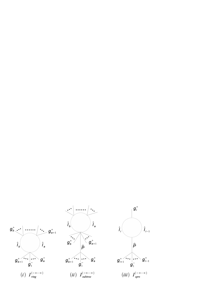
Figure 1: Diagrams contributing to the one-loop one-minus amplitudes of $n$ gluons

Following the notation in [22], the EFK result for the $n$-point one-loop one-minus amplitudes/integrands can be summarized as

$$I^{(1_{-}2_{+}3_{+}\cdots n_{+})}\,=\,I^{(-+\cdots+)}_{ring}+I^{(-+\cdots+)}_{subtree}+I^{(-+\cdots+)}_{sprs}\,,$$ (5.13)

where the terms in the right-hand side respectively correspond to the diagrams in Figure 1 and are explicitly given by

$$I^{(-+\cdots+)}_{ring} = \sum_{a<b}\frac{-2N_{p}m^{2}(1l_{a})^{2}(1l_{b})^{2}(a\,a+1)(b\,b+1)}{(12)(23)\cdots(n1)\,(l_{a}l_{b})(al_{a})(l_{a}\,a+1)(bl_{b})(l_{b}\,b+1)}\frac{i}{\widehat{l}_{a}^{2}-m^{2}}\frac{i}{\widehat{l}_{b}^{2}-m^{2}}$$ (5.14)

$$~{}~{}~{}\times\left(l_{a}\left|\prod_{j=a+1}^{b-1}\left[1-\frac{im^{2}|l_{j})(j\,j+1)(l_{j}|}{(\widehat{l}_{j}^{2}-m^{2})(j\,l_{j})(l_{j}\,j+1)}\right]\right|l_{b}\right)\,,$$

$$I^{(-+\cdots+)}_{subtree} = \sum_{2\leq b-a\leq n-2}\frac{(1P)^{4}}{(P\,b+1)(b+1\,b+2)\cdots(a-1\,a)(aP)}$$ (5.15)

$$~{}~{}~{}~{}~{}~{}~{}~{}~{}~{}~{}~{}~{}~{}\times\,\frac{i}{\widehat{P}^{2}}~{}I^{(++\cdots+)}_{CSW}(a+1,\cdots,b,P)\,,$$

$$I^{(-+\cdots+)}_{sprs} = \sum_{i=2}^{n}\frac{-2N_{p}m^{2}}{(12)(23)\cdots(n1)}\frac{\sqrt{-1}}{\widehat{l}_{i}^{2}-m^{2}}\frac{\sqrt{-1}}{\widehat{l}_{i-1}^{2}-m^{2}}\frac{(1i)^{2}}{(il_{i})}$$ (5.16)

$$~{}~{}~{}\times\left[\frac{(1l_{i-1})(1l_{i})}{(il_{i})}-\frac{(1\,i-1)(1l_{i})}{(i-1\,i)}+\frac{(1\,i+1)(1l_{i-1})}{(i\,i+1)}\right]\,.$$

In (5.15) the one-loop all-plus integrand $I^{(++\cdots+)}_{CSW}(a+1,\cdots,b,P)$ is defined as a trace over the UHV tree amplitudes:

$$I^{(++\cdots+)}_{CSW}(a+1,\cdots,b,P) = \frac{2N_{p}}{(a+1\,a+2)(a+2\,a+3)\cdots(bP)(P\,a+1)}$$ (5.17)

$$\times\,{\rm Tr}^{\prime}\prod_{j=a+1}^{P}\left[1-\frac{im^{2}|l_{j})(j\,j+1)(l_{j}|}{(\widehat{l}_{j}^{2}-m^{2})(j\,l_{j})(l_{j}\,j+1)}\right]$$

where the trace is taken over the two-component spinors and ${\rm Tr}^{\prime}$ is defined as ${\rm Tr}^{\prime}X\equiv{\rm Tr}X-{\rm Tr}{\bf 1}$ to subtract the identity factor ${\rm Tr}{\bf 1}=2$ from (5.17). In the expressions (5.14)-(5.17), the overall prefactor $N_{p}$ is introduced in order to make the pure gluonic amplitudes to those of QCD including (massless) fermion contributions in the loop. Neglecting the fermion contributions, we can set $N_{p}=1$.

To obtain the NUHV tree amplitudes from these EFK results of the one-loop one-minus QCD amplitudes, we should bear in mind the following two things.

1. One is the fact that in a one-loop (MHV) diagram we can make at least one leg on each side of the diagram be collinear to each other. This is due to the freedom we have in the choice of the reference spinors involving the loop propagators. This is also a useful lesson we have learned from the one-loop calculations of ${\cal N}=4$ super Yang-Mills theory in the holonomy formalism, see [28] for details.

2. The other thing is, as mentioned earlier, that the reference spinors involved in the EFK results (5.13)-(5.17) are not specified. This has been convenient to study the freedom from spurious poles in the one-loop amplitudes [22]. However, for our purposes, i.e. to compare our formulation of the NUHV tree amplitudes (5.2) to the EFK results (5.13)-(5.17), we no longer need to keep the reference spinors arbitrary. We can fix them in a suitable way before reducing the EFK results to the NUHV tree amplitudes.

From the first condition, we can easily find that the ring integrand $I^{(-+\cdots+)}_{ring}$ vanishes upon the choice of $u_{a}\parallel u_{a+1}$, i.e., $(a\,a+1)=0$. The first condition also implies that diagram $(iii)$ in Figure 1 can be treated as a tadpole-like diagram. This means that the integrand $I^{(-+\cdots+)}_{sprs}$ can be considered as a UHV-MHV type amplitude upon the reduction to the NUHV tree amplitude by cutting the massive loop apart. The UHV part of the tree amplitude then has the minimum three legs composed of two massive scalars and one internal virtual gluon (but no pure gluons). Similarly, we can reduce the subtree integrand $I^{(-+\cdots+)}_{subtree}$ to UHV-MHV type amplitudes upon cutting the massive loop apart. The UHV part of the reduced NUHV tree amplitudes have more than three legs (including an arbitrary number of gluons). These analyses show that the EFK representation for the NUHV tree amplitudes is given in terms of UHV and MHV vertices connected by massive scalar propagators. This description agrees with our construction of the NUHV tree amplitudes (5.2). In fact, installing information of color factors and permutation invariance under gluon transpositions, we find that the above EFK representation of the NUHV tree amplitudes exactly agrees with our formulation (5.2).

Generalization to non-UHV tree amplitudes

Field theoretically it is straightforward to obtain non-UHV tree amplitudes out of the S-matrix functional for massive scalar amplitudes in (5.1). We simply apply a sequence of functional derivatives of interest to the S-matrix functional and evaluate the derivatives as in (4.41). Because of the contraction operators the computation is entirely based on the massless and massive CSW rules except that we make use of vanishing non-UHV vertices (4.18), (4.19) in the massive part, rather than the original proposal (4.15), (4.16). As in the cases of non-MHV gluon amplitudes, we can hence obtain non-UHV massive scalar amplitudes in terms of the UHV and the MHV vertices or what we previously call the “UHV rules.” An explicit form of the non-UHV amplitudes are as tedious and complicated as that of the non-MHV amplitudes. From the S-matrix functional (5.1), however, we can easily obtain a succinct recursive expression for the non-UHV tree amplitudes:

$$\widehat{A}_{\rm N^{k}UHV(0)}^{({\bar{\phi}}_{1}g_{a_{1}}^{-}g_{a_{2}}^{-}\cdots g_{a_{k}}^{-}\phi_{n})}(u)$$ (5.18)

$$= \left.\sum_{i=2}^{n-1}\sum_{r=1}^{n-3}\widehat{A}^{((i+r+1)_{+}\cdots\phi_{n}\bar{\phi}_{1}\cdots(i-1)_{+}l_{+})}_{\rm UHV(0)}(u)\,\frac{1}{q_{i\,i+r}^{2}}\,\widehat{A}^{((-l)_{-}\,(i)_{+}\cdots a_{1-}\cdots a_{2-}\cdots\cdots a_{k-}\cdots(i+r)_{+})}_{\rm N^{k-1}MHV(0)}(u)\right|_{u_{l}=u_{i\,i+r}}$$

where $k=1,2,\cdots,n-3$ and the meanings of $q_{i\,i+r}$ and $u_{l}$ are the same as in (5.2).

Alternatively, we can also express the N^kUHV massive scalar amplitudes as

$$\widehat{A}_{\rm N^{k}UHV(0)}^{({\bar{\phi}}_{1}g_{a_{1}}^{-}g_{a_{2}}^{-}\cdots g_{a_{k}}^{-}\phi_{n})}(u)$$ (5.19)

$$= \left.\sum_{i=2}^{n-1}\sum_{r=1}^{n-3}\widehat{A}^{((i+r+1)_{+}\cdots\phi_{n}\bar{\phi}_{1}\cdots(i-1)_{+}l_{+})}_{\rm N^{k-1}UHV(0)}(u)\,\frac{1}{q_{i\,i+r}^{2}}\,\widehat{A}^{((-l)_{-}\,(i)_{+}\cdots a_{k-}\cdots(i+r)_{+})}_{\rm MHV(0)}(u)\right|_{u_{l}=u_{i\,i+r}}$$

where we make the negative-helicity indices implicit in $\widehat{A}^{((i+r+1)_{+}\cdots\phi_{n}\bar{\phi}_{1}\cdots(i-1)_{+}l_{+})}_{\rm N^{k-1}UHV(0)}(u)$. The latter expression (5.19) is recursive in terms of the massive part of the massive amplitudes, while the former (5.18) is in terms of the gluonic part of them. The gluonic N^kMHV tree amplitudes in (5.18) can be constructed by the original massless CSW rules, while the massive N^kUHV tree amplitudes in (5.19) is constructed only from the N^k-1UHV counterpart in an inductive way. In this sense the two expressions reveal the structure behind the CSW rules and the BCFW recursion methods and indicate their equivalence in the calculations of the massive scalar amplitudes at tree level.

Lastly we should comment on loop effects to the massive scalar amplitudes. As noted earlier, massive loop effects arise in purely gluonic part of the massive scalar amplitudes. For example, we can incorporate one-loop all-plus gluon configurations into the gluonic part of the UHV amplitudes. There are also massless loop effects contributing to the general gluon amplitudes. Therefore, taking the expression (5.18) for instance, we can in principle calculate the one-loop massive scalar amplitudes as

$$\widehat{A}_{\rm N^{k}UHV(1)}^{({\bar{\phi}}_{1}g_{a_{1}}^{-}g_{a_{2}}^{-}\cdots g_{a_{k}}^{-}\phi_{n})}(u)$$ (5.20)

$$= \sum_{i=2}^{n-1}\sum_{r=1}^{n-3}\left[\widehat{A}^{((i+r+1)_{+}\cdots\phi_{n}\bar{\phi}_{1}\cdots(i-1)_{+}l_{+})}_{\rm UHV(1)}(u)\,\frac{1}{q_{i\,i+r}^{2}}\,\widehat{A}^{((-l)_{-}\,(i)_{+}\cdots a_{1-}\cdots a_{2-}\cdots\cdots a_{k-}\cdots(i+r)_{+})}_{\rm N^{k-1}MHV(0)}(u)\right.$$

$$~{}~{}~{}+\,\left.\widehat{A}^{((i+r+1)_{+}\cdots\phi_{n}\bar{\phi}_{1}\cdots(i-1)_{+}l_{+})}_{\rm UHV(0)}(u)\,\frac{1}{q_{i\,i+r}^{2}}\,\widehat{A}^{((-l)_{-}\,(i)_{+}\cdots a_{1-}\cdots a_{2-}\cdots\cdots a_{k-}\cdots(i+r)_{+})}_{\rm N^{k-1}MHV(1)}(u)\right]_{u_{l}=u_{i\,i+r}}$$

From this expression we may obtain explicit forms of the one-loop massive scalar amplitudes but that task is beyond the scope of the present paper and we shall leave it to future works.

6 Concluding remarks

One of the main purposes of this paper is to investigate whether an off-shell continuation of Nair’s superamplitude method can be applied to a massive model, particularly to amplitudes of an arbitrary number of gluons and a pair of massive scalars (or massive scalar amplitudes), in a framework of the holonomy formalism. In the present paper we have affirmed this proposition by making a specific choice of the reference spinors for the massive scalars, see (4.20). This allows us to obtain a functional derivation of the so-called ultra helicity violating (UHV) vertices (4.14) of the massive scalar amplitudes, eventually leading us to the S-matrix functional (5.1) for the massive scalar amplitudes in general.

An essential ingredient of the S-matrix functional is given by the massive holonomy operator $\Theta_{R,\gamma}^{(B)}(u)$ we have defined in section 3. This operator is relevant to the generation of the massive part of the massive scalar amplitudes. In particular, together with the contraction operator $\widehat{W}^{(0)}(x)$ in (4.37), this operator generates the UHV tree amplitudes (4.41)-(4.45) in a form that was previously reported by Kiermaier [21], using the so-called massive CSW rules of Boels and Schwinn [15, 16].

One of the interesting features in our formulation is that a careful analysis of the braid trace in the construction of $\Theta_{R,\gamma}^{(B)}(u)$ leads to no apparent sums over permutations of gluons in the color structure of the UHV tree amplitudes, or the massive part of the massive scalar amplitudes in general. The number of terms involving the UHV tree amplitudes, however, does not drastically decrease from that of the MHV tree amplitudes of gluons. This is due to the fact that actions of the contraction operator $\widehat{W}^{(0)}(x)$ do not alter the gluon helicity configurations for the massive scalar amplitudes. We have briefly presented a quantitative analysis of this fact in (4.35) and below.

The holonomy formalism is neither Lagrangian nor Hamiltonian formalism so that we do/can not introduce potentials for the incorporation of massive particles. Information of mass is embedded into physical operators such that helicity or polarization of the particles of interest is in accord with the definition of the helicity operator (2.31). In practice, this can be carried out by considering an off-shell continuation of Nair’s superamplitude method. In the present paper we strictly follow this idea, with its concrete realization given in (4.6). Notice that our approach is philosophically different from other approaches found in the literature. For example, the massive CSW rules [15, 16] are derived from the Lagrangian formalism [32]-[36]. The earlier approaches [4]-[11], on the other hand, focus more on the application of the CSW rules or the BCFW recursion relations to massive models and its usage rather than its derivation from first principles. The holonomy formalism is therefore qualitatively new in the studies of massive scalar amplitudes and possibly leads to a completely new mass generation mechanism. Obviously it is worth investigating how massive fermions and massive bosons will be incorporated into the same framework. We shall consider such extensions in a forthcoming paper.

Lastly, we would like to emphasize that in our formalism mass effects do not invoke supersymmetry breaking. The full ${\cal N}=4$ supersymmetry has been crucial to derive the correct form of the UHV vertex (4.14) which forms a basic building block for the massive scalar amplitudes. (Such a construction is referred to as the “UHV rules” in the above text.) As explicitly shown in (4.23)-(4.26), the derivation is given in a conventional functional method. Thus the holonomy formalism can naturally be continued to a massive model without breaking the extended ${\cal N}=4$ supersymmetry. It would be useful to take account of this fact in the construction of more realistic massive models in the framework of holonomy formalism or, more broadly, in the four-dimensional spinor-helicity formalism.

References

[1]
F. Cachazo, P. Svrcek and E. Witten,
JHEP 0409, 006 (2004)
[arXiv:hep-th/0403047].
[2]
R. Britto, F. Cachazo and B. Feng,
Nucl. Phys. B 715, 499 (2005)
[arXiv:hep-th/0412308].
[3]
R. Britto, F. Cachazo, B. Feng and E. Witten,
Phys. Rev. Lett. 94, 181602 (2005)
[arXiv:hep-th/0501052].
[4]
L. J. Dixon, E. W. N. Glover and V. V. Khoze,
JHEP 0412, 015 (2004)
[arXiv:hep-th/0411092].
[5]
S. D. Badger, E. W. N. Glover and V. V. Khoze,
JHEP 0503, 023 (2005)
[arXiv:hep-th/0412275].
[6]
Z. Bern, D. Forde, D. A. Kosower and P. Mastrolia,
Phys. Rev. D 72, 025006 (2005)
[arXiv:hep-ph/0412167].
[7]
S. D. Badger, E. W. N. Glover, V. V. Khoze and P. Svrcek,
JHEP 0507, 025 (2005)
[arXiv:hep-th/0504159].
[8]
S. D. Badger, E. W. N. Glover and V. V. Khoze,
JHEP 0601, 066 (2006)
[arXiv:hep-th/0507161].
[9]
D. Forde and D. A. Kosower,
Phys. Rev. D 73, 065007 (2006)
[hep-th/0507292].
[10]
G. Rodrigo,
JHEP 0509, 079 (2005)
[hep-ph/0508138].
[11]
P. Ferrario, G. Rodrigo and P. Talavera,
Phys. Rev. Lett. 96, 182001 (2006)
[hep-th/0602043].
[12]
Z. Bern, L. J. Dixon, D. A. Kosower, S. Weinzierl,
Nucl. Phys. B489, 3-23 (1997)
[hep-ph/9610370].
[13]
L. J. Dixon, Z. Kunszt and A. Signer,
Nucl. Phys. B 531, 3 (1998)
[arXiv:hep-ph/9803250].
[14]
S. Dittmaier,
Phys. Rev. D59, 016007 (1998).
[arXiv:hep-ph/9805445 [hep-ph]].
[15]
R. Boels and C. Schwinn,
Phys. Lett. B 662, 80 (2008)
[arXiv:0712.3409 [hep-th]].
[16]
R. Boels and C. Schwinn,
JHEP 0807, 007 (2008)
[arXiv:0805.1197 [hep-th]].
[17]
S. Buchta, S. Weinzierl,
JHEP 1009, 071 (2010)
[arXiv:1007.2742 [hep-ph]].
[18]
T. Cohen, H. Elvang and M. Kiermaier,
JHEP 1104, 053 (2011)
[arXiv:1010.0257 [hep-th]].
[19]
N. Craig, H. Elvang, M. Kiermaier, T. Slatyer,
[arXiv:1104.2050 [hep-th]].
[20]
R. H. Boels and C. Schwinn,
Phys. Rev. D 84, 065006 (2011)
[arXiv:1104.2280 [hep-th]].
[21]
M. Kiermaier,
arXiv:1105.5385 [hep-th].
[22]
H. Elvang, D. Z. Freedman and M. Kiermaier,
arXiv:1111.0635 [hep-th].
[23]
J. -H. Huang and W. Wang,
arXiv:1204.0068 [hep-th].
[24]
C. Schwinn and S. Weinzierl,
JHEP 0603, 030 (2006)
[hep-th/0602012].
[25]
Y. Abe,
Nucl. Phys. B 825, 242 (2010)
[arXiv:0906.2524 [hep-th]].
[26]
Y. Abe,
Nucl. Phys. B 825, 268 (2010)
[arXiv:0906.2526 [hep-th]].
[27]
Y. Abe,
Nucl. Phys. B 842, 475 (2011)
[arXiv:1008.2800 [hep-th]].
[28]
Y. Abe,
Nucl. Phys. B 854, 193 (2012)
[arXiv:1105.6146 [hep-th]].
[29]
T. Kohno, Conformal Field Theory and Topology, Translations of
Mathematical Monographs, Volume 210, American Mathematical Society (2002).
[30]
L. S. Cirio and J. F. Martins,
arXiv:1106.0042 [hep-th].
[31]
V. P. Nair,
Phys. Lett. B 214, 215 (1988).
[32]
A. Gorsky and A. Rosly,
JHEP 0601, 101 (2006)
[hep-th/0510111].
[33]
P. Mansfield,
JHEP 0603, 037 (2006)
[hep-th/0511264].
[34]
J. H. Ettle and T. R. Morris,
JHEP 0608, 003 (2006)
[hep-th/0605121].
[35]
L. J. Mason,
JHEP 0510, 009 (2005)
[arXiv:hep-th/0507269].
[36]
R. Boels, L. Mason and D. Skinner,
Phys. Lett. B 648, 90 (2007)
[arXiv:hep-th/0702035].