Effective-Range Dependence of Resonantly Interacting Fermions

Abstract

We extract the leading effective range corrections to the equation of state of the unitary Fermi gas from ab initio calculations in a periodic box using a , and show them to be universal by considering several two-body interactions. Furthermore, we find that the is consistent with the best available unbiased calculations, analytic results, and experimental measurements of the equation of state. We also discuss the asymptotic effective-range corrections for trapped systems and present the first results with the correct asymptotic scaling.

The fermion many-body problem plays a fundamental role in a vast array of physical systems, from dilute gases of cold atoms to nuclear physics in nuclei and neutron stars. The universal character of this problem – each system is governed by a similar microscopic theory – coupled with direct experimental access in cold atoms, has led to an explosion of recent interest (see Refs. IKS:2008; *giorgini-2007; *Zwerger:2011 for reviews). Despite this broad applicability, we still do not fully understand even the simplest system: the “unitary gas” comprising equal numbers of two fermionic species with a resonant $s$-wave interaction of infinite scattering length $a_{s}\to\infty$. Lacking any scale beyond the total density $n_{+}=n_{a}+n_{b}$, the unitary gas admits no perturbative expansion and requires experimental measurement or accurate numerical simulation for a quantitative description. Typical calculations, however, can access at most a few hundred particles, while experiments can measure only a handful of properties. provides a complementary approach through which one may extrapolate these results to large systems beyond the reach of direct simulation. The question of how the unitary gas approaches the thermodynamic limit has also been studied in Morris:2010; FGG:2010; Li:2011; Braun:2011.

In this paper, we consider the effects of a finite effective range $r_{e}$ on the unitary gas. Our motivation is two-fold. First, neutron matter – well approximated by a unitary gas Gezerlis;Carlson:2008-03 – differs primarily due to a finite range. Characterizing the finite range effects therefore have physical relevance. Second, we wish to directly use a – a finite-range version of the – to fit simulations and extract thermodynamic properties without having to first extrapolate to zero range as was done in FGG:2010. Directly fitting the finite range data provides a much more stringent test of the . We use this finite-range to extrapolate to the thermodynamic limit the linear range dependence of the equation of state, and demonstrate its universality by simulating three different potentials. Two of the potentials include a repulsive core to address issues of contamination by deep bound states. We also show that the consistently fits all available unbiased zero-range ab initio results for the symmetric unitary gas. Finally, we present results for trapped systems that demonstrate the correct asymptotic scaling as predicted by the low energy effective theory for the unitary gas.

Here we consider symmetric $T=0$ systems comprising equal numbers of two neutral Fermi species with equal mass with a short-range interaction. These systems are directly realized by two of the lowest lying hyperfine states of ^6Li in cold atomic systems, and approximately realized in dilute neutron-rich matter in the crusts of neutron stars. At sufficient dilution, the interaction can be characterized by the two-body s-wave phase shifts through the effective range expansion (see for example Bethe:1949)

$$k\cot\delta_{k}=\frac{-1}{a_{s}}+\frac{r_{e}k^{2}}{2}+\mathcal{O}(k^{4})$$ (1)

where $a_{s}$ is the s-wave scattering length and $r_{e}$ is the effective range. The zero-range unitary limit is realized when the scattering length is tuned $a_{s}\rightarrow\infty$ and the system is diluted such that $kr_{e}\rightarrow 0$: this is referred to as the symmetric .

The lack of scales implies that the symmetric is fully characterized by the universal Bertsch parameter mbx; *Baker:1999:PhysRevC.60.054311; *baker00:_mbx_chall_compet $\xi_{S}=\mathcal{E}/\mathcal{E}_{FG}$, where $\mathcal{E}_{FG}=(3/5)n_{+}E_{F}$ is the energy density of a free Fermi gas with the same total density $n_{+}=k_{F}^{3}/(3\pi^{2})$, and $E_{F}=\hslash^{2}k_{F}^{2}/2m$ is the Fermi energy.

In ^6Li cold-atom experiments (see Ku:2011 for details), $a_{s}\approx\infty$ can be tuned using the wide magnetic Feshbach resonance at $834.1(15)\text{\,}\mathrm{G}$ Bartenstein:2005uq with an effective range of $r_{e}\approx$4.7\text{\,}\mathrm{n}\mathrm{m}$$, while the gas can be cooled at densities of $1/k_{F}\approx$400\text{\,}\mathrm{n}\mathrm{m}$$ so that $k_{F}r_{e}\approx 0.01$. In dilute neutron matter $a_{nn}\approx$-18.9(4)\text{\,}\mathrm{f}\mathrm{m}$$ Gonzalez-Trotter:2006; *Chen:2008 and $r_{nn}\approx$2.75(11)\text{\,}\mathrm{f}\mathrm{m}$$ Miller:1990, while densities are on the order of $1/k_{F}\sim$1\text{\,}\mathrm{f}\mathrm{m}$$: thus, $k_{F}r_{e}\approx 3$ is several orders of magnitude larger than in cold-atom systems.

Although there are formal ways of dealing with the divergences introduced by the zero-range limit (see Tan:2005uq; *Tan:2008kx; *Tan:2008uq for an interesting approach), most ab initio calculational techniques require an explicit regulator in the form of a finite-range potential or a lattice cutoff. To extract the unitary parameters thus requires an extrapolation to zero effective range. Range effects in the are also discussed in Schwenk:2005ka (large $r_{e}$), Li:2011 (), and in Simonucci:2011; Caballero-Benitez:2012 ( approximation).

I Summary

Here we present a summary of our results. We use a variational algorithm to find upper bounds on the energy for systems of $4$ to $66$ particles in a periodic box for a variety of effective ranges $k_{F}r_{e}\lessapprox 0.3$ and for different potentials with the same scattering length $a_{s}=\infty$ and range. We fit these directly with a modified that models the range dependence in order to extrapolate to the thermodynamic an upper bound on the Bertsch parameter $\xi$, and the leading order universal effective range dependence $\zeta_{e}$:

$$\xi(k_{F}r_{e})\lessapprox\xi^{*}+\zeta_{e}^{*}k_{F}r_{e}+\mathcal{O}(k_{F}r_{e})^{2}$$

$$\begin{aligned} \xi^{*}&=0.3897(4)&\zeta_{e}^{*}&=0.127(4).\end{aligned}$$ (2a)

By comparing several potentials, we confirm that these are indeed universal. The results contain a systematic error due to the variational nature of the method. To better understand this, we also fit with the a collection of unbiased exact, , and experimental results for systems with $$2 10^{6}$$ to particles, obtaining a best fit of

$$\xi_{S} =$0.3742(5)$.$$ (2b)

We also demonstrate for the first time, results for trapped systems that exhibit the correct asymptotic behavior in the thermodynamic limit.

II Model

We use a algorithm to simulate the Hamiltonian

$$\mathcal{H}=\frac{\hslash^{2}}{2m}\Biggl{(}-\sum\limits_{k=1}^{N_{+}}\nabla_{k}^{2}\;-\;\sum_{i,j^{\prime}}V(r_{ij^{\prime}})\Biggr{)},$$ (3)

where $V(r)$ is an inter-species interaction (off-resonance intra-species interactions are neglected). The algorithm projects out the state of lowest energy from the space of all wave functions with fixed nodal structure as defined by an initial many-body wave function (ansatz). By varying the Ansatz, we obtain an upper bound on the ground-state energy.

We use the trial function introduced in CCPS:2003:

$$\Psi_{T}=\mathcal{A}[\phi(\mathbf{r}_{11^{\prime}})\phi(\mathbf{r}_{22^{\prime}})\cdots\phi(\mathbf{r}_{nn^{\prime}})]\prod_{ij^{\prime}}f(r_{ij^{\prime}}),$$

where $\mathcal{A}$ antisymmetrizes over particles of the same spin (either primed or unprimed) and $f(r)$ is a nodeless Jastrow function introduced to reduce the statistical error. The antisymmetrized product of $s$-wave pairing functions $\phi(\mathbf{r}_{ij^{\prime}})$ defines the nodal structure:

$$\phi(\mathbf{r})=\sum_{\mathbf{n}}\alpha_{\lVert\mathbf{n}\rVert}e^{i{\mathbf{k}}_{\mathbf{n}}\cdot\mathbf{r}}+\tilde{\beta}(r).$$

The sum is truncated (we include ten coefficients) and the omitted short-range tail is modelled by the phenomenological function $\tilde{\beta}(r)$ chosen to ensure smooth behavior near zero separation. We use the same form for $\tilde{\beta}(r)$ as in Gandolfi:2010a and vary the 10 coefficients $\alpha_{\lVert\mathbf{n}\rVert}$ for each $N_{+}$ and for each different two-body potential to minimize the energy as described in Ref. Sorella:2001. The same ansatz suffices for different effective ranges, but an independent optimization is required for each $N_{+}$.

We compare the following potentials:

$$V_{PT}(r) =4\mu^{2}\operatorname{sech}^{2}(\mu r),$$ (4a)

$$V_{2G}(r) =$3.144\,390\,429\,149\,88$\mu^{2}\left(e^{-\mu^{2}r^{2}/4}-4e^{-\mu^{2}r^{2}}\right),$$ (4b)

$$V_{2E}(r) =$4.763\,660\,471\,866\,52$\mu^{2}\left(e^{-\mu r}-2e^{-2\mu r}\right).$$ (4c)

These potentials are all tuned to have infinite two-body $s$-wave scattering length. The first potential (4a) is of the modified–Pöschl-Teller type; the second (4b) and third (4c) potentials have a repulsive core. When tuned to unitarity, the effective range $r_{e}$ is proportional to $\mu^{-1}$ as shown in figure 1.

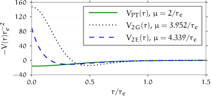
Figure 1: (color online) Finite range potentials (4) used in the Hamiltonian (3) for our bounds.

One criticism of purely attractive potentials – including the widely used modified–Pöschl-Teller potential (4a) – is that they may contain deeply bound states where many particles lie within the range of the potential. Formally, the ground state is thus not the universal dilute , but some tightly bound state that is highly sensitive to the range. In principle, this state may contaminate the variational calculation, but in practice, there is insufficient overlap between the variational wave function and this deep bound state. (Simulations longer by several orders of magnitude would be required to see the influence of such low-energy states.)

The repulsive cores of (4b) and (4c) help allay these concerns by reducing the possibility of contamination from deeply bound states. We find agreement between the purely attractive Pöschl-Teller potential and these repulsive potentials, demonstrating that all three potentials may be used to calculate properties of the , and verifying the model-independence of the universal parameters. We show the upper bounds for the energy of $N_{+}=66$ particles at various effective ranges in figure 2. For ranges less than $k_{F}r_{e}\lesssim 0.3$ a three-parameter quadratic model is sufficient to extrapolate to zero range without a systematic bias. This fit is shown in table 1 for the three potentials, and the magnitude of the quadratic parameter can be used to estimate the linear regime.

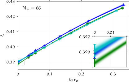
Figure 2: (color online) Effective range dependence of the ground-state energy-density $\xi(k_{F}r_{e})=\mathcal{E}/\mathcal{E}_{FG}$ of $N_{+}=66$ fermions in a periodic cubic box in the unitary limit. The points with error-bars are the raw results and the bands are the $1\sigma$ error bands of polynomial fits. The upper (blue) curve that extrapolates to $\xi=$0.3898(5)$$ is the new quadratic fit to the modified–Pöschl-Teller potential (4a). The middle (green) curve that extrapolates to $\xi=$0.3885(5)$$ is the quadratic fit for the new double-Gaussian potential (4b). Finally, the lower (cyan) curve that extrapolates to $\xi=$0.3902(7)$$ is the quadratic fit to the double-exponential potential (4c).

	$\xi_{66}$ ($=a_{0}$)	$\zeta_{e}(66)$ ($=a_{1}$)	$a_{2}$	$\chi^{2}_{\text{r}}$
$V_{PT}$	$0.3898(4)$	$0.14(1)$	$-0.07$	$0.2$
$V_{2G}$	$0.3885(4)$	$0.14(1)$	$-0.08$	$0.4$
$V_{2E}$	$0.3902(5)$	$0.12(1)$	$-0.03$	$0.3$

Table 1: Comparison of the zero-range extrapolations of $\mathcal{E}(k_{F}r_{e})/\mathcal{E}_{FG}=\xi_{66}+\zeta_{e}(66)k_{F}r_{e}+a_{2}(k_{F}r_{e})^{2}+\mathcal{O}(r_{e}^{3})$ for quadratic fits of the $N_{+}=66$ results. These values are higher than, but consistent with the value $\zeta_{e}(66)=$0.11(3)$$ reported in Carlson:2011. The extrapolations of these parameters to the thermodynamic limit $N_{+}=\infty$ are listed as $\xi=a_{0}$ and $\zeta_{e}=a_{1}$ in the $\xi$ block of table LABEL:tab:thermo. We include the quadratic coefficient simply to show that the can be fit using a linear form for $k_{F}r_{e}<\epsilon_{\text{abs}}\lvert{a_{1}/a_{2}}\rvert$ to an absolute accuracy of about $\epsilon_{\text{abs}}$: we do not have any a priori reason to believe that this parameter is universal. The systematic error due to neglecting the cubic terms is on the same order as the quoted $1\sigma$ statistical errors.

In FGG:2010, each $N_{+}$ was independently extrapolated to zero effective range, then the unitary was fit to the extrapolated results. It was claimed that a cubic fit was required to extrapolate the results for $k_{F}r_{e}<0.35$ to zero range, however, the smallest ranges $k_{F}r_{e}<0.1$ had a small systematic bias in the energy due to the Trotter decomposition of the many-body propagator $e^{-\hat{H}\delta\tau}\approx e^{-\hat{V}\delta\tau/2}e^{-\hat{K}\delta\tau}e^{-\hat{V}\delta\tau/2}+\mathcal{O}(\hat{V}\delta\tau)^{3}$ where $\delta\tau/\hslash$ is the imaginary time-step. Since the potentials (4) scale roughly as $\hat{V}\propto\mu^{2}\propto r_{e}^{-2}$, for small ranges, one needs a very small imaginary time-step, which is computationally expensive. The extrapolated values of $\xi$ were only underestimated for the larger systems (by $\sim 3\%$), but extracting the slope of $\xi(k_{F}r_{e})$ requires higher accuracy. Here we have carefully simulated with smaller time-steps (for the ranges considered here, $\delta\tau E_{F}\approx 5\times 10^{-6}$ is sufficient to avoid any bias) to find that, for $k_{F}r_{e}\lessapprox 0.3$, a quadratic (but not linear) fit is sufficient. We also no longer use an independent zero-range extrapolation for each $N_{+}$. Instead, we use a generalized finite-range– to fit all of the finite-range– results with a common set of parameters. This requires simultaneous consistency over all ranges and all particle numbers, providing a more rigorous test than independently extrapolating each $N_{+}$.

III with Finite Range

As was shown in FGG:2010, the finite-size (“shell”) effects in $\xi_{S}(N_{+})$ can be well modelled by a simple local for the unitary Fermi gas, but are not even qualitatively reproduced by adding only gradient or kinetic corrections Papenbrock:2005fk; Rupak:2008fk; Salasnich:2008. In this paper we retain the same three-parameter form originally introduced in Ref. Bulgac:2007a (called the ), but present a simple generalization that accounts for finite-range effects. With this generalized form, we can directly fit the results without the need to first extrapolate to zero range. We first briefly review the form of the , then discuss the finite-range generalization.

The is formulated in terms of three local densities (see Bulgac:2011 for a review): the total density $n_{+}$, the total kinetic density $\tau_{+}$, and an anomalous $\nu$:

$$n_{+} =2\sum_{n}\lvert{v_{n}}\rvert^{2}\sim\langle\hat{a}^{\dagger}\hat{a}\rangle+\langle\hat{b}^{\dagger}\hat{b}\rangle,$$

$$\tau_{+} =2\sum_{n}\lvert{\nabla v_{n}}\rvert^{2}\sim\langle\vec{\nabla}\hat{a}^{\dagger}\cdot\vec{\nabla}\hat{a}\rangle+\langle\vec{\nabla}\hat{b}^{\dagger}\cdot\vec{\nabla}\hat{b}\rangle,$$

$$\nu =\sum_{n}u_{n}v_{n}^{*}\sim\langle\hat{a}\hat{b}\rangle.$$

These are expressed in terms of the Bogoliubov quasiparticle wave functions $u_{n}(\mathbf{r})$ and $v_{n}(\mathbf{r})$ – sometimes called “coherence factors”.

The three-parameter may then be expressed as

$$\mathcal{E}=\frac{\hslash^{2}}{m}\left(\frac{\alpha}{2}\tau_{+}+\beta\frac{3}{10}(3\pi^{2})^{2/3}n_{+}^{5/3}\right)+g\nu^{\dagger}\nu,$$

where $\alpha=m/m_{\text{eff}}$ parametrizes the inverse effective mass; $\beta$ parametrizes the self-energy; and $g$ parametrizes the pairing interaction. In the presence of pairing, the local kinetic and anomalous densities are divergent

$$\lim_{\delta\rightarrow 0}\nu(\vec{x},\vec{x}+\vec{\delta}) \rightarrow\frac{A_{\nu}}{\delta}+\nu_{r}(\vec{x})+\mathcal{O}(\delta),$$

$$\lim_{\delta\rightarrow 0}\tau_{+}(\vec{x},\vec{x}+\vec{\delta}) \rightarrow\frac{A_{\tau}}{\delta}+\tau_{r}(\vec{x})+\mathcal{O}(\delta),$$

where $A_{\nu}$, $A_{\tau}$, $\nu_{r}$ and $\tau_{r}$ are finite. One must regulate the theory if one wishes to maintain a local formulation, which greatly simplifies the computational aspects of the . The most general form of a local functional involving these three densities is a function of these four finite quantities, but restricting the form to bounded functionals is somewhat non-trivial Forbes:2012a, and we shall not consider these generalizations here.

We note that the $1/\delta$ divergence corresponds to a long $1/k^{2}$ momentum tail in the Fourier transform of the anomalous and kinetic densities. This follows from the short-range nature of the potential as has been emphasized by Tan Tan:2005uq; *Tan:2008kx; *Tan:2008uq. The most straightforward route is to simply introduce a momentum cutoff $k<k_{c}$ and then define the theory in the limit of large cutoff. The local densities then behave as

$$\tau_{+} =A_{\tau}\Lambda+\tau_{r}+\mathcal{O}(\Lambda^{-1}), \nu =A_{\nu}\Lambda+\nu_{r}+\mathcal{O}(\Lambda^{-1}),$$

where $\Lambda=\int k^{-2}\mathrm{d}^{3}{k}/(2\pi)^{3}=k_{c}/2\pi^{2}$. Within the single-particle framework of the , these are related to the gap $\Delta$: $A_{\tau}=2m\lvert{\Delta}\rvert^{2}/\alpha^{2}$, and $A_{\nu}=\Delta/\alpha$. Similar short-range behavior is expected in the physical density distributions where the coefficients $A_{\tau}$ and $A_{\nu}$ are related to the Tan’s “contact” $C$ – for example, $A_{\nu}=\sqrt{2C}/2m$ – and it is tempting to interpret $\sqrt{2C}\approx 2m\Delta/\alpha$ as a prediction of the , especially at unitarity where they seem to be related numerically. This cannot hold in general: in particular, the contact $C$ is related to the short-range nature of the interaction and persists in the normal phase (either meta-stable or above the critical temperature $T>T_{c}$) where the order parameter $\Delta$ vanishes Tan:pc. The inverse coupling constant may be expressed

$$g^{-1}=n_{+}^{1/3}/\gamma-\Lambda/\alpha,$$

where $\gamma$ is the third dimensionless parameter characterizing the .

The equations of motion follow by minimizing the total energy $E=\int\mathrm{d}^{3}{x}\;\mathcal{E}_{SLDA}$ with respect to the occupation factors $u$ and $v$ subject to the constraints of fixed total particle number $N_{+}$ and normalization. This leads to the following single-particle Hamiltonian for the Bogoliubov quasiparticle wavefunctions:

$$\begin{pmatrix}K&\Delta^{\dagger}\\ \Delta&-K\end{pmatrix}\begin{pmatrix}u_{n}\\ v_{n}\end{pmatrix} =E_{n}\begin{pmatrix}u_{n}\\ v_{n}\end{pmatrix}, K =\hslash^{2}\frac{-\vec{\nabla}\alpha\vec{\nabla}}{2m}-\mu+U$$

where $U=\partial\mathcal{E}/\partial{n_{+}}$, and $\Delta=-g\nu$. These must be solved self-consistently to find the stationary configurations. With infinite cutoff, the self-consistency equations become

$$U =\beta E_{F}-\frac{\lvert{\Delta}\rvert^{2}}{3n_{+}^{3/2}\gamma}, \Delta =-\gamma\frac{\nu_{r}}{n_{+}^{1/3}}.$$

The mean-field equations may be recovered by setting $\alpha=1$, $\beta=0$, and replacing $\smash{n_{+}^{1/3}}/\gamma=4\pi/a$. The resulting functional contains no explicit density dependence, and so contains no self-energy $U=0$. The differs from the equations by the inclusion of an effective mass and a self-energy.

The functional is defined by the three dimensionless constants $\alpha$, $\beta$, and $\gamma$. In practice, we use the homogeneous solution to the gap equation in the thermodynamic limit to replace $\beta$ and $\gamma$ with the more physically relevant parameters

$$\alpha \equiv\frac{m}{m_{\text{eff}}}, \xi \equiv\frac{\mathcal{E}}{\mathcal{E}_{FG}}, \eta \equiv\frac{\Delta}{E_{F}}$$

as discussed in detail in appendix LABEL:app:SLDA [see Eq. LABEL:eq:TF_thermo].

To extend the functional to finite range, we simply let the three parameters $\alpha$, $\xi$, and $\eta$ depend on the dimensionless combination $k_{F}r_{e}$. This introduces an additional explicit density dependence in the functional through $k_{F}\propto\smash{n_{+}^{1/3}}$ and the self-energy must be modified accordingly. The use of the nonlinear relationships (LABEL:eq:TF_thermo) between the polynomial form for $\alpha(k_{F}r_{e})$, $\eta(k_{F}r_{e})$, and $\xi(k_{F}r_{e})$ and the parameters of the function makes this complicated to write down, but numerically it is straightforward to propagate these derivatives using, for example, automatic differentiation tools such as theano Bergstra:2010.

For the small ranges considered in this paper, we find that a quadratic parametrization suffices:

$$\alpha,\xi,\eta=a_{0}+a_{1}k_{F}r_{e}+a_{2}(k_{F}r_{e})^{2}.$$

(Including higher order terms leads to no significant improvement in the quality of the fits.) This finite-range– thus has 9 independent parameters – the three coefficients $a_{n}$ for each of the parameters $\alpha$, $\xi$, and $\eta$. In comparison, the procedure of independently extrapolating each $N_{+}$ to zero range introduces $3$ new parameters for each $N_{+}$ in addition to the three parameters, effecting a significant increase in the total number of fitting parameters. Note also that the new fits directly use the