Superfluidity and collective properties of excitonic polaritons in gapped graphene in a microcavity

Abstract

We predict the formation and superfluidity of polaritons in an optical microcavity formed by excitons in gapped graphene embedded there and microcavity photons. The Rabi splitting related to the creation of an exciton in a graphene layer in the presence of the band gap is obtained. The analysis of collective excitations as well as the sound velocity is presented. We show that the superfluid density $n_{s}$ and temperature of the Kosterlitz-Thouless phase transition $T_{c}$ are decreasing functions of the energy gap.

I Introduction

Up today all theoretical and experimental studies have been devoted to Bose coherent effects of two-dimensional (2D) excitonic polaritons in a quantum well embedded in a semiconductor microcavity book ; pssb ; Littlewood ; Snoke_text . To obtain polaritons, two mirrors placed opposite each other in order to form a microcavity, and quantum wells are embedded within the cavity at the antinodes of the confined optical mode. The resonant exciton-photon interaction results in the Rabi splitting of the excitation spectrum. Two polariton branches appear in the spectrum due to the resonant exciton-photon coupling. The lower polariton branch of the spectrum has a minimum at zero momentum. The effective mass of the lower polariton is extremely small. These lower polaritons form a 2D weakly interacting Bose gas. The extremely light mass of these bosonic quasiparticles at experimentally achievable excitonic densities, results in a relatively high critical temperature for superfluidity, because the 2D thermal de Broglie wavelength, which becomes comparable to the distance between the bosons, is inversely proportional to the mass of the quasiparticle.

Recently there were many experimental and theoretical studies devoted to graphene known by unusual properties in its band structure Castro_Neto_rmp ; Das_Sarma_rmp . Due to the absence of a gap between the conduction and valence bands in graphene, the screening effects result in the absence of electronic excitations in graphene. Today we achieved different ways to obtain a gap in graphene. For example, the gap in graphene structures can be formed due to magnetic field, doping, electric field in biased graphene and finite size quantization in graphene nanoribbons. A gap in the electron spectrum in graphene can be opened by applying the magnetic field, which results in the formation of magnetoexcitons Iyengar . Excitons in graphene can be also formed due to gap opening in the electron and hole spectra in the graphene layer by doping levitov10 . There were a number of papers devoted to the excitonic effects in different graphene-based structures. Significant excitonic effects related to strong-electron-hole correlations were observed in graphene by measuring its optical conductivity in a broad spectral range Heinz . The observed excitonic resonance was explained within a phenomenological model as a Fano interference of a strongly coupled excitonic state and a band continuum Heinz . The electron-hole pair condensation in the two graphene layers have been studied in Refs. Sokolik, ; Joglekar, ; MacDonald1, ; MacDonald2, ; Efetov, . The possibility of formation of edge-state excitons in graphene nanoribbons is caused by the appearance of the gap in the electron energy spectrum due to the finite size quantization. A first-principles calculation of the optical properties of armchair-edged graphene nanoribbons with many-electron and excitonic effects included was presented in Ref. Louie_nl_2007, . In Ref. Louie_PRL_2008, were studied the optical properties of zigzag-edged graphene nanoribbons with the spin interaction. It was found that optical response was dominated by magnetic edge-state-derived excitons with large binding energy. First-principles calculations of many-electron effects on the optical response of graphene, bilayer graphene, and graphite were described in Ref. Louie_PRL_2009, . It was found that resonant excitons were formed in these two-dimensional semimetals. The other mechanism of electronic excitations in graphene can be achieved in biased graphene, where the energy band gap is formed by applied electric field. A continuously tunable bandgap of up to $250\ \mathrm{meV}$ was generated in biased bilayer graphene Zhang . It was shown that the optical response of this system is dominated by bound excitons Louie_nl_2010 .

According to Ref. Haberer, a tunable gap in graphene can be induced and controlled by hydrogenation. The excitons in gapped graphene can be created by laser pumping. The superfluidity of quasi-two-dimensional dipole excitons in double-layer graphene in the presence of band gaps was proposed recently in Ref. BKZ, .

The Bose-Einstein condensation (BEC) of magnetoexcitonic polaritons formed by magnetoexcitons in graphene embedded in a semiconductor microcavity in a high magnetic field in a planar harmonic potential trap was studied in Ref. BKL, . However, the interaction between two direct 2D magnetoexcitons in graphene is negligibly small in a strong magnetic field, in analogy to 2D magnetoexcitons in a quantum well Lerner . Therefore, the superfluidity of magnetoexcitonic polaritons in graphene in this case is absent, since the superfluidity is caused the sound spectrum of Bose collective excitations due to the exciton-exciton interaction which is negligible in graphene in a high magnetic field.

In this paper we consider the direct 2D excitons formed in a single graphene layer in the presence of the band gap and predict the superfluidity of polaritons formed by these excitons and microcavity photons, when the graphene layer is embedded into an optical microcavity We obtained the corresponding superfluid density and temperature for the Kosterlitz-Thouless phase transition due to the superfluidity of microcavity polaritons.

The paper is organized in the following way. In Sec. II we presented the Hamiltonian of excitons in a graphene layer embedded in an optical microcavity. In Sec. III we obtain the excitonic Hamiltonian which is the sum of the Hamiltonian of non-interacting excitons in the gapped graphene and Hamiltonian that describes the exciton-exciton interaction. The Hamiltonian of photons in a semiconductor microcavity is given in Sec. IV. In Sec. V the Hamiltonian of the harmonic exciton-photon coupling in the gapped graphene is derived and corresponding Rabi splitting constant is obtained. The study the condensation of a gas of microcavity polaritons, the density of the superfluid component, as well as the Kosterlitz-Thouless temperature are presented in Sec. VI. Finally, the discussion of the results and the conclusions follow in Sec. VII.

II Hamiltonian of gapped graphene excitons in microcavity

The total Hamiltonian $\hat{H}_{tot}$ of the system of 2D excitons in gapped graphene embedded in an optical microcavity and 2D microcavity photons can be written as

$$\hat{H}_{tot}=\hat{H}_{ex}+\hat{H}_{ph}+\hat{H}_{ex-ph}\ ,$$ (1)

where $\hat{H}_{ex}$ is the Hamiltonian of excitons in graphene in the presence of the gap, $\hat{H}_{ph}$ is a Hamiltonian of photons in a microcavity, and $\hat{H}_{ex-ph}$ is a Hamiltonian of exciton-photon interaction.

The Hamiltonian of 2D excitons in the graphene in the presence of a gap is given by

$$\hat{H}_{ex}=\hat{H}_{ex}^{(0)}+\hat{H}_{ex-ex},$$ (2)

where $\hat{H}_{ex}^{(0)}$ is the Hamiltonian of non-interacting 2D excitons in gapped graphene and $\hat{H}_{ex-ex}$ is the Hamiltonian of the exciton-exciton interaction.

The Hamiltonian of non-interacting excitons in gapped graphene $\hat{H}_{ex}^{(0)}$ is given by

$$\hat{H}_{ex}^{(0)}=\sum_{\mathbf{P}}\epsilon_{ex}(P)\hat{b}_{\mathbf{P}}^{\dagger}\hat{b}_{\mathbf{P}}\ ,$$ (3)

where $\hat{b}_{\mathbf{P}}^{\dagger}$ and $\hat{b}_{\mathbf{P}}$ are excitonic creation and annihilation operators obeying to Bose commutation relations and $\epsilon_{ex}(P)$ is the energy dispersion of a single exciton in a graphene layer.

The Hamiltonian of the exciton-exciton interaction $\hat{H}_{ex-ex}$ in graphene in the presence of a gap is given by

$$\hat{H}_{ex-ex}=\frac{1}{2A}\sum_{\mathbf{P},\mathbf{P}^{\prime},\mathbf{q}}U_{\mathbf{q}}\hat{b}_{\mathbf{P}+\mathbf{q}}^{\dagger}\hat{b}_{\mathbf{P}^{\prime}-\mathbf{q}}^{\dagger}\hat{b}_{\mathbf{P}}\hat{b}_{\mathbf{P}^{\prime}},$$ (4)

where $A$ is the macroscopic quantization area and $U_{\mathbf{q}}$ is the Fourier transform of the exciton-exciton pair repulsion potential.

The Hamiltonian of photons in a semiconductor microcavity is given by Pau :

$$\hat{H}_{ph}=\sum_{\mathbf{P}}\epsilon_{ph}(P)\hat{a}_{\mathbf{P}}^{\dagger}\hat{a}_{\mathbf{P}},$$ (5)

where $\hat{a}_{\mathbf{P}}^{\dagger}$ and $\hat{a}_{\mathbf{P}}$ are the photonic creation and annihilation Bose operators, and $\epsilon_{ph}(P)$ is the cavity photon energy dispersion.

Follow Ref. Ciuti, the Hamiltonian of the harmonic exciton-photon coupling can be written as

$$\hat{H}_{ex-ph}={\hbar\Omega_{R}}\sum_{\mathbf{P}}\hat{a}_{\mathbf{P}}^{\dagger}\hat{b}_{\mathbf{P}}+h.c.,$$ (6)

where the exciton-photon coupling energy represented by the Rabi splitting constant $\hbar\Omega_{R}$ is obtained below.

Let us present the detailed consideration and analysis of each term in (1): firstly, the excitonc Hamiltonian $\hat{H}_{ex}$ that describes the formation excitons in gapped graphene, secondly, the Hamiltonian $\hat{H}_{ph}$ that describes the microcavity photons and lastly, the Hamiltonian $\hat{H}_{ex-ph}\$responsible for the exciton-photon coupling within the microcavity.

III Excitonic Hamiltonian

In this Section we present the excitonic Hamiltonian $\hat{H}_{ex}$ in Eq. (1) that consist from two terms: the Hamiltonian that describes the formation of the gas of non-interacting excitons in gapped graphene and Hamiltonian responsible for the exciton-exciton interaction that we assume is strong enough to be neglected.

III.1 An exciton in a graphene layer in the presence of the gap

The Hamiltonian of 2D excitons in the gapped graphene is given by Eq. (2). As the first step we analyze the Hamiltonian of non-interacting excitons $\hat{H}_{ex}^{(0)}$. As it follows from Eq. (3) this Hamiltonian is determined by the energy-momentum despersion of non-interacting excitons $\epsilon_{ex}(P).$ Therefore, we need to find out the energy-momentum despersion $\epsilon_{ex}(P)$ of the electron and hole that are bound via an electromagnetic attraction by solving the two-body problem in a gapped graphene layer.

We consider an electron and a hole located in a single graphene sheet and introduce the gap parameter $\delta$. We assume that our exciton is formed by the electron and hole located in one graphene sheet. The gap parameter $\delta$ is the consequence of adatoms on the graphene sheets (e.g, by hydrogen, oxygen or other non-carbon atoms levitov10 ) which create a one-particle potential.

We use the coordinate vectors of the electron and the hole $\mathbf{r}_{1}$ and $\mathbf{r}_{2}$. Each honeycomb lattice is characterized by the coordinates $(\mathbf{r}_{j},1)$ on sublattice A and $(\mathbf{r}_{j},2)$ on sublattice B. Then the two-particle wave function, describing two particles in the same graphene sheet, reads $\Psi(\mathbf{r}_{1},s_{1};\mathbf{r}_{2},s_{2})$. This wave function can also be understood as a four-component spinor, where the spinor components refer to the four possible values of the sublattice indices $s_{1},s_{2}$:

$$\Psi(\mathbf{r}_{1},s_{1};\mathbf{r}_{2},s_{2})=\left({\begin{array}[]{c}\phi_{aa}(\mathbf{r}_{1},\mathbf{r}_{2})\\ \phi_{ab}(\mathbf{r}_{1},\mathbf{r}_{2})\\ \phi_{ba}(\mathbf{r}_{1},\mathbf{r}_{2})\\ \phi_{bb}(\mathbf{r}_{1},\mathbf{r}_{2})\end{array}}\right)\ .$$ (7)

The system of two interacting particles located in the same graphene sheet by using the coordinates $\mathbf{r}$, which is the projection of the difference vector between between an electron and a hole $\mathbf{r}_{1}-\mathbf{r}_{2}$ on the plane parallel to the graphene sheet. Then the Hamiltonian of the two-body problem with a broken sublattice symmetry can be described by the Hamiltonian

$$\mathcal{H}=\left(\begin{array}[]{cccc}V(r)&d_{2}&d_{1}&0\\ d_{2}^{\dagger}&-2\delta+V(r)&0&d_{1}\\ d_{1}^{\dagger}&0&2\delta+V(r)&d_{2}\\ 0&d_{1}^{\dagger}&d_{2}^{\dagger}&V(r)\end{array}\right)\ ,$$ (8)

where $V(r)$ is the electron-hole electromagnetic interaction as function of $r$, which is the projection of the vector $\mathbf{r}_{1}-\mathbf{r}_{2}$ on the plane parallel to the graphene sheet. In Eq. (8), $d_{j}=\hbar v_{F}(-i\partial_{x_{j}}-\partial_{y_{j}})$, $d_{j}^{\dagger}=\hbar v_{F}(-i\partial_{x_{j}}+\partial_{y_{j}})$, where $\partial_{x_{j}}=\partial/\partial x_{j}$, $\partial_{y_{j}}=\partial/\partial y_{j}$, $j=1,2$, and $x$ and $y$ are components of the vectors $\mathbf{r}_{1}$ and $\mathbf{r}_{2}$ that represent the coordinates of the electron and hole, correspondingly, and $v_{F}=\sqrt{3}at/(2\hbar)$ is the Fermi velocity of electrons in graphene, where $a=2.566\ \mathrm{\mathring{A}}$ is a lattice constant and $t\approx 2.71\ \mathrm{eV}$ is the overlap integral between the nearest carbon atoms  Lukose . In Eq. (8) we take into account the renormalization of the electron-hole distance in the electron-hole Coulomb attraction due to the non-locality of electron and hole wave function assuming the following model for the electron-hole attraction $V(r)=-e^{2}/(4\pi\epsilon_{0}\epsilon(r^{2}+r_{0}^{2})^{1/2})$, where $r_{0}$ is the renormalization parameter which will be estimated, $\epsilon_{0}=8.85\times 10^{-12}\ \mathrm{C^{2}/(Nm^{2})}$, $e$ is the electron charge, $\varepsilon$ is the dielectric constant of the material surrounding graphene sheet. It should be mentioned that the main contribution to the polariton mass is the cavity photon mass rather than exciton mass, and, therefore, we use our model to estimate the exciton mass roughly by the order of magnitude. Assuming $r\ll r_{0}$, we expand $V(r)$ in Taylor series as $V(r)=-V_{0}+\gamma r^{2}$, where $V_{0}=e^{2}/(4\pi\varepsilon\varepsilon_{0}r_{0})$ and $\gamma=e^{2}/(8\pi\varepsilon_{0}\varepsilon r_{0}^{3})$.

Now we have to solve the eigenvalue problem of the Hamiltonian $\mathcal{H}\Psi=\epsilon\Psi$ for the energy of the exciton $\epsilon$. The eigenfunction depends on the coordinates of both particles, namely $(\mathbf{r}_{1},\mathbf{r}_{2})$. To separate the relative motion of the electron and hole we use the following ansatz for the wave function

$$\Psi_{j}(\mathbf{R},\mathbf{r})=\mathtt{e}^{i\mathbf{P}\cdot\mathbf{R}/\hbar}\;\psi_{j}(\mathbf{r})\ ,$$ (9)

where $\mathbf{P}$ is momentum, and following to Ref. BKZ, for a generalized center of mass coordinate $\mathbf{R}$ and relative coordinate $\mathbf{r}$ we have

$$\mathbf{R}=\alpha\mathbf{r}_{1}+\beta\mathbf{r}_{2}\ ,\ \ \ \ \ \ \mathbf{r}=\mathbf{r}_{1}-\mathbf{r}_{2}\ ,$$ (10)

with the parameters

$$\alpha=\frac{\epsilon-2\delta}{2\epsilon}\ ,\ \ \ \ \ \ \ \ \ \beta=\frac{\epsilon+2\delta}{2\epsilon}\ .$$ (11)

The procedure given in Ref. BKZ, can be applied to the eigenvalue problem $(\mathcal{H}+V_{0})\Psi=(\epsilon+V_{0})\Psi$ when we assume that both relative and center-of-mass kinetic energies, as well as the harmonic term in the potential energy $V(r)+V_{0}=\gamma r^{2}$ are small in comparison to the gap energy $2\delta$. Starting from the wave function in Eq. (7) and by using the same procedure as we applied in Ref. BKZ, we obtain for the spinor component $\phi_{aa}$ the equation

$$\left({\ \frac{(v_{F}P)^{2}}{2\epsilon}+V(r)-\frac{2\epsilon(\hbar v_{F})^{2}\nabla_{\mathbf{r}}^{2}}{\left({\epsilon^{2}-4\delta^{2}}\right)}}\right)\phi_{aa}=\epsilon\phi_{aa}\ .$$ (12)

Let us rewrite Eq. (12) in more convenient form

$$\left({-\mathcal{F}\nabla_{r}^{2}+\gamma r^{2}}\right)\phi_{aa}=\mathcal{F}_{0}\phi_{aa}\ ,$$ (13)

where $\mathcal{F}$ is given by

$$\mathcal{F}=\frac{2(\epsilon+V_{0})(\hbar v_{F})^{2}}{\left(({\epsilon+V_{0})^{2}-4\delta^{2}}\right)}\$$ (14)

and $\mathcal{F}_{0}$ is given by

$$\mathcal{F}_{0}=\epsilon+V_{0}-\frac{(v_{F}P)^{2}}{2(\epsilon+V_{0})}\ .$$ (15)

Eq. (13) describes a two-dimensional isotropic harmonic oscillator, whose solutions are given by the condition

$$\frac{\mathcal{F}_{0}}{\mathcal{F}}=2N\sqrt{\frac{\gamma}{\mathcal{F}}}$$ (16)

with $N=2n_{1}+n_{2}+1$ and quantum numbers $n_{1}=0,1,2,3,\ldots$, $n_{2}=0,\pm 1,\pm 2,\pm 3,\ldots,\pm n_{1}$. We will focus subsequently on the analysis of the ground state corresponding to $N=1$.

We solve Eq. (16) for $\epsilon$, then expand $\epsilon$ up to the second order in $P$ (i.e. for $v_{F}P\ll\delta$) and obtain for the exciton dispersion in Eq. (3)

$$\epsilon_{ex}(P)=-V_{0}+2\delta\sqrt{1+\frac{C}{\delta^{3}}}+\frac{P^{2}}{2\mathcal{M}}\ ,$$ (17)

where $C=\gamma(\hbar v_{F})^{2}$ and the effective exciton mass obtained under assumption that $C\ll\epsilon(\epsilon^{2}-4\delta^{2})$ is given by

$$\mathcal{M}=\frac{2\delta^{4}}{v_{F}^{2}C}\sqrt{1+\frac{C}{\delta^{3}}}\ .$$ (18)

We note the exciton effective mass $\mathcal{M}$ increase when the gap $2\delta$ increases. The exciton energy spectrum increases with increasing gap $2\delta$. Since annihilation of the exciton results in the emission of a photon whose energy is that of the gap, the renormalization parameter $r_{0}$ must satisfy the condition $\epsilon_{ex}(0)=2\delta$. Therefore,

$$r_{0}=-\frac{e^{2}}{32\pi\varepsilon_{0}\varepsilon\delta}+\frac{1}{4\delta}\sqrt{\frac{e^{4}}{64\pi^{2}\varepsilon_{0}^{2}\varepsilon^{2}}+2\hbar^{2}v_{F}^{2}}\ .$$ (19)

Then the exciton radius can be obtained from the wavefunction of the 2D harmonic oscillator and reads $\rho=1/2\sqrt{\mathcal{F}(\epsilon(P=0))/\gamma}$. It is easy to show that the exciton radius $\rho=1.5r_{0}$, where we assumed that the graphene layer was surrounded by GaAs with the dielectric constant $\varepsilon=13$.

We note the exciton effective mass $\mathcal{M}$ increases when the gap parameter $\delta$ increases. The exciton energy spectrum at the same quantum number $N$ increases with the increase of the gap $\delta$ at small momenta $P$. The exciton energy spectrum at the same gap $\delta$ decreases with the increase of the quantum number $N$.

III.2 Exciton-exciton interaction

Here we analyze the Hamiltonian of exciton-exciton interaction $\hat{H}_{ex-ex}$ in graphene in the presence of gap given by Eq. (4), which contributes to the exciton Hamiltonian $\hat{H}_{ex}$ given by Eq. (2). As discussed in Refs. Ciuti-exex, and Laikht, for a dilute exciton gas, the excitons can be treated as bosons with a repulsive contact interaction. For small wave vectors $q\ll\rho^{-1}$ the pairwise exciton-exciton repulsion can be approximated as a contact potential $U_{\mathbf{q}}\simeq U=3e^{2}\rho/(2\pi\varepsilon_{0}\varepsilon)$. This approximation for the exciton-exciton repulsion is applicable, because resonantly excited excitons have very small wave vectors Ciuti . Another reason for the validity of this approximation is that the exciton gas is assumed to be very dilute and the average distance between excitons $r_{s}\sim(\pi n)^{-1/2}\gg\rho$, which implies the characteristic wavenumber $q\sim r_{s}^{-1}\ll\rho^{-1}$. A much smaller contribution to the exciton-exciton interaction is also given by band-filling saturation effects Rochat , which are neglected here.

Thus, since $U$ is directly proportional to $\rho$, and $\rho$ is inversely proportional to $\delta$, $U$ is inversely proportional to $\delta$. Therefore, we can conclude that the exciton-exciton interaction $U$ decreases when $\delta$ increases.

IV Microcavity photons

The Hamiltonian of photons in a semiconductor microcavity is determined by the cavity photon energy dispersion $\epsilon_{ph}(P)$. According to Ref. Pau, this dispersion is defined as $\epsilon_{ph}(P)=(c/\tilde{n})\sqrt{P^{2}+\hbar^{2}\pi^{2}L_{C}^{-2}},$ where $\tilde{n}=\sqrt{\varepsilon}$ is the cavity effective refractive index that is given by the dielectric constant of the cavity, $c$ is the speed of light in vacuum and $L_{C}$ is the length of the microcavity.

Embedding graphene in an optical microcavity can lead to the formation polaritons, when the excitons couple to the cavity photons. In such a case the microcavity consists of two mirrors parallel to each other and a graphene sheet placed in between. Then the photons are confined in the direction perpendicular to the mirrors, but move freely in the two directions parallel to the mirrors. The length of the microcavity is chosen as

$$L_{C}=\frac{\hbar\pi c}{2\tilde{n}\delta}$$ (20)

with the resonance condition that the photonic and excitonic branches agree at $P=0$, i.e. for $\epsilon_{ex}(0)=\epsilon_{ph}(0).$ This resonance condition can be achieved either by controlling the dispersion of excitons $\epsilon_{ex}(P)$ or by choosing the appropriate length $L_{C}$ of the microcavity.

V Exciton-photon interaction

We derive the Hamiltonian of the harmonic exciton-photon coupling (6), which contributes to the total Hamiltonian of the system $\hat{H}_{tot}$ given by Eq. (1). In this Hamiltonian exciton-photon coupling energy is represented by the Rabi splitting constant $\hbar\Omega_{R}$. Neglecting anharmonic terms for the exciton-photon coupling, the Rabi splitting constant $\Omega_{R}$ can be estimated quasiclassically as

$$\left|\hbar\Omega_{R}\right|=\left|\left\langle f\left|\hat{H}_{int}\right|i\right\rangle\right|\ ,$$ (21)

where $\hat{H}_{int}$ is the Hamiltonian of the electron-photon interaction, $\left|f\right\rangle$ and $\left|i\right\rangle$ are the final and initial states of the system, correspondingly. The initial state $\left|i\right\rangle$ corresponds to the filled by electrons valence band and empty conduction band, while the final state $\left|f\right\rangle$ corresponds to one hole in the valence band and one electron in the conduction band. The eigenfunctions and eigenenergies of an electron in graphene in the presence of gap are given in Appendix A. For graphene this interaction is determined by Dirac electron Hamiltonian as

$$\hat{H}_{int}=-\frac{v_{F}e}{c}\mathbf{\sigma}\cdot\mathbf{A}_{ph0}=\frac{v_{F}e}{i\omega}\mathbf{\sigma}\cdot\mathbf{E}_{ph0}\ ,$$ (22)

where $\mathbf{\sigma}=(\sigma_{x},\sigma_{y})$ are Pauli matrices, $\mathbf{A}_{ph0}$ is the electromagnetic vector potential of a single cavity photon, and $\ E_{ph0}=\left(2\pi\hbar\omega/(\varepsilon W)\right)^{1/2}\$ is the magnitude of electric field corresponding to a single cavity photon with frequency $\omega$ with the microcavity volume $W$.

In Eq. (21) the initial $|i\rangle$ and final $|f\rangle$ electron states are defined as

$$|i\rangle = \prod_{\mathbf{q}}\hat{c}_{\mathbf{q}}^{(v)\dagger}|0\rangle_{v}|0\rangle_{c}\ ,$$

$$|f\rangle = \hat{b}_{\mathbf{q}}^{\dagger}|i\rangle\ .$$ (23)

In Eq. (V), $\hat{c}_{\mathbf{q}}^{(v)\dagger}$ is the Fermi creation operator of the electron in the valence band with the wavevector $\mathbf{q}$, $|0\rangle_{c}$ denotes the wavefunction of the vacuum in the conduction band, $\prod_{\mathbf{q}}\hat{c}_{\mathbf{q}}^{(v)\dagger}|0\rangle_{v}$ corresponds to the completely filled valence band, $\hat{b}_{\mathbf{q}}^{\dagger}$ is the exciton creation operator with the electron in the conduction band $c$ and the hole in the valence band $v$. Following Ref. Laikhtman, , $\hat{b}_{\mathbf{q}}$ and $\hat{b}_{\mathbf{q}}^{\dagger}$ for this case are defined as

$$\hat{b}_{\mathbf{q}}=\sum_{\mathbf{q}^{\prime}}\hat{c}_{\mathbf{q}-\mathbf{q}^{\prime}}^{(v)\dagger}\hat{c}_{\mathbf{q}^{\prime}}^{(c)}\ ,\ \ \ \ \ \ \ \ \ \ \ \ \ \ \ \ \ \ \ \ \ \ \ \hat{b}_{\mathbf{q}}^{\dagger}=\sum_{\mathbf{q}^{\prime}}\hat{c}_{\mathbf{q}^{\prime}}^{(c)\dagger}\hat{c}_{\mathbf{q}-\mathbf{q}^{\prime}}^{(v)}\ .$$ (24)

where $\hat{c}_{\mathbf{q}}^{(c)\dagger}$ and $\hat{c}_{\mathbf{q}}^{{c}}$ are the Fermi creation and annihilation operators of the electron in the conduction band with the the wavevector $\mathbf{q}$.

Substituting Eqs. (24), (43), and  (46) into (V) and using the electron-photon interaction $\hat{H}_{int}$ (22), we finally obtain from Eq. (21):

$$\left|\hbar\Omega_{R}\right|=\left|\frac{ev_{F}}{i\omega}\int dx\int dy\left[\psi_{c,E_{c}}^{*}(x,y)\mathbf{\sigma}\cdot\mathbf{E}_{ph0}\psi_{v,E_{v}}(x,y)\right]\right|$$

$$=\left|\frac{ev_{F}}{2i\omega}\sqrt{\frac{\delta^{2}-E^{2}}{E^{2}}}\left[E_{ph0x}\left(\frac{\hbar v_{F}(q_{x}+iq_{y})}{\delta-E}+\frac{\hbar v_{F}(q_{x}-iq_{y})}{\delta+E}\right)\right.\right.$$

$$\left.\left.+iE_{ph0y}\left(\frac{-\hbar v_{F}(q_{x}+iq_{y})}{\delta-E}+\frac{\hbar v_{F}(q_{x}-iq_{y})}{\delta+E}\right)\right]\right|\ .$$ (25)

After simplification we obtain from Eq. (V)

$$\left|\hbar\Omega_{R}\right|=\frac{e\hbar v_{F}^{2}}{\omega E\sqrt{\delta^{2}-E^{2}}}\sqrt{\left(q_{x}E_{ph0x}+q_{y}E_{ph0y}\right)^{2}\delta^{2}+\left(q_{y}E_{ph0x}-q_{x}E_{ph0y}\right)^{2}E^{2}}\ .$$ (26)

Assuming for simplicity electric field corresponding to a single cavity photon mode is directed along the $x$ axis, we obtain

$$\left|\hbar\Omega_{R}\right|=\frac{ev_{F}}{\sqrt{\delta^{2}+\hbar^{2}v_{F}^{2}q^{2}}}\sqrt{\frac{2\pi\hbar}{W\varepsilon\omega}}\frac{\sqrt{q_{x}^{2}\delta^{2}+q_{y}^{2}E^{2}}}{q}\ .$$ (27)

In the limit $q\rightarrow 0$, when $\omega=2\delta/\hbar$, we obtain from Eq. (27)

$$\left|\hbar\Omega_{R}\right|=\hbar v_{F}e\sqrt{\frac{\pi}{W\varepsilon\delta}}\ .$$ (28)

VI Superfluidity of microcavity polaritons

We can diagonalize the linear part of the total Hamiltonian $\hat{H}_{tot}$ (without the second term on the right-hand side of Eq. (2)) by applying unitary transformations Ciuti and obtain (see Appendix B):

$$\hat{H}_{0}=\sum_{\mathbf{P}}\varepsilon_{LP}(P)\hat{l}_{\mathbf{P}}^{\dagger}\hat{l}_{\mathbf{P}}+\sum_{\mathbf{P}}\varepsilon_{UP}(P)\hat{u}_{\mathbf{P}}^{\dagger}\hat{u}_{\mathbf{P}}\ ,$$ (29)

where $\hat{l}_{\mathbf{P}}^{\dagger}$, $\hat{l}_{\mathbf{P}}$ and $\hat{u}_{\mathbf{P}}^{\dagger}$ and $\hat{u}_{\mathbf{P}}$ are the Bose creation and annihilation operators for the lower and upper polaritons, respectively. The energy spectra of the low/upper polaritons are given by Eq. (50).

Substituting the polaritonic representation of the excitonic and photonic operators (48) into the total Hamiltonian (1), the Hamiltonian of lower polaritons is obtained Ciuti :

$$\hat{H}_{tot}=\sum_{\mathbf{P}}\varepsilon_{LP}(P)\hat{l}_{\mathbf{P}}^{\dagger}\hat{l}_{\mathbf{P}}+\frac{1}{2A}\sum_{\mathbf{P},\mathbf{P}^{\prime},\mathbf{q}}\tilde{W}_{\mathbf{P},\mathbf{P}^{\prime},\mathbf{q}}\hat{l}_{\mathbf{P}+\mathbf{q}}^{\dagger}\hat{l}_{\mathbf{P}^{\prime}-\mathbf{q}}^{\dagger}\hat{l}_{\mathbf{P}}\hat{l}_{\mathbf{P}^{\prime}},$$ (30)

where the energy dispersion of the low polaritons $\varepsilon_{LP}(P)$ is given by Eq. (50), and the effective polariton-polariton interaction $\tilde{W}$ is given by

$$\tilde{W}_{\mathbf{P},\mathbf{P}^{\prime},\mathbf{q}}=UX_{\mathbf{P}+\mathbf{q}}X_{\mathbf{P}^{\prime}}X_{\mathbf{P}^{\prime}-\mathbf{q}}X_{\mathbf{P}}\ ,$$ (31)

where $U=3e^{2}\rho/(2\pi\varepsilon_{0}\varepsilon)$ according to Sec. III.2.

At small momenta $\alpha\equiv 1/2(\mathcal{M}^{-1}+(c/\tilde{n})L_{C}/\hbar\pi)P^{2}/|\hbar\Omega_{R}|\ll 1$, the single-particle lower polariton spectrum obtained from Eq. (50), in linear order with respect to the small parameters $\alpha$, is

$$\varepsilon_{0}(P)\approx\frac{c}{\tilde{n}}\hbar\pi L_{C}^{-1}-|\hbar\Omega_{R}|+\frac{P^{2}}{2M_{p}}\ ,$$ (32)

where $M_{p}$ is the effective mass of polariton given by

$$M_{p}=2\left(\mathcal{M}^{-1}+\frac{cL_{C}}{\tilde{n}\hbar\pi}\right)^{-1}\ .$$ (33)

The mass of polariton $M_{p}$ as a function of $\delta$ is presented in Fig. 1. According to Fig. 1, the mass of polariton $M_{p}$ increases when $\delta$ increases, being directly proportional to $\delta$.

If we take into account only the lower polaritons corresponding to the lower energy and measure energy relative to the $P=0$ lower polariton energy $(c/\tilde{n})\hbar\pi L_{C}^{-1}-|\hbar\Omega_{R}|$, the resulting effective Hamiltonian for polaritons has the form

$$\hat{H}_{\mathrm{eff}}=\sum_{\mathbf{P}}\frac{P^{2}}{2M_{p}}\hat{l}_{\mathbf{P}}^{\dagger}\hat{l}_{\mathbf{P}}+\frac{U_{\mathrm{eff}}^{(0)}}{2A}\sum_{\mathbf{P},\mathbf{P}^{\prime},\mathbf{q}}\hat{l}_{\mathbf{P}+\mathbf{q}}^{\dagger}\hat{l}_{\mathbf{P}^{\prime}-\mathbf{q}}^{\dagger}\hat{l}_{\mathbf{P}}\hat{l}_{\mathbf{P}^{\prime}}\ ,$$ (34)

where $U_{\mathrm{eff}}^{(0)}=\frac{1}{4}U=3e^{2}\rho/(8\pi\varepsilon_{0}\varepsilon)$, since at small momenta $|X_{P}|^{2}\approx|C_{P}|^{2}\approx 1/2$.

In the dilute limit ($n\rho^{2}\ll 1$, where $n$ is the 2D polariton density), at zero temperature Bose-Einstein condensation (BEC) of polaritons appears in the system, since Hamiltonian of microcavity polaritons (34) corresponds to the weakly-interacting Bose gas. The Bogoliubov approximation for the dilute weakly-interacting Bose gas of polaritons results in the sound spectrum of collective excitations at low momenta Abrikosov ; Griffin : $\varepsilon(P)=c_{S}P$ with the sound velocity $c_{S}=\left(U_{\mathrm{eff}}^{(0)}n/M_{p}\right)^{1/2}=\left(3e^{2}\rho n/(8\pi\varepsilon_{0}\varepsilon M_{p})\right)^{1/2}$.

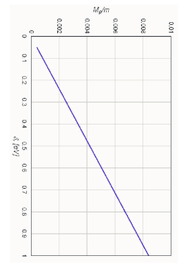
Figure 1: The dependence of the mass of polariton $M_{p}$ on $\delta$. The polariton mass $M_{p}$ is represented in the units of electron mass $m$.

The dilute polaritons constructed by excitons in graphene in the presence of the gap and microcavity photons when gapped graphene is embedded in an optical microcavity form 2D weakly interacting gas of bosons with the pair short-range repulsion. So the superfluid-normal phase transition in this system is the Kosterlitz-Thouless transition Kosterlitz , and the temperature of this transition $T_{c}$ in a two-dimensional microcavity polariton system is determined by the equation:

$$T_{c}=\frac{\pi\hbar^{2}n_{s}(T_{c})}{2k_{B}M_{p}}\ ,$$ (35)

where $n_{s}(T)$ is the superfluid density of the polariton system in a microcavity as a function of temperature $T$, and $k_{B}$ is Boltzmann constant. We obtain the superfluid density as $n_{s}=n-n_{n}$ by determining the density of the normal component $n_{n}$ when we follow the procedure Abrikosov as a linear response of the total momentum with respect to the external velocity:

$$n_{s}=n-\frac{3\zeta(3)}{2\pi\hbar^{2}}\frac{sk_{B}^{3}T^{3}}{c_{S}^{4}M_{p}}\ ,$$ (36)

where $s=4$ is the spin degeneracy factor.

Substituting Eq. (36) for the density $n_{s}$ of the superfluid component into Eq. (35), we obtain an equation for the Kosterlitz-Thouless transition temperature $T_{c}$. The solution of this equation is

$$T_{c}=\left[\left(1+\sqrt{\frac{32}{27}\left(\frac{M_{p}k_{B}T_{c}^{0}}{\pi\hbar^{2}n}\right)^{3}+1}\right)^{1/3}-\left(\sqrt{\frac{32}{27}\left(\frac{M_{p}k_{B}T_{c}^{0}}{\pi\hbar^{2}n}\right)^{3}+1}-1\right)^{1/3}\right]\frac{T_{c}^{0}}{2^{1/3}}\ ,$$ (37)

where $T_{c}^{0}$ is the temperature at which the superfluid density vanishes in the mean-field approximation (i.e., $n_{s}(T_{c}^{0})=0$),

$$T_{c}^{0}=\frac{1}{k_{B}}\left(\frac{\pi\hbar^{2}nc_{s}^{4}M_{p}}{6s\zeta(3)}\right)^{1/3}\ .$$ (38)

The Kosterlitz-Thouless transition temperature $T_{c}$ as a function of $\delta$ and the polariton density $n$ is presented in Fig. 2. It can be seen that $T_{c}$ increases, when $\delta$ decreases and the polariton density $n$ increases. Fig. 3 presents the Kosterlitz-Thouless transition temperature $T_{c}$ as a function of $\delta$ at the different fixed polariton densities $n$. According to Fig. 3, at the same polariton density $n$, $T_{c}$ decreases when $\delta$ increases, and at the same $\delta$, and $T_{c}$ is higher for higher $n$.

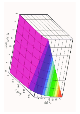
Figure 2: The dependence of the Kosterlitz-Thouless transition temperature $T_{c}$ on $\delta$ and the polariton density $n$.

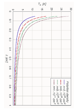
Figure 3: The dependence of the Kosterlitz-Thouless transition temperature $T_{c}$ on $\delta$.

VII Discussion

According to Eq. (33), the effective polariton mass $M_{p}$ is mostly determined by the size of the microcavity, which depends on the gap $\delta$ according to Eq. (20) when the exciton and microcavity photon branches of the spectrum are in resonance at zero momentum. The effective polariton mass $M_{p}$ is proportional to the gap $\delta$. The dependence of the superfluid density $n_{s}$ on the gap $\delta$ is determined also by dependence of the sound velocity $c_{S}$ on the exciton radius $\rho$ ($c_{S}\sim\rho^{1/2}$). Since $\rho\sim\delta^{-1}$, we have $c_{S}\sim\delta^{-1/2}$, and the normal component density $n_{n}\sim\delta^{2}$ according to Eq. (36). The gap dependence of the sound velocity is caused by the gap dependence of exciton-exciton interaction described in Sec. III.2. Therefore, we conclude that the superfluid density $n_{s}$ and Kosterlitz-Thouless temperature $T_{c}$ are decreasing functions of the gap $\delta$ in graphene and increasing functions of the exciton density $n$. Besides, it follows from Eq. (28), that Rabi splitting is decreasing function of the gap as $\hbar\Omega_{R}\sim\delta^{-1/2}$.

The advantage of observing the superfluidity and BEC of polaritons formed by gapped graphene excitons and microcavity photons in comparison with these formed by quantum well excitons and microcavity photons is based on the fact that the superfluidity and BEC of polaritons formed by gapped graphene excitons can be controlled by the gap which depends on doping. The Rabi splitting related to the creation of an exciton in a graphene layer also can controlled by the doping dependent gap.

In conclusion, we propose the superfluidity of 2D exciton polaritons formed by the gapped graphene excitons and microcavity photons, when the gapped graphene layer is embedded in an optical microcavity. The effective exciton polariton mass is calculated as a function of the gap energy in the graphene layers. We demonstrate the effective exciton polariton mass increases when the gap increases and it is directly proportional to $\delta$. We show that the superfluid density $n_{s}$ and the Kosterlitz-Thouless temperature $T_{c}$ increases with the rise of the excitonic density $n$ and decreases with the rise of the gap due to $\delta$ dependence of the sound velocity of collective excitations ($c_{S}\sim\delta^{-1}$), and therefore, could be controlled by $n$ and $\delta$. We demonstrate that the Rabi splitting related to the creation of an exciton in a graphene layer also depends on the gap energy.

Appendix A The eigenfunctions and eigenenergies of an electron in graphene in the presence of gap

We consider two fermions and ignore their interaction (i.e. $V(r)=0$). The electrons in the conduction band, described by the spinor wave function $\psi_{cE}(x,y)$, and the holes in the valence band, described by the spinor wave function $\psi_{vE^{\prime}}(x,y)$, are solutions of the eigenvalue equations

$$H_{-\delta}\psi_{cE}=E\psi_{cE}\ ,\ \ \ H_{\delta}\psi_{vE^{\prime}}=-E^{\prime}\psi_{vE^{\prime}}$$ (39)

of the Dirac-Weyl Hamiltonian

$$H_{\delta}=\left(\begin{matrix}\delta&\hbar v_{F}(\partial_{x}-i\partial_{y})\\ \hbar v_{F}(\partial_{x}+i\partial_{y})&-\delta\\ &\end{matrix}\right)\ .$$ (40)

In the presence of a gap $2\delta$, these solutions are

$$\psi_{cE}(x,y)=\sqrt{\frac{\delta-E}{2E}}\frac{\exp\left(i\left(q_{x}x+q_{y}y\right)\right)}{\sqrt{L_{x}L_{y}}}\left(\begin{array}[]{c}\frac{\hbar v_{F}\left(q_{x}-iq_{y}\right)}{\delta-E}\\ 1\end{array}\right)\ ,$$ (43)

$$\psi_{vE}(x,y)=\sqrt{\frac{\delta+E}{2E}}\frac{\exp\left(i\left(q_{x}x+q_{y}y\right)\right)}{\sqrt{L_{x}L_{y}}}\left(\begin{array}[]{c}\frac{\hbar v_{F}\left(q_{x}-iq_{y}\right)}{\delta+E}\\ 1\end{array}\right)\ ,$$ (46)

where $E=\sqrt{\delta^{2}+\hbar^{2}v_{F}^{2}q^{2}}$ is the energy of the electron or the hole, and $L_{x}$ and $L_{y}$ are lengths in $x$ and $y$ direction, correspondingly. This allows us to construct the four components of the spinor in Eq. (7) from the solutions of Eq. (39) as

$$\phi_{jk}(\mathbf{r}_{1},\mathbf{r}_{2})=\psi_{cE,j}(\mathbf{r}_{1})\psi_{vE^{\prime},k}(\mathbf{r}_{2})\ \ \ (j=a,b;k=a,b)$$ (47)

which solves the eigenvalue equation for two non-interacting particles with the Hamiltonian ${\mathcal{H}}$ in Eq. (8) when $V(r)=0$: ${\mathcal{H}}_{0}\Psi=(E-E^{\prime})\Psi,$ where ${\mathcal{H}}_{0}$ is the Hamiltonian of two non-interacting particles.

Appendix B The representation of polariton operators for the Hamiltonian of the exciton-photon system in a microcavity

We express the exciton and microcavity photon operators in terms of polariton operators. The exciton and photon operators are defined as Ciuti

$$\hat{b}_{\mathbf{P}}=X_{P}\hat{l}_{\mathbf{P}}-C_{P}\hat{u}_{\mathbf{P}}\ ,\hskip 14.22636pt\hat{a}_{\mathbf{P}}=C_{P}\hat{l}_{\mathbf{P}}+X_{P}\hat{u}_{\mathbf{P}}\ ,$$ (48)

where $\hat{l}_{\mathbf{P}}$ and $\hat{u}_{\mathbf{P}}$ are lower and upper polariton Bose operators, respectively, $X_{P}$ and $C_{P}$ are

$$X_{P}=\left(1+\left(\frac{\hbar\Omega_{R}}{\varepsilon_{LP}(P)-\epsilon_{ph}(P)}\right)\right)^{-1/2}\ ,\hskip 14.22636ptC_{P}=-\left(1+\left(\frac{\varepsilon_{LP}(P)-\epsilon_{ph}(P)}{\hbar\Omega_{R}}\right)\right)^{-1/2}\ ,$$ (49)

and the energy dispersion of the low/upper polaritons are

$$\varepsilon_{LP/UP}(P) = \frac{\epsilon_{ph}(P)+\epsilon_{ex}(P)}{2}$$ (50)

$$\mp \frac{1}{2}\sqrt{(\epsilon_{ph}(P)-\epsilon_{ex}(P))^{2}+4|\hbar\Omega_{R}|^{2}}\ .$$

We note that $|X_{P}|^{2}$ and $|C_{P}|^{2}=1-|X_{P}|^{2}$ represent the exciton and cavity photon fractions in the lower polariton.

References

- (1) A. Kavokin and G. Malpeuch, Cavity Polaritons (Elsevier, 2003).
- (2) Physica Status Solidi B 242, 1 (2005), special issue of Physics of Semiconductor Microcavities, edited by B. Deveaud.
- (3) P. Littlewood, Science 316, 989 (2007).
- (4) D. W. Snoke, Solid State Physics. Essential Concepts. (Addison-Wesley, 2008).
- (5) A. H. Castro Neto, F. Guinea, N. M. R. Peres, K. S. Novoselov, and A. K. Geim, Rev. Mod. Phys. 81, 109 (2009).
- (6) S. Das Sarma, S. Adam, E. H. Hwang, and E. Rossi, Rev. Mod. Phys. 83, 407 (2011).
- (7) A. Iyengar, J. Wang, H. A. Fertig, and L. Brey, Phys. Rev. B75, 125430 (2007).
- (8) D. A. Abanin, A. V. Shytov, and L. S. Levitov, Phys. Rev. Lett. 105, 086802 (2010).
- (9) K. F. Mak, J. Shan, and T. F. Heinz, Phys. Rev. Lett. 106, 046401 (2011).
- (10) Yu. E. Lozovik and A. A. Sokolik, JETP Lett. 87, 55 (2008).
- (11) C.-H. Zhang and Y. N. Joglekar, Phys. Rev. B77, 233405 (2008).
- (12) H. Min, R. Bistritzer, J.-J. Su, and A. H. MacDonald, Phys. Rev. B78, 121401(R) (2008).
- (13) R. Bistritzer and A. H. MacDonald, Phys. Rev. Lett. 101, 256406 (2008).
- (14) M. Yu. Kharitonov and K. B. Efetov, Phys. Rev. B78, 241401(R) (2008).
- (15) L. Yang, M. L. Cohen, and S. G. Louie, Nano Lett. 7, 3112 (2007).
- (16) L. Yang, M. L. Cohen, and S. G. Louie, Phys. Rev. Lett. 101, 186401 (2008).
- (17) L. Yang, J. Deslippe, C.-H. Park, M. L. Cohen, and S. G. Louie, Phys. Rev. Lett. 103, 186802 (2009).
- (18) Y. Zhang, T.-T. Tang, C. Girit, Z. Hao, M. C. Martin, A. Zettl, M. F. Crommie, Y. Shen, and F. Wang Nature 459, 820 (2009).
- (19) C.-H. Park and S. G. Louie, Nano Lett. 10, 426 (2010).
- (20) D. Haberer, D. V. Vyalikh, S. Taioli, B. Dora, M. Farjam, J. Fink, D. Marchenko, T. Pichler, K. Ziegler, S. Simonucci, M. S. Dresselhaus, M. Knupfer, B. Büchner, and A. Grüneis, Nano Letters 10, 3360 (2010).
- (21) O. L. Berman, R. Ya. Kezerashvili, and K. Ziegler, Phys. Rev. B85, 035418 (2012).
- (22) O. L. Berman, R. Ya. Kezerashvili, and Yu. E. Lozovik, Phys. Rev. B80, 115302 (2009).
- (23) I. V. Lerner and Yu. E. Lozovik, Sov. Phys. JETP 51, 588 (1980); 53, 763 (1981); A. B. Dzyubenko and Yu. E. Lozovik, J. Phys. A 24, 415 (1991).
- (24) S. Pau, G. Björk, J. Jacobson, H. Cao and Y. Yamamoto, Phys. Rev. B51, 14437 (1995).
- (25) C. Ciuti, P. Schwendimann, and A. Quattropani, Semicond. Sci. Technol. 18 S279 (2003).
- (26) V. Lukose, R. Shankar, and G. Baskaran, Phys. Rev. Lett. 98, 116802 (2007).
- (27) C. Ciuti, V. Savona, C. Piermarocchi, A. Quattropani, and P. Schwendimann, Phys. Rev. B58, 7926 (1998).
- (28) S. Ben-Tabou de-Leon and B. Laikhtman, Phys. Rev. B63, 125306 (2001).
- (29) G. Rochat, C. Ciuti, V. Savona, C. Piermarocchi, A. Quattropani, and P. Schwendimann, Phys. Rev. B61, 13856 (2000).
- (30) B. Laikhtman, Europhys. Lett. 43, 53 (1998).
- (31) A. A. Abrikosov, L. P. Gorkov and I. E. Dzyaloshinski, Methods of Quantum Field Theory in Statistical Physics (Prentice-Hall, Englewood Cliffs. N.J., 1963).
- (32) A. Griffin, Excitations in a Bose-Condensed Liquid (Cambridge University Press, Cambridge, England, 1993).
- (33) J. M. Kosterlitz and D. J. Thouless, J. Phys. C 6, 1181 (1973); D. R. Nelson and J. M. Kosterlitz, Phys. Rev. Lett. 39, 1201 (1977).