Orbit-based dynamical models of the Sculptor dSph galaxy
Abstract
We have developed spherically symmetric dynamical models of dwarf spheroidal galaxies using Schwarzschild’s orbit superposition method. This type of modelling yields constraints both on the total mass distribution (e.g. enclosed mass and scale radius) as well as on the orbital structure of the system (e.g. velocity anisotropy). This method is thus less prone to biases introduced by assumptions in comparison to the more commonly used Jeans modelling, and it allows us to derive the dark matter content in a robust way. Here we present our results for the Sculptor dwarf spheroidal galaxy, after testing our methods on mock data sets. We fit both the second and fourth velocity moment profile to break the mass-anisotropy degeneracy. For an NFW dark matter halo profile, we find that the mass of Sculptor within 1 kpc is , and that its velocity anisotropy profile is tangentially biased and nearly constant with radius. The preferred concentration () is low for its dark matter mass but consistent within the scatter found in N-body cosmological simulations. When we let the value of the central logarithmic slope vary, we find that the best-fit model has , although an NFW cusp or shallower is consistent at 1 confidence level. On the other hand, very cuspy density profiles with logarithmic central slopes are strongly disfavoured for Sculptor.
keywords:
galaxies: dwarf – galaxies: kinematics and dynamics1 Introduction
The existence of dark matter has been invoked to explain discrepancies in the observed kinematics of (systems of) galaxies. Especially in the last 30 years it has become a key ingredient of our current cosmological model, the cold dark matter paradigm (hereafter CDM). N-body simulations have made clear predictions on how dark matter should be distributed in the Universe. Navarro, Frenk & White (1996) showed that simulated dark halos have a universal internal density distribution, now known as the NFW profile. Although there have been some revisions, the general form has remained, and the inner regions of simulated dark halos are found to be cusped with logarithmic slopes in the range to (Navarro et al., 2010). CDM simulations have also revealed the existence of a universal spin distribution and of relations between the characteristic parameters of a dark halo such as concentration and mass (e.g Bullock et al., 2001).
The predictions of the CDM model may be tested using kinematic data. Cleaner tests are generally obtained using tracers located at large distances, i.e. in the regions that are dominated by the dark matter (e.g Romanowsky et al., 2003; Battaglia et al., 2005, 2006; Xue et al., 2008). In these examples, a relatively accurate measurement of the mass contained within a given radius can be obtained, but constraints on the density profile depend on good knowledge of the spatial distribution of the tracers, which may be somewhat uncertain. Another possibility is to use galaxies that are dark matter dominated at all radii, such as low surface brightness systems (de Blok, 2010).
An example of the latter class are the dwarf spheroidal (dSph) galaxies satellites of the Milky Way (Mateo, 1998). These appear to be the most dark matter dominated galaxies with total dynamical mass to stellar light ratios in the order of 100-1000 derived under the assumption of dynamical equilibrium (e.g. Wolf et al., 2010). The nearby dSph galaxies have the additional advantage that individual stars can be resolved, and their red giant branch (RGB) stars are bright enough to measure line-of-sight velocities with errors of a few km s-1 (Mateo et al., 1991). The dynamical modelling of these objects is relatively simple since they are rather round, pressure supported and show little or no rotation. Their high dynamical mass-to-light ratios makes these systems ideal to study dark matter halos, especially their internal structure and to constrain their inner density profiles.
Most of the Milky Way dSph satellites have been modelled using the spherical Jeans equations (e.g. Kleyna et al., 2001; Battaglia et al., 2008; Strigari et al., 2008; Łokas, 2009; Walker et al., 2009), while for more distant objects, such as the dSph satellites of M31, masses have been derived from the average velocity dispersion and projected mass estimators (Kalirai et al., 2010; Collins et al., 2010). In Jeans models one has to specify (i) the form of the light distribution, (ii) the density profile (or equivalently the gravitational potential) of the dark matter component, and (iii) velocity anisotropy of the stars. These characterise a given Jeans model, from which the second velocity moment projected along the line-of-sight can be computed. This is then compared to the measured line-of-sight velocity dispersion of the stars at different locations across the galaxy to establish the performance and characteristic parameters of the specific model.
Jeans modelling suffers from a number of limitations. Firstly the functional form of the velocity anisotropy has to be specified a priori while it is generally unknown. This is because precise measurements of the proper motions of stars in dSph are well beyond reach with current instrumentation. Also inherent to the method is the comparison between the moments of the model to those of the data which requires binning of the data and generally implies loss of information. It is also important to note that there is no guarantee that the resulting distribution function is non-negative everywhere, a requirement for it to be physical. Nonetheless, there have been interesting discoveries based the use of the Jeans equations and which are robust to assumptions of the underlying anisotropy profile. These include for example, the existence of a possible common mass scale of dwarf spheroidals (e.g. Strigari et al., 2008), and the tight constraints on the total mass within the half-light radius of these systems (Walker et al., 2010; Wolf et al., 2010).
Recently, An & Evans (2009) demonstrated that if the tracer population is supported by a spherical dark halo with a core or a cusp (less steep than a singular isothermal sphere), then the central value of the logarithmic slope of the light profile and the central velocity anisotropy are related as . This is valid if , i.e. only if the stars are not dynamically cold in this region. This would imply that the derived existence of a cusp or core at the centre could merely be a consequence of the assumptions alone, if just the second velocity moment is modelled using Jeans equations (see also Ciotti & Morganti, 2010, who show that a density slope-anisotropy inequality holds at all radii, at least for a specific class of distribution functions for spherical systems). Thus care is required in interpreting the outcome of this type of models.
The above discussions shows clearly that there is a need to go beyond the modelling of the second moment using Jeans equations. For example, Łokas (2002) proposed to use higher moments to constrain the internal dynamics of dSphs since the kurtosis profile depends mostly on anisotropy while the velocity dispersion depends both on mass and anisotropy Łokas et al. (2005), hence this lifts some of the degeneracies. Other possibilities would be to use parametrised phase-space distribution functions as pioneered by Kleyna et al. (2001, 2002); Wilkinson et al. (2002a) (see also Amorisco & Evans, 2012a), or the made-to-measure technique (Syer & Tremaine, 1996; Long & Mao, 2010).
In this paper we take a different approach and use Schwarzschild modelling (Schwarzschild, 1979) to probe the internal dynamics and characterise the dark matter content of the Sculptor dwarf spheroidal galaxy. The basic steps of the Schwarzschild method are to integrate a set of orbits in a given potential, calculate the predicted observables for each orbit, and then to weigh the orbits (with non-negative weights) to obtain a model that fits the observed data well in a sense. This approach guarantees that the distribution function (which is reflected in the orbit weights) is non-negative. This method was originally used by Schwarzschild (1979) to prove that a self consistent solution in dynamic equilibrium exists for a triaxial system, but was only implemented to reproduce the density distribution. The method was later extended to include kinematic constrains (Richstone & Tremaine, 1984; Pfenniger, 1984). Since then many codes have been developed (e.g. Richstone & Tremaine, 1984; Rix et al., 1997; van der Marel et al., 1998; Cretton et al., 1999; Valluri et al., 2004; van den Bosch et al., 2008). While first only the lowest moments of the line of sight velocity distribution (mean velocity and velocity dispersion) were fitted, better data have led to the inclusion of higher moments in the fits. While the use of moments allows one to use linear or quadratic programming to find the orbit weights, also likelihood methods using discrete data have been developed (e.g. Merritt & Tremblay, 1993; Wu & Tremaine, 2006; Chanamé et al., 2008). A great advantage of Schwarzschild modelling is that it does not require the specification of the anisotropy profile, this is in fact an outcome of the model (see also Jardel & Gebhardt, 2012; Jardel et al., 2012, for applications on the Fornax and Draco dwarf galaxies).
Sculptor (Scl) is a dwarf spheroidal galaxy satellite of the Milky Way. It lies at high galactic latitude and is located at a heliocentric distance of 79 kpc. With an ellipticity of 0.32 (axis ratio is 0.68) it is not extremely flattened (Irwin & Hatzidimitriou, 1995), allowing us to approximate and model Sculptor as a spherical object. Its luminosity is and one recent estimate of its dynamical mass is within 1.8 kpc (Battaglia et al., 2008). Its (stellar) mass distribution can be well fitted with a Plummer profile with scale radius arcmin ( kpc, Battaglia, 2007). Two large kinematic data sets have been compiled by Battaglia et al. (2008) and by Walker et al. (2009), leading to a total member stars with radial velocity measurements with errors of km/s. As we show below, the combination of these two data sets together with the Schwarzschild method allows us to constrain the dark matter distribution of Sculptor and its internal orbital structure.
This paper is organised as follows. In §2 we will describe the basic ingredients of Schwarzschild modelling, especially focusing on how it can be applied to dSph data. In §3 we validate our model on a mock data set motivated by the current Sculptor data. In §4 we apply the technique to Scl data, we present a brief discussion in §5, and leave our conclusions to §6.
2 Dynamical model
In this section we review some of the theory that provides the basis for our Schwarzschild method. We then describe how to generate models and focus later on how these can be fit to the observables.
2.1 Generalities
The phase-space structure of a galaxy can be specified by its distribution function (hereafter df) , where and are the position and velocity coordinates respectively. The probability of finding a star in the volume is given by . All observables may be derived from knowledge of the df. For example the normalised surface density:
| (1) |
where is the direction along the line-of-sight.
According to the (strong) Jeans (1915) theorem, the df of a steady-state stellar system in which almost all orbits are regular, is a function of the isolating integrals of motion (see also Binney & Tremaine, 2008). Spherically symmetric systems (both in the tracer’s density and the underlying potential) have only regular orbits and generally respect 4 integrals of motion, the energy and the 3 components of the angular momentum vector. However, if the galaxy shows no rotation, due to symmetry, the df will depend only on the energy and the length of the angular momentum vector, i.e. . Furthermore if the velocity distribution is isotropic, the df can only depend on energy and .
Most dSph galaxies are so distant that the only phase-space coordinates that may be measured currently are the projected stellar positions on the sky, and the line-of-sight velocities of (a subset of) its stars. These can be used to derive the surface density and the moments of the line-of-sight velocity distribution:
| (2) | |||||
| (3) | |||||
| (4) |
Here is the projected distance on the sky from the centre of the galaxy and the velocity along the line-of-sight, after subtraction of the centre of mass mean motion.
The above equations suggest that through comparison to the observables it should be possible to derive the form of the df. In some cases, it may be better to parametrise the df and try to estimate its characteristic parameters by comparison to the data (Wilkinson et al., 2002b; Amorisco & Evans, 2012a). However, in this work we prefer to use a non-parametric approach such as the Schwarzschild method. This method uses orbits integrated in a specific gravitational potential as building blocks. From these, light and kinematical profiles may be derived and compared to observations through appropriate weighing of the orbits.
In the case of a dwarf galaxy embedded in a spherical dark matter halo, the gravitational potential can be characterised by a few parameters such as: i) the (enclosed) mass of the dark matter halo , and ii) its scale parameter . Due to the high dynamical mass-to-light ratios of dSphs, we do not expect the stellar mass to have a significant influence on the dynamics of the galaxy. We assume a fixed stellar mass-to-light ratio of as in Walker et al. (2007), and hence from the light distribution we may directly derive the gravitational potential associated to the stars. In the remainder of the paper we shall refer to properties related to the stellar mass and luminosity interchangeably.
Thus in practise, for a given set of parameters of the potential, we integrate orbits and match these to the observations by adjusting the orbital weights. We then repeat this exercise for other values of these parameters. This can be used to establish the values of the set of parameters which result in a better fit to the observables.
2.2 From the model to the observables
Our Schwarzschild method is based on many of the ideas of Rix et al. (1997) and van den Bosch et al. (2008). It is however, a new implementation that is optimised for spherical symmetry. Among other small improvements, our code can be run in parallel and is therefore significantly faster; furthermore for each orbit, we do not store the full line-of-sight velocity distribution but only its moments, which also reduces the computational load.
We now focus on how to generate the observables, namely the surface density and moments of the line-of-sight velocity distribution of the models and how to compare these to data.
For convenience we define the relative angular momentum (where is the angular momentum of a circular orbit of energy ), such that . This enables us to define a rectangular grid in energy and relative angular momentum. Since the Schwarzschild method is based on orbit integrations, the df may be seen as a sum of Dirac delta functions:
| (5) |
where and .
To define the grid in energy and (relative) angular momentum we proceed as follows. For the energy we choose radii between a minimum and maximum radius spaced logarithmically, and take the corresponding energy of a purely radial orbit. The minimum and maximum radii we consider are 0.033 kpc and 24.492 kpc, respectively. For each energy we choose relative angular momenta spaced linearly between and . All orbits are integrated starting from their apocentre.
We also define radial bins on the sky, defined by radii at the edges (). The borders are determined by the kinematic data, by requiring for instance that each bin contains a particular number of stars.
In general, it is convenient to work with the (normalised) mass in a given radial bin:
| (6) |
Thus the mass contributed by orbit of energy and relative angular momentum in the radial bin is:
| (7) |
In the Schwarzschild method this quantity is obtained by integrating the orbit and calculating the fractional time this orbit spends in radial bin . Since we integrate the orbit with a fixed time step, this is simply equivalent to counting the number of times the orbit crosses bin , divided by the number of time steps. To reflect the spherical symmetry, at each time step the position and velocities are rotated randomly times, as in Rix et al. (1997, Eq. 2). Each orbit is integrated for 100 orbital timescales , with , and where is the apocentre radius and the circular velocity at . Each orbit is stored at 1000 points (separated by a constant time step). Therefore the total mass (contributed by all orbits) in bin is:
| (8) |
where is the density of states. The coefficients are known as the orbital weights.
We may now proceed to calculate the light-weighted second and fourth moments of the line-of-sight velocity distribution in a given projected radial bin as:
| (9) | |||||
| (10) |
where and are the second and fourth moment respectively of orbit . The integral is also derived from the orbit integrations. However, instead of counting each time the orbit is found in bin , we add the corresponding second moment in quadrature (and to the fourth power for the fourth moment) and at the end divide by the number of time steps. Note that the moments are linear in the orbital weights, which allows us to find a solution using quadratic programming, while for instance the kurtosis () is not.
It is possible to consider the orbit weights () as free parameters whose exact values will be determined through comparison to the observables. However this would imply that the number of orbits that are integrated to reproduce the observables is exactly equal to the number of free parameters that define the df. Decoupling these two sets of quantities is clearly desirable, see e.g. Cretton et al. (1999). This procedure is known as dithering and results in smoother density distributions while keeping the number of free parameters in the distribution function small.
While we may use orbits to reproduce the observables, we choose only free parameters to characterise the distribution function, where we take . The coefficients of the distribution function are related to the orbit weights () as follows:
| (11) |
where indicates the integer part, e.g. . Therefore orbits share the same df coefficient. In practice, one can simply average the quantities obtained from the individual orbits. We choose and , which results in free parameters for the distribution function, but we integrate orbits.
To fit models to the data we generally use projected quantities (i.e. the observables). However, if one knows (or has derived) the df coefficients, it is also possible to make predictions for quantities that are not (yet) directly observable, such as the intrinsic (3d) density distribution or moments of the full velocity distribution. For example, the mass contained in the (spherical) radial bin contributed by orbit is
| (12) |
where the integral is computed from the orbital integrations, and is the radial density profile of orbit . In practise we use (3d) radial bins, spaced linearly between kpc and kpc. Similarly we also store the radial and tangential velocity dispersions in these bins. Although we do not store the intrinsic properties beyond 1.5 kpc, this has no effect on the way the projected properties are determined. Note that the intrinsic properties are not used in any of the fitting routines but may be used for inferring for instance the intrinsic velocity anisotropy profile.
Orbits are integrated using the GNU Scientific Library (GSL) ordinary differential equation solver using an 8th order (Runge Kutta) Prince-Dormand method. We found that the energy is conserved to better than 0.1%.
2.3 Fitting procedure
2.3.1 Light distribution
Our first requirement is for the model to fit the observed light distribution. We assume that this is known accurately. We require that the projected mass (or light) in each bin is matched within 1 per cent. Given our assumption of a constant stellar mass-to-light ratio, we make no distinction between surface brightness and stellar mass surface density in what follows. From the assumed brightness profile , we calculate:
| (13) |
and thus require for each projected radial bin that:
| (14) |
Note that the number of bins for the light does not have to equal the number of bins for the kinematics, in this work we choose 250 bins for fitting the light distribution.
2.3.2 Kinematics
To derive the line-of-sight velocity dispersion profile we calculate the second and fourth moment estimators of the line-of-sight velocity distribution and in bins containing at least stars. Assuming that the measurement errors are normally distributed, and all measurements and errors are independent and uncorrelated, we can obtain of the population as follows. The expectation value of the second moment is
| (15) |
where is the unknown noise of measurement , which we assume is drawn from a normal distribution with dispersion (i.e. this is the formal error of measurement ). Hence is the average of the estimated squared errors. Here the true value of the second moment. Therefore, our best estimate for the second moment of the underlying population is:
| (16) |
Similarly, the expectation value of the fourth moment
| (17) |
where we have used that the fourth moment of a normal distribution is 3. Therefore our estimate for the fourth moment is:
| (18) |
where we have assumed .
The variance of the second moment , can be determined using , which yields
| (19) |
Although we formally need , we have found by testing with a Gaussian distribution, that for our purposes . For the variance of the fourth moment we find:
| (20) | |||||
which require the and moments:
| (21) | |||||
| (22) |
and again we use .
The likelihood of the kinematic data given a model is:
| (23) |
where
| (24) |
Here is given by Eq. (9), is the estimate from the data for bin and similarly for the fourth moment111Here we have neglected correlations between the moments, although these may exist in practice..
2.3.3 Finding a solution
We need to find the that maximise the probability (Eq. 23) or minimise the , under the condition that all are positive (and sum up to unity) and the light distribution is reproduced to within 1 per cent. This problem can easily be solved by quadratic programming (QP), since the minimisation is quadratic in the df coefficients, and the constraints are linear. Note however that for this non-parametric problem, the parameter space is very large, and a solution will often yield an unrealistically spiky df. To effectively reduce the parameter space and yield a smoother df, we add a regularisation constraint, in analogy to Cretton et al. (1999) and van den Bosch et al. (2008), by including a penalty term to the total . This term has the form:
| (25a) | |||
| (25b) | |||
| (25c) |
where and are small for a smooth df. This smoothness requirement is implemented by demanding the second order derivatives of the df to be small, which we compute by taking second order finite differences (Eqs. 25b-25c).
In our case we found to work well, and we calibrate in the next section. The terms are the inverse of the (normalised) masses inside the radii defined by our energy grid (§2.2) (see also van den Bosch et al., 2008, Eq. 29). Since the regularisation term is quadratic in the df coefficients, it can also be optimised using the QP.
The total now becomes:
| (26) |
Minimising this equation, in combination with the linear constrains of the and the linear constraints on the light distribution (Eq. 14) defines the problem for the QP.
3 Testing the method
3.1 Plummer profile embedded in an NFW dark matter halo
3.1.1 Mock Sculptor
We now create a mock galaxy that may be representative of Sculptor according to previously published dynamical models of this system (Battaglia et al., 2008). The goal is to test our method in the region of parameter space where we expect Sculptor to be. For the stellar component we choose a Plummer profile with total mass and a scale radius kpc. The stellar component is embedded in a spherical NFW dark matter halo with scale kpc, and enclosed mass at 1 kpc of . The radial density profile for the NFW halo is of the form . We set the velocity anisotropy to be constant, . Recall that and (where for every ) and are the second moments of the intrinsic velocity distribution at radius in the tangential and radial directions respectively. Note that in this model, although the central velocity dispersion is null222which implies there is no conflict with the An & Evans (2009) theorem., the line-of-sight velocity dispersion is finite, and has a value . By assuming the df to be separable, i.e. , we may compute it explicitly (numerically) as described in Appendix A.
As an extra check that our model galaxy is physical and stable, we have generated phase-space coordinates for stars from its df, and simulated it numerically using GADGET-2 (Springel, 2005). In this simulation the stars are represented as N-bodies and they are embedded in the static potential given by the dark halo of our mock Sculptor model. We found that, even after Gyr of evolution, the density distribution, velocity dispersion profiles and the anisotropy match the initial values well.
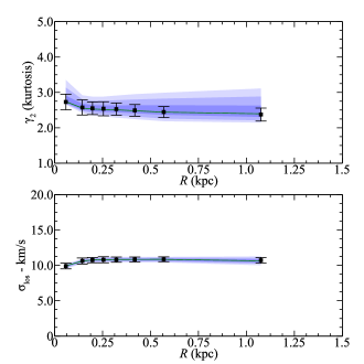
To generate observations of our mock Sculptor we could draw a random sample of stars from its distribution function. However, this has the disadvantage that many realisations would be required to test if the mean of the recovered quantities matches the known input values. Therefore, for the purposes of testing our modelling technique we prefer to compute the moments of the line-of-sight velocity distribution at different radii directly from the known distribution function, as this is less susceptible to randomness. We add uncertainties in the moments and choose the location of the radial bins to match the Sculptor data set. Fig. 1 shows the line of sight velocity dispersion profile and the kurtosis derived in this way. Note however in the model fitting we use the second and fourth moments since these are linear in the df coefficients. We calculate the uncertainties in the moments using Eqs.(19) and (20), assuming no measurement errors since these contribute only of the error budget for the typical measurement errors of 2 and line of sight velocity dispersions of 10 found in dSph. Therefore the uncertainties in the moments are only due to the number of objects per bin. Here we we choose to have 250 stars per bin, which gives a total 8 bins for a sample of 2000 objects.
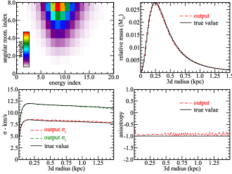
We proceed to test our code in two steps. In the first instance our aim is to establish how well the method recovers the intrinsic properties of our mock galaxy if the df is known. Thus in this first test we use the known df to compute the df coefficients. These define the orbital weights which our Schwarzschild code uses to calculate the observables. The df coefficients are shown in the upper left panel of Fig. 2. The recovered (normalised) mass per intrinsic (3d) bin (Eq. 12), is plotted in the top right panel of the same figure. The red dashed curve shows the output of the Schwarzschild code, while solid black corresponds to the true values. In the lower left panel we plot the velocity dispersions for the radial (red) and tangential (green) directions. The solid curves indicate the true values, whereas in dashed we showed the recovered dispersions. Here the “true” velocity dispersion has been calculated using the Jeans equations (Binney & Tremaine, 2008, chapter 4). The lower right panel shows the true (solid black) and the recovered (dashed red) anisotropy as a function of radius. This exercise shows that given the correct weights we are indeed able to recover the known intrinsic properties of our mock galaxy.
The small deviations from the true values especially visible in the anisotropy profile are expected since the df coefficients only approximate the true df. These deviations can thus be removed by increasing the number of df coefficients. For example, if we double the number of coefficients in the energy and angular momentum directions, the small offset between the true and recovered anisotropy profiles disappears. The increase in the resolution in the energy direction also leads to the elimination of the wiggles in the anisotropy profile. On the other hand, the turnover of the anisotropy profile seen at small radii is related to the sampling of orbits with the highest binding energy. Recall that we sample orbits from a minimum radius kpc, so that the highest binding energy radial orbit has its apocentre at . The orbits that contribute to the region are those which are very elongated with pericentres inside this radius and with large apocentres ( beyond ), and the set of orbits with the highest binding energy but which have more angular momentum. These more circular orbits only contribute within a small range in radii, and hence the resulting velocity ellipsoid is radially biased. Clearly if we were to reduce , i.e. increase the sampling of orbits in the central regions, this will lead to a decrease in the radius at which the velocity anisotropy turns over. However, we deem this unnecessary as the amount of mass associated to this region is negligible, and this regime is in fact outside the reach of observations since we only have access to observables along the line-of-sight, and a star at small projected radius could be located at larger physical radii from the centre. Furthermore, the size of the currently available data sets is a strongly limiting factor (see next paragraph).
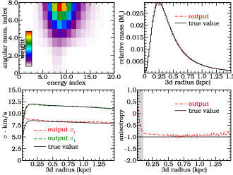
We now use the full Schwarzschild method, and solve for the df using QP. For the regularisation parameters we found to give good results. Fig. 3 summarises our findings. The overall properties of the df are well recovered as well as the remaining characteristics (see Fig. 2 for comparison). The anisotropy is recovered accurately except for 0.1 kpc. This is not due to sampling of highly-bound orbits discussed above, but is mostly driven by the small number of stars in this (3d) inner region. Running the same experiment with a larger data set (10 000 and 50 000 stars) we see the mismatch in the anisotropy to occur at smaller radii. In practise, this means that with the current data sets we are not sensitive to the anisotropy at 0.1 kpc.
3.1.2 Global halo parameter recovery
In the above tests we showed that the Schwarzschild code accurately recovers the df and therefore the kinematic properties of our mock dwarf galaxy. This test was done assuming that the (enclosed) mass within kpc of the NFW halo () and its scale () were known. We now focus on how to estimate these parameters directly.
We proceed to calculate the probability of a model for a set of parameters values. In our case these parameters are and . However, instead of calculating this probability on a regular grid as done in e.g. Gebhardt et al. (2007) and van den Bosch et al. (2008), we use an adaptive method, similar to Gebhardt & Thomas (2009). This first finds the probability density function (pdf) on a coarse grid and then determines where the pdf needs to be refined, and does so hierarchically. This allows us to obtain a relatively smooth pdf via the evaluation of a small number of models. For each set of model parameters we calculate the (relative) probability as (Eq. 24). This results in estimates of the best fit parameters, as well as in confidence intervals. We assume the prior on to be uniform in in the range 333Outside this interval the pdf is essentially zero. and the prior on uniform in in the range .
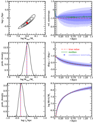
The pdf for the parameters and for our mock Sculptor model is shown in the top left panel of Fig. 4. The pdf is nicely centred on the input values and kpc. The maximum likelihood value (blue dot or lines) almost equals the input value, where the small deviation is caused by the discretisation of the pdf. Although the enclosed mass at 1 kpc is recovered both accurately and precisely (mean , corresponding to a 7% uncertainty, or ), the scale radius is more poorly constrained (mean kpc, corresponding to a 37% uncertainty, or kpc). Note that the marginalised pdf for and are somewhat asymmetric (a reflection of what is seen in the upper left panel of Fig. 4), and this leads to slightly biased mean values for the parameters of the model.
Each Schwarzschild model (i.e. for a given and ) results in a single anisotropy profile. To find the pdf of the velocity anisotropy profile one should integrate (marginalise) over all possible df coefficients (as in Magorrian, 2006). However this is not always feasible due to the high dimensionality of the parameter space required to specify the df ( for this model). Instead we take the single anisotropy profile of each model, and calculate the probability density function for the anisotropy as a function of radius as follows:
| (27) |
We plot the median anisotropy as a function of radius in green in the top right panel of Fig. 4, together with the 68.3, 95.4 and 99.7 percent confidence intervals in blue. Note however, that the anisotropy values at different radii are not independent. The input anisotropy is indicated by the red dashed line. The anisotropy seems to be reproduced quite accurately, except at small radii. Since our technique recovers nearly perfectly the input values of the model, the anisotropy profile found is essentially equivalent to that derived in Fig. 3. The mismatch at small radii is explained in the previous section, and the apparent small uncertainty in the anisotropy in this region may be understood from the following argument. Using the Jeans equation, we may express the mass within a given radius as
where , is the anisotropy, and . For any model without a black hole in the centre, the as . For a cored profile (as we have assumed) in this limit. This implies that there is quite a strong restriction on the behaviour of (and ) at small radii. The above equation implies that as ,
and since as to have a physical solution in a cuspy dark matter halo according to An & Evans (2009), then this means that there is only one possible at , for any model, i.e. value of and .
In the central right panel of Fig. 4 we plot the logarithmic slope () of the dark matter density () as a function of radius:
| (28) |
In the inner parts and in the outer regions due to our choice of the NFW profile. In the next section we also explore a different functional form for the halo density profile, which makes this plot more meaningful and useful for later comparison.
In the bottom right panel we plot the enclosed (dark matter) mass as a function of radius. The least uncertainty in the enclosed mass is at kpc. This radius is close to the half light radius kpc where Walker et al. (2009, 2010) and Wolf et al. (2010) find the enclosed mass to be most robustly determined and to be independent of anisotropy.
The line of sight velocity dispersion and the kurtosis profiles obtained from the models are shown as the blue contours in Fig. 1. These have been computed in an analogous manner to the anisotropy profile, i.e. as in Eq. (27). This figure shows that the resulting curves are in excellent agreement with the input profiles.
To gain further confidence in our methodology, we have also performed a similar set of tests for different anisotropy profiles, while keeping the same stellar and dark matter density profiles. In one case the anisotropy varied from in the centre to at larger radii (i.e. from tangentially to radially biased). The other case we have tested has an anisotropy profile that changes from at the centre to at larger radii (i.e. from radial to tangential anisotropy). Also in these cases all the quantities recovered are in excellent agreement with the input values, indicating that our methodology works well and is robust.
3.2 Changing the dark matter halo density profile
In reality we will not know the actual density profile of the dark matter halo hosting a galaxy like Sculptor, and we would like to determine this from the data. A particularly interesting quantity is the inner slope of the density profile since this depends on the nature of the dark matter particles themselves, i.e. whether it is cold, warm or self-interacting (Avila-Reese et al., 2001; Spergel & Steinhardt, 2000).
Therefore, in this section we use our mock Sculptor, which is embedded in an NFW profile, but we assume a more general functional form to test the performance of our Schwarzschild method, i.e. we take:
| (29) |
such that for this reduces to the NFW case. For the orbit integration we need to know the potential (or rather the forces) generated by this density distribution. Since no general analytic expression exists for these general potentials, we have to solve Poisson’s equation numerically. We do this using the FEM (Finite Element Method) method (e.g. Pepper & Heinrich, 1992). Our basis functions are Lagrange polynomials of degree to (cubic), which leads to a force field of order 2 (quadratic). We use a grid of 200 points in log radius, from kpc. Testing this in the case of the NFW profile we find that the relative errors in the force in this range are .
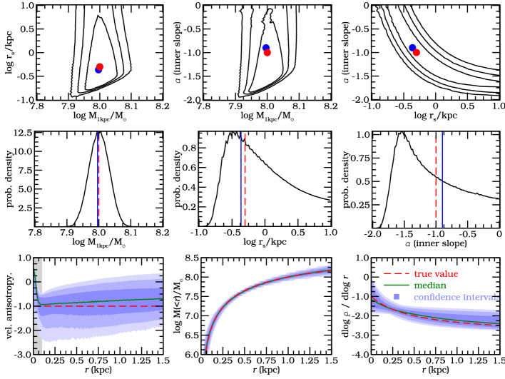
We use our Schwarzschild code to find the best model that fits our mock Sculptor data, now with an additional unknown parameter , assuming a uniform prior in the range ( corresponds to a central hole in the dark matter distribution, which we do not consider). The results are given in Fig. 5. The top row in shows the joint pdfs, marginalised over the remaining parameter. The middle row shows the pdfs of the single parameters, marginalised over the other two parameters. The blue dots and blue lines indicate the maximum likelihood value (of the unmarginalised pdf). In the bottom row the recovered anisotropy, mass and density profile are shown.
In general, all quantities are recovered quite well. However, the pdf of versus shows an important degeneracy between these parameters, indicating that it is hard to determine either of these quantities reliably from our mock data set. The maximum likelihood (the blue dot) is slightly offset from the input value (red dot), which may indicate small systematic errors due to for instance the discretisation of the distribution function. However, note that since this systematic offset is in the direction of the degeneracy, the systematic error is small compared to the statistical uncertainty and therefore we do no consider this to be a problem for data sets of this size and quality. This analysis suggests that the current data is not sufficient to provide a good estimate of the inner slope for these models. The limitation lies in the number of stars with spectroscopic measurements (which in the case tested here is 2000) and/or their spatial distribution.
4 Application to the Sculptor dSph galaxy
4.1 Data and extracted velocity moments
We use the line-of-sight velocities of Battaglia et al. (2008, 1073 stars, hereafter B08)and Walker et al. (2009, 1541 stars, hereafter W09)444Although Amorisco & Evans (2012b) have reported a systematic velocity offset of 1.5 km/s in the dataset of W09 compared to B08’s, we here perform no correction. The various tests we have done show that this offset has no visible effect on the results.. In the case of duplicates (stars in common in the datasets) we average the line-of-sight velocities and the errors (in quadrature). Two observations are considered to be from the same star when the astrometry agrees within 1 arcsec, and a velocity difference less than 3, where is the average velocity error. Inspection of the relative distances between stars in the datasets shows that this criterion is optimal to sieve duplicates. This procedure led to the identification of 308 duplicates, roughly 11% of the combined dataset.
To create a velocity dispersion profile, we first need to convert the measurements of the heliocentric line-of-sight velocities into line-of-sight velocities that take into account the space motion of Sculptor. We provide below a brief summary of this procedure and refer the reader to Appendix B for more details.
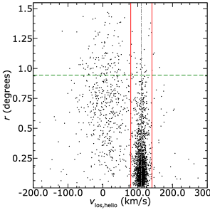
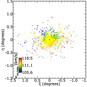
The heliocentric line-of-sight velocities of Sculptor’s stars are shown in Fig. 6. As can be seen from this figure, there appears to be a velocity gradient along the major axis (see also Fig. 1 of B08). The presence of such a gradient could be due to intrinsic rotation in Sculptor, as suggested by B08. On the other hand it is also possible that the gradient is a result of the projection of the proper motion of the centre of mass of Sculptor (or a mix of both), in which case it can be used to infer its space velocity (Walker et al., 2008). In absence of independent and direct measurements of the proper motion of Sculptor, it remains debatable what the source of the gradient is. For simplicity, here we assume that Sculptor does not rotate and we derive the velocity of the centre of mass of Sculptor from the line-of-sight measurements in Appendix B. We note that in practice, our procedure simply removes the gradient, which one might say is equivalent to having removed (solid body) rotation.
4.1.1 Velocity dispersion profile
For our dynamic modelling, we need to calculate the velocity dispersion profile of Sculptor in radial bins. To this end, we initially make a rough selection of the likely members of Sculptor, and then perform a more thorough analysis including the effects of Milky Way contaminants. In the first step, we take the systemic heliocentric radial velocity ( km s-1) and the mean velocity dispersion ( km s-1) from B08. We require that the member stars are within of the systemic velocity of Sculptor, as indicated by the red solid lines in the right panel of Fig. 6. Furthermore we also require that they are located within arcsec ( deg, kpc), indicated by the green dashed line in the same panel. We add this requirement since we are not confident that outside this radius a reliable velocity dispersion can be measured due to the low number density of (probable) Sculptor members compared to Milky Way stars. An improved method for discriminating Milky Way contaminants based on surface gravity in the data set of B08 has been developed by (Battaglia & Starkenburg, 2012), see also Walker et al. (2009).
We then define radial bins such that each but the last bin contains at least 250 stars that match these criteria. From the total of unique (i.e. non-duplicates) 2306 stars, 1695 match the above two criteria, resulting in 7 radial bins, where the last one contains 195 stars.
After we defined our bins to include at least 250 probable members, we remove the requirement of being within of the systemic velocity of Sculptor. We now only require arcsec ( kpc), so all stars below the green dashed line in top panel of Fig. 6 are considered for calculating the velocity dispersions (2153 stars). We now use a model for the velocity distribution of the foreground contamination and of Sculptor itself, which then allows us to calculate the most likely velocity dispersion in each radial bin.
Following B08 and W09 we model the velocity distribution in a radial bin as a sum of Gaussians. The velocity distribution of Sculptor itself is modelled as a single Gaussian, while that of the Milky Way is modelled as a sum of two Gaussians555This gives a good fit to the Besançon model in this region of the sky and for stars with colours and magnitudes in the observed range (Robin et al., 2003)., following B08. Then the probability of the velocity dispersion of Sculptor in radial bin with data is:
| (30) |
where and are the radius and velocity of the star in the bin, is the number of stars in bin , is the prior, which we take flat between the range km s-1 and and indicate the Boolean value of being a member star of Sculptor or not. The proportionality can be used since the denominator is a normalisation constant. The first terms in the last line of Eq. (30) can be expanded further (for each ):
| (31) |
We take the prior on membership, to be equal . Using the model of Sculptor as described above, , the normalised surface density and is a Gaussian convolved with the individual measurement errors on .
The second term in Eq. (30) can similarly be derived by replacing with in Eq. (31), is the density of the Milky Way foreground. Since the normalisation is not important, we only need to know the ratio in each bin666Although the sampling of B08 and W09 is different, we have found in tests that this has no influence on our results. . This can be estimated by the ratio of stars outside the and inside the velocity dispersion. Furthermore, if there is any bias in the sampling of the kinematic data (which usually is the case), it will affect both the Sculptor data and the foreground data in equal ways, and will cancel out in the ratio. The term is the weighted sum of two Gaussians as described in Battaglia et al. (2008).
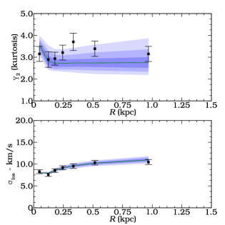
For each radial bin we find the maximum likelihood value for the velocity dispersion. After this, we perform a clipping around the mean, and estimate the second and fourth moments for the remaining stars using Eqs. (16) and (18). The errors are computed from Eqs. (19) and (20). The final sample contains 1696 member stars. Fig. 7 shows the resulting velocity dispersion profile and the kurtosis (). The line-of-sight velocity dispersion is well-constrained, it is relatively flat although it appears to be slightly rising with radius. The kurtosis has larger error bars, and this implies that additional modelling is required to establish in a robust statistical way what the shape of the velocity ellipsoid is (Gerhard, 1993).
4.2 Schwarzschild method applied to Sculptor
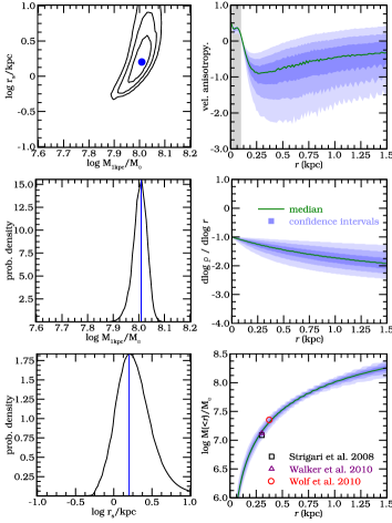
We now apply the Schwarzschild method to the data from the Sculptor dSph and model this galaxy as a (non-rotating) spherically symmetric system. For the light distribution we assume a Plummer profile with scale radius kpc (Battaglia 2007).
We first assume that Sculptor is embedded in an NFW dark matter halo, as we did for mock Sculptor in §3.1. The results of this modelling are shown in Fig. 8. We obtain a tight constraint on the enclosed dark matter mass of (7% uncertainty, or ). The scale radius at kpc (76% uncertainty, or kpc) is less well constrained, similar to what we find for mock Sculptor. In comparison to our mock model, the Sculptor dwarf galaxy would seem to have a larger scale radius (see Fig. 4).
Our estimates are consistent with those derived in previous work for the NFW family of mass models. For example, Walker et al. (2009, 2010) derive a mass of within 1.1 kpc, while we estimate within the same distance with smaller error bars. On the other hand, Battaglia et al. (2008) obtained a mass of within 1.8 kpc, while our measurement at this radius is . The mass estimates by Strigari et al. (2008) Walker et al. (2010, MCMC value) and Wolf et al. (2010) are over plotted in the bottom right panel of Fig. 8, and all three agree very well with ours and are within the confidence regions.
The top right panel of Fig. 8 shows that Sculptor’s anisotropy is mostly tangential and fairly constant with radius, except near the centre where it becomes slightly more isotropic (even after talking into account our limitations due to the projection effects shown and discussed in the context of Fig. 3). This anisotropy profile at kpc is consistent with the constant anisotropy assumed in Jeans models of Sculptor, as by Walker et al. (2007), who find .
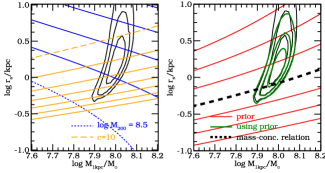
We plot the joint pdf of and again in Fig. 9. In the left panel we plot lines of constant virial mass in blue777 is the virial mass (mass enclosed within ), where is the distance at which the average density of a dark matter halo is 200 times the cosmological density (e.g. Binney & Tremaine, 2008, §2.2)., with the blue dotted line indicating a value of , increasing with steps of dex until . Orange lines indicate constant concentration values, with the orange dashed line corresponding to , increasing with steps of until . This shows that the concentration of Sculptor is and that the virial mass is not well determined (not better than within factor of 100 at a 3 level uncertainty).
Cosmological N-body simulations of dark matter have shown that there is a relation between the concentration of dark matter halos and their virial masses, the so called mass-concentration relation (e.g. Bullock et al., 2001). In the right panel of the Fig. 9, we show as the dashed black line the mass-concentration relation of Macciò et al. (2007):
| (32) |
Judging solely from this relationship this would suggest that Sculptor is not compatible with the current CDM cosmology. If we however plot the intrinsic scatter of in the same panel (solid red lines, 1,2 and 3 contours) we see that Sculptor lies well within the 1 and 2 contours. We can also use the mass-concentration relation as a prior in our models. The results are shown as the green contours in this figure and they are slightly smaller than the original contours. The effect is small, but leads to a narrowing down of the possible values for .
4.3 Dark matter inner density profile
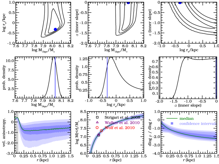
We now consider a more general dark matter profile for the dark matter halo of Sculptor as we did for our mock models in §3.2 by allowing in the inner slope to vary (see Eq. 29). The results are shown in Fig. 10.
This figure shows that the maximum likelihood value for and that the velocity anisotropy recovered by the Schwarzschild method are in very good agreement with the values obtained when is fixed to as in Fig. 8. However, as discussed in Sec. 3.2 the strong degeneracy between and implies that the scale radius is less well determined.
The middle right panel of Fig. 10 shows that the distribution of values for the inner slope is very broad. Nonetheless it is clear that very steep cuspy profiles () are excluded. The maximum likelihood value is reached for a cored profile (), although this is statistically indistinguishable from slightly cuspier slopes as evidenced by the pdfs in this Figure. The bottom right panel of Fig. 10 shows that at a distance of 250 pc (where the anisotropy profile begins to change its shape, and which according to our tests in Sec. 3.2 is the inner most point where it is reliably determined) the median logarithmic slope profile (green line) takes a value of , which is larger that found in our mock Sculptor model (). Since the maximum likelihood value of estimated by the Schwarzschild method is not very different from that assumed in mock Sculptor, this comparison would suggest that the density profile of Sculptor is shallower than NFW, although the uncertainties are still too large to make a very firm statement.
5 Discussion
Our results agree with previous studies of Sculptor that a central logarithmic slope is more likely than the NFW cusp (Battaglia et al., 2008; Walker & Peñarrubia, 2011; Amorisco & Evans, 2012a; Agnello & Evans, 2012), although in our case the evidence is clearly not strong enough to rule out the latter. Note however, that many, though not all, of these works have tested the presence of a true core, namely and not just at the centre. A comparison of the statistical significance of our results with Walker & Peñarrubia (2011) or Agnello & Evans (2012) is not straightforward because of the very different methods employed to estimate the inner slope. These authors use the existence of two distinct populations (metal-rich and metal-poor) to constrain the mass distribution (which is modelled non-parametrically), and this may or may not be the cause of the difference. Amorisco & Evans (2012a) favour a cored profile over an NFW with a high significance, but their conclusion is based on the assumption that two populations follow Michie-King phase-space distribution functions, which are radially anisotropic. In Amorisco & Evans (2012b) these authors present evidence that the velocity anisotropy of Sculptor might in fact radial. This is in conflict with our results, since we find, with high confidence levels, that the orbits of stars in Sculptor are tangentially biased (also when marginalised over all models), especially at radii beyond 250 pc, where the dominant population is the metal-poor one. Furthermore, also Walker et al. (2007); Battaglia et al. (2008) and Łokas (2009) favour a tangentially biased constant anisotropy profile in their Jeans models of this system.
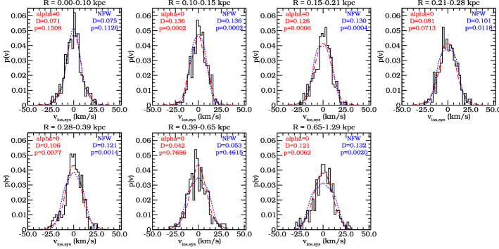
Given these seemingly contradictory results, it is worthwhile taking a closer look at the line-of-sight velocity distributions to understand where the discrepancies might arise. Figure 11 shows these distributions (black histograms) together with the results obtained for the best fit NFW (blue dotted) and (red dashed) models. This figure shows that the l.o.s. velocity distribution is more peaked at small radii than in the outskirts, where it is more flat-topped. This is consistent with our measurements of the l.o.s. kurtosis, and also with our derived anisotropy profile. As shown by Dejonghe (1987), systems with a tangentially biased velocity ellipsoid have a flat-topped l.o.s. velocity distribution only at large radii, while in the centre, this distribution is always more peaked. This is because the l.o.s. towards the centre has contributions from stars located at a larger range of radii, and hence also from radial plunging orbits, which drives the shape of the projected velocity distribution to be more peaked. This is known as the “complementarity property”, and the results of our modeling would be consistent with such a scenario.
Figure 11 also shows the small differences between the and profiles, and lend support to our conclusion that the two profiles are both relatively good representations of the data. This is quantified by a KS-test, whose probabilities are indicated in the corners of each of the panels of this figure. In a few of the radial bins, none of the models fair particularly well. The model tends to fit better the peak of the histogram, and this could be partly to the lower but still tangential anisotropy since for most radii.
The question thus arises as why do Amorisco & Evans (2012b) find a radial anisotropy. Just like us, these authors have utilized the W09 dataset. However, they use stars with a membership probability of 0.5 (as estimated by W09), and do not model the contamination by the Milky Way any further. In the presence of contaminants, l.o.s. velocity distributions have extended wings, and this produces a peaky distribution akin that of truly radially anisotropic systems. We have tested this idea by measuring the kurtosis for two different membership probability values , as in Amorisco & Evans (2012b), and (which is more in line with our more sophisticated modeling of the foreground), and found a significant difference: the kurtosis is in the first case while in the second case it is consistent with that shown in Fig. 6 of this paper.
In conclusion, care is required when contamination is present, and the differences between profiles that have such as the NFW or , although present, are perhaps not as dramatic as maintained in other published work.
6 Conclusions
We have presented a spherically symmetric dynamical model for the Sculptor dwarf spheroidal galaxy using the Schwarzschild orbit superposition method. This method fits a set of observables, which in our case are the light, the second and fourth moments of the line of sight velocity distribution. We have tested this method on a mock model for the Sculptor dSph galaxy embedded in an NFW profile, and generated with similar sampling and velocity errors as the data currently available for this system.
In our tests we have found our method to give precise ( uncertainty) and accurate estimates for the mass within 1 kpc, when assuming that the underlying gravitational potential is of NFW form. However the scale radius is recovered less precisely ( uncertainty) for data sets containing member stars. We have also explored a more general model for the dark matter halo and found that we are able to measure the logarithmic slope of its density profile, although the central value is weakly constrained. Nonetheless we find that the maximum likelihood value for the inner slope is very close to the input value.
We then used the Schwarzschild method on Sculptor after having estimated the second and fourth line of sight velocity moments for this galaxy. Assuming an NFW profile for the dark matter profile, we derive a mass within 1 kpc of , and find the concentration () to be compatible with current CDM predictions, given the expected scatter in the mass-concentration relation (Macciò et al., 2007). When we try to constrain the inner slope of the dark matter density profile of Sculptor, we can exclude very cuspy profiles (). However, given the current data set, our method does not seem to be able to discriminate in a statistically significant way between a cusp and a central logarithmic slope , although the latter is the most likely value. We are, however, able to determine that the logarithmic slope of the density profile falls off to the value of at a distance of kpc.
The Schwarzschild method is also able to derive the velocity anisotropy profile, except near the centre where we are limited by the number of tracers. For Sculptor we find this to be tangentially biased with a hint that it may become more isotropic for pc. This result is nearly independent of the assumed shape of the dark matter density profile, whether NFW or its generalised form. This nearly flat tangentially anisotropic ellipsoid should hold clues to the formation and dynamical evolution of Sculptor but it is as yet unclear whether a model exists that can reproduce this trend.
Models in which stars follow the dark matter are inconsistent with our results, as they predict a more radially anisotropic velocity ellipsoid (Diemand et al., 2004). On the other hand, the tidal stirring of a disky galaxy (see e.g. Mayer, 2010), can lead to a tangentially biased ellipsoid. However, this model predicts that the ellipsoid becomes increasingly tangential with radius as a consequence also of tidal stripping, and this is not what we derive at face value.
Schwarzschild modelling does not have to assume a parametric form for the velocity anisotropy as for instance in the commonly used Jeans modelling. We therefore believe that we are less affected by biases due to assumptions compared to such class of models. Furthermore, by construction we are guaranteed that our models are physical in the sense of having non-negative distribution functions.
We plan to develop the Schwarzschild method further to work with the full line of sight velocity distribution, instead of binning the data and comparing it the the velocity moments profile. Avoiding the loss of information when binning, we expect that this may give us better estimates for the inner slope and the anisotropy profile. Also, since neither Sculptor nor any of the other dwarf spheroidal galaxies are spherical, we are developing a non spherical orbit-based dynamical model. We also plan to apply this modelling to other dwarf spheroidal galaxies such as Fornax, Carina and Sextans in future work.
Acknowledgements
AH and MB are grateful to NOVA for financial support. AH acknowledges financial support the European Research Council under ERC-Starting Grant GALACTICA-240271. We are also grateful to Carlos Vera-Ciro and Simon White for various interesting discussions.
References
- Agnello & Evans (2012) Agnello A., Evans N. W., 2012, ApJ, 754, L39
- Amorisco & Evans (2012a) Amorisco N. C., Evans N. W., 2012a, MNRAS, 419, 184
- Amorisco & Evans (2012b) Amorisco N. C., Evans N. W., 2012b, MNRAS, 424, 1899
- An & Evans (2009) An J. H., Evans N. W., 2009, ApJ, 701, 1500
- Avila-Reese et al. (2001) Avila-Reese V., Colín P., Valenzuela O., D’Onghia E., Firmani C., 2001, ApJ, 559, 516
- Battaglia (2007) Battaglia G., 2007, PhD thesis, Kapteyn Astronomical Institute, University of Groningen
- Battaglia et al. (2005) Battaglia G., Helmi A., Morrison H., Harding P., Olszewski E. W., Mateo M., Freeman K. C., Norris J., Shectman S. A., 2005, MNRAS, 364, 433
- Battaglia et al. (2006) Battaglia G., Helmi A., Morrison H., Harding P., Olszewski E. W., Mateo M., Freeman K. C., Norris J., Shectman S. A., 2006, MNRAS, 370, 1055
- Battaglia et al. (2008) Battaglia G., Helmi A., Tolstoy E., Irwin M., Hill V., Jablonka P., 2008, ApJ, 681, L13
- Battaglia & Starkenburg (2012) Battaglia G., Starkenburg E., 2012, A&A, 539, A123
- Binney & Tremaine (2008) Binney J., Tremaine S., 2008, Galactic Dynamics. Princeton University Press
- Bullock et al. (2001) Bullock J. S., Dekel A., Kolatt T. S., Kravtsov A. V., Klypin A. A., Porciani C., Primack J. R., 2001, ApJ, 555, 240
- Bullock et al. (2001) Bullock J. S., Kolatt T. S., Sigad Y., Somerville R. S., Kravtsov A. V., Klypin A. A., Primack J. R., Dekel A., 2001, MNRAS, 321, 559
- Chanamé et al. (2008) Chanamé J., Kleyna J., van der Marel R., 2008, ApJ, 682, 841
- Ciotti & Morganti (2010) Ciotti L., Morganti L., 2010, MNRAS, 408, 1070
- Collins et al. (2010) Collins M. L. M., Chapman S. C., Irwin M. J., Martin N. F., Ibata R. A., Zucker D. B., Blain A., Ferguson A. M. N., Lewis G. F., McConnachie A. W., Peñarrubia J., 2010, MNRAS, 407, 2411
- Cretton et al. (1999) Cretton N., de Zeeuw P. T., van der Marel R. P., Rix H., 1999, ApJS, 124, 383
- de Blok (2010) de Blok W. J. G., 2010, Advances in Astronomy, 2010
- Dehnen & Binney (1998) Dehnen W., Binney J. J., 1998, MNRAS, 298, 387
- Dejonghe (1987) Dejonghe H., 1987, MNRAS, 224, 13
- Diemand et al. (2004) Diemand J., Moore B., Stadel J., 2004, MNRAS, 352, 535
- Gebhardt et al. (2007) Gebhardt K., Lauer T. R., Pinkney J., Bender R., Richstone D., Aller M., Bower G., Dressler A., Faber S. M., Filippenko A. V., Green R., Ho L. C., Kormendy J., Siopis C., Tremaine S., 2007, ApJ, 671, 1321
- Gebhardt & Thomas (2009) Gebhardt K., Thomas J., 2009, ApJ, 700, 1690
- Gerhard (1993) Gerhard O. E., 1993, MNRAS, 265, 213
- Irwin & Hatzidimitriou (1995) Irwin M., Hatzidimitriou D., 1995, MNRAS, 277, 1354
- Jardel & Gebhardt (2012) Jardel J. R., Gebhardt K., 2012, ApJ, 746, 89
- Jardel et al. (2012) Jardel J. R., Gebhardt K., Fabricius M., Drory N., Williams M. J., 2012, ArXiv e-prints
- Jeans (1915) Jeans J. H., 1915, MNRAS, 76, 70
- Kalirai et al. (2010) Kalirai J. S., Beaton R. L., Geha M. C., Gilbert K. M., Guhathakurta P., Kirby E. N., Majewski S. R., Ostheimer J. C., Patterson R. J., Wolf J., 2010, ApJ, 711, 671
- Kleyna et al. (2002) Kleyna J., Wilkinson M. I., Evans N. W., Gilmore G., Frayn C., 2002, MNRAS, 330, 792
- Kleyna et al. (2001) Kleyna J. T., Wilkinson M. I., Evans N. W., Gilmore G., 2001, ApJ, 563, L115
- Łokas (2002) Łokas E. L., 2002, MNRAS, 333, 697
- Łokas (2009) Łokas E. L., 2009, MNRAS, 394, L102
- Łokas et al. (2005) Łokas E. L., Mamon G. A., Prada F., 2005, MNRAS, 363, 918
- Long & Mao (2010) Long R. J., Mao S., 2010, MNRAS, 405, 301
- Macciò et al. (2007) Macciò A. V., Dutton A. A., van den Bosch F. C., Moore B., Potter D., Stadel J., 2007, MNRAS, 378, 55
- Magorrian (2006) Magorrian J., 2006, MNRAS, 373, 425
- Mateo et al. (1991) Mateo M., Olszewski E., Welch D. L., Fischer P., Kunkel W., 1991, AJ, 102, 914
- Mateo (1998) Mateo M. L., 1998, ARA&A, 36, 435
- Mayer (2010) Mayer L., 2010, Advances in Astronomy, 2010
- Merritt & Tremblay (1993) Merritt D., Tremblay B., 1993, AJ, 106, 2229
- Navarro et al. (2010) Navarro J. F., Ludlow A., Springel V., Wang J., Vogelsberger M., White S. D. M., Jenkins A., Frenk C. S., Helmi A., 2010, MNRAS, 402, 21
- Pepper & Heinrich (1992) Pepper D., Heinrich J., 1992, The finite element method: basic concepts and applications. Hemisphere Pub
- Pfenniger (1984) Pfenniger D., 1984, A&A, 141, 171
- Piatek et al. (2006) Piatek S., Pryor C., Bristow P., Olszewski E. W., Harris H. C., Mateo M., Minniti D., Tinney C. G., 2006, AJ, 131, 1445
- Richstone & Tremaine (1984) Richstone D. O., Tremaine S., 1984, ApJ, 286, 27
- Rix et al. (1997) Rix H., de Zeeuw P. T., Cretton N., van der Marel R. P., Carollo C. M., 1997, ApJ, 488, 702
- Robin et al. (2003) Robin A. C., Reylé C., Derrière S., Picaud S., 2003, A&A, 409, 523
- Romanowsky et al. (2003) Romanowsky A. J., Douglas N. G., Arnaboldi M., Kuijken K., Merrifield M. R., Napolitano N. R., Capaccioli M., Freeman K. C., 2003, Science, 301, 1696
- Schwarzschild (1979) Schwarzschild M., 1979, ApJ, 232, 236
- Schweitzer et al. (1995) Schweitzer A. E., Cudworth K. M., Majewski S. R., Suntzeff N. B., 1995, AJ, 110, 2747
- Spergel & Steinhardt (2000) Spergel D. N., Steinhardt P. J., 2000, Physical Review Letters, 84, 3760
- Springel (2005) Springel V., 2005, MNRAS, 364, 1105
- Strigari et al. (2008) Strigari L. E., Bullock J. S., Kaplinghat M., Simon J. D., Geha M., Willman B., Walker M. G., 2008, Nature, 454, 1096
- Syer & Tremaine (1996) Syer D., Tremaine S., 1996, MNRAS, 282, 223
- Valluri et al. (2004) Valluri M., Merritt D., Emsellem E., 2004, ApJ, 602, 66
- van den Bosch et al. (2008) van den Bosch R. C. E., van de Ven G., Verolme E. K., Cappellari M., de Zeeuw P. T., 2008, MNRAS, 385, 647
- van der Marel et al. (1998) van der Marel R. P., Cretton N., de Zeeuw P. T., Rix H.-W., 1998, ApJ, 493, 613
- Walker et al. (2008) Walker M. G., Mateo M., Olszewski E. W., 2008, ApJ, 688, L75
- Walker et al. (2009) Walker M. G., Mateo M., Olszewski E. W., 2009, AJ, 137, 3100
- Walker et al. (2007) Walker M. G., Mateo M., Olszewski E. W., Gnedin O. Y., Wang X., Sen B., Woodroofe M., 2007, ApJ, 667, L53
- Walker et al. (2009) Walker M. G., Mateo M., Olszewski E. W., Peñarrubia J., Wyn Evans N., Gilmore G., 2009, ApJ, 704, 1274
- Walker et al. (2010) Walker M. G., Mateo M., Olszewski E. W., Peñarrubia J., Wyn Evans N., Gilmore G., 2010, ApJ, 710, 886
- Walker et al. (2009) Walker M. G., Mateo M., Olszewski E. W., Sen B., Woodroofe M., 2009, AJ, 137, 3109
- Walker & Peñarrubia (2011) Walker M. G., Peñarrubia J., 2011, ApJ, 742, 20
- Wilkinson et al. (2002a) Wilkinson M. I., Kleyna J., Evans N. W., Gilmore G., 2002a, MNRAS, 330, 778
- Wilkinson et al. (2002b) Wilkinson M. I., Kleyna J., Evans N. W., Gilmore G., 2002b, MNRAS, 330, 778
- Wolf et al. (2010) Wolf J., Martinez G. D., Bullock J. S., Kaplinghat M., Geha M., Muñoz R. R., Simon J. D., Avedo F. F., 2010, MNRAS, 406, 1220
- Wu & Tremaine (2006) Wu X., Tremaine S., 2006, ApJ, 643, 210
- Xue et al. (2008) Xue X. X., Rix H. W., Zhao G., Re Fiorentin P., Naab T., Steinmetz M., van den Bosch F. C., Beers T. C., Lee Y. S., Bell E. F., Rockosi C., Yanny B., Newberg H., Wilhelm R., Kang X., Smith M. C., Schneider D. P., 2008, ApJ, 684, 1143
Appendix A Numerical approximation to the distribution function
We take the following separable form for the distribution function:
| (33) |
For a constant anisotropy for instance, . Now we assume that the distribution function can be approximated by , where is a sum of delta functions, such that:
| (34) |
The density distribution corresponding to this distribution function is:
| (35) | |||||
| (36) | |||||
| (38) | |||||
| (39) |
where is the Heaviside step function and the the densities that correspond to the each of the energy delta functions.
Given a stellar density distribution and a gravitational potential , it may be possible to find the weights such that . In this case we may state that we have found a numerical approximation to the distribution function that generates the proper stellar density distribution and is embedded in the potential . A solution can be found for instance using a non-negative least square method. An even simpler method is to start with the corresponding to the lowest binding energy. All associated with higher binding energies can only contribute to the density at smaller radii, therefore by weighing this can account for the density out to the outermost radius. Now one can proceed with the next . Thus we start from the lowest binding energy components, use appropriate weights and build the density distribution from outside in. Care should be taken to make sure all weights are positive.
In the case of the mock Sculptor model discussed in the main text, is the Plummer profile and is the sum of the potentials of the Plummer mass distribution describing the stellar component and that generated by the NFW profile associated to the dark halo. In this case we have chosen , where . For our purpose we choose a logarithmically spaced radial grid of 600 points between kpc and kpc. For each on the grid, we calculate the potential energy, giving us a grid of energies, which we take the energies for our distribution function ( in Eq. 34). For each we calculate the density on the same radial grid. The last step is to find the weights using the above procedure. A small mismatch (few %) of the density at large radii ( pc) occurs due to the distribution function missing lower binding energy components. The cumulative mass distribution of the stellar mass deviates from the true mass distribution, and within pc the relative density deviates . Outside this radius the density does not match very well, but since this is at large radii and its mass contribution is very small (note also that the cumulative mass distribution shows only small deviations) this is of no importance.
Appendix B Centre of mass velocity of Sculptor
In this Appendix we transform the observed line-of-sight velocities to velocities with respect to the centre of mass of Sculptor. This requires knowledge of the latter, which is what we derive here using a maximum likelihood method.
The observed (heliocentric) line-of-sight velocity of a star can be expressed as:
where is the line-of-sight unit vector in the direction of the star, the velocity of the star with respect to the centre of mass of Sculptor, the systemic velocity of the centre of mass of Sculptor with respect to the Galactic Standard of Rest (hereafter GSR), the velocity of the Sun with respect to the GSR and indicates the inner product. The component of the line-of-sight velocity we are interested in is . Since is measured, and assuming we know , we only need to find . For the velocity of the Sun we use , where LSR denotes Local Standard of Rest (Dehnen & Binney, 1998).
To determine which stars are likely members of Sculptor we make a rough first selection. We take the systemic heliocentric radial velocity ( km s-1) and the mean velocity dispersion ( km s-1) from Battaglia et al. (2008). We first require that the member stars are within of the systemic velocity of Sculptor, as indicated by the red solid lines in the right panel of Fig. 6. Furthermore we also require that they are located within degree, indicated by the green dashed line in the same panel. We add this requirement since we are not confident that outside this radius a reliable velocity dispersion can be measured due to the low number density of (probable) Sculptor members compared to Milky Way stars.
For simplicity we first assume that the line-of-sight velocity distribution is described by a Gaussian distribution with a constant velocity dispersion and zero mean velocity w.r.t the centre of mass of Sculptor. Then the probability for can be expressed as:
| (40) |
where is the velocity dispersion of Sculptor added in quadrature with the measurement error of the velocity of star . Although the velocity dispersion is not constant with radius, we use the global value of as described previously.
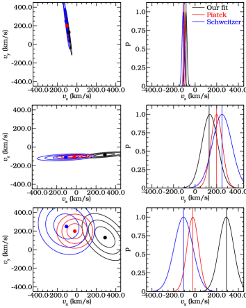
The joint and marginalised probability distribution functions for the velocity components of Sculptor are plotted in Fig. 12 together with the 1, 2 and 3 contours. The maximum likelihood value is reached at . These values are in agreement with Walker et al. (2008), who use a similar method. We also over plot the measurements of Piatek et al. (2006, in red) and Schweitzer et al. (1995, in blue) while the maximum likelihood value is indicated in black. Note that the uncertainty in is smallest since this reflects mainly the uncertainty in the mean radial velocity of the centre of mass of Sculptor due to its high galactic latitude. The uncertainties in the other two velocity components mainly reflect the uncertainties in the proper motion measurements. Our determination of the component agrees well with the various data sets, while the component appears to be systematically offset. Note however, that there is overlap at the 3 level, and the and contours for the joint and overlap as well. Perhaps this level of disagreement could be taken as an indication that there may be intrinsic rotation in the system. Nonetheless, we note that with this procedure we effectively have removed the observed gradient and no apparent rotation remains, whatever its origin.