Testing some f(R,T) gravity models from energy conditions

F. G. Alvarengaa111e-mail: f.g.alvarenga@gmail.com,   M. J. S. Houndjoa,b222e-mail: sthoundjo@yahoo.fr,  A. V. Monwanoub333e-mail: movins2008@yahoo.fr  and Jean B. Chabi Oroub444e-mail: jean.chabi@imsp-uac.org

aDepartamento de Ciências Naturais - CEUNES - Universidade Federal do Espírito Santo
CEP 29933-415 - São Mateus - ES, Brazil

bInstitut de Mathématiques et de Sciences Physiques (IMSP), 01 BP 613 Porto-Novo, Bénin

Abstract

We consider f(R,T)𝑓𝑅𝑇f(R,T) theory of gravity, where R𝑅R is the curvature scalar and T𝑇T the trace of the energy momentum tensor. Attention is attached to the special case, f(R,T)=R+2f(T)𝑓𝑅𝑇𝑅2𝑓𝑇f(R,T)=R+2f(T) and two expressions are assumed for the function f(T)𝑓𝑇f(T), a1Tn+b1a2Tn+b2subscript𝑎1superscript𝑇𝑛subscript𝑏1subscript𝑎2superscript𝑇𝑛subscript𝑏2\frac{a_{1}T^{n}+b_{1}}{a_{2}T^{n}+b_{2}} and a3lnq(b3Tm)subscript𝑎3superscript𝑞subscript𝑏3superscript𝑇𝑚a_{3}\ln^{q}{(b_{3}T^{m})}, where a1subscript𝑎1a_{1}, a2subscript𝑎2a_{2}, b1subscript𝑏1b_{1}, b2subscript𝑏2b_{2}, n𝑛n, a3subscript𝑎3a_{3}, b3subscript𝑏3b_{3}, q𝑞q and m𝑚m are input parameters. We observe that by adjusting suitably these input parameters, energy conditions can be satisfied. Moreover, an analyse of the perturbations and stabilities of de Sitter solutions and power-law solutions is performed with the use of the two models. The results show that for some values of the input parameters, for which energy conditions are satisfied, de Sitter solutions and power-law solutions may be stables.

Pacs numbers: 04.50.-h, 04.50.Kd, 98.80.-k

1 Introduction

It is well known that General Relativity (GR) based on the Einstein-Hilbert action (without taking into account the dark energy) can not explain the acceleration of the early and late universe. Therefore, GR does not describe precisely gravity and it is quite reasonable to modify it in order to get theories that admit inflation and imitate the dark energy. The first tentative in this way is substituting Einstein-Hilbert term by an arbitrary function of the curvature scalar R𝑅R, this is the so-called f(R)𝑅(R) theory of gravity. This theory has been widely studied and interesting results have been found [1]-[2]. In the same way, other alternative theory of modified gravity has been introduced, the so-called Gauss-Bonnet gravity, f(G)𝑓𝐺f(G), as a general function of the Gauss-Bonnet invariant term G𝐺G [3]. Other combinations of scalars are also used as the generalised f(R,G)𝑓𝑅𝐺f(R,G) and f(R,P,Q)𝑓𝑅𝑃𝑄f(R,P,Q) [4, 5], where PRμνRμν𝑃subscript𝑅𝜇𝜈superscript𝑅𝜇𝜈P\equiv R_{\mu\nu}R^{\mu\nu} and QRμνστRμνστ𝑄subscript𝑅𝜇𝜈𝜎𝜏superscript𝑅𝜇𝜈𝜎𝜏Q\equiv R_{\mu\nu\sigma\tau}R^{\mu\nu\sigma\tau} (here Rμνsubscript𝑅𝜇𝜈R_{\mu\nu} and Rμνστsubscript𝑅𝜇𝜈𝜎𝜏R_{\mu\nu\sigma\tau} are the Ricci tensor the Riemann tensor, respectively).

In this present paper, attention is attached to a type of the so-called f(R,T)𝑓𝑅𝑇f(R,T) theory of gravity, where T𝑇T denotes the trace of the energy momentum tensor. This generalization of f(R)𝑓𝑅f(R) gravity has been made first by Harko et al [6]. The dependence on T𝑇T can take source from the introduction of exotic imperfect fluid or from quantum effect (conformal anomaly). In this theory, the equations of motion show the presence of an extra-force acting on the test particles, and the motion are generally non-geodesic. This theory also relates the cosmic acceleration, not only due to the contribution of geometrical terms, but also to the matter contents [6]. Some results have been obtained with this theory. In [7], the cosmological reconstruction of f(R,T)𝑓𝑅𝑇f(R,T) describing transition from matter dominated phase to the late accelerated epoch of the universe is performed. Also in the same way for exploring cosmological scenarios based on this theory, f(R,T)𝑓𝑅𝑇f(R,T) function has been numerically reproduced according to holographic dark energy [8]. Moreover it is shown that dust reproduces ΛCDMΛ𝐶𝐷𝑀\Lambda CDM, phantom-non-phantom and the phantom cosmology with f(R,T)𝑓𝑅𝑇f(R,T) theory [9]. The general technique for performing this reproduction of ΛCDMΛ𝐶𝐷𝑀\Lambda CDM model in FRW555Friedmann-Robertson-Walker metric cosmological evolution is widely developed in [4, 10]. The f(R,T)𝑓𝑅𝑇f(R,T) models that are able to reproduce the fourth known types of future finite-time singularities have been investigated [11]. The authors also introduced conformal anomaly as quantum effects near the singularities and observe that it cannot remove the sudden singularity or the type IV one, but, for some values of a input parameter, the big rip and the type III singularity may be avoided from the effects of the conformal anomaly. Moreover, they found as interesting result that, even without taking into account conformal anomaly, singularities (the Big rip and the type-III) may still be removed thanks to the presence of the T𝑇T contribution of the f(R,T)𝑓𝑅𝑇f(R,T) theory.

Note that singularities appear when energy conditions are violated. Our task in this paper is to check the viability of some models of f(R,T)𝑓𝑅𝑇f(R,T) according to the energy conditions. The energy conditions are formulated by the use of the Raychaudhuri equation for expansion and is based on the attractive character of the gravity. We refer the readers to Refs [12]-[17], where energy conditions are widely analysed for the cosmology settings, in f(R) and f(G) gravities.

In this paper, we assume a special form of f(R,T)𝑓𝑅𝑇f(R,T), that is, f(R,T)=R+2f(T)𝑓𝑅𝑇𝑅2𝑓𝑇f(R,T)=R+2f(T), the usual Einstein-Hilbert term plus a T𝑇T dependent function f(T)𝑓𝑇f(T). Two expressions of f(T)𝑓𝑇f(T), a1Tn+b1a2Tn+b2subscript𝑎1superscript𝑇𝑛subscript𝑏1subscript𝑎2superscript𝑇𝑛subscript𝑏2\frac{a_{1}T^{n}+b_{1}}{a_{2}T^{n}+b_{2}} and a3lnq(b3Tm)subscript𝑎3superscript𝑞subscript𝑏3superscript𝑇𝑚a_{3}\ln^{q}{(b_{3}T^{m})} are investigated, where a1subscript𝑎1a_{1}, a2subscript𝑎2a_{2}, b1subscript𝑏1b_{1}, b2subscript𝑏2b_{2}, n𝑛n, a3subscript𝑎3a_{3}, b3subscript𝑏3b_{3}, q𝑞q and m𝑚m are parameters to be suitably adjusted in order to obtain viable models according to energy conditions. The first expression is similar to that used in [18, 19], where, at the place of the trace T𝑇T, the Gauss-Bonnet invariant is used. The main motivation of this choice is explained in the section 444. The second form is chosen due to its interesting aspect, because its corresponding f(R,T)𝑓𝑅𝑇f(R,T) model avoids itself the appearance of the type-I finite-time future singularity (Big Rip) [11], thanks to the ordinary trace T𝑇T-terms contributions. Thus it is quite reasonable to check for which values of the input parameters this model can be acceptable as cosmological model.

In order to reach the acceptable cosmological models, we analyse the perturbations and stabilities of de Sitter solutions and power-laws solutions in the framework of the special R+2f(T)𝑅2𝑓𝑇R+2f(T) gravity, by using the two models proposed in this work. We observe that for some values of the input parameters, for both models, the stabilities of de Sitter solutions and power-law solutions are realized and compatibles with some energy conditions and the late time acceleration of the universe.

The paper is outlined as follows. In section 222, we briefly present the general formalism of the theory, putting out the general equations of motion for a f(R,T)=f1(R)+f2(T)𝑓𝑅𝑇subscript𝑓1𝑅subscript𝑓2𝑇f(R,T)=f_{1}(R)+f_{2}(T) gravity, where f1(R)subscript𝑓1𝑅f_{1}(R) and f2(T)subscript𝑓2𝑇f_{2}(T) are respectively function of the curvature scalar and the trace of the energy momentum tensor. The section 333 is devoted to the general aspects of the energy conditions. The f(R,T)=R+2f(T)𝑓𝑅𝑇𝑅2𝑓𝑇f(R,T)=R+2f(T) gravity is assumed in the section 444, where the two functions considered for f(T)𝑓𝑇f(T) are studied, putting out the conditions on the input parameters for obtaining some viable models of f(R,T)𝑓𝑅𝑇f(R,T). The perturbations and stabilities of de Sitter and power-law solutions are investigated in the sections 555. Discussions and perspectives are presented in the section 666.

2 General formalism

Let us assume the modified gravity replacing the Ricci scalar R𝑅R in Einstein gravity by an arbitrary function f(R,T)𝑓𝑅𝑇f(R,T), and writing the total action as

S=12κ2d4xg[f(R,T)+],𝑆12superscript𝜅2superscript𝑑4𝑥𝑔delimited-[]𝑓𝑅𝑇\displaystyle S=\frac{1}{2\kappa^{2}}\int d^{4}x\sqrt{-g}\left[f(R,T)+\mathcal{L}\right]\,, (1)

where κ2=8πGsuperscript𝜅28𝜋𝐺\kappa^{2}=8\pi G, G𝐺G being the gravitational constant and T=gμνTμν𝑇superscript𝑔𝜇𝜈subscript𝑇𝜇𝜈T=g^{\mu\nu}T_{\mu\nu} the trace of the matter energy momentum tensor Tμνsubscript𝑇𝜇𝜈T_{\mu\nu} which is defined by

Tμν=2gδ(g)δgμν.subscript𝑇𝜇𝜈2𝑔𝛿𝑔𝛿superscript𝑔𝜇𝜈\displaystyle T_{\mu\nu}=-\frac{2}{\sqrt{-g}}\frac{\delta(\sqrt{-g}\mathcal{L})}{\delta g^{\mu\nu}}\,\,. (2)

This modified gravity theory has been considered first in [6] and the equations of motion, using the metric formalism, have been explicitly obtained as

fR(R,T)Rμν12f(R,T)gμν+(gμνμν)fR(R,T)=κ2TμνfT(R,T)TμνfT(R,T)Θμν,subscript𝑓𝑅𝑅𝑇subscript𝑅𝜇𝜈12𝑓𝑅𝑇subscript𝑔𝜇𝜈subscript𝑔𝜇𝜈subscript𝜇subscript𝜈subscript𝑓𝑅𝑅𝑇superscript𝜅2subscript𝑇𝜇𝜈subscript𝑓𝑇𝑅𝑇subscript𝑇𝜇𝜈subscript𝑓𝑇𝑅𝑇subscriptΘ𝜇𝜈\displaystyle f_{R}(R,T)R_{\mu\nu}-\frac{1}{2}f(R,T)g_{\mu\nu}+\left(g_{\mu\nu}\Box-\nabla_{\mu}\nabla_{\nu}\right)f_{R}(R,T)=\kappa^{2}T_{\mu\nu}-f_{T}(R,T)T_{\mu\nu}-f_{T}(R,T)\Theta_{\mu\nu}\,, (3)

where fR(R,T)subscript𝑓𝑅𝑅𝑇f_{R}(R,T) and fT(R,T)subscript𝑓𝑇𝑅𝑇f_{T}(R,T) denote the derivative of f(R, T) with respect to R and T, respectively, and ΘμνsubscriptΘ𝜇𝜈\Theta_{\mu\nu} is defined by [6]

ΘμνgαβδTαβδgμν=2Tμν+gμν2gαβ2gμνgαβ.subscriptΘ𝜇𝜈superscript𝑔𝛼𝛽𝛿subscript𝑇𝛼𝛽𝛿superscript𝑔𝜇𝜈2subscript𝑇𝜇𝜈subscript𝑔𝜇𝜈2superscript𝑔𝛼𝛽superscript2superscript𝑔𝜇𝜈superscript𝑔𝛼𝛽\displaystyle\Theta_{\mu\nu}\equiv g^{\alpha\beta}\frac{\delta T_{\alpha\beta}}{\delta g^{\mu\nu}}=-2T_{\mu\nu}+g_{\mu\nu}\mathcal{L}-2g^{\alpha\beta}\frac{\partial^{2}\mathcal{L}}{\partial g^{\mu\nu}\partial g^{\alpha\beta}}\,\,. (4)

Let us consider the stress-energy tensor of the matter as

Tμν=(ρ+p)uμuνpgμν.subscript𝑇𝜇𝜈𝜌𝑝subscript𝑢𝜇subscript𝑢𝜈𝑝subscript𝑔𝜇𝜈\displaystyle T_{\mu\nu}=(\rho+p)u_{\mu}u_{\nu}-pg_{\mu\nu}\,\,. (5)

This expression is a consequence of a statement of the fluid mechanics for which a possible way for treating the scalar invariant \mathcal{L} is to interpret it as the pressure p of the fluid, i.e. =p𝑝\mathcal{L}=-p (the negative sign is due to the signature used here) [6, 16]. Here, ρ𝜌\rho, p𝑝p and uμsuperscript𝑢𝜇u^{\mu} are respectively the energy density, the pressure and the four-velocity of a perfect fluid considered as the classical matter content of the universe. Hence, Eq.(4) becomes

Θμν=2Tμνpgμν.subscriptΘ𝜇𝜈2subscript𝑇𝜇𝜈𝑝subscript𝑔𝜇𝜈\displaystyle\Theta_{\mu\nu}=-2T_{\mu\nu}-pg_{\mu\nu}\,\,. (6)

From now, we will treat the models of type f(R,T)=f1(R)+f2(T)𝑓𝑅𝑇subscript𝑓1𝑅subscript𝑓2𝑇f(R,T)=f_{1}(R)+f_{2}(T) and set κ2=1superscript𝜅21\kappa^{2}=1. Then, the equation (3) becomes

f1R(R)Rμν12f1(R)gμν+(gμνμν)f1R(R)=Tμν+f2T(T)Tμν+[f2T(T)p+12f2(T)]gμνsubscript𝑓1𝑅𝑅subscript𝑅𝜇𝜈12subscript𝑓1𝑅subscript𝑔𝜇𝜈subscript𝑔𝜇𝜈subscript𝜇subscript𝜈subscript𝑓1𝑅𝑅subscript𝑇𝜇𝜈subscript𝑓2𝑇𝑇subscript𝑇𝜇𝜈delimited-[]subscript𝑓2𝑇𝑇𝑝12subscript𝑓2𝑇subscript𝑔𝜇𝜈\displaystyle f_{1R}(R)R_{\mu\nu}-\frac{1}{2}f_{1}(R)g_{\mu\nu}+\left(g_{\mu\nu}\Box-\nabla_{\mu}\nabla_{\nu}\right)f_{1R}(R)=T_{\mu\nu}+f_{2T}(T)T_{\mu\nu}+\left[f_{2T}(T)p+\frac{1}{2}f_{2}(T)\right]g_{\mu\nu} (7)

3 Energy conditions

The energy conditions are essentially based on the Raychaudhuri equation that describes the behaviour of a congruence of timelike, spacelike or lightlike curves. It is commonly used to study and establish singularities of the spacetime. Considering a congruence of the curves fulfilling the spacetime manifold and also that there are expansion, distortion and relative rotation between the curves of the congruence, then the spacetime manifold described by the congruence is curved. For the purposes of this work we will just consider the timelike and spacelike curves for which the Raychaudhuri equation reads, respectively [20, 21]

RμνVμVν+13θ2+σμνσμνωμνωμν+dθdτ=0,subscript𝑅𝜇𝜈superscript𝑉𝜇superscript𝑉𝜈13superscript𝜃2subscript𝜎𝜇𝜈superscript𝜎𝜇𝜈subscript𝜔𝜇𝜈superscript𝜔𝜇𝜈𝑑𝜃𝑑𝜏0\displaystyle R_{\mu\nu}V^{\mu}V^{\nu}+\frac{1}{3}\theta^{2}+\sigma_{\mu\nu}\sigma^{\mu\nu}-\omega_{\mu\nu}\omega^{\mu\nu}+\frac{d\theta}{d\tau}=0\,\,, (8)
Rμνkμkν+12θ2+σμνσμνωμνωμν+dθdλ=0,subscript𝑅𝜇𝜈superscript𝑘𝜇superscript𝑘𝜈12superscript𝜃2subscript𝜎𝜇𝜈superscript𝜎𝜇𝜈subscript𝜔𝜇𝜈superscript𝜔𝜇𝜈𝑑𝜃𝑑𝜆0\displaystyle R_{\mu\nu}k^{\mu}k^{\nu}+\frac{1}{2}\theta^{2}+\sigma_{\mu\nu}\sigma^{\mu\nu}-\omega_{\mu\nu}\omega^{\mu\nu}+\frac{d\theta}{d\lambda}=0\,\,, (9)

where θ𝜃\theta is the expansion scalar describing the expansion of volume, τ𝜏\tau and λ𝜆\lambda are positive parameters used to describe the curved of the congruence, σμνsubscript𝜎𝜇𝜈\sigma_{\mu\nu} the shear tensor which measures the distortion of the volume, ωμνsubscript𝜔𝜇𝜈\omega_{\mu\nu} the vorticity tensor which measures the rotation of the curves, and Vμsuperscript𝑉𝜇V^{\mu} and kμsuperscript𝑘𝜇k^{\mu} are respectively timelike and lightlike vectors tangent to the curves. In this work, we are interested to the situation for small distortions of the volume, without rotation, in such a way that the quadratic terms in the Raychaudhuri equation may be disregarded (they are like second order corrections). Then, the equation can be integrated given the scalar of expansion as a function of the Ricci tensor:

θ=τRμνVμVν=λRμνkμkν.𝜃𝜏subscript𝑅𝜇𝜈superscript𝑉𝜇superscript𝑉𝜈𝜆subscript𝑅𝜇𝜈superscript𝑘𝜇superscript𝑘𝜈\displaystyle\theta=-\tau R_{\mu\nu}V^{\mu}V^{\nu}=-\lambda R_{\mu\nu}k^{\mu}k^{\nu}\,\,. (10)

The condition for attractive gravity is θ<0𝜃0\theta<0, imposing RμνVμVν0subscript𝑅𝜇𝜈superscript𝑉𝜇superscript𝑉𝜈0R_{\mu\nu}V^{\mu}V^{\nu}\geq 0 and Rμνkμkν0subscript𝑅𝜇𝜈superscript𝑘𝜇superscript𝑘𝜈0R_{\mu\nu}k^{\mu}k^{\nu}\geq 0. These two conditions are called the strong and null energy conditions, respectively.

For equivalence to GR, by just dividing by f1(R)subscript𝑓1𝑅f_{1}(R) (different from zero), one can cast Eq. (7) in the following form

Rμν12Rgμν=Tμνeff,subscript𝑅𝜇𝜈12𝑅subscript𝑔𝜇𝜈superscriptsubscript𝑇𝜇𝜈𝑒𝑓𝑓\displaystyle R_{\mu\nu}-\frac{1}{2}Rg_{\mu\nu}=T_{\mu\nu}^{eff}\,\,\,, (11)

where the effective energy momentum tensor Tμνeffsuperscriptsubscript𝑇𝜇𝜈𝑒𝑓𝑓T_{\mu\nu}^{eff} is defined by

Tμνeff=1f1R(R){Tμν+f2T(T)Tμν+12[2f2T(T)p+f2(T)+f1(R)Rf1R(R)]gμν\displaystyle T_{\mu\nu}^{eff}=\frac{1}{f_{1R}(R)}\Big{\{}T_{\mu\nu}+f_{2T}(T)T_{\mu\nu}+\frac{1}{2}\left[2f_{2T}(T)p+f_{2}(T)+f_{1}(R)-Rf_{1R}(R)\right]g_{\mu\nu}
(gμνμν)f1R(R)}.\displaystyle-\left(g_{\mu\nu}\Box-\nabla_{\mu}\nabla_{\nu}\right)f_{1R}(R)\Big{\}}\,\,\,. (12)

Since the vector field kμsuperscript𝑘𝜇k^{\mu} is lightlike, one gets kμkμ=0superscript𝑘𝜇subscript𝑘𝜇0k^{\mu}k_{\mu}=0. Then, by multiplying Eq. (11) by the bi-vector kμkνsuperscript𝑘𝜇superscript𝑘𝜈k^{\mu}k^{\nu}, the null energy condition comes to be equivalent to Tμνeffkμkν0superscriptsubscript𝑇𝜇𝜈𝑒𝑓𝑓superscript𝑘𝜇superscript𝑘𝜈0T_{\mu\nu}^{eff}k^{\mu}k^{\nu}\geq 0. Remark also that Eq. (11) is equivalent to

Rμν=Tμνeff12Teffgμν.subscript𝑅𝜇𝜈subscriptsuperscript𝑇𝑒𝑓𝑓𝜇𝜈12superscript𝑇𝑒𝑓𝑓subscript𝑔𝜇𝜈\displaystyle R_{\mu\nu}=T^{eff}_{\mu\nu}-\frac{1}{2}T^{eff}g_{\mu\nu}\,\,\,. (13)

Then, the strong energy condition reads (Tμνeff12Teffgμν)VμVν0subscriptsuperscript𝑇𝑒𝑓𝑓𝜇𝜈12superscript𝑇𝑒𝑓𝑓subscript𝑔𝜇𝜈superscript𝑉𝜇superscript𝑉𝜈0\left(T^{eff}_{\mu\nu}-\frac{1}{2}T^{eff}g_{\mu\nu}\right)V^{\mu}V^{\nu}\geq 0. By assuming that the total content of the universe behaves as perfect fluid, Eq. (5) also holds, by just substituting ρ𝜌\rho and p𝑝p, by ρeffsubscript𝜌𝑒𝑓𝑓\rho_{eff} and peffsubscript𝑝𝑒𝑓𝑓p_{eff} respectively (the effective energy density and effective pressure). Thus, the null energy condition imposes

Teffμνkμkν=(ρeff+peff)uμuνkμkνpeffgμνkμkν0.superscriptsubscript𝑇𝑒𝑓𝑓𝜇𝜈superscript𝑘𝜇superscript𝑘𝜈subscript𝜌𝑒𝑓𝑓subscript𝑝𝑒𝑓𝑓subscript𝑢𝜇subscript𝑢𝜈superscript𝑘𝜇superscript𝑘𝜈subscript𝑝𝑒𝑓𝑓subscript𝑔𝜇𝜈superscript𝑘𝜇superscript𝑘𝜈0\displaystyle T_{eff}^{\mu\nu}k^{\mu}k^{\nu}=\left(\rho_{eff}+p_{eff}\right)u_{\mu}u_{\nu}k^{\mu}k^{\nu}-p_{eff}g_{\mu\nu}k^{\mu}k^{\nu}\geq 0\,\,\,. (14)

Since, kμsuperscript𝑘𝜇k^{\mu} is a lightlike vector, one has gμνkμkν=kμkμ=0subscript𝑔𝜇𝜈superscript𝑘𝜇superscript𝑘𝜈superscript𝑘𝜇subscript𝑘𝜇0g_{\mu\nu}k^{\mu}k^{\nu}=k^{\mu}k_{\mu}=0. Also, we always get uμuνkμkν=(uμkμ)2>0subscript𝑢𝜇subscript𝑢𝜈superscript𝑘𝜇superscript𝑘𝜈superscriptsubscript𝑢𝜇superscript𝑘𝜇20u_{\mu}u_{\nu}k^{\mu}k^{\nu}=(u_{\mu}k^{\mu})^{2}>0. Thus, the null energy condition for the effective perfect fluid reduces to

ρeff+peff0.subscript𝜌𝑒𝑓𝑓subscript𝑝𝑒𝑓𝑓0\displaystyle\rho_{eff}+p_{eff}\geq 0\,\,\,. (15)

For the strong energy condition, one has

(Tμν12Tgμν)VμVνsubscript𝑇𝜇𝜈12𝑇subscript𝑔𝜇𝜈superscript𝑉𝜇superscript𝑉𝜈\displaystyle\left(T_{\mu\nu}-\frac{1}{2}Tg_{\mu\nu}\right)V^{\mu}V^{\nu} =\displaystyle= [(ρeff+peff)uμuνpeffgμν12(ρeff3peff)gμν]VμVμ0,delimited-[]subscript𝜌𝑒𝑓𝑓subscript𝑝𝑒𝑓𝑓subscript𝑢𝜇subscript𝑢𝜈subscript𝑝𝑒𝑓𝑓subscript𝑔𝜇𝜈12subscript𝜌𝑒𝑓𝑓3subscript𝑝𝑒𝑓𝑓subscript𝑔𝜇𝜈superscript𝑉𝜇superscript𝑉𝜇0\displaystyle\left[\left(\rho_{eff}+p_{eff}\right)u_{\mu}u_{\nu}-p_{eff}g_{\mu\nu}-\frac{1}{2}\left(\rho_{eff}-3p_{eff}\right)g_{\mu\nu}\right]V^{\mu}V^{\mu}\geq 0\,\,\,, (16)
=\displaystyle= (ρeff+3peff)VμVμsubscript𝜌𝑒𝑓𝑓3subscript𝑝𝑒𝑓𝑓superscript𝑉𝜇subscript𝑉𝜇\displaystyle\left(\rho_{eff}+3p_{eff}\right)V^{\mu}V_{\mu} (17)

where we made use of Teff=ρeff3peffsuperscript𝑇𝑒𝑓𝑓subscript𝜌𝑒𝑓𝑓3subscript𝑝𝑒𝑓𝑓T^{eff}=\rho_{eff}-3p_{eff} and uμuνVμVν=VμVμsubscript𝑢𝜇subscript𝑢𝜈superscript𝑉𝜇superscript𝑉𝜈subscript𝑉𝜇superscript𝑉𝜇u_{\mu}u_{\nu}V^{\mu}V^{\nu}=V_{\mu}V^{\mu} for obtaining the second equality.666 Since uμsubscript𝑢𝜇u_{\mu} is an unitary timelike vector (four-velocity) and the metric component g00=g00=1subscript𝑔00superscript𝑔001g_{00}=g^{00}=1 (see Eq. (24)), one gets uμuνVμVν=VμVμsubscript𝑢𝜇subscript𝑢𝜈superscript𝑉𝜇superscript𝑉𝜈subscript𝑉𝜇superscript𝑉𝜇u_{\mu}u_{\nu}V^{\mu}V^{\nu}=V_{\mu}V^{\mu}. Remark that the condition (16) is equivalent to

(ρeff+peff)VμVμ12(ρeffpeff)VμVμ,subscript𝜌𝑒𝑓𝑓subscript𝑝𝑒𝑓𝑓superscript𝑉𝜇subscript𝑉𝜇12subscript𝜌𝑒𝑓𝑓subscript𝑝𝑒𝑓𝑓superscript𝑉𝜇subscript𝑉𝜇\displaystyle\left(\rho_{eff}+p_{eff}\right)V^{\mu}V_{\mu}\geq\frac{1}{2}\left(\rho_{eff}-p_{eff}\right)V^{\mu}V_{\mu}\,\,\,, (18)

which imposes (ρeff+peff)VμVμ0subscript𝜌𝑒𝑓𝑓subscript𝑝𝑒𝑓𝑓superscript𝑉𝜇subscript𝑉𝜇0\left(\rho_{eff}+p_{eff}\right)V^{\mu}V_{\mu}\geq 0. Since the vector Vμsuperscript𝑉𝜇V^{\mu} is timelike, one has VμVμ0superscript𝑉𝜇subscript𝑉𝜇0V^{\mu}V_{\mu}\geq 0, and the strong energy condition reduces to

ρeff+peff0,ρeff+3peff0.formulae-sequencesubscript𝜌𝑒𝑓𝑓subscript𝑝𝑒𝑓𝑓0subscript𝜌𝑒𝑓𝑓3subscript𝑝𝑒𝑓𝑓0\displaystyle\rho_{eff}+p_{eff}\geq 0\,\,\,,\quad\quad\rho_{eff}+3p_{eff}\geq 0\,\,\,\,. (19)

Note that the condition (Tμνeff12Teffgμν)VμVν0subscriptsuperscript𝑇𝑒𝑓𝑓𝜇𝜈12superscript𝑇𝑒𝑓𝑓subscript𝑔𝜇𝜈superscript𝑉𝜇superscript𝑉𝜈0\left(T^{eff}_{\mu\nu}-\frac{1}{2}T^{eff}g_{\mu\nu}\right)V^{\mu}V^{\nu}\geq 0 is equivalent to TμνeffVμVν12TeffVμVνsubscriptsuperscript𝑇𝑒𝑓𝑓𝜇𝜈superscript𝑉𝜇superscript𝑉𝜈12superscript𝑇𝑒𝑓𝑓superscript𝑉𝜇subscript𝑉𝜈T^{eff}_{\mu\nu}V^{\mu}V^{\nu}\geq\frac{1}{2}T^{eff}V^{\mu}V_{\nu}. This requires to have the necessary condition TμνeffVμVν0subscriptsuperscript𝑇𝑒𝑓𝑓𝜇𝜈superscript𝑉𝜇superscript𝑉𝜈0T^{eff}_{\mu\nu}V^{\mu}V^{\nu}\geq 0. The weak energy condition requires to this condition holds for any non-spacelike vector [20, 22]. This means that the condition holds for both lightlike and timelike vectors. The use of the lightlike vector is equivalent to the null energy condition as previously demonstrated. Now, for a timelike vector, one gets

TμνeffVμVνsubscriptsuperscript𝑇𝑒𝑓𝑓𝜇𝜈superscript𝑉𝜇superscript𝑉𝜈\displaystyle T^{eff}_{\mu\nu}V^{\mu}V^{\nu} =\displaystyle= [(ρeff+peff)uμuνpeffgμν]VμVν0,delimited-[]subscript𝜌𝑒𝑓𝑓subscript𝑝𝑒𝑓𝑓subscript𝑢𝜇subscript𝑢𝜈subscript𝑝𝑒𝑓𝑓subscript𝑔𝜇𝜈superscript𝑉𝜇superscript𝑉𝜈0\displaystyle\left[\left(\rho_{eff}+p_{eff}\right)u_{\mu}u_{\nu}-p_{eff}g_{\mu\nu}\right]V^{\mu}V^{\nu}\geq 0\,\,\,, (20)
=\displaystyle= ρeffVμVμ0.subscript𝜌𝑒𝑓𝑓superscript𝑉𝜇subscript𝑉𝜇0\displaystyle\rho_{eff}V^{\mu}V_{\mu}\geq 0\,\,\,.

Since, Vμsuperscript𝑉𝜇V^{\mu} is a timelike vector, one always has VμVμ0superscript𝑉𝜇subscript𝑉𝜇0V^{\mu}V_{\mu}\geq 0. Thus, the weak energy condition for the effective perfect fluid reads

ρeff0,(ρeff+peff)0.formulae-sequencesubscript𝜌𝑒𝑓𝑓0subscript𝜌𝑒𝑓𝑓subscript𝑝𝑒𝑓𝑓0\displaystyle\rho_{eff}\geq 0\,\,\,,\quad\quad\quad\left(\rho_{eff}+p_{eff}\right)\geq 0\,\,\,. (21)

For the dominant energy condition, the required condition is that, besides the weak energy condition, for any timelike vector Vμsuperscript𝑉𝜇V^{\mu}, TμνVμsubscript𝑇𝜇𝜈superscript𝑉𝜇T_{\mu\nu}V^{\mu} is a non-spacelike vector. In other word, this means that no signal can propagate faster than light. It follows that peffρeffsubscript𝑝𝑒𝑓𝑓subscript𝜌𝑒𝑓𝑓p_{eff}\leq\rho_{eff}, since, for any know matter, pressures are small when the energy density is small. Thus, the dominant energy condition results in

ρeff0,ρeff+peff0,ρeffpeff0.formulae-sequencesubscript𝜌𝑒𝑓𝑓0formulae-sequencesubscript𝜌𝑒𝑓𝑓subscript𝑝𝑒𝑓𝑓0subscript𝜌𝑒𝑓𝑓subscript𝑝𝑒𝑓𝑓0\displaystyle\rho_{eff}\geq 0\,\,,\quad\quad\rho_{eff}+p_{eff}\geq 0\,\,,\quad\quad\quad\rho_{eff}-p_{eff}\geq 0\,\,\,. (22)

Therefore, the energy conditions, as known in GR, can also be applied in this modified theory of gravity by substituting the ordinary energy density ρ𝜌\rho and pressure p𝑝p in GR by the effective ones, ρeffsubscript𝜌𝑒𝑓𝑓\rho_{eff} and peffsubscript𝑝𝑒𝑓𝑓p_{eff}.

In what follows, we will consider models of type f(R,T)=R+2f(T)𝑓𝑅𝑇𝑅2𝑓𝑇f(R,T)=R+2f(T), i.e., the usual Einstein-Hilbert term plus trace depending term 2f(T)2𝑓𝑇2f(T). This amounts to consider f1(R)=Rsubscript𝑓1𝑅𝑅f_{1}(R)=R and f2(T)=2f(T)subscript𝑓2𝑇2𝑓𝑇f_{2}(T)=2f(T). The factor 222 is used just for letting the field equations more easier to be treated. We will also assume that the ordinary content of the universe is pressureless and satisfies the energy conditions (just ρ0𝜌0\rho\geq 0).

4 Testing some f(R,T)=R+2f(T)𝑓𝑅𝑇𝑅2𝑓𝑇f(R,T)=R+2f(T) models from energy conditions

In this section we will present the conditions required on ρ𝜌\rho and the algebraic function f(T)𝑓𝑇f(T) for realizing each type of energy conditions. For this end, we first need to establish the respective expression of the effective energy density ρeffsubscript𝜌𝑒𝑓𝑓\rho_{eff} and effective pressure peffsubscript𝑝𝑒𝑓𝑓p_{eff}. According to the assumptions made at the end of the previous section, Eq. (7) becomes

Rμν12Rgμν=Tμν+2fT(T)Tμν+f(T)gμν.subscript𝑅𝜇𝜈12𝑅subscript𝑔𝜇𝜈subscript𝑇𝜇𝜈2subscript𝑓𝑇𝑇subscript𝑇𝜇𝜈𝑓𝑇subscript𝑔𝜇𝜈\displaystyle R_{\mu\nu}-\frac{1}{2}Rg_{\mu\nu}=T_{\mu\nu}+2f_{T}(T)T_{\mu\nu}+f(T)g_{\mu\nu}\,\,. (23)

Considering the flat FRW space-time described by the metric

ds2=dt2a2(t)d𝐱2,𝑑superscript𝑠2𝑑superscript𝑡2superscript𝑎2𝑡𝑑superscript𝐱2\displaystyle ds^{2}=dt^{2}-a^{2}(t)d{\bf x}^{2}\,\,, (24)

where a(t)𝑎𝑡a(t) is the scale factor. The 000000 and ii𝑖𝑖ii components of (23) can be written as

3H23superscript𝐻2\displaystyle 3H^{2} =\displaystyle= ρeff,subscript𝜌𝑒𝑓𝑓\displaystyle\rho_{eff}\,\,, (25)
2H˙3H22˙𝐻3superscript𝐻2\displaystyle-2\dot{H}-3H^{2} =\displaystyle= peff,subscript𝑝𝑒𝑓𝑓\displaystyle p_{eff}\,\,, (26)

where the effective energy density and pressure are defined as

ρeffsubscript𝜌𝑒𝑓𝑓\displaystyle\rho_{eff} =\displaystyle= ρ+2ρfT(T)+f(T),𝜌2𝜌subscript𝑓𝑇𝑇𝑓𝑇\displaystyle\rho+2\rho f_{T}(T)+f(T)\,\,, (27)
peffsubscript𝑝𝑒𝑓𝑓\displaystyle p_{eff} =\displaystyle= f(T).𝑓𝑇\displaystyle-f(T)\,\,. (28)

By using the above expressions of the effective energy density and pressure, we get the null energy condition (NEC), the weak energy condition (WEC), the strong energy condition (SEC) and the dominant energy condition (DEC) by

NEC:ρeff+peff=ρ[1+2fT(T)]0,NEC:subscript𝜌𝑒𝑓𝑓subscript𝑝𝑒𝑓𝑓𝜌delimited-[]12subscript𝑓𝑇𝑇0\displaystyle\mbox{NEC:}\quad\quad\quad\quad\quad\quad\rho_{eff}+p_{eff}=\rho\left[1+2f_{T}(T)\right]\geq 0\,\,\,, (29)
WEC:ρeff=ρ+2ρfT(T)+f(T)0,ρeff+peff0,formulae-sequenceWEC:subscript𝜌𝑒𝑓𝑓𝜌2𝜌subscript𝑓𝑇𝑇𝑓𝑇0subscript𝜌𝑒𝑓𝑓subscript𝑝𝑒𝑓𝑓0\displaystyle\mbox{WEC:}\quad\quad\quad\quad\quad\quad\rho_{eff}=\rho+2\rho f_{T}(T)+f(T)\geq 0\,\,,\quad\rho_{eff}+p_{eff}\geq 0\,\,\,, (30)
SEC:ρeff+3peff=ρ+2ρfT(T)2f(T)0,ρeff+peff0,formulae-sequenceSEC:subscript𝜌𝑒𝑓𝑓3subscript𝑝𝑒𝑓𝑓𝜌2𝜌subscript𝑓𝑇𝑇2𝑓𝑇0subscript𝜌𝑒𝑓𝑓subscript𝑝𝑒𝑓𝑓0\displaystyle\mbox{SEC:}\quad\quad\quad\quad\rho_{eff}+3p_{eff}=\rho+2\rho f_{T}(T)-2f(T)\geq 0\,\,,\quad\rho_{eff}+p_{eff}\geq 0\,\,, (31)
DEC:ρeffpeff=ρ+2ρfT(T)+2f(T)0,ρeff+peff0,ρeff0.formulae-sequenceDEC:subscript𝜌𝑒𝑓𝑓subscript𝑝𝑒𝑓𝑓𝜌2𝜌subscript𝑓𝑇𝑇2𝑓𝑇0formulae-sequencesubscript𝜌𝑒𝑓𝑓subscript𝑝𝑒𝑓𝑓0subscript𝜌𝑒𝑓𝑓0\displaystyle\mbox{DEC:}\quad\quad\quad\rho_{eff}-p_{eff}=\rho+2\rho f_{T}(T)+2f(T)\geq 0\,\,,\quad\rho_{eff}+p_{eff}\geq 0\,\,,\quad\rho_{eff}\geq 0\,\,. (32)

We propose to test two models of f(T)𝑓𝑇f(T) in the way to make them satisfying the energy conditions. For the first model, we consider a function f(T)𝑓𝑇f(T) such that for large and small values of the trace, it converges. We start by assuming first this function as f(T)=a1Tn+b1a2Tn+b2𝑓𝑇subscript𝑎1superscript𝑇𝑛subscript𝑏1subscript𝑎2superscript𝑇𝑛subscript𝑏2f(T)=\frac{a_{1}T^{n}+b_{1}}{a_{2}T^{n}+b_{2}}, where a1subscript𝑎1a_{1}, a2subscript𝑎2a_{2}, b1subscript𝑏1b_{1}, b2subscript𝑏2b_{2} and n𝑛n are parameters to be adjusted in order to obtain models that satisfy some or all the energy conditions. Note that this expression is similar to that used in [18, 19], where, at the place of the trace T𝑇T, the Gauss-Bonnet invariant is used. A motivation in using this model is that when n>0𝑛0n>0, it prevents divergence for large and small values of the trace777This requires to fix a20subscript𝑎20a_{2}\neq 0 for large values of trace and b20subscript𝑏20b_{2}\neq 0 for small values of the trace.. Remark that for T𝑇T\rightarrow\infty, f(T)=a1/a2𝑓𝑇subscript𝑎1subscript𝑎2f(T)=a_{1}/a_{2} is finite, and for T0𝑇0T\rightarrow 0, f(T)=b1/b2𝑓𝑇subscript𝑏1subscript𝑏2f(T)=b_{1}/b_{2} which is also finite. However, when n<0𝑛0n<0, the situation inverts, and for large and small values of the trace888This requires to fix a20subscript𝑎20a_{2}\neq 0 for small values of trace and b20subscript𝑏20b_{2}\neq 0 for large values of the trace., one obtains f(T)=b1/b2𝑓𝑇𝑏1𝑏2f(T)=b1/b2 and f(T)=a1/a2𝑓𝑇𝑎1𝑎2f(T)=a1/a2, respectively, and the divergence is still prevented. But note that all this is a mathematical point of view, which also may be useful at the physical point of view. Let us now explore the cosmological feature of this model. Here we can discuss the occurrence of cosmic acceleration, which may impose some constraints to the parameters, reducing the degree of freedom of the model. Searching for the power-like solutions, one has: a=a0tx𝑎subscript𝑎0superscript𝑡𝑥a=a_{0}t^{x}, H=xt1𝐻𝑥superscript𝑡1H=xt^{-1}, H˙=xt2˙𝐻𝑥superscript𝑡2\dot{H}=-xt^{-2} and f(T)g(t)=(a¯1t3xn+b1)/(a¯2t3xn+b2)𝑓𝑇𝑔𝑡subscript¯𝑎1superscript𝑡3𝑥𝑛subscript𝑏1subscript¯𝑎2superscript𝑡3𝑥𝑛subscript𝑏2f(T)\rightarrow g(t)=(\bar{a}_{1}t^{-3xn}+b_{1})/(\bar{a}_{2}t^{-3xn}+b_{2}), with a¯i=aiρ0a03subscript¯𝑎𝑖subscript𝑎𝑖subscript𝜌0superscriptsubscript𝑎03\bar{a}_{i}=a_{i}\rho_{0}a_{0}^{-3} (i=1,2𝑖12i=1,2), where we used T=ρ=ρa3𝑇𝜌𝜌superscript𝑎3T=\rho=\rho a^{-3} (because the ordinary content of the universe is dust). With the scale factor being used here, the early universe corresponds to t0𝑡0t\rightarrow 0 and the late time correspond to t𝑡t\rightarrow\infty, where x>0𝑥0x>0. At early time, the curvature scalar R𝑅R\rightarrow\infty (where the f(T)𝑓𝑇f(T) contribution may be neglected) and at late-time, the universe may be characterized by the ΛCDMΛ𝐶𝐷𝑀\Lambda CDM model, i.e., our model must behave like R+2Λ𝑅2ΛR+2\Lambda. For obtaining this feature, for n<0𝑛0n<0, the cosmological constant reads Λ=a¯1/a¯2=a1/a2Λsubscript¯𝑎1subscript¯𝑎2subscript𝑎1subscript𝑎2\Lambda=\bar{a}_{1}/\bar{a}_{2}=a_{1}/a_{2}, while for n>0𝑛0n>0, one gets Λ=b1/b2Λsubscript𝑏1subscript𝑏2\Lambda={b}_{1}/{b}_{2}. By calling ωeffsubscript𝜔𝑒𝑓𝑓\omega_{eff} the effective parameter of the equation of state, one has ωeff=peff/ρeff=f(T)/(ρ+2ρfρ+f(T))subscript𝜔𝑒𝑓𝑓subscript𝑝𝑒𝑓𝑓subscript𝜌𝑒𝑓𝑓𝑓𝑇𝜌2𝜌subscript𝑓𝜌𝑓𝑇\omega_{eff}={p_{eff}}/\rho_{eff}=-f(T)/(\rho+2\rho f_{\rho}+f(T)). The requirement of guaranteeing the acceleration of the universe, without falling into phantom model, is 1<ωeff<1/31subscript𝜔𝑒𝑓𝑓13-1<\omega_{eff}<-1/3. Observe that at time, (t𝑡t\rightarrow\infty), ωeff=1subscript𝜔𝑒𝑓𝑓1\omega_{eff}=-1 (this holds only when n>0𝑛0n>0). Thus, we see that some values of the input parameters can make the model providing the late time acceleration, i.e., for n>0𝑛0n>0, a1/a2>0subscript𝑎1subscript𝑎20a_{1}/a_{2}>0 and b1/b2=Λsubscript𝑏1subscript𝑏2Λb_{1}/b_{2}=\Lambda. It is important to note that when the acceleration is guaranteed, at least the strong energy condition is violated. But here, we recall that the aim of this work is to find the range of the parameters for which the energy conditions are satisfied. We will develop this in the subsection 4.14.1{\bf 4.1}.

For the second model, we assume f(T)=a3lnq(b3Tm)𝑓𝑇subscript𝑎3superscript𝑞subscript𝑏3superscript𝑇𝑚f(T)=a_{3}\ln^{q}{\left(b_{3}T^{m}\right)} where a3subscript𝑎3a_{3}, m𝑚m and q𝑞q are also adjustable parameters and b3subscript𝑏3b_{3} is assumed to be positive and non null. This form is chosen due to its interesting aspect, because it is a type of the f(T)𝑓𝑇f(T) model for which, the future finite-time singularity of type-I (the Big Rip) can be cured in f(R,T)=R+2f(T)𝑓𝑅𝑇𝑅2𝑓𝑇f(R,T)=R+2f(T) gravity [11]. Despite the aim of this work not being the study of the avoidance of singularities, we can try to show a little more how this type of model can prevent the Big Rip. Remember that the Big Rip is the type of the future finite-time singularity for which, the scale factor, the energy density and the pressure diverge. This also implies that at the singularity time, here denoted by tssubscript𝑡𝑠t_{s}, the curvature scalar R𝑅R diverges. Then, in order to show the avoidance of the Big Rip from the contribution of the f(T)𝑓𝑇f(T), let us take the trace of the Eq. (23), i.e.

R=ρ+2ρfT(T)+4f(T).𝑅𝜌2𝜌subscript𝑓𝑇𝑇4𝑓𝑇\displaystyle-R=\rho+2\rho f_{T}(T)+4f(T)\,\,\,. (33)

Remark that in [11], the Hubble parameter is written as H=h(tst)α𝐻superscriptsubscript𝑡𝑠𝑡𝛼H=h(t_{s}-t)^{-\alpha}, where hh is a positive real parameter and α>1𝛼1\alpha>1; this is the condition for the appearance of the Big Rip. In this case, the scale factor reads a=a¯exp[h(tst)1α/(α1)]𝑎¯𝑎𝑒𝑥𝑝delimited-[]superscriptsubscript𝑡𝑠𝑡1𝛼𝛼1a=\bar{a}exp{\left[h(t_{s}-t)^{1-\alpha}/(\alpha-1)\right]}, where a¯¯𝑎\bar{a} is a positive parameter. Hence, as the singularity is approached, the curvature R𝑅R behaves like (tst)2αsuperscriptsubscript𝑡𝑠𝑡2𝛼(t_{s}-t)^{-2\alpha}. On the other hand, one can determine the quantity b3Tm=b3ρm=b3ρ¯ma¯3mexp[3hm(tst)1α/(1α)]subscript𝑏3superscript𝑇𝑚subscript𝑏3superscript𝜌𝑚subscript𝑏3superscript¯𝜌𝑚superscript¯𝑎3𝑚3𝑚superscriptsubscript𝑡𝑠𝑡1𝛼1𝛼b_{3}T^{m}=b_{3}\rho^{m}=b_{3}\bar{\rho}^{m}\bar{a}^{-3m}\exp{\left[3hm(t_{s}-t)^{1-\alpha}/(1-\alpha)\right]} and the f(T)=f(ρ)𝑓𝑇𝑓𝜌f(T)=f(\rho) behaves like (tst)q(1β)superscriptsubscript𝑡𝑠𝑡𝑞1𝛽(t_{s}-t)^{q(1-\beta)}. From these points, with m<0𝑚0m<0, we see that for q>2α/(α1)𝑞2𝛼𝛼1q>2\alpha/(\alpha-1), q>0𝑞0q>0 and q(1α)<0𝑞1𝛼0q(1-\alpha)<0 because of α>1𝛼1\alpha>1. Moreover, we can see that q(1α)<2α𝑞1𝛼2𝛼q(1-\alpha)<-2\alpha. Hence, as the singularity is approached, the T𝑇T contribution diverges more than the curvature scalar, and the Big Rip may be avoided, without the need of quantum effects. This proves that the model may allow itself the avoidance of the Big Rip. Here, we propose to determine the range for the parameters for which the energy conditions are satisfied, and guaranteeing the auto avoidance of the Big Rip. Note also that in [11] it is demonstrated that this model can provide the late time accelerated expansion of the universe.

4.1 Studying the case f(T)=a1Tn+b1a2Tn+b2𝑓𝑇subscript𝑎1superscript𝑇𝑛subscript𝑏1subscript𝑎2superscript𝑇𝑛subscript𝑏2f(T)=\frac{a_{1}T^{n}+b_{1}}{a_{2}T^{n}+b_{2}}

Our task here is to put out the constraints on the input parameters in order to get a R+2f(T)𝑅2𝑓𝑇R+2f(T) type model that satisfies the energy conditions. According to the sign of the parameter n𝑛n, and assuming that a2subscript𝑎2a_{2} and b2subscript𝑏2b_{2} cannot be identically null, the model can be cast into two different forms. In fact, for the late time stage of the universe, by dividing the parameters of the model by a2subscript𝑎2a_{2} (n>0𝑛0n>0) and b2subscript𝑏2b_{2} (n<0𝑛0n<0), one gets respectively the models f(ρ)=(Λρn+B1)/(ρn+B2)𝑓𝜌Λsuperscript𝜌𝑛subscript𝐵1superscript𝜌𝑛subscript𝐵2f(\rho)=(\Lambda\rho^{n}+B_{1})/(\rho^{n}+B_{2}) and f(ρ)=(A1ρn+Λ)/(A2ρn+1)𝑓𝜌subscript𝐴1superscript𝜌𝑛Λsubscript𝐴2superscript𝜌𝑛1f(\rho)=(A_{1}\rho^{n}+\Lambda)/(A_{2}\rho^{n}+1), where the cosmological constant is characterized by a1/a2subscript𝑎1subscript𝑎2a_{1}/a_{2} (for n>0𝑛0n>0) and b1/b2subscript𝑏1subscript𝑏2b_{1}/b_{2} (for n<0𝑛0n<0), and A1=a1/b2subscript𝐴1subscript𝑎1subscript𝑏2A_{1}=a_{1}/b_{2}, A2=a2/b2subscript𝐴2subscript𝑎2subscript𝑏2A_{2}=a_{2}/b_{2}, B1=b1/a2subscript𝐵1subscript𝑏1subscript𝑎2B_{1}=b_{1}/a_{2} and B2=b2/a2subscript𝐵2subscript𝑏2subscript𝑎2B_{2}=b_{2}/a_{2}. In this case, the model which initially was four parameters dependent, under the cosmological constraints, becomes three parameters dependent, ΛΛ\Lambda, B1subscript𝐵1B_{1} and B2subscript𝐵2B_{2} for n>0𝑛0n>0, and ΛΛ\Lambda, A1subscript𝐴1A_{1} and A2subscript𝐴2A_{2} for n<0𝑛0n<0. Since the cosmological constant is known [14]999The cosmological constant is positive and is Λ1.7×10121similar-toΛ1.7superscript10121\Lambda\sim 1.7\times 10^{-121} Planck units., the model turns into two parameters dependent.

The first derivative of f(T)𝑓𝑇f(T) with respect to T𝑇T (or the derivative of f(ρ)𝑓𝜌f(\rho) with respect to ρ𝜌\rho) reads

fρ(ρ)={n(ΛB2B1)ρn1(ρn+B2)2,forn>0n(A1ΛA2)ρn1(A2ρn+1)2,forn<0.subscript𝑓𝜌𝜌cases𝑛Λsubscript𝐵2subscript𝐵1superscript𝜌𝑛1superscriptsuperscript𝜌𝑛subscript𝐵22for𝑛0missing-subexpression𝑛subscript𝐴1Λsubscript𝐴2superscript𝜌𝑛1superscriptsubscript𝐴2superscript𝜌𝑛12for𝑛0missing-subexpression\displaystyle f_{\rho}(\rho)=\left\{\begin{array}[]{ll}\frac{n(\Lambda B_{2}-B_{1})\rho^{n-1}}{(\rho^{n}+B_{2})^{2}},\quad\mbox{for}\,\,\,n>0\\ \frac{n(A_{1}-\Lambda A_{2})\rho^{n-1}}{(A_{2}\rho^{n}+1)^{2}},\quad\mbox{for}\,\,\,n<0\,\,\,.\end{array}\right. (36)

\bullet The NEC

Since we have assumed that the ordinary content of the universe satisfies all the energy conditions, the condition (29) reduces to 1+2fT(T)012subscript𝑓𝑇𝑇01+2f_{T}(T)\geq 0, (or 1/2+fρ(ρ)012subscript𝑓𝜌𝜌01/2+f_{\rho}(\rho)\geq 0). One can calculate 1/2+fρ(ρ)12subscript𝑓𝜌𝜌1/2+f_{\rho}(\rho) as

fρ(ρ)+12={2nρn1(ΛB2B1)+(ρn+B2)22(ρn+B2)2,forn>02nρn1(A1A2Λ)+(A2ρn+1)22(A2ρn+1)2,forn<0,subscript𝑓𝜌𝜌12cases2𝑛superscript𝜌𝑛1Λsubscript𝐵2subscript𝐵1superscriptsuperscript𝜌𝑛subscript𝐵222superscriptsuperscript𝜌𝑛subscript𝐵22for𝑛0missing-subexpression2𝑛superscript𝜌𝑛1subscript𝐴1subscript𝐴2Λsuperscriptsubscript𝐴2superscript𝜌𝑛122superscriptsubscript𝐴2superscript𝜌𝑛12for𝑛0missing-subexpression\displaystyle f_{\rho}(\rho)+\frac{1}{2}=\left\{\begin{array}[]{ll}\frac{2n\rho^{n-1}\left(\Lambda B_{2}-B_{1}\right)+\left(\rho^{n}+B_{2}\right)^{2}}{2\left(\rho^{n}+B_{2}\right)^{2}}\,\,\,,\quad\mbox{for}\,\,\,n>0\\ \frac{2n\rho^{n-1}\left(A_{1}-A_{2}\Lambda\right)+\left(A_{2}\rho^{n}+1\right)^{2}}{2\left(A_{2}\rho^{n}+1\right)^{2}}\,\,\,,\quad\mbox{for}\,\,\,n<0\,\,\,\,,\end{array}\right. (39)

whose the sign can just be characterised by that of the numerator, since the denominator is always positive. If we take the numerator as a function of the ordinary energy density ρ𝜌\rho and the input parameters, we just need to analyse the sign of this latter. The evident conditions101010Here, we call “evident conditions” the conditions based just on the signs of the parameter without the need of knowing their absolute values. for which the numerator is positive are presented as follows:

\ast B1>0subscript𝐵10B_{1}>0,  B2>0subscript𝐵20B_{2}>0,  B1/B2<Λsubscript𝐵1subscript𝐵2ΛB_{1}/B_{2}<\Lambda for  n>0𝑛0n>0   ,

\ast A1>0subscript𝐴10A_{1}>0,  A2>0subscript𝐴20A_{2}>0,  B1/B2>Λsubscript𝐵1subscript𝐵2ΛB_{1}/B_{2}>\Lambda  for  n<0𝑛0n<0   ,

\ast B1<0subscript𝐵10B_{1}<0,  B2>0subscript𝐵20B_{2}>0,  for  n>0𝑛0n>0   ,

\ast A1<0subscript𝐴10A_{1}<0,  A2>0subscript𝐴20A_{2}>0,  for  n<0𝑛0n<0   .

Indeed, the above conditions lead to the positivity 2nρn1(ΛB2B1)>02𝑛superscript𝜌𝑛1Λsubscript𝐵2subscript𝐵102n\rho^{n-1}(\Lambda B_{2}-B_{1})>0 for n>0𝑛0n>0 and 2nρn1(A1A2Λ)>02𝑛superscript𝜌𝑛1subscript𝐴1subscript𝐴2Λ02n\rho^{n-1}(A_{1}-A_{2}\Lambda)>0 for n<0𝑛0n<0. Observe that there are still situations in which the above quantities are negative but the numerators in (39) continuing positive, i.e.,

\ast A1>A2Λsubscript𝐴1subscript𝐴2ΛA_{1}>A_{2}\Lambda and |2nρn1(A1A2Λ)|<|(A2ρn+1)2|2𝑛superscript𝜌𝑛1subscript𝐴1subscript𝐴2Λsuperscriptsubscript𝐴2superscript𝜌𝑛12|2n\rho^{n-1}\left(A_{1}-A_{2}\Lambda\right)|<|\left(A_{2}\rho^{n}+1\right)^{2}| for n<0𝑛0n<0  ,

\ast ΛB2<B1Λsubscript𝐵2subscript𝐵1\Lambda B_{2}<B_{1} and |2nρn1(ΛB2B1)|<|(ρn+B2)2|2𝑛superscript𝜌𝑛1Λsubscript𝐵2subscript𝐵1superscriptsuperscript𝜌𝑛subscript𝐵22|2n\rho^{n-1}\left(\Lambda B_{2}-B_{1}\right)|<|\left(\rho^{n}+B_{2}\right)^{2}| for  n>0𝑛0n>0  .

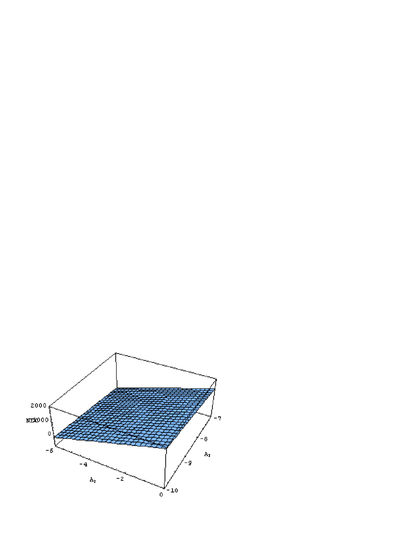
In these cases, one can plot the function in terms of two of the parameters, fixing the other. Despite knowing the sign of the considered parameters with what respect the function may be plotted, the important here is their rank, i.e. the interval to which they must belong in order to produce the positivity of the function. Some examples are presented in Fig. 1.

\bullet The WEC

This condition is realized when the NEC is, plus the condition ρeff0subscript𝜌𝑒𝑓𝑓0\rho_{eff}\geq 0. Note that the complete expression and condition of the NEC read

2n(ΛB2B1)ρn+ρn+1+2B2ρn+1+B22ρ0,forn>0,formulae-sequence2𝑛Λsubscript𝐵2subscript𝐵1superscript𝜌𝑛superscript𝜌𝑛12subscript𝐵2superscript𝜌𝑛1superscriptsubscript𝐵22𝜌0for𝑛0\displaystyle 2n\left(\Lambda B_{2}-B_{1}\right)\rho^{n}+\rho^{n+1}+2B_{2}\rho^{n+1}+B_{2}^{2}\rho\geq 0\,\,,\quad\mbox{for}\quad n>0\,\,, (40)
2n(A1A2Λ)ρn+A22ρn+1+2A2ρn+1+ρ0,forn<0.formulae-sequence2𝑛subscript𝐴1subscript𝐴2Λsuperscript𝜌𝑛superscriptsubscript𝐴22superscript𝜌𝑛12subscript𝐴2superscript𝜌𝑛1𝜌0for𝑛0\displaystyle 2n\left(A_{1}-A_{2}\Lambda\right)\rho^{n}+A_{2}^{2}\rho^{n+1}+2A_{2}\rho^{n+1}+\rho\geq 0\,\,,\quad\mbox{for}\quad n<0\,. (41)

These expressions are obtained by multiplying the numerators in (39) by ρ𝜌\rho. We didn’t need to use this complete expression for determining the conditions on the input parameters in the case of the NEC, since the ordinary energy density is assumed as positive quantity. Besides to (40)-(41), the second condition for satisfying the WEC is

ρeff=ρ+2ρfρ+f(ρ)0,subscript𝜌𝑒𝑓𝑓𝜌2𝜌subscript𝑓𝜌𝑓𝜌0\displaystyle\rho_{eff}=\rho+2\rho f_{\rho}+f(\rho)\geq 0\quad, (42)

having in mind that the ordinary content is assumed as pressureless. By using f(ρ)𝑓𝜌f(\rho) according to the functions in (36), (42) becomes

Λρ2n+ρ2n+1+2B2ρn+1+(2nΛB22nB1+ΛB2+B1)ρn+B22ρ+B1B20,forn>0,formulae-sequenceΛsuperscript𝜌2𝑛superscript𝜌2𝑛12subscript𝐵2superscript𝜌𝑛12𝑛Λsubscript𝐵22𝑛subscript𝐵1Λsubscript𝐵2subscript𝐵1superscript𝜌𝑛superscriptsubscript𝐵22𝜌subscript𝐵1subscript𝐵20for𝑛0\displaystyle\Lambda\rho^{2n}+\rho^{2n+1}+2B_{2}\rho^{n+1}+\left(2n\Lambda B_{2}-2nB_{1}+\Lambda B_{2}+B_{1}\right)\rho^{n}+B_{2}^{2}\rho+B_{1}B_{2}\geq 0\,\,,\mbox{for}\;\;n>0, (43)
A1A2ρ2n+A22ρ2n+1+2A2ρn+1+(2nA12nA2Λ+A1+ΛA2)ρn+ρ+Λ0,forn<0.formulae-sequencesubscript𝐴1subscript𝐴2superscript𝜌2𝑛superscriptsubscript𝐴22superscript𝜌2𝑛12subscript𝐴2superscript𝜌𝑛12𝑛subscript𝐴12𝑛subscript𝐴2Λsubscript𝐴1Λsubscript𝐴2superscript𝜌𝑛𝜌Λ0for𝑛0\displaystyle A_{1}A_{2}\rho^{2n}+A_{2}^{2}\rho^{2n+1}+2A_{2}\rho^{n+1}+\left(2nA_{1}-2nA_{2}\Lambda+A_{1}+\Lambda A_{2}\right)\rho^{n}+\rho+\Lambda\geq 0\,\,,\mbox{for}\;\;n<0. (44)

Note here that we just use the numerator of the fractions whose the denominators are always positives. By combining (40) with (43)-(44), one gets for the WEC

Λρ2n+2ρ2n+1+4B2ρn+1+2B22ρ+[(1+4n)ΛB2+(14n)B1]ρn+B1B20,forn>0,formulae-sequenceΛsuperscript𝜌2𝑛2superscript𝜌2𝑛14subscript𝐵2superscript𝜌𝑛12subscriptsuperscript𝐵22𝜌delimited-[]14𝑛Λsubscript𝐵214𝑛subscript𝐵1superscript𝜌𝑛subscript𝐵1subscript𝐵20for𝑛0\displaystyle\Lambda\rho^{2n}+2\rho^{2n+1}+4B_{2}\rho^{n+1}+2B^{2}_{2}\rho+\left[(1+4n)\Lambda B_{2}+(1-4n)B_{1}\right]\rho^{n}+B_{1}B_{2}\geq 0,\;\;\mbox{for}\;\;n>0\,, (45)
A1A2ρ2n+2ρ2n+1+4A2ρn+1+2ρ+[(1+4n)A1+(14n)A2Λ]ρn+Λ0,forn<0.formulae-sequencesubscript𝐴1subscript𝐴2superscript𝜌2𝑛2superscript𝜌2𝑛14subscript𝐴2superscript𝜌𝑛12𝜌delimited-[]14𝑛subscript𝐴114𝑛subscript𝐴2Λsuperscript𝜌𝑛Λ0for𝑛0\displaystyle A_{1}A_{2}\rho^{2n}+2\rho^{2n+1}+4A_{2}\rho^{n+1}+2\rho+\left[(1+4n)A_{1}+(1-4n)A_{2}\Lambda\right]\rho^{n}+\Lambda\geq 0,\;\;\mbox{for}\;\;n<0\,\,\,. (46)

We address here the evident conditions for which the WEC is satisfied as follows:

\ast B1>0subscript𝐵10B_{1}>0,  B2>0subscript𝐵20B_{2}>0 for  0<n<1/40𝑛140<n<1/4   ,

\ast A1>0subscript𝐴10A_{1}>0, A2>0subscript𝐴20A_{2}>0,  for  1/4<n<014𝑛0-1/4<n<0   .

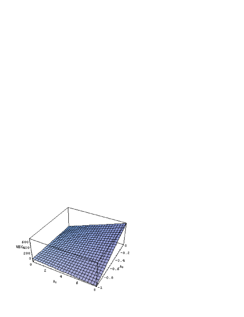
It is obvious that these conditions are not unique. For n>0𝑛0n>0 (n<0𝑛0n<0), the necessity of plotting the function Λρ2n+2ρ2n+1+4B2ρn+1+2B22ρ+[(1+4n)ΛB2+(14n)B1]ρn+B1B2Λsuperscript𝜌2𝑛2superscript𝜌2𝑛14subscript𝐵2superscript𝜌𝑛12subscriptsuperscript𝐵22𝜌delimited-[]14𝑛Λsubscript𝐵214𝑛subscript𝐵1superscript𝜌𝑛subscript𝐵1subscript𝐵2\Lambda\rho^{2n}+2\rho^{2n+1}+4B_{2}\rho^{n+1}+2B^{2}_{2}\rho+\left[(1+4n)\Lambda B_{2}+(1-4n)B_{1}\right]\rho^{n}+B_{1}B_{2},    (A1A2ρ2n+2A22ρ2n+1+4A2ρn+1+2ρ+[(1+4n)A1+(14n)A2Λ]ρn+Λsubscript𝐴1subscript𝐴2superscript𝜌2𝑛2subscriptsuperscript𝐴22superscript𝜌2𝑛14subscript𝐴2superscript𝜌𝑛12𝜌delimited-[]14𝑛subscript𝐴114𝑛subscript𝐴2Λsuperscript𝜌𝑛ΛA_{1}A_{2}\rho^{2n}+2A^{2}_{2}\rho^{2n+1}+4A_{2}\rho^{n+1}+2\rho+\left[(1+4n)A_{1}+(1-4n)A_{2}\Lambda\right]\rho^{n}+\Lambda) varying two of the input parameters and fixing the other, appears when at least one of the following expressions is negative, (B2subscript𝐵2B_{2}, B1B2subscript𝐵1subscript𝐵2B_{1}B_{2} or (1+4n)ΛB2+(14n)B114𝑛Λsubscript𝐵214𝑛subscript𝐵1(1+4n)\Lambda B_{2}+(1-4n)B_{1}),   (A1A2subscript𝐴1subscript𝐴2A_{1}A_{2}, A2subscript𝐴2A_{2}, or (1+4n)A1+(14n)A2Λ14𝑛subscript𝐴114𝑛subscript𝐴2Λ(1+4n)A_{1}+(1-4n)A_{2}\Lambda). We present some examples of theses cases in Fig. 2.

\bullet The SEC

The strong energy condition is realized by combining the NEC with ρeff+3peff0subscript𝜌𝑒𝑓𝑓3subscript𝑝𝑒𝑓𝑓0\rho_{eff}+3p_{eff}\geq 0. This latter reads,

ρeff+3peff=ρ+2ρfρ2f(ρ)0.subscript𝜌𝑒𝑓𝑓3subscript𝑝𝑒𝑓𝑓𝜌2𝜌subscript𝑓𝜌2𝑓𝜌0\displaystyle\rho_{eff}+3p_{eff}=\rho+2\rho f_{\rho}-2f(\rho)\geq 0\quad. (47)

Making use of the expressions in (6), one obtains a fraction whose the denominator is always positive and the numerator reads

ρ2n+1+2B2ρn+1+B22ρ2[(1n)ΛB2+(1+n)B1]ρn2Λρ2n2B1B20,forn>0,formulae-sequencesuperscript𝜌2𝑛12subscript𝐵2superscript𝜌𝑛1superscriptsubscript𝐵22𝜌2delimited-[]1𝑛Λsubscript𝐵21𝑛subscript𝐵1superscript𝜌𝑛2Λsuperscript𝜌2𝑛2subscript𝐵1subscript𝐵20for𝑛0\displaystyle\rho^{2n+1}+2B_{2}\rho^{n+1}+B_{2}^{2}\rho-2\left[(1-n)\Lambda B_{2}+(1+n)B_{1}\right]\rho^{n}-2\Lambda\rho^{2n}-2B_{1}B_{2}\geq 0\,,\mbox{for}\;n>0\,\,, (48)
A22ρ2n+1+2A2ρn+1+ρ2[(1n)A1+(1+n)A2Λ]ρn2A1A2ρ2n2Λ0forn<0.superscriptsubscript𝐴22superscript𝜌2𝑛12subscript𝐴2superscript𝜌𝑛1𝜌2delimited-[]1𝑛subscript𝐴11𝑛subscript𝐴2Λsuperscript𝜌𝑛2subscript𝐴1subscript𝐴2superscript𝜌2𝑛2Λ0for𝑛0\displaystyle A_{2}^{2}\rho^{2n+1}+2A_{2}\rho^{n+1}+\rho-2\left[(1-n)A_{1}+(1+n)A_{2}\Lambda\right]\rho^{n}-2A_{1}A_{2}\rho^{2n}-2\Lambda\geq 0\,\mbox{for}\;n<0\,\,. (49)

Now, combining (48)-(49) with the NEC, on gets the following conditions for the SEC

2ρ2n+12Λρ2n+4B2ρn+1+2B22ρ2[(12n)ΛB2+(1+2n)B1]ρn2B1B20,forn>0,formulae-sequence2superscript𝜌2𝑛12Λsuperscript𝜌2𝑛4subscript𝐵2superscript𝜌𝑛12subscriptsuperscript𝐵22𝜌2delimited-[]12𝑛Λsubscript𝐵212𝑛subscript𝐵1superscript𝜌𝑛2subscript𝐵1subscript𝐵20for𝑛0\displaystyle 2\rho^{2n+1}-2\Lambda\rho^{2n}+4B_{2}\rho^{n+1}+2B^{2}_{2}\rho-2\left[(1-2n)\Lambda B_{2}+(1+2n)B_{1}\right]\rho^{n}-2B_{1}B_{2}\geq 0\,,\;\mbox{for}\;n>0\,, (50)
2A22ρ2n+12A1A2ρ2n+4A2ρn+1+2ρ2[(12n)A1+(1+2n)A2Λ]ρn2Λ0,forn<0.formulae-sequence2superscriptsubscript𝐴22superscript𝜌2𝑛12subscript𝐴1subscript𝐴2superscript𝜌2𝑛4subscript𝐴2superscript𝜌𝑛12𝜌2delimited-[]12𝑛subscript𝐴112𝑛subscript𝐴2Λsuperscript𝜌𝑛2Λ0for𝑛0\displaystyle 2A_{2}^{2}\rho^{2n+1}-2A_{1}A_{2}\rho^{2n}+4A_{2}\rho^{n+1}+2\rho-2\left[(1-2n)A_{1}+(1+2n)A_{2}\Lambda\right]\rho^{n}-2\Lambda\geq 0\,,\;\mbox{for}\;n<0\,. (51)

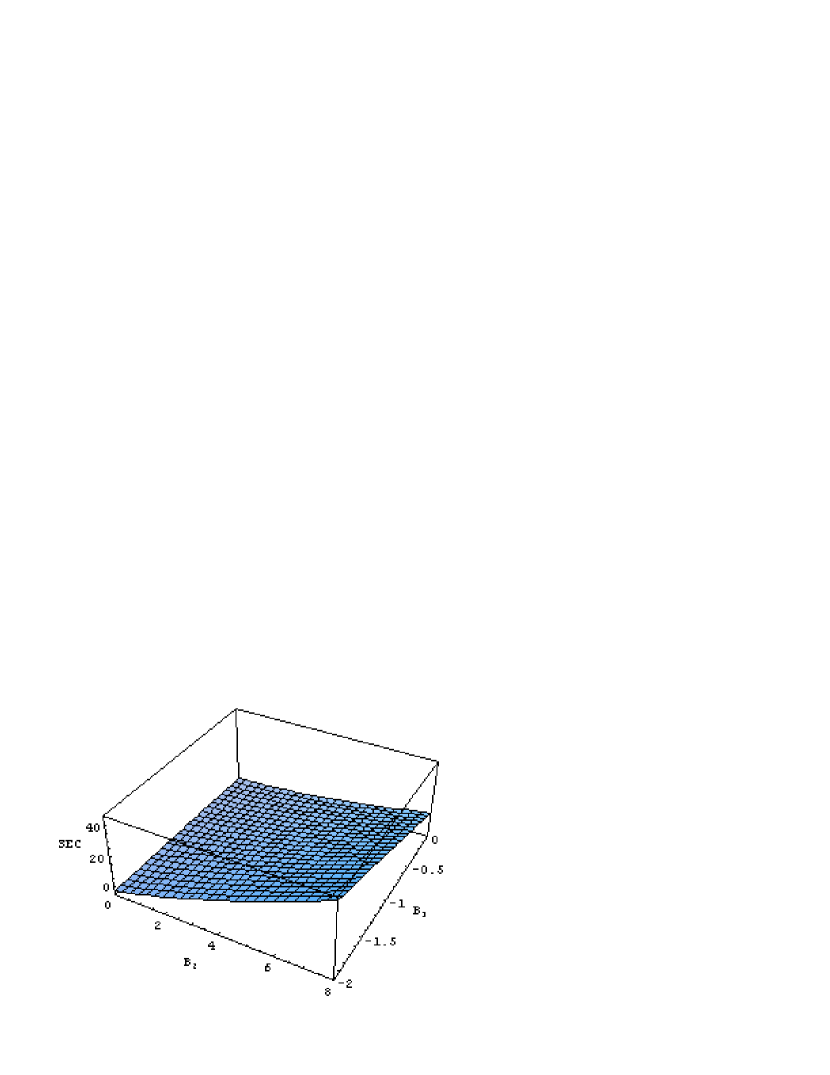
In this case, there is any obvious condition for satisfying the SEC. However, values can be found, by plotting 2ρ2n+12Λρ2n+4B2ρn+1+2B22ρ2[(12n)ΛB2+(1+2n)B1]ρn2B1B22superscript𝜌2𝑛12Λsuperscript𝜌2𝑛4subscript𝐵2superscript𝜌𝑛12subscriptsuperscript𝐵22𝜌2delimited-[]12𝑛Λsubscript𝐵212𝑛subscript𝐵1superscript𝜌𝑛2subscript𝐵1subscript𝐵22\rho^{2n+1}-2\Lambda\rho^{2n}+4B_{2}\rho^{n+1}+2B^{2}_{2}\rho-2\left[(1-2n)\Lambda B_{2}+(1+2n)B_{1}\right]\rho^{n}-2B_{1}B_{2}  and  2A22ρ2n+12A1A2ρ2n+4A2ρn+1+2ρ2[(12n)A1+(1+2n)A2Λ]ρn2Λ2superscriptsubscript𝐴22superscript𝜌2𝑛12subscript𝐴1subscript𝐴2superscript𝜌2𝑛4subscript𝐴2superscript𝜌𝑛12𝜌2delimited-[]12𝑛subscript𝐴112𝑛subscript𝐴2Λsuperscript𝜌𝑛2Λ2A_{2}^{2}\rho^{2n+1}-2A_{1}A_{2}\rho^{2n}+4A_{2}\rho^{n+1}+2\rho-2\left[(1-2n)A_{1}+(1+2n)A_{2}\Lambda\right]\rho^{n}-2\Lambda in terms of two of the parameters. Some examples for illustrating some of these cases are presented in Fig. 3.

\bullet The DEC

The dominant energy condition is characterized by the WEC combined with ρeffpeff0subscript𝜌𝑒𝑓𝑓subscript𝑝𝑒𝑓𝑓0\rho_{eff}-p_{eff}\geq 0. Following the same steps as in the previous cases, one easily obtains the DEC as

ρ2n+1+Λρ2n+2B2ρn+1+B22ρ+B1B2+[(2n+1)ΛB2+(12n)B1]ρn0forn>0,superscript𝜌2𝑛1Λsuperscript𝜌2𝑛2subscript𝐵2superscript𝜌𝑛1superscriptsubscript𝐵22𝜌subscript𝐵1subscript𝐵2delimited-[]2𝑛1Λsubscript𝐵212𝑛subscript𝐵1superscript𝜌𝑛0for𝑛0\displaystyle\rho^{2n+1}+\Lambda\rho^{2n}+2B_{2}\rho^{n+1}+B_{2}^{2}\rho+B_{1}B_{2}+\left[(2n+1)\Lambda B_{2}+(1-2n)B_{1}\right]\rho^{n}\geq 0\,\mbox{for}\;n>0\,\,, (52)
A22ρ2n+1+A1A2ρ2n+2A2ρn+1+ρ+Λ+[(2n+1)A1+(12n)ΛA2]ρn0forn<0.subscriptsuperscript𝐴22superscript𝜌2𝑛1subscript𝐴1subscript𝐴2superscript𝜌2𝑛2subscript𝐴2superscript𝜌𝑛1𝜌Λdelimited-[]2𝑛1subscript𝐴112𝑛Λsubscript𝐴2superscript𝜌𝑛0for𝑛0\displaystyle A^{2}_{2}\rho^{2n+1}+A_{1}A_{2}\rho^{2n}+2A_{2}\rho^{n+1}+\rho+\Lambda+\left[(2n+1)A_{1}+(1-2n)\Lambda A_{2}\right]\rho^{n}\geq 0\,\mbox{for}\;n<0\,\,. (53)

The evident conditions read

\ast B1>0subscript𝐵10B_{1}>0,  B2>0subscript𝐵20B_{2}>0 and  n>1/2𝑛12n>1/2  .

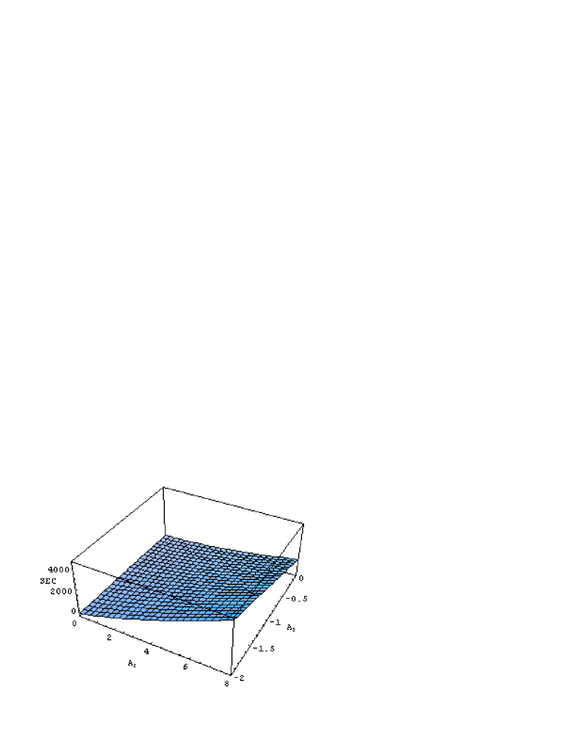
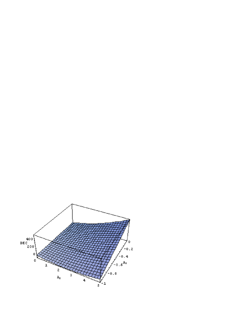
Evidently, other conditions may lead to the accomplishment of the DEC, but, only plotting the functions in (52)-(53). This can occur when at least one of the following expressions is negative,  B2subscript𝐵2B_{2},  B1B2subscript𝐵1subscript𝐵2B_{1}B_{2},  (2n+1)ΛB2+(12n)B12𝑛1Λsubscript𝐵212𝑛subscript𝐵1(2n+1)\Lambda B_{2}+(1-2n)B_{1} for (52). We recall that the negative parameters must be suitably chosen without loosing the positivity of the expressions (52)-(53). We present some of theses cases in Fig. 4.

4.2 Studying the case f(T)=a3lnq(b3Tm)𝑓𝑇subscript𝑎3superscript𝑞subscript𝑏3superscript𝑇𝑚f(T)=a_{3}\ln^{q}{\left(b_{3}T^{m}\right)}

Here we will work with the fundamental conditions for which the model allows the avoidance of the Big Rip. So, we propose to check if the range of parameters for which the singularity may be cured can also make the model satisfying the energy conditions. Here, the first derivative of f(ρ)𝑓𝜌f(\rho) also plays an important role. Deriving f(ρ)𝑓𝜌f(\rho) with respect to the energy density ρ𝜌\rho, one gets

fρ(ρ)=qma3ρlnq1(b3ρm).subscript𝑓𝜌𝜌𝑞𝑚subscript𝑎3𝜌superscript𝑞1subscript𝑏3superscript𝜌𝑚\displaystyle f_{\rho}(\rho)=\frac{qma_{3}}{\rho}\ln^{q-1}{\left(b_{3}\rho^{m}\right)}\quad. (54)

We believe that each step of constructing the four energy conditions is now clear and we simply present the results and comments as follows:

\bullet NEC

ρ+2qma3+ρlnq1(b3ρm)0.𝜌2𝑞𝑚subscript𝑎3𝜌superscript𝑞1subscript𝑏3superscript𝜌𝑚0\displaystyle\rho+2qma_{3}+\rho\ln^{q-1}{\left(b_{3}\rho^{m}\right)}\geq 0\,\,\,\,. (55)

The evident conditions for obtaining this are

\ast q>0𝑞0q>0,  m<0𝑚0m<0,  a3<0subscript𝑎30a_{3}<0, with ρm>1/b3superscript𝜌𝑚1subscript𝑏3\rho^{m}>1/b_{3}    .

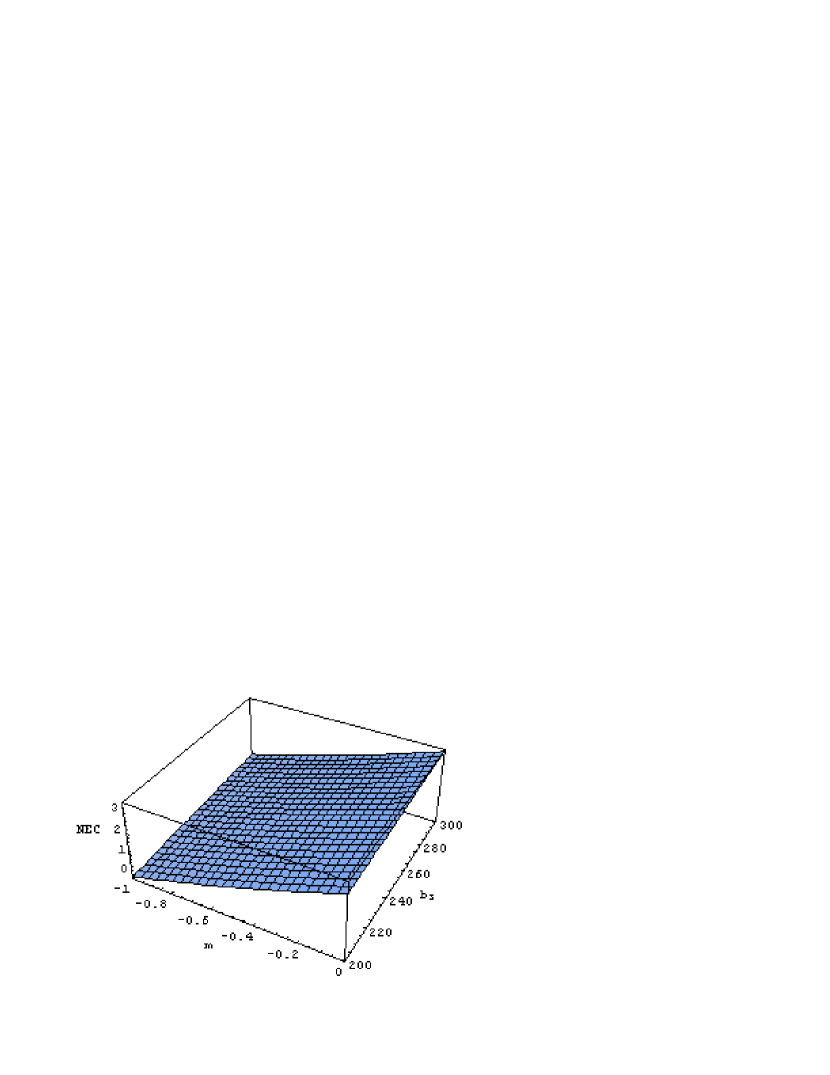
It is important to note that this list is not exhaustive, since in other conditions different from the above ones, the NEC could still be realized. This is a set of the situations where for example 2qma3<02𝑞𝑚subscript𝑎302qma_{3}<0, but its absolute value is less than the absolute value of ρ+ρlnq1(b3ρm)𝜌𝜌superscript𝑞1subscript𝑏3superscript𝜌𝑚\rho+\rho\ln^{q-1}{(b_{3}\rho^{m})}, i.e., |2qma3|<|ρ+ρlnq1(b3ρm)|2𝑞𝑚subscript𝑎3𝜌𝜌superscript𝑞1subscript𝑏3superscript𝜌𝑚|2qma_{3}|<|\rho+\rho\ln^{q-1}{(b_{3}\rho^{m})}|. This situation requires knowing some intervals to which the parameters must belong. We present this feature by plotting the function corresponding to the expression (55) in terms of some of the input parameters fixing the other. See the graph at left side in Fig. 5.

\bullet WEC

2ρ+2qma3+(ρ+2qma3)lnq1(b3ρm)+a3lnq(b3ρm)0.2𝜌2𝑞𝑚subscript𝑎3𝜌2𝑞𝑚subscript𝑎3superscript𝑞1subscript𝑏3superscript𝜌𝑚subscript𝑎3superscript𝑞subscript𝑏3superscript𝜌𝑚0\displaystyle 2\rho+2qma_{3}+\left(\rho+2qma_{3}\right)\ln^{q-1}{\left(b_{3}\rho^{m}\right)}+a_{3}\ln^{q}{\left(b_{3}\rho^{m}\right)}\geq 0\,\,\,\,. (56)

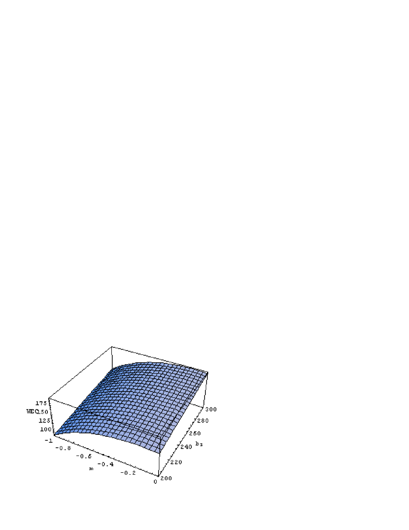
In this case by plotting the function (56), the WEC can be realized graphically. This is the set of situations where one of the term in the sum (56) is negative, but it absolute value is less that the absolute value of the sum of the other. An example for this is when 2qma3<02𝑞𝑚subscript𝑎302qma_{3}<0, but |2qma3|<2ρ+|(ρ+2qma3)lnq1(b3ρm)+a3lnq(b3ρm)|2𝑞𝑚subscript𝑎32𝜌𝜌2𝑞𝑚subscript𝑎3superscript𝑞1subscript𝑏3superscript𝜌𝑚subscript𝑎3superscript𝑞subscript𝑏3superscript𝜌𝑚|2qma_{3}|<2\rho+|\left(\rho+2qma_{3}\right)\ln^{q-1}{\left(b_{3}\rho^{m}\right)}+a_{3}\ln^{q}{\left(b_{3}\rho^{m}\right)}|. See the graph at right side in Fig. 5.

\bullet SEC

2ρ+2qma3+(ρ+2qma3)lnq1(b3ρm)2a3lnq(b3ρm)0.2𝜌2𝑞𝑚subscript𝑎3𝜌2𝑞𝑚subscript𝑎3superscript𝑞1subscript𝑏3superscript𝜌𝑚2subscript𝑎3superscript𝑞subscript𝑏3superscript𝜌𝑚0\displaystyle 2\rho+2qma_{3}+\left(\rho+2qma_{3}\right)\ln^{q-1}{\left(b_{3}\rho^{m}\right)}-2a_{3}\ln^{q}{\left(b_{3}\rho^{m}\right)}\geq 0\,\,\,. (57)

In this case, evident constraints on the input parameters in order to realize this energy conditions are presented as follows:

\ast q>0𝑞0q>0,  m<0𝑚0m<0,  a3<0subscript𝑎30a_{3}<0, with ρm>1/b3superscript𝜌𝑚1subscript𝑏3\rho^{m}>1/b_{3}    ,

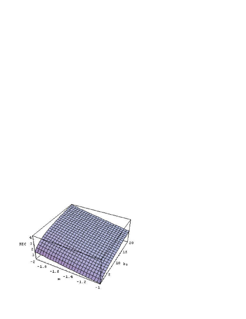
As presented in the previous cases, other conditions may also realize this energy conditions. This can be observed by plotting the function in (57) in terms of some input parameters, fixing the other. See the graph at left side in Fig. 6.

\bullet DEC

3ρ+2qma3+(ρ+4qma3)lnq1(b3ρm)+3a3lnq(b3ρm)0.3𝜌2𝑞𝑚subscript𝑎3𝜌4𝑞𝑚subscript𝑎3superscript𝑞1subscript𝑏3superscript𝜌𝑚3subscript𝑎3superscript𝑞subscript𝑏3superscript𝜌𝑚0\displaystyle 3\rho+2qma_{3}+\left(\rho+4qma_{3}\right)\ln^{q-1}{\left(b_{3}\rho^{m}\right)}+3a_{3}\ln^{q}{\left(b_{3}\rho^{m}\right)}\geq 0\,\,\,. (58)

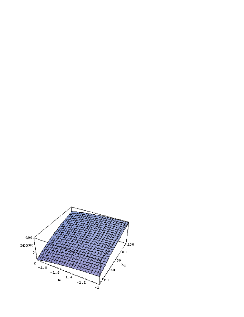
Here, constraints may also lead to the DEC, but this is clear by plotting the function (58), as in the previous cases. We present an illustrative example at right side in Fig. 6.

We mention that for all the graphs, the parameters are normalised to 10121superscript1012110^{-121} Planck units. Remark that the current value of the cosmological constant is about 1.7×101211.7superscript101211.7\times 10^{-121} and the energy density of the usual matter is about ρ=0.1×10121𝜌0.1superscript10121\rho=0.1\times 10^{-121} [14]. Then, with the normalization, we get Λ=1.7Λ1.7\Lambda=1.7 and ρ=0.1𝜌0.1\rho=0.1 for the cosmological constant and the energy density of the usual matter respectively, which are the values used for plotting the graph in the figures. Moreover, we observe that all the conditions which lead to the accomplishment of the NEC also satisfy the WEC, the SEC and the DEC. This is an obvious deduction from (29)-(32). In the same way, it is easy to observe that all the conditions for which the WEC is satisfied, also lead to the accomplishment of the DEC. From the same expressions (30)-(31), we see that the sufficient condition for the requirement of satisfying the WEC leads to the accomplishment of the SEC is f(T)<0𝑓𝑇0f(T)<0. Thus, among the conditions for which the WEC is satisfied, those for which the function is always negative, also lead to the accomplishment of the SEC. However, about the SEC with respect to the DEC, the situation is quite different. The requirement for, the conditions which satisfy the SEC, leading to the accomplishment of the DEC, is always having f(T)>0𝑓𝑇0f(T)>0. This means that, among the conditions for which the SEC is satisfied, those for which the function f(T)𝑓𝑇f(T) is always positive, guarantee the accomplishment of the DEC.

5 Perturbations and stabilities in R+2f(T)𝑅2𝑓𝑇R+2f(T) gravity

In this section we propose to study the perturbations around the models used in this work. We can start establishing the perturbed equations for the case R+2f(T)𝑅2𝑓𝑇R+2f(T), but the two models will be studied as specific cases.

For this purpose, let us assume a general solution for the cosmological background of FRW metric, which is given by a Hubble parameter H=Hb(t)𝐻subscript𝐻𝑏𝑡H=H_{b}(t) that satisfies the background equation (27) using (25), for R+2f(T)𝑅2𝑓𝑇R+2f(T) gravity. The evolution of the matter energy density can be expressed in terms of this particular solution by solving the continuity equation around Hb(t)subscript𝐻𝑏𝑡H_{b}(t),

ρ˙b+3Hb(t)ρb=0,subscript˙𝜌𝑏3subscript𝐻𝑏𝑡subscript𝜌𝑏0\displaystyle\dot{\rho}_{b}+3H_{b}(t)\rho_{b}=0\,\,\,, (59)

yielding

ρb(t)=ρ0e3Hb(t)𝑑t.subscript𝜌𝑏𝑡subscript𝜌0superscript𝑒3subscript𝐻𝑏𝑡differential-d𝑡\displaystyle\rho_{b}(t)=\rho_{0}e^{-3\int H_{b}(t)dt}\,\,\,\,. (60)

We recall that we are considering that the ordinary content of the universe is pressureless. Since we are interesting in studying the perturbations around the solutions H=Hb(t)𝐻subscript𝐻𝑏𝑡H=H_{b}(t), we will consider small deviations from the Hubble parameter and the energy density, i.e., we can write the Hubble parameter and the ordinary energy density as [23]

H(t)=Hb(t)(1+δ(t)),ρ(t)=ρb(t)(1+δm(t)).formulae-sequence𝐻𝑡subscript𝐻𝑏𝑡1𝛿𝑡𝜌𝑡subscript𝜌𝑏𝑡1subscript𝛿𝑚𝑡\displaystyle H(t)=H_{b}(t)\left(1+\delta(t)\right)\,\,\,,\quad\rho(t)=\rho_{b}(t)\left(1+\delta_{m}(t)\right)\,\,\,. (61)

In order to study the behaviour of these perturbations in the linear regime, we expand the function f(T)𝑓𝑇f(T) in powers of Tbsubscript𝑇𝑏T_{b} (or ρbsubscript𝜌𝑏\rho_{b}) evaluated at the solution H=Hb(t)𝐻subscript𝐻𝑏𝑡H=H_{b}(t), as

f(T)=f(ρ)=fb+fρb(ρρb)+𝒪2,𝑓𝑇𝑓𝜌superscript𝑓𝑏superscriptsubscript𝑓𝜌𝑏𝜌subscript𝜌𝑏superscript𝒪2\displaystyle f(T)=f(\rho)=f^{b}+f_{\rho}^{b}(\rho-\rho_{b})+\mathcal{O}^{2}\,\,\,\,, (62)

where the superscript b𝑏b refers to the background values of f(T)𝑓𝑇f(T) and its derivatives evaluated at T=Tb𝑇subscript𝑇𝑏T=T_{b} (or ρ=ρb𝜌subscript𝜌𝑏\rho=\rho_{b}). Here, the 𝒪𝒪\mathcal{O} term includes all the terms proportional to the square or higher powers of T𝑇T (or ρ𝜌\rho). Then, only the linear terms of the induced perturbations will be considered. Hence, by making use of the expression (61) in the Eqs. (27) and (25), one gets the equation for the perturbation δ(t)𝛿𝑡\delta(t) in the linear approximation,

(ρb+3ρbfρb+2ρb2fρρb)δm(t)=6Hb2δ(t).subscript𝜌𝑏3subscript𝜌𝑏subscriptsuperscript𝑓𝑏𝜌2subscriptsuperscript𝜌2𝑏subscriptsuperscript𝑓𝑏𝜌𝜌subscript𝛿𝑚𝑡6superscriptsubscript𝐻𝑏2𝛿𝑡\displaystyle\left(\rho_{b}+3\rho_{b}f^{b}_{\rho}+2\rho^{2}_{b}f^{b}_{\rho\rho}\right)\delta_{m}(t)=6H_{b}^{2}\delta(t)\,\,\,. (63)

On the other hand, there is a second perturbed equation from the matter continuity equation,

δ˙m+3Hb(t)δ(t)=0.subscript˙𝛿𝑚3subscript𝐻𝑏𝑡𝛿𝑡0\displaystyle\dot{\delta}_{m}+3H_{b}(t)\delta(t)=0\,\,\,. (64)

By combining Eqs. (63) and (64) one gets the following equation for the matter perturbation

2Hbδ˙m+(ρb+3ρbfρb+2ρb2fρρb)δm=0,2subscript𝐻𝑏subscript˙𝛿𝑚subscript𝜌𝑏3subscript𝜌𝑏subscriptsuperscript𝑓𝑏𝜌2subscriptsuperscript𝜌2𝑏subscriptsuperscript𝑓𝑏𝜌𝜌subscript𝛿𝑚0\displaystyle 2H_{b}\dot{\delta}_{m}+\left(\rho_{b}+3\rho_{b}f^{b}_{\rho}+2\rho^{2}_{b}f^{b}_{\rho\rho}\right)\delta_{m}=0\,\,\,, (65)

from which we obtain

δm(t)=C1exp{12Cb𝑑t},Cb=ρbHb(1+3fρb+2ρbfρρb),formulae-sequencesubscript𝛿𝑚𝑡subscript𝐶112subscript𝐶𝑏differential-d𝑡subscript𝐶𝑏subscript𝜌𝑏subscript𝐻𝑏13subscriptsuperscript𝑓𝑏𝜌2subscript𝜌𝑏subscriptsuperscript𝑓𝑏𝜌𝜌\displaystyle\delta_{m}(t)=C_{1}\exp{\left\{-\frac{1}{2}\int C_{b}dt\right\}}\,\,,\quad C_{b}=\frac{\rho_{b}}{H_{b}}\left(1+3f^{b}_{\rho}+2\rho_{b}f^{b}_{\rho\rho}\right)\,\,\,, (66)

where C1subscript𝐶1C_{1} is an integration constant. By using the relation (64), the perturbation δ𝛿\delta reads

δ(t)=C1Cb6Hbexp{12Cb𝑑t}.𝛿𝑡subscript𝐶1subscript𝐶𝑏6subscript𝐻𝑏12subscript𝐶𝑏differential-d𝑡\displaystyle\delta(t)=-\frac{C_{1}C_{b}}{6H_{b}}\exp{\left\{-\frac{1}{2}\int C_{b}dt\right\}}\,\,. (67)

Let us now consider two cosmological solutions and analyse their stability by the use of the models treated in this work: de Sitter solutions and power-law solutions.

5.1 Stability of de Sitter solutions

In de Sitter solutions, the Hubble parameter is constant and one has

Hb(t)=H0,a(t)=a0eH0t,\displaystyle H_{b}(t)=H_{0}\,\,,\rightarrow a(t)=a_{0}e^{H_{0}t}\,\,\,, (68)

where H0subscript𝐻0H_{0} is constant.

With this scale factor, the energy density of the background becomes ρb=ρ0e3H0tsubscript𝜌𝑏subscript𝜌0superscript𝑒3subscript𝐻0𝑡\rho_{b}=\rho_{0}e^{-3H_{0}t}, with which one has dρb=3H0ρbdt𝑑subscript𝜌𝑏3subscript𝐻0subscript𝜌𝑏𝑑𝑡d\rho_{b}=-3H_{0}\rho_{b}dt. By using this, one can cast the integral in (66) into

Cb𝑑t=13H02(1+3fρb+2ρbfρρb)𝑑ρb.subscript𝐶𝑏differential-d𝑡13subscriptsuperscript𝐻2013subscriptsuperscript𝑓𝑏𝜌2subscript𝜌𝑏subscriptsuperscript𝑓𝑏𝜌𝜌differential-dsubscript𝜌𝑏\displaystyle\int C_{b}dt=-\frac{1}{3H^{2}_{0}}\int\left(1+3f^{b}_{\rho}+2\rho_{b}f^{b}_{\rho\rho}\right)d\rho_{b}\,\,\,. (69)

\bullet Treating the model f(T)=ΛTn+B1Tn+B2𝑓𝑇Λsuperscript𝑇𝑛subscript𝐵1superscript𝑇𝑛subscript𝐵2f(T)=\frac{\Lambda T^{n}+B_{1}}{T^{n}+B_{2}}.

This case corresponds to n>0𝑛0n>0, and the integral (69) can be expressed as

Cb𝑑t=13H02[ρbΛB2B1B2+ρbn+2n(ΛB2B1)ρbn(B2+ρbn)2],ρbn=ρ0ne3nH0t,formulae-sequencesubscript𝐶𝑏differential-d𝑡13subscriptsuperscript𝐻20delimited-[]subscript𝜌𝑏Λsubscript𝐵2subscript𝐵1subscript𝐵2subscriptsuperscript𝜌𝑛𝑏2𝑛Λsubscript𝐵2subscript𝐵1superscriptsubscript𝜌𝑏𝑛superscriptsubscript𝐵2superscriptsubscript𝜌𝑏𝑛2superscriptsubscript𝜌𝑏𝑛superscriptsubscript𝜌0𝑛superscript𝑒3𝑛subscript𝐻0𝑡\displaystyle\int C_{b}dt=-\frac{1}{3H^{2}_{0}}\left[\rho_{b}-\frac{\Lambda B_{2}-B_{1}}{B_{2}+\rho^{n}_{b}}+\frac{2n(\Lambda B_{2}-B_{1})\rho_{b}^{n}}{(B_{2}+\rho_{b}^{n})^{2}}\right]\,\,,\quad\rho_{b}^{n}=\rho_{0}^{n}e^{-3nH_{0}t}\,\,\,, (70)

and Cbsubscript𝐶𝑏C_{b} is written as

Cb=1H0[ρb+n(2n+1)(ΛB2B1)ρbn(ρbn+B2)24n2(ΛB2B1)ρb2n(ρbn+B2)3].subscript𝐶𝑏1subscript𝐻0delimited-[]subscript𝜌𝑏𝑛2𝑛1Λsubscript𝐵2subscript𝐵1superscriptsubscript𝜌𝑏𝑛superscriptsuperscriptsubscript𝜌𝑏𝑛subscript𝐵224superscript𝑛2Λsubscript𝐵2subscript𝐵1superscriptsubscript𝜌𝑏2𝑛superscriptsuperscriptsubscript𝜌𝑏𝑛subscript𝐵23\displaystyle C_{b}=\frac{1}{H_{0}}\left[\rho_{b}+\frac{n(2n+1)(\Lambda B_{2}-B_{1})\rho_{b}^{n}}{(\rho_{b}^{n}+B_{2})^{2}}-\frac{4n^{2}(\Lambda B_{2}-B_{1})\rho_{b}^{2n}}{(\rho_{b}^{n}+B_{2})^{3}}\right]\,\,. (71)

We see from (70) and (71) that for n>0𝑛0n>0, and as the time evolves, the stability of de Sitter solutions requires B20subscript𝐵20B_{2}\neq 0. In other word, for the initial model f(T)=a1Tn+b1a2Tn+b2𝑓𝑇subscript𝑎1superscript𝑇𝑛subscript𝑏1subscript𝑎2superscript𝑇𝑛subscript𝑏2f(T)=\frac{a_{1}T^{n}+b_{1}}{a_{2}T^{n}+b_{2}}, de Sitter solutions are stables if and only if a20subscript𝑎20a_{2}\neq 0 and b20subscript𝑏20b_{2}\neq 0.

\bullet Treating the model f(T)=A1Tn+ΛA2Tn+1𝑓𝑇subscript𝐴1superscript𝑇𝑛Λsubscript𝐴2superscript𝑇𝑛1f(T)=\frac{A_{1}T^{n}+\Lambda}{A_{2}T^{n}+1}.

This case corresponds to n<0𝑛0n<0, and the integral (69), multiplied by 1/212-1/2, can be expressed as

12Cb𝑑t=16H02[ρbA1ΛA2A2(1+A2ρbn)+2n(A1ΛA2)ρbn(1+A2ρbn)2],ρbn=ρ0ne3nH0t,formulae-sequence12subscript𝐶𝑏differential-d𝑡16subscriptsuperscript𝐻20delimited-[]subscript𝜌𝑏subscript𝐴1Λsubscript𝐴2subscript𝐴21subscript𝐴2subscriptsuperscript𝜌𝑛𝑏2𝑛subscript𝐴1Λsubscript𝐴2superscriptsubscript𝜌𝑏𝑛superscript1subscript𝐴2superscriptsubscript𝜌𝑏𝑛2superscriptsubscript𝜌𝑏𝑛superscriptsubscript𝜌0𝑛superscript𝑒3𝑛subscript𝐻0𝑡\displaystyle-\frac{1}{2}\int C_{b}dt=\frac{1}{6H^{2}_{0}}\left[\rho_{b}-\frac{A_{1}-\Lambda A_{2}}{A_{2}(1+A_{2}\rho^{n}_{b})}+\frac{2n(A_{1}-\Lambda A_{2})\rho_{b}^{n}}{(1+A_{2}\rho_{b}^{n})^{2}}\right]\,\,,\quad\rho_{b}^{n}=\rho_{0}^{n}e^{-3nH_{0}t}\,\,\,, (72)

and Cbsubscript𝐶𝑏C_{b} is written as

Cb=1H0[ρb+n(2n+1)(A1ΛA2)ρbn(A2ρbn+1)24n2A2(A1ΛA2)ρb2n(A2ρbn+1)3].subscript𝐶𝑏1subscript𝐻0delimited-[]subscript𝜌𝑏𝑛2𝑛1subscript𝐴1Λsubscript𝐴2superscriptsubscript𝜌𝑏𝑛superscriptsubscript𝐴2superscriptsubscript𝜌𝑏𝑛124superscript𝑛2subscript𝐴2subscript𝐴1Λsubscript𝐴2superscriptsubscript𝜌𝑏2𝑛superscriptsubscript𝐴2superscriptsubscript𝜌𝑏𝑛13\displaystyle C_{b}=\frac{1}{H_{0}}\left[\rho_{b}+\frac{n(2n+1)(A_{1}-\Lambda A_{2})\rho_{b}^{n}}{(A_{2}\rho_{b}^{n}+1)^{2}}-\frac{4n^{2}A_{2}(A_{1}-\Lambda A_{2})\rho_{b}^{2n}}{(A_{2}\rho_{b}^{n}+1)^{3}}\right]\,\,. (73)

Here, for n<0𝑛0n<0, as the time evolves, both (72) and (73) tend to ++\infty. Thus the perturbation will grow exponentially, and this particular de Sitter solution becomes unstable. Note that this result does not depend on any of the parameters A1subscript𝐴1A_{1} or A2subscript𝐴2A_{2}.

\bullet Treating the model f(T)=a3lnq(b3Tm)𝑓𝑇subscript𝑎3superscript𝑞subscript𝑏3superscript𝑇𝑚f(T)=a_{3}\ln^{q}{\left(b_{3}T^{m}\right)}.

With this model, the integral (69), multiplied by 1/212-1/2, can be performed and one gets

12Cb𝑑t=16H0[ρb+a3lnq(b3ρm)+2mqa3lnq1(b3ρm)],12subscript𝐶𝑏differential-d𝑡16subscript𝐻0delimited-[]subscript𝜌𝑏subscript𝑎3superscript𝑞subscript𝑏3superscript𝜌𝑚2𝑚𝑞subscript𝑎3superscript𝑞1subscript𝑏3superscript𝜌𝑚\displaystyle-\frac{1}{2}\int C_{b}dt=\frac{1}{6H_{0}}\left[\rho_{b}+a_{3}\ln^{q}{\left(b_{3}\rho^{m}\right)}+2mqa_{3}\ln^{q-1}{\left(b_{3}\rho^{m}\right)}\right]\,\,\,, (74)

with the corresponding expression of Cbsubscript𝐶𝑏C_{b} being

Cb=1H0[ρb+qma3lnq1(b3ρm)+2mq(q1)a3lnq2(b3ρm)].subscript𝐶𝑏1subscript𝐻0delimited-[]subscript𝜌𝑏𝑞𝑚subscript𝑎3superscript𝑞1subscript𝑏3superscript𝜌𝑚2𝑚𝑞𝑞1subscript𝑎3superscript𝑞2subscript𝑏3superscript𝜌𝑚\displaystyle C_{b}=\frac{1}{H_{0}}\left[\rho_{b}+qma_{3}\ln^{q-1}{\left(b_{3}\rho^{m}\right)}+2mq(q-1)a_{3}\ln^{q-2}{\left(b_{3}\rho^{m}\right)}\right]\,\,. (75)

Let us recall that this model (f(T)=a3lnq(b3Tm)𝑓𝑇subscript𝑎3superscript𝑞subscript𝑏3superscript𝑇𝑚f(T)=a_{3}\ln^{q}{\left(b_{3}T^{m}\right)}), leads to the avoidance of the Big Rip for q>2α/(α1)𝑞2𝛼𝛼1q>2\alpha/(\alpha-1) and m<0𝑚0m<0, where α>1𝛼1\alpha>1, as we have previously shown. These conditions also allow the model to satisfy the energy conditions. Now, let us check what happens about the stability with these conditions. First, note that the relation q>2α/(α1)𝑞2𝛼𝛼1q>2\alpha/(\alpha-1) can be cast into q>2+2/(α1)𝑞22𝛼1q>2+2/(\alpha-1), showing that q>2𝑞2q>2 because of α>1𝛼1\alpha>1. By choosing a3<0subscript𝑎30a_{3}<0, we see that, within the conditions q>2𝑞2q>2 and m<0𝑚0m<0, the expressions (74) and (75) tend to -\infty as the time evolves, and this ensures the decay of the perturbation, leading to the stability of de Sitter solutions with this model. Thus, regarding to the stability of de Sitter solutions, the energy conditions and the late time acceleration, provided with the conditions a3<0subscript𝑎30a_{3}<0, b3>0subscript𝑏30b_{3}>0, q>2𝑞2q>2 and m<0𝑚0m<0, we can conclude that the model may be cosmologically acceptable.

5.2 Stability of power-law solutions

As we are dealing with dust as ordinary content of the universe, we will be interested to the scale factor

a(t)a0t2/3Hb(t)=2a03t,ρbt2.formulae-sequence𝑎𝑡subscript𝑎0superscript𝑡23subscript𝐻𝑏𝑡2subscript𝑎03𝑡proportional-tosubscript𝜌𝑏superscript𝑡2\displaystyle a(t)a_{0}t^{2/3}\,\,\,\rightarrow\,\,\,H_{b}(t)=\frac{2a_{0}}{3t}\,\,\,,\quad\rho_{b}\propto t^{-2}\,\,\,. (76)

\bullet Treating the model f(T)=ΛTn+B1Tn+B2𝑓𝑇Λsuperscript𝑇𝑛subscript𝐵1superscript𝑇𝑛subscript𝐵2f(T)=\frac{\Lambda T^{n}+B_{1}}{T^{n}+B_{2}}.

In this case, n>0𝑛0n>0, and one can perform the integral

12Cbdt=34a0[ln(t)(3n+4)(ΛB2B1)t2B2(1+B2t2n)+(ΛB2B1)t22B2n(1+B2t2n)2+\displaystyle-\frac{1}{2}\int C_{b}dt=-\frac{3}{4a_{0}}\Big{[}\ln{(t)}-\frac{(3n+4)(\Lambda B_{2}-B_{1})t^{2}}{B_{2}(1+B_{2}t^{2n})}+\frac{(\Lambda B_{2}-B_{1})t^{2}}{2B_{2}n(1+B_{2}t^{2n})^{2}}+
+(4n+7)(ΛB2B1)t22B22F1(1n,1,1+1n;B2t2n)],\displaystyle+\frac{(4n+7)(\Lambda B_{2}-B_{1})t^{2}}{2B_{2}}\,_{2}F_{1}\left(\frac{1}{n},1,1+\frac{1}{n};-B_{2}t^{2n}\right)\Big{]}\,\,\,, (77)

with,

Cb=32a0[1t+2n(n+1)(ΛB2B1)t2n(t2n+B2)24n2(ΛB2B1)t4n(t2n+B2)3],subscript𝐶𝑏32subscript𝑎0delimited-[]1𝑡2𝑛𝑛1Λsubscript𝐵2subscript𝐵1superscript𝑡2𝑛superscriptsuperscript𝑡2𝑛subscript𝐵224superscript𝑛2Λsubscript𝐵2subscript𝐵1superscript𝑡4𝑛superscriptsuperscript𝑡2𝑛subscript𝐵23\displaystyle C_{b}=\frac{3}{2a_{0}}\left[\frac{1}{t}+\frac{2n(n+1)(\Lambda B_{2}-B_{1})t^{-2n}}{(t^{-2n}+B_{2})^{2}}-\frac{4n^{2}(\Lambda B_{2}-B_{1})t^{-4n}}{(t^{-2n}+B_{2})^{3}}\right]\,\,, (78)

where we have set ρ0=1subscript𝜌01\rho_{0}=1, and F12subscriptsubscript𝐹12\,{}_{2}F_{1} is the hypergeometric function defined by

F12(λ1,λ2,λ3;z)=r=0(λ1)r(λ2)r(λ3)rzrr!subscriptsubscript𝐹12subscript𝜆1subscript𝜆2subscript𝜆3𝑧subscriptsuperscript𝑟0subscriptsubscript𝜆1𝑟subscriptsubscript𝜆2𝑟subscriptsubscript𝜆3𝑟superscript𝑧𝑟𝑟\,{}_{2}F_{1}(\lambda_{1},\lambda_{2},\lambda_{3};z)=\sum^{\infty}_{r=0}\frac{(\lambda_{1})_{r}(\lambda_{2})_{r}}{(\lambda_{3})_{r}}\frac{z^{r}}{r!}\,\,\, (79)
(λ)r=λ(λ+1)(λ+2)(λ+r1),(λ)0=1.formulae-sequencesubscript𝜆𝑟𝜆𝜆1𝜆2𝜆𝑟1subscript𝜆01\displaystyle(\lambda)_{r}=\lambda(\lambda+1)(\lambda+2)...(\lambda+r-1)\,\,\,,\quad(\lambda)_{0}=1\,\,. (80)

As the time evolves, conditions are required for guaranteeing the decay of the perturbation. For B2<0subscript𝐵20B_{2}<0, it is necessary to have ΛB2<B1Λsubscript𝐵2subscript𝐵1\Lambda B_{2}<B_{1}, which means that B1subscript𝐵1B_{1} can be positive, or negative but with |ΛB2|>|B1|Λsubscript𝐵2subscript𝐵1|\Lambda B_{2}|>|B_{1}|. In the case where B2>0subscript𝐵20B_{2}>0 one may observe two sub-cases, i.e., for an even r𝑟r, and an odd r𝑟r . For an even r𝑟r, as the time evolves, the necessary condition for guaranteeing the decay of the perturbation is ΛB2>b1Λsubscript𝐵2subscript𝑏1\Lambda B_{2}>b_{1}, meaning that the parameter B1subscript𝐵1B_{1} can be negative, or positive. On the other hand, for an odd r𝑟r, the requirement for getting the decay of the perturbation is ΛB2<B1Λsubscript𝐵2subscript𝐵1\Lambda B_{2}<B_{1}, meaning that B1>0subscript𝐵10B_{1}>0.

\bullet Treating the model f(T)=A1Tn+ΛA2Tn+1𝑓𝑇subscript𝐴1superscript𝑇𝑛Λsubscript𝐴2superscript𝑇𝑛1f(T)=\frac{A_{1}T^{n}+\Lambda}{A_{2}T^{n}+1}.

Here, n<0𝑛0n<0, and the integral can be performed as

12Cbdt=34a0[ln(t)(2n+3)(A1ΛA2)t22(A2+t2n)+n(A1ΛA2)t2(A2+t2n)2\displaystyle-\frac{1}{2}\int C_{b}dt=-\frac{3}{4a_{0}}\Big{[}\ln{(t)}-\frac{(2n+3)(A_{1}-\Lambda A_{2})t^{2}}{2(A_{2}+t^{2n})}+\frac{n(A_{1}-\Lambda A_{2})t^{2}}{(A_{2}+t^{2n})^{2}}
+3t2(A1ΛA2)2A22F1(1n,1,1+1n;t2nA2)],\displaystyle+\frac{3t^{2}(A_{1}-\Lambda A_{2})}{2A_{2}}\,_{2}F_{1}\left(\frac{1}{n},1,1+\frac{1}{n};-\frac{t^{2n}}{A_{2}}\right)\Big{]}\,\,\,, (81)

with

Cb=32a0[n(2n+1)(A1ΛA2)t2n+1(A2t2n+1)24A2n2(A1ΛA2)t4n+1(A2t2n+1)3].subscript𝐶𝑏32subscript𝑎0delimited-[]𝑛2𝑛1subscript𝐴1Λsubscript𝐴2superscript𝑡2𝑛1superscriptsubscript𝐴2superscript𝑡2𝑛124subscript𝐴2superscript𝑛2subscript𝐴1Λsubscript𝐴2superscript𝑡4𝑛1superscriptsubscript𝐴2superscript𝑡2𝑛13\displaystyle C_{b}=\frac{3}{2a_{0}}\Big{[}\frac{n(2n+1)(A_{1}-\Lambda A_{2})t^{-2n+1}}{(A_{2}t^{-2n}+1)^{2}}-\frac{4A_{2}n^{2}(A_{1}-\Lambda A_{2})t^{-4n+1}}{(A_{2}t^{-2n}+1)^{3}}\Big{]}\,\,. (82)

As the time evolves, the argument of the hypergeometric function tends to zero and the hypergeometric function tends to 111. Thus, the dominant term in (81) reads

34a0A22(A2n)(A1ΛA2)t2.34subscript𝑎0subscriptsuperscript𝐴22subscript𝐴2𝑛subscript𝐴1Λsubscript𝐴2superscript𝑡2\displaystyle\frac{3}{4a_{0}A^{2}_{2}}(A_{2}-n)(A_{1}-\Lambda A_{2})t^{2}\,\,\,. (83)

Here, one can distinguish two cases: (A2n>0subscript𝐴2𝑛0A_{2}-n>0 and A1<ΛA2subscript𝐴1Λsubscript𝐴2A_{1}<\Lambda A_{2}) and (A2n<0subscript𝐴2𝑛0A_{2}-n<0 and A1>ΛA2subscript𝐴1Λsubscript𝐴2A_{1}>\Lambda A_{2}). In the first case, one gets A2>nsubscript𝐴2𝑛A_{2}>n meaning that A2subscript𝐴2A_{2} can be positive, or negative but with |A2|<|n|subscript𝐴2𝑛|A_{2}|<|n|. When A2>0subscript𝐴20A_{2}>0, A1subscript𝐴1A_{1} can be positive or negative, due to the relation A1<ΛA2subscript𝐴1Λsubscript𝐴2A_{1}<\Lambda A_{2}, while for A2<0subscript𝐴20A_{2}<0, A1subscript𝐴1A_{1} is necessarily negative. In the second case, one gets A2<nsubscript𝐴2𝑛A_{2}<n, meaning that A2<0subscript𝐴20A_{2}<0, which allows A1subscript𝐴1A_{1} to be positive, due to the relation A1>ΛA2subscript𝐴1Λsubscript𝐴2A_{1}>\Lambda A_{2}.

We observe that some of the conditions for which the stability occurs, are also compatible with some energy conditions. This shows that for some values of the input parameters, acceptable models can be obtained, at least regarding to the energy conditions, the stability, the late time acceleration of the universe and the avoidance of the Big Rip.

\bullet Treating the model f(T)=a3lnq(b3Tm)𝑓𝑇subscript𝑎3superscript𝑞subscript𝑏3superscript𝑇𝑚f(T)=a_{3}\ln^{q}{\left(b_{3}T^{m}\right)}.

As we have done in the previous cases, the integral can be performed, yielding

12Cb=34a0[ln(t)+12a3qb31mmqΓ[q,g(t)m]+a3q(q1)mqb31mΓ[q1,g(t)m]],g(t)=ln(b3t2m).formulae-sequence12subscript𝐶𝑏34subscript𝑎0delimited-[]𝑡12subscript𝑎3𝑞superscriptsubscript𝑏31𝑚superscript𝑚𝑞Γ𝑞𝑔𝑡𝑚subscript𝑎3𝑞𝑞1superscript𝑚𝑞superscriptsubscript𝑏31𝑚Γ𝑞1𝑔𝑡𝑚𝑔𝑡subscript𝑏3superscript𝑡2𝑚\displaystyle-\frac{1}{2}\int C_{b}=-\frac{3}{4a_{0}}\Big{[}\ln{(t)}+\frac{1}{2}a_{3}qb_{3}^{\frac{1}{m}}m^{q}\Gamma[q,\frac{g(t)}{m}]+a_{3}q(q-1)m^{q}b_{3}^{\frac{1}{m}}\Gamma[q-1,\frac{g(t)}{m}]\Big{]}\,\,\,,g(t)=\ln{(b_{3}t^{-2m})}\,\,\,. (84)

with

Cb=32a0[1t+a3qmtlnq1(b3t2m)+2a3q(q1)m2tlnq2(b3t2m)].subscript𝐶𝑏32subscript𝑎0delimited-[]1𝑡subscript𝑎3𝑞𝑚𝑡superscript𝑞1subscript𝑏3superscript𝑡2𝑚2subscript𝑎3𝑞𝑞1superscript𝑚2𝑡superscript𝑞2subscript𝑏3superscript𝑡2𝑚\displaystyle C_{b}=\frac{3}{2a_{0}}\Big{[}\frac{1}{t}+a_{3}qm\,t\ln^{q-1}{(b_{3}t^{-2m})}+2a_{3}q(q-1)m^{2}t\ln^{q-2}{(b_{3}t^{-2m})}\Big{]}\,\,\,. (85)

As we have previously shown, this model cures the Big Rip for q>2𝑞2q>2 and m<0𝑚0m<0. With these conditions, as the time evolves, only the term ln(t)𝑡\ln{(t)} grows. Since 3ln(t)/(4a0)3𝑡4subscript𝑎0-3\ln{(t)}/(4a_{0}) is negative for large value of the time, it is easy to observe that the perturbation decays, and this corresponds to the stability of the power-law solutions with this model. Observe that in this case, the constraints on the parameters q𝑞q and m𝑚m for which all the energy conditions are satisfied, leads to the stability of the power-law solutions. Thus, regarding to the stability, the energy conditions, the late time acceleration of the universe and the avoidance of the Big Rip, we can conclude that this model can be cosmologically acceptable for a30subscript𝑎30a_{3}\neq 0, b3>0subscript𝑏30b_{3}>0, q>2𝑞2q>2 and m<0𝑚0m<0.

6 Discussions

In this work we discussed the viability of an interesting alternative gravitational theory, namely, modified f(R,T)𝑓𝑅𝑇f(R,T) theory of gravity, where R𝑅R is the curvature scalar and T𝑇T the trace of the energy momentum tensor. For our purpose we took the case where the algebraic function f(R, T) is cast into f(R,T)=f1(R)+f2(T)𝑓𝑅𝑇subscript𝑓1𝑅subscript𝑓2𝑇f(R,T)=f_{1}(R)+f_{2}(T), and focused our attention to the assumption f(R)=R𝑓𝑅𝑅f(R)=R and f2(T)=2f(T)subscript𝑓2𝑇2𝑓𝑇f_{2}(T)=2f(T). The aim of the work is to analyse the viability of two models, f(T)=(a1Tn+b1)/(a2Tn+b2)𝑓𝑇subscript𝑎1superscript𝑇𝑛subscript𝑏1subscript𝑎2superscript𝑇𝑛subscript𝑏2f(T)=(a_{1}T^{n}+b_{1})/(a_{2}T^{n}+b_{2}) and f(T)=a3lnq(b3Tm)𝑓𝑇subscript𝑎3superscript𝑞subscript𝑏3superscript𝑇𝑚f(T)=a_{3}\ln^{q}{\left(b_{3}T^{m}\right)}, (where a1subscript𝑎1a_{1}, a2subscript𝑎2a_{2}, b1subscript𝑏1b_{1}, b2subscript𝑏2b_{2}, n𝑛n, a3subscript𝑎3a_{3}, b3subscript𝑏3b_{3}, q𝑞q and m𝑚m are input parameters) by investigating for which range of each parameters, the models satisfy all the energy conditions or some of them. We also assumed that the usual matter content of the universe is pressureless (dust), for which the trace T=ρ𝑇𝜌T=\rho. Depending of having a20subscript𝑎20a_{2}\neq 0 or b20subscript𝑏20b_{2}\neq 0, and according to the fact that the present stage of the universe may be characterized by the ΛΛ\LambdaCDM model, we distinguished two sub-models for the first one. Thus for a20subscript𝑎20a_{2}\neq 0 and n>0𝑛0n>0, the first model reduces into f(ρ)=(Λρn+B1)/(ρn+B2)𝑓𝜌Λsuperscript𝜌𝑛subscript𝐵1superscript𝜌𝑛subscript𝐵2f(\rho)=(\Lambda\rho^{n}+B_{1})/(\rho^{n}+B_{2}), where B1=b1/a2subscript𝐵1subscript𝑏1subscript𝑎2B_{1}=b_{1}/a_{2} and B2=b2/a2subscript𝐵2subscript𝑏2subscript𝑎2B_{2}=b_{2}/a_{2}, while for b20subscript𝑏20b_{2}\neq 0 and n<0𝑛0n<0, the model reduces into f(ρ)=(A1ρn+Λ)/(A2ρn+Λ)𝑓𝜌subscript𝐴1superscript𝜌𝑛Λsubscript𝐴2superscript𝜌𝑛Λf(\rho)=(A_{1}\rho^{n}+\Lambda)/(A_{2}\rho^{n}+\Lambda), where A1=a1/b2subscript𝐴1subscript𝑎1subscript𝑏2A_{1}=a_{1}/b_{2} and A2=a2/b2subscript𝐴2subscript𝑎2subscript𝑏2A_{2}=a_{2}/b_{2}. Energy conditions are generalised to the f(R,T)𝑓𝑅𝑇f(R,T) by acting directly on the effective energy density and pressure, respectively ρeffsubscript𝜌𝑒𝑓𝑓\rho_{eff} and peffsubscript𝑝𝑒𝑓𝑓p_{eff} of the corresponding dark fluid. The same energy conditions, the null, weak, strong and dominant, applied to the ordinary energy density and pressure in GR are then valid for the effective energy density and pressure. Besides to the evident constraints on the input parameters for each of the expressions of f(T)𝑓𝑇f(T), for obtaining R+2f(T)𝑅2𝑓𝑇R+2f(T) gravity models that satisfy energy conditions, we also presented figures characterizing models satisfying energy conditions, and whose parameters cannot be determined analytically, but rather, numerically. For plotting the graph, the current value of the cosmological constant is used Λ1.7×10121similar-toΛ1.7superscript10121\Lambda\sim 1.7\times 10^{-121} Planck units [14], and the value of the energy density of the usual matter is considered as ρ0.1×10121similar-to𝜌0.1superscript10121\rho\sim 0.1\times 10^{-121} Planck units. The input parameters are normalized to 10121superscript1012110^{-121} Plank units, such the cosmological constant and the energy density used for plotting the graph are 1.71.71.7 and 0.10.10.1, respectively. We also discussed the situations where all or some of the energy conditions are satisfied. We observe that all the conditions which lead to the accomplishment of the NEC also satisfy the WEC, the SEC and the DEC. This is an obvious deduction from (29)-(32). In the same way, it is easy to observe that all the conditions for which the WEC is satisfied, also lead to the accomplishment of the DEC. From the same expressions (30)-(31), we see that the sufficient condition for the requirement of satisfying the WEC leads to the accomplishment of the SEC is f(T)<0𝑓𝑇0f(T)<0. Thus, among the conditions for which the WEC is satisfied, those for which the function is always negative, also lead to the accomplishment of the SEC. However, about the SEC with respect to the DEC, the situation is quite different. The requirement for the conditions that satisfy the SEC leading to the accomplishment of the DEC, is always having f(T)>0𝑓𝑇0f(T)>0. This means that, among the conditions for which the SEC is satisfied, those for which the function f(T)𝑓𝑇f(T) is always positive, guarantee the accomplishment of the DEC

Moreover, in order to check the viability of the models in some ways, we investigate the stability of de Sitter solutions and power-law solutions under perturbations in the FRW metric in the framework of R+2f(T)𝑅2𝑓𝑇R+2f(T) gravity, by using the models proposed in this work. The results show that only for the models f(T)=(ΛTn+B1)/(Tn+B2)𝑓𝑇Λsuperscript𝑇𝑛subscript𝐵1superscript𝑇𝑛subscript𝐵2f(T)=(\Lambda T^{n}+B_{1})/(T^{n}+B_{2}) and f(T)=a3lnq(b3Tm)𝑓𝑇subscript𝑎3superscript𝑞subscript𝑏3superscript𝑇𝑚f(T)=a_{3}\ln^{q}{\left(b_{3}T^{m}\right)} de Sitter solutions can present stability. However, for the power-law solutions, the stability can be obtained for each model under some conditions. We observe that some of the conditions that lead to the stabilities of de Sitter solutions and power-law solutions are compatible with the accomplishment of some of the energy conditions, the late-time cosmic acceleration and the avoidance the type-I future finite time singularity (Big Rip). We conclude that, in the framework of R+2f(T)𝑅2𝑓𝑇R+2f(T), viable models of type f(T)=a1Tn+b1a2Tn+b2𝑓𝑇subscript𝑎1superscript𝑇𝑛subscript𝑏1subscript𝑎2superscript𝑇𝑛subscript𝑏2f(T)=\frac{a_{1}T^{n}+b_{1}}{a_{2}T^{n}+b_{2}} and f(T)=a3lnq(b3Tm)𝑓𝑇subscript𝑎3superscript𝑞subscript𝑏3superscript𝑇𝑚f(T)=a_{3}\ln^{q}{\left(b_{3}T^{m}\right)} can be obtained, when the usual matter is assumed as pressureless.

Despite to these satisfactory results obtained in the framework of R+2f(T)𝑅2𝑓𝑇R+2f(T) gravity, it is important to recall that this work may be view as a particular case of the general one where f(R,T)=f1(R)+f2(T)𝑓𝑅𝑇subscript𝑓1𝑅subscript𝑓2𝑇f(R,T)=f_{1}(R)+f_{2}(T), with f1(R)Rsubscript𝑓1𝑅𝑅f_{1}(R)\neq R. Our purpose for a coming work is to undertake this general case, for which the f(R)𝑓𝑅f(R) gravity is also a particular case, and analyse the energy conditions, the stability of some known scale factor solutions, against homogeneous perturbations and also the cosmological background evolution.

Acknowledgement: M. J. S. Houndjo thanks prof. S.D.Odintsov for useful suggestions and also CNPq/FAPES for financial support. A. V. Monwanou thanks IMSP-UAC for financial support. The authors also thank very much the referees for useful suggestions for the reorganization of the manuscript.

References

  • [1] S. Nojiri and S. D. Odintsov, eConf C0602061 (2006) 06; Int. J. Geom. Meth. Mod. Phys. 4 (2007) 115. [arXiv:hep-th/0601213].
  • [2] S. Nojiri and S. D. Odintsov, arXiv:0801.4843 [astro-ph]; arXiv:0807.0685 [hep-th]; T. P. Sotiriou and V. Faraoni, arXiv:0805.1726 [gr-qc]; F. S. N. Lobo, arXiv:0807.1640 [gr-qc]; S. Capozziello and M. Francaviglia, Gen. Rel. Grav. 40 (2008) 357.
  • [3] S. Nojiri, S. D. Odintsov and P. V. Tretyakov, Prog. Theor. Phys. Suppl. 172, 81 (2008); S. Nojiri and S. D. Odintsov, Phys. Lett. B 631, 1 (2005). [9] S. Nojiri, S. D. Odintsov and M. Sami, Phys. Rev. D 74, 046004 (2006); S. Nojiri and S. D. Odintsov, J. Phys. Conf. Ser. 66, 012005 (2007); G. Cognola, E. Elizalde, S. Nojiri, S. Odintsov and S. Zerbini, Phys. Rev. D 75, 086002 (2007).
  • [4] Alvaro de la Cruz-Dombriz and Diego Saez-Gomez, arXiv:1112.4481 [gr-qc];
  • [5] G. Calcagni, S. Tsujikawa, M. Sami, arXiv:hepth/0505193; K. Bamba, C-Q. Geng, S. Nojiri2 and S. D. Odintsov, arXiv:0810.4296v2 [hep-th]; Nojiri S and Odintsov S D 2005 Phys. Lett. B 631 (2005) 1 ( hep-th/0508049); Nojiri S, Odintsov S D and Gorbunova, hep-th/0510183; G. Cognola, E. Elizalde, S. Nojiri, S. D. Odintsov and S. Zerbini, Phys. Rev. D 73 084007 (2006); S. M. Carroll, A. De Felice, V. Duvvuri, D. A. Easson, M. Trodden and M. S. Turner, Phys. Rev. D 7̱1, 063513 (2005).
  • [6] T. Harko, F. S. N. Lobo, S. Nojiri and S. D. Odintsov, “f(R,T)𝑓𝑅𝑇f(R,T) gravity,” Phys. Rev. D84 (2011) 024020. [arXiv:1104.2669 [gr-qc]].
  • [7] M. J. S. Houndjo, “ Reconstruction of f(R, T) gravity describing matter dominated and accelerated phases”, Int. J. Mod. Phys. D. 21, 1250003 (2012). arXiv: 1107.3887 [astro-ph.CO].
  • [8] M. J. S. Houndjo and O. F. Piattella, “Reconstructing f(R, T) gravity from holographic dark energy”, Int. J. Mod. Phys. D. 21, 1250024 (2012). arXiv: 1111.4275 [gr.qc].
  • [9] M. Jamil, D. Momeni, M. Reza and R. Myrzakulov, Euro. Phys. J. C 72, 1999 (2012). arXiv: 1107.5807 [physics.gen-ph].
  • [10] S. Nojiri, S. D. Odintsov and D. Saez-Gomez., Phys. Lett. B 681 (2009) 74-80. arXiv:0908.1269 [hep-th]; P. K.S. Dunsby, E. Elizalde, R. Goswami, S. Odintsov and D. Saez-Gomez., Phys. Rev. D 82, 023519 (2010). arXiv:1005.2205 [gr-qc].
  • [11] M. J. S. Houndjo, C. E. M. Batista, J. P. Campos and O. F. Piattella, “Finite-timne singularities in f(R,T)𝑓𝑅𝑇f(R,T) gravity and the effect of conformal anomaly”. [arXiv:1203.6084 [gr-qc]].
  • [12] J. Santos, J.S. Alcaniz, N. Pires and M.J. Reboucas, Phys. Rev. D 75, (2007) 083523; A. A. Sen and R. J. Scherrer, Phys. Lett. B 659, 457 (2008); J. Santos, J. S. Alcaniz, J.H. Kung, Phys. Rev. D 52, (1995) 6922; Phys. Rev. D 53, (1996) 3017.
  • [13] S.E. Perez Bergliaffa, Phys. Lett. B 642, (2006) 311; S. Carroll, Spacetime and Geometry: An Introduction to General Relativity, (Addison Wesley, New York, 2004); M. J. Reboucas and N. Pires, Phys. Rev. D 76, 043519 (2007); Y. Gong and A. Wang, Phys. Lett. B 652, 63 (2007).
  • [14] John D. Barrow, Douglas J. Shaw, “The Value of the Cosmological Constant”, General Relativity and Gravitation, 43, 2555-2560 (2011). arXiv:1105.3105v1 [gr-qc].
  • [15] J. Santos and J.S. Alcaniz, Phys. Lett. B 619, (2005) 11; M. Visser, Science 276, (1997) 88; Phys. Rev. D 56, (1997) 7578; J. Santos, J.S. Alcaniz and M.J. Rebou¸cas, Phys. Rev. D 74, (2006) 067301; J. Santos, J. S. Alcaniz, M. J. Reboucas and F. C. Carvalho, Phys. Rev. D 76, 083513 (2007).
  • [16] David Brown, “Action functional for relativistic perfect fluids”., Class. Quant. Grav. 1̱0, 1579-1606 (1993). arXiv:gr-qc/9304026v1 ; Sawa Manoff, “Lagrangian theory for perfect fluids”., arXiv:gr-qc/0303015v1.
  • [17] N. M. García, T. Harko, F. S. N. Lobo and J. P. Mimoso, “ Energy conditions in modified Gauss-Bonnet gravity”, [arXiv: 1011.4159v2[gr-qc]]. A. Banijamali, B. Fazlpour and M. R. Setare, “Energy conditions in f(G) modified gravity with non-minimal coupling to matter”, Astrophys. Space Sci. 338 (2012) 327-332. arXiv: 1111.3878 [physics.gen-ph].
  • [18] S. Nojiri, S. D. Odintsov and P. V. Tretyakov, Prog. Theor. Phys. Suppl. 172, 81 (2008).
  • [19] K. Bamba, S. D. Odintsov, L. Sebastiani and S. Zerbini, Eur. Phys. J. C 67, 295 (2010).
  • [20] S. W. Hawking, G. F. R. Ellis., The Large Scale Structure of Space-Time, (Cambridge University Press, 1999).
  • [21] M. O. Tahim, R. R. Landim and C. A. S. Almeida, “ Spacetime as a deformable solid,”. [arXiv: 0705.4120 [gr-qc]].
  • [22] S. Kar and S. Sengupta., Pramana. J. Phys. 69, 49-76 (2007).
  • [23] Alvaro de la Cruz-Dombriz and Diego Saez-Gomez, arXiv:1112.4481[gr-qc].
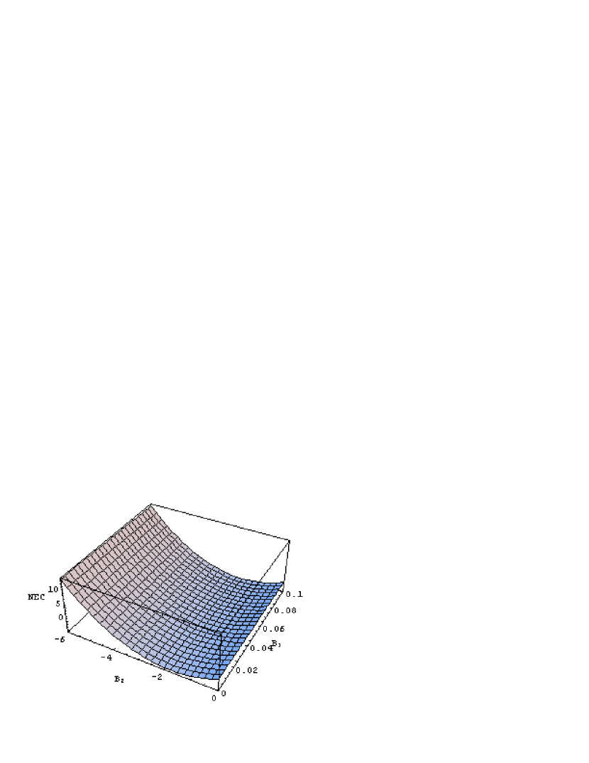
Refer to caption
Refer to caption
Figure 1: The graph at the left side of this figure corresponds to the NEC by plotting 2nρn1(ΛB2B1)+(ρn+B2)22𝑛superscript𝜌𝑛1Λsubscript𝐵2subscript𝐵1superscriptsuperscript𝜌𝑛subscript𝐵222n\rho^{n-1}(\Lambda B_{2}-B_{1})+(\rho^{n}+B_{2})^{2} in functions of B1subscript𝐵1B_{1} and B2subscript𝐵2B_{2} with ρ=0.1𝜌0.1\rho=0.1, n=1𝑛1n=1, Λ=1.7Λ1.7\Lambda=1.7. This case is different from the evident conditions. Here, 2nρn1(ΛB2B1)2𝑛superscript𝜌𝑛1Λsubscript𝐵2subscript𝐵12n\rho^{n-1}(\Lambda B_{2}-B_{1}), but the NEC is realized. The graph at the right side of the figure corresponds to the NEC but in this case by plotting 2nρn1(A1A2Λ)+(A2ρn+1)22𝑛superscript𝜌𝑛1subscript𝐴1subscript𝐴2Λsuperscriptsubscript𝐴2superscript𝜌𝑛122n\rho^{n-1}(A_{1}-A_{2}\Lambda)+(A_{2}\rho^{n}+1)^{2} in functions of A1subscript𝐴1A_{1} and A2subscript𝐴2A_{2} with n=1𝑛1n=-1, Λ=1.7Λ1.7\Lambda=1.7 an ρ=0.1𝜌0.1\rho=0.1. This situation is also different from those of the evident conditions, but also realizes the NEC.
Refer to caption
Refer to caption
Figure 2: The graph at the left side is obtained by plotting the function Λρ2n+2ρ2n+1+4B2ρn+1+2B22ρ+[(1+4n)ΛB2+(14n)B1]ρn+B1B2Λsuperscript𝜌2𝑛2superscript𝜌2𝑛14subscript𝐵2superscript𝜌𝑛12subscriptsuperscript𝐵22𝜌delimited-[]14𝑛Λsubscript𝐵214𝑛subscript𝐵1superscript𝜌𝑛subscript𝐵1subscript𝐵2\Lambda\rho^{2n}+2\rho^{2n+1}+4B_{2}\rho^{n+1}+2B^{2}_{2}\rho+\left[(1+4n)\Lambda B_{2}+(1-4n)B_{1}\right]\rho^{n}+B_{1}B_{2} in terms of suitable values of B1subscript𝐵1B_{1} and B2subscript𝐵2B_{2}, with n=1𝑛1n=1, Λ=1.7Λ1.7\Lambda=1.7 and ρ=0.1𝜌0.1\rho=0.1. We have a situation different from the evident ones but the WEC is satisfied. At the right side of the figure one has the graph obtained by plotting A1A2ρ2n+2ρ2n+1+4A2ρn+1+2ρ+[(1+4n)A1+(14n)A2Λ]ρn+Λsubscript𝐴1subscript𝐴2superscript𝜌2𝑛2superscript𝜌2𝑛14subscript𝐴2superscript𝜌𝑛12𝜌delimited-[]14𝑛subscript𝐴114𝑛subscript𝐴2Λsuperscript𝜌𝑛ΛA_{1}A_{2}\rho^{2n}+2\rho^{2n+1}+4A_{2}\rho^{n+1}+2\rho+\left[(1+4n)A_{1}+(1-4n)A_{2}\Lambda\right]\rho^{n}+\Lambda in terms of A1subscript𝐴1A_{1} and A2subscript𝐴2A_{2}, with n=1𝑛1n=-1, Λ=1.7Λ1.7\Lambda=1.7 and ρ=0.1𝜌0.1\rho=0.1. We also have here a case different from the evident ones but for which the WEC is still realized.
Refer to caption
Refer to caption
Figure 3: At the left side the SEC is represented by plotting 2ρ2n+12Λρ2n+4B2ρn+1+2B22ρ2[(12n)ΛB2+(1+2n)B1]ρn2B1B22superscript𝜌2𝑛12Λsuperscript𝜌2𝑛4subscript𝐵2superscript𝜌𝑛12subscriptsuperscript𝐵22𝜌2delimited-[]12𝑛Λsubscript𝐵212𝑛subscript𝐵1superscript𝜌𝑛2subscript𝐵1subscript𝐵22\rho^{2n+1}-2\Lambda\rho^{2n}+4B_{2}\rho^{n+1}+2B^{2}_{2}\rho-2\left[(1-2n)\Lambda B_{2}+(1+2n)B_{1}\right]\rho^{n}-2B_{1}B_{2} in functions of B1subscript𝐵1B_{1} and B2subscript𝐵2B_{2}, setting Λ=1.7Λ1.7\Lambda=1.7, ρ=0.1𝜌0.1\rho=0.1 and n=1𝑛1n=1. The graph at right side of the figure represents the SEC where 2A22ρ2n+12A1A2ρ2n+4A2ρn+1+2ρ2[(12n)A1+(1+2n)A2Λ]ρn2Λ2superscriptsubscript𝐴22superscript𝜌2𝑛12subscript𝐴1subscript𝐴2superscript𝜌2𝑛4subscript𝐴2superscript𝜌𝑛12𝜌2delimited-[]12𝑛subscript𝐴112𝑛subscript𝐴2Λsuperscript𝜌𝑛2Λ2A_{2}^{2}\rho^{2n+1}-2A_{1}A_{2}\rho^{2n}+4A_{2}\rho^{n+1}+2\rho-2\left[(1-2n)A_{1}+(1+2n)A_{2}\Lambda\right]\rho^{n}-2\Lambda is plotted in terms of A1subscript𝐴1A_{1} and A2subscript𝐴2A_{2}, setting n=1𝑛1n=-1, ρ=0.1𝜌0.1\rho=0.1 and Λ=1.7Λ1.7\Lambda=1.7.
Refer to caption
Refer to caption
Figure 4: The graph at the left side of this figure characterizes the DEC, coming from ρ2n+1+Λρ2n+2B2ρn+1+B22ρ+B1B2+[(2n+1)ΛB2+(12n)B1]ρnsuperscript𝜌2𝑛1Λsuperscript𝜌2𝑛2subscript𝐵2superscript𝜌𝑛1superscriptsubscript𝐵22𝜌subscript𝐵1subscript𝐵2delimited-[]2𝑛1Λsubscript𝐵212𝑛subscript𝐵1superscript𝜌𝑛\rho^{2n+1}+\Lambda\rho^{2n}+2B_{2}\rho^{n+1}+B_{2}^{2}\rho+B_{1}B_{2}+\left[(2n+1)\Lambda B_{2}+(1-2n)B_{1}\right]\rho^{n} plotted in functions of B1subscript𝐵1B_{1} and B2subscript𝐵2B_{2}, by setting n=1𝑛1n=1, ρ=0.1𝜌0.1\rho=0.1 and Λ=1.7Λ1.7\Lambda=1.7, while the graph at the right side represent the DEC from the plot of A22ρ2n+1+A1A2ρ2n+2A2ρn+1+ρ+Λ+[(2n+1)A1+(12n)ΛA2]ρnsubscriptsuperscript𝐴22superscript𝜌2𝑛1subscript𝐴1subscript𝐴2superscript𝜌2𝑛2subscript𝐴2superscript𝜌𝑛1𝜌Λdelimited-[]2𝑛1subscript𝐴112𝑛Λsubscript𝐴2superscript𝜌𝑛A^{2}_{2}\rho^{2n+1}+A_{1}A_{2}\rho^{2n}+2A_{2}\rho^{n+1}+\rho+\Lambda+\left[(2n+1)A_{1}+(1-2n)\Lambda A_{2}\right]\rho^{n} in functions of A1subscript𝐴1A_{1} and A2subscript𝐴2A_{2}, with n=1𝑛1n=-1, ρ=0.1𝜌0.1\rho=0.1 and Λ=1.7Λ1.7\Lambda=1.7.
Refer to caption
Refer to caption
Figure 5: The graph at the left side of this figure represents the NEC and is obtained by plotting ρ+2qma3+ρlnq1(b3ρm)𝜌2𝑞𝑚subscript𝑎3𝜌superscript𝑞1subscript𝑏3superscript𝜌𝑚\rho+2qma_{3}+\rho\ln^{q-1}{\left(b_{3}\rho^{m}\right)} in functions of m𝑚m and b3subscript𝑏3b_{3}, setting ρ=0.1𝜌0.1\rho=0.1, a3=1subscript𝑎31a_{3}=1 and q=3𝑞3q=3. This case is different from the evident conditions but still realizes the NEC. The graph at the right side of the figure corresponds to the WEC, plotting 2ρ+2qma3+(ρ+2qma3)lnq1(b3ρm)+a3lnq(b3ρm)2𝜌2𝑞𝑚subscript𝑎3𝜌2𝑞𝑚subscript𝑎3superscript𝑞1subscript𝑏3superscript𝜌𝑚subscript𝑎3superscript𝑞subscript𝑏3superscript𝜌𝑚2\rho+2qma_{3}+\left(\rho+2qma_{3}\right)\ln^{q-1}{\left(b_{3}\rho^{m}\right)}+a_{3}\ln^{q}{\left(b_{3}\rho^{m}\right)} in functions of m𝑚m and b3subscript𝑏3b_{3}, where we set q=3𝑞3q=3, a3=1subscript𝑎31a_{3}=1 and ρ=0.1𝜌0.1\rho=0.1.
Refer to caption
Refer to caption
Figure 6: The graph at the left side characterizes the SEC is obtained by plotting 2ρ+2qma3+(ρ+2qma3)lnq1(b3ρm)2a3lnq(b3ρm)2𝜌2𝑞𝑚subscript𝑎3𝜌2𝑞𝑚subscript𝑎3superscript𝑞1subscript𝑏3superscript𝜌𝑚2subscript𝑎3superscript𝑞subscript𝑏3superscript𝜌𝑚2\rho+2qma_{3}+\left(\rho+2qma_{3}\right)\ln^{q-1}{\left(b_{3}\rho^{m}\right)}-2a_{3}\ln^{q}{\left(b_{3}\rho^{m}\right)} in functions of m𝑚m and b3subscript𝑏3b_{3} where we set ρ=0.1𝜌0.1\rho=0.1, a3=103subscript𝑎3superscript103a_{3}=10^{-3} and q=3𝑞3q=3. This situation is different from the evident conditions, but also realizes the SEC. The graph at the right side of the figure is obtained by plotting 3ρ+2qma3+(ρ+4qma3)lnq1(b3ρm)+3a3lnq(b3ρm)3𝜌2𝑞𝑚subscript𝑎3𝜌4𝑞𝑚subscript𝑎3superscript𝑞1subscript𝑏3superscript𝜌𝑚3subscript𝑎3superscript𝑞subscript𝑏3superscript𝜌𝑚3\rho+2qma_{3}+\left(\rho+4qma_{3}\right)\ln^{q-1}{\left(b_{3}\rho^{m}\right)}+3a_{3}\ln^{q}{\left(b_{3}\rho^{m}\right)} in functions of m𝑚m and b3subscript𝑏3b_{3}, with q=3𝑞3q=3, a3=1subscript𝑎31a_{3}=1 and ρ=0.1𝜌0.1\rho=0.1. This graph represents the DEC.